Birkhoff Normal Forms, KAM Theory and Time Reversal Symmetry for Certain Rational Map

Abstract

By using the KAM(Kolmogorov-Arnold-Moser) theory and time reversal symmetries, we investigate the stability of the equilibrium solutions of the system:

$$x_{n+1}=\frac{1}{y_n},y_{n+1}=\frac{\beta x_n}{1+y_n},n=0,1,2,\dots ,$$

where the parameter $\beta >0,$ and initial conditions $x_0$ and $y_0$ are positive numbers. We obtain the Birkhoff normal form for this system and prove the existence of periodic points with arbitrarily large periods in every neighborhood of the unique positive equilibrium. We use invariants to find a Lyapunov function and Morse’s lemma to prove closedness of invariants. We also use the time reversal symmetry method to effectively find some feasible periods and the corresponding periodic orbits.

1. Introduction

The following rational system of difference equations:

$$\left\{\begin{array}{ccc}\hfill x_{n+1}& =& \frac{1}{y_n}\hfill \\ \hfill y_{n+1}& =& \frac{\beta x_n}{1+y_n}\hfill \end{array}\right.,n=0,1,\dots$$

(1)

and the corresponding equation:

$$y_{n+1}=\frac{\beta }{y_{n-1}(1+y_n)}n=0,1,\dots ,$$

(2)

where the parameter $\beta >0$ and initial conditions $x_0,y_0$ are positive numbers were considered in [1] and [2]. The authors established the boundedness of all solutions of system (1) by using the invariant:

$$I(x_n,y_n)=\beta x_n+y_n+\frac{1}{x_n}+\frac{\beta }{y_n}+\frac{y_n}{x_n}.$$

(3)

Equation (2) and its invariant (3), where $x_n=1/y_{n-1}$ were obtained in [3,4] and the stability of the equilibrium by means of Lyapunov function generated by invariant (3) was derived in [5,6], (pp. 247–250). Equation (2) is also a special case of equation:

$$y_{n+1}=\frac{B{y}_n{y}_{n-1}+E{y}_{n-1}+F}{b{y}_n{y}_{n-1}+e{y}_{n-1}+f}n=0,1,\dots$$

(4)

with all nonnegative coefficients and initial conditions. Equation (4) is a rational difference equation with quadratic terms which is a subject of recent research, see [7,8,9,10].

In this paper, we will show that the corresponding map can be transformed into an area preserving map for which we will find the Birkhoff Normal form, and, using it, we will apply the KAM theorem to prove the stability of the unique positive equilibrium and the existence of periodic points with an arbitrarily large period in every neighborhood of the unique positive equilibrium. In addition, we prove that the corresponding map is conjugate to its inverse map through the involution map. Then, we will use this conjugacy to find some feasible periods of this map. The KAM theory will be enough to prove the stability of the equilibrium for $\beta \ne 2$, and then we use the invariant (3) and Morse’s lemma to prove the stability in the remaining case $\beta =2$, see [5]. In addition, Morse’s lemma implies that all invariants are locally simple closed curves. A very recent paper [11] gives some effective tests for difference equation to have a continuous invariant. The method of invariants for the construction of a Lyapunov function and proving stability of the equilibrium points was used successfully in [5,6,12], and the KAM theory was used for the same objective in [12,13,14,15,16]. The class of difference equations which admit an invariant is not a large class even in the case of rational difference equations, see [11]. In the case when a difference equation’s corresponding map is area preserving and does not possess an invariant, the only tool left seems to be KAM theory, see [17] for such an example. Furthermore, the corresponding Equation (4) can be embedded by iteration into a fourth order difference equation:

$$y_{n+1}=\frac{y_{n-2}{y}_{n-3}(1+y_{n-1})(1+y_{n-2})}{\beta +y_{n-2}(1+y_{n-1})},n=0,1,\dots ,$$

which is increasing in all its arguments and yet exhibits the chaos.

Let T be the map associated to the system (1), i.e.,

$$T\left(\begin{array}{c}x\\ y\end{array}\right)=\left(\begin{array}{c}\frac{1}{y}\\ \frac{\beta x}{1+y}\end{array}\right).$$

(5)

The map (5) has the unique fixed point $(1/\overline{y},\overline{y})$ in the positive quadrant, where

$${\overline{y}}^2(1+\overline{y})=\beta .$$

An invertible map $T:{\mathbb{R}}^2\to {\mathbb{R}}^2$ is area preserving if the area of $T\left(A\right)$ equals the area of A for all measurable subsets A [6,18,19]. As is known, a differentiable map T is area preserving if the determinant of its Jacobian matrix is equal $\pm 1$, that is $det{J}_T=\pm 1$ at every point of domain of T, see [18,19]. We claim that in logarithmic coordinates $(u,v)$ where $u=ln\left(\overline{y}x\right)$, and $v=ln(y/\overline{y})$, the map (5) is area preserving.

Lemma 1. 

The map (5) is an area preserving map in the logarithmic coordinates.

Proof. 

The Jacobian matrix of the map T is

$$J_T(x,y)=\left(\begin{array}{cc}0& -\frac{1}{y^2}\\ \frac{\beta }{y+1}& -\frac{\beta x}{{(y+1)}^2}\end{array}\right)$$

(6)

with

$$det{J}_T(x,y)=\frac{\beta }{y^2(y+1)}.$$

We substitute $u=ln\left(\overline{y}x\right)$, $v=ln(y/\overline{y})$ and rewrite the map in $(u,v)$ coordinates to obtain the map

$$\left(\begin{array}{c}u\\ v\end{array}\right)\to \left(\begin{array}{c}-v\\ ln\beta +u-ln\left(e^v\overline{y}+1\right)-2ln\overline{y}\end{array}\right).$$

The Jacobian matrix of this map is

$$J_T(u,v)=\left(\begin{array}{cc}0& -1\\ 1& \frac{1}{e^v\overline{y}+1}-1\end{array}\right),$$

(7)

and so $det{J}_T(u,v)=1$. ☐

A fixed point $(\overline{x},\overline{y})$ is an elliptic point of an area preserving map if the eigenvalues of $J_T(\overline{x},\overline{y})$ form a purely imaginary, complex conjugate pair $\lambda ,\overline{\lambda }$, see [6,18].

Lemma 2. 

The map T in $(x,y)$ coordinates has an elliptic fixed point $(1/\overline{y},\overline{y})$. In the logarithmic coordinates, the corresponding fixed point is $(0,0).$

Proof. 

For the fixed points in $(x,y)$ coordinates, solving $1/y=x$ and $\beta x/(1+y)=y$ yields the fixed point $(1/\overline{y},\overline{y})$ where $\overline{y}$ is the unique positive solution of ${\overline{y}}^2(1+\overline{y})=\beta .$ Evaluating the Jacobian matrix (6) of T at $(1/\overline{y},\overline{y})$ gives

$$J_T(1/\overline{y},\overline{y})=\left(\begin{array}{cc}0& -\frac{1}{{\overline{y}}^2}\\ \frac{\beta }{\overline{y}+1}& -\frac{\beta }{\overline{y}{\left(\overline{y}+1\right)}^2}\end{array}\right).$$

By using $\beta ={\overline{y}}^3+{\overline{y}}^2$, we obtain that the eigenvalues of $J_T(1/\overline{y},\overline{y})$ are $\lambda ,\overline{\lambda }$ where

$$\lambda =\frac{-\overline{y}+i\sqrt{\left(\overline{y}+2\right)\left(3\overline{y}+2\right)}}{2\left(\overline{y}+1\right)}.$$

(8)

Since $\left|\lambda \right|=1$, we have that $(1/\overline{y},\overline{y})$ is an elliptic fixed point.

Under the logarithmic coordinate change $(x,y)\to (u,v)$, the fixed point $(1/\overline{y},\overline{y})$ becomes $(0,0)$. Evaluating the Jacobian matrix (7) of T at $(0,0)$ gives

$$J_T(0,0)=\left(\begin{array}{cc}0& -1\\ 1& \frac{1}{\overline{y}+1}-1\end{array}\right)$$

with eigenvalues which are given by Equation (8). ☐

The rest of the paper is organized into three sections. The second section contains a derivation of the Birkhoff normal form for map T and an application of the KAM theory, which proves stability of the equilibrium and the existence of an infinite number of periodic solutions for $\beta \ne 2$. The third section makes use of the invariant (3) in proving stability for $\beta =2$ and the construction of a Lyapunov function. The fourth section uses the symmetries for the map T showing that this map is conjugate to its inverse through an involution. Then, we use time reversal symmetry method [13,20] based on the symmetries to effectively find some feasible periods and corresponding orbits of the map T.

2. The KAM Theory and Birkhoff Normal Form

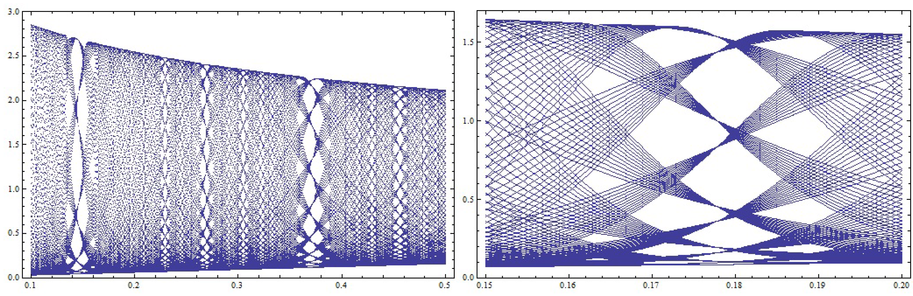
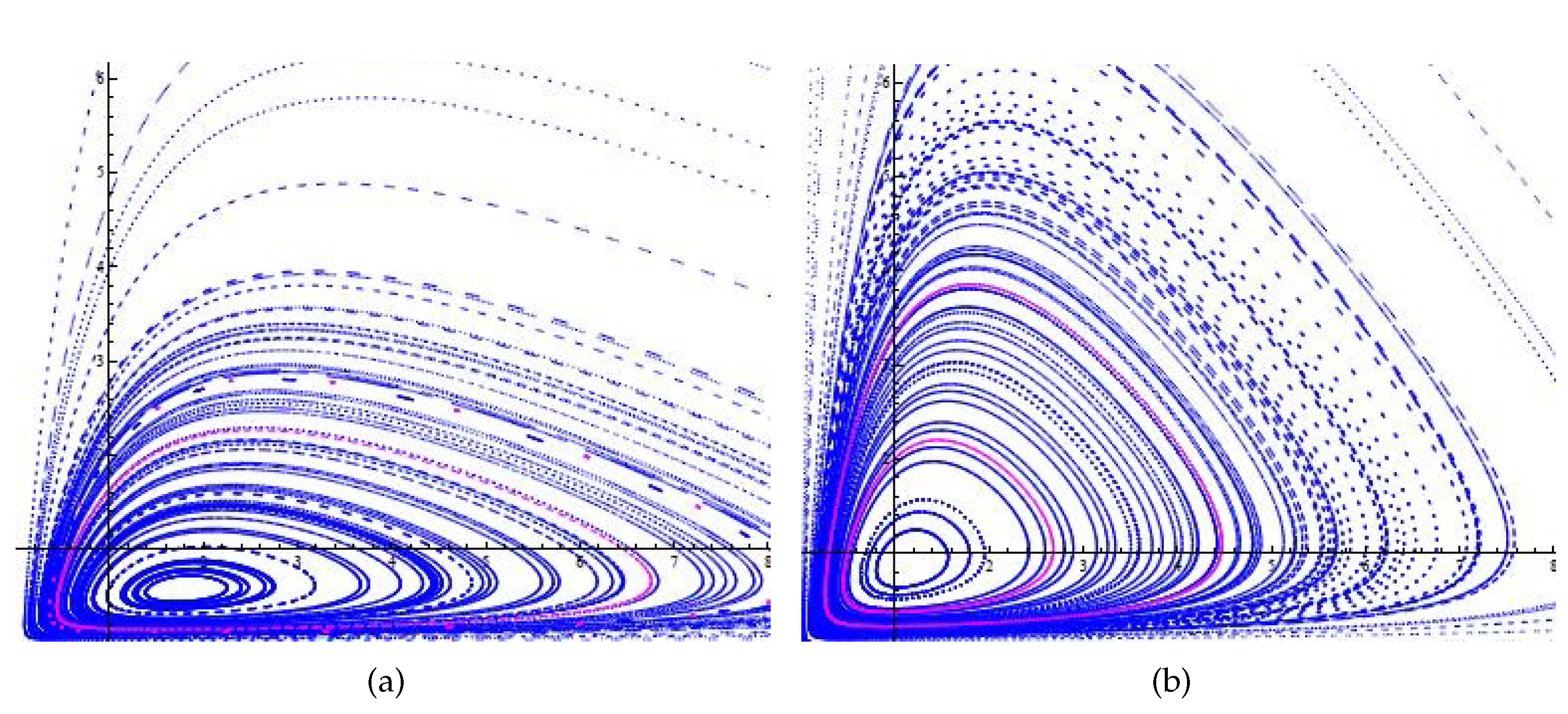
The KAM Theorem asserts that, in any sufficiently small neighborhood of a non degenerate elliptic fixed point of a smooth area-preserving map, there exists many invariant closed curves. We explain this theorem in some detail. Consider a smooth, area-preserving map $(x,y)\to T(x,y)$ of the plane that has $(0,0)$ as an elliptic fixed point. After a linear transformation, one can represent the map in the form

$$z\to \lambda z+g(z,\overline{z}),$$

where λ is the eigenvalue of the elliptic fixed point, $z=x+iy$ and $\overline{z}=x-iy$ are complex variables, and g vanishes with its derivative at $z=0$. Assume that the eigenvalue λ of the elliptic fixed point satisfies the non-resonance condition ${\lambda }^k\ne 1$ for $k=1,\dots ,q$, for some $q\ge 4$. Then, Birkhoff showed that there exists new, canonical complex coordinates $(\zeta ,\overline{\zeta })$ relative to which the mapping takes the normal form

$$\zeta \to \lambda \zeta e^{i\tau \left(\zeta \overline{\zeta }\right)}+h(\zeta ,\overline{\zeta })$$

in a neighborhood of the elliptic fixed point, where $\tau \left(\zeta \overline{\zeta }\right)={\tau }_1{\left|\zeta \right|}^2+\dots +{\tau }_s{\left|\zeta \right|}^{2s}$ is a real polynomial, $s=\left[\right(q-2)/2]$ and h vanishes with its derivatives up to order $q-1$. The numbers ${\tau }_1,\dots ,{\tau }_s$ are called twist coefficients. Consider an invariant annulus $ϵ<\left|\zeta \right|<2ϵ$ in a neighborhood of an elliptic fixed point, for ϵ, a very small positive number. Note that, if we neglect the remainder h, the normal form approximation $\zeta \to \lambda \zeta e^{i\tau (\zeta \overline{\zeta })}$ leaves invariant all circles ${\left|\zeta \right|}^2=const$. The motion restricted to each of these circles is a rotation by some angle. In addition, please note that, if at least one of the twist coefficients ${\tau }_j$ is nonzero, the angle of rotation will vary from circle to circle. A radial line through the fixed point will undergo twisting under the map. The KAM theorem (Moser’s twist theorem) says that, under the addition of the remainder term, most of these invariant circles will survive as invariant closed curves under the full map.

Theorem 3. 

Assume that $\tau \left(\zeta \overline{\zeta }\right)$ is not identically zero and ϵ is sufficiently small, then the map T has a set of invariant closed curves of positive Lebesque measure close to the original invariant circles. Moreover, the relative measure of the set of surviving invariant curves approaches full measure as ϵ approaches 0. The surviving invariant closed curves are filled with dense irrational orbits.

The KAM theorem requires that the elliptic fixed point be non-resonant and non degenerate. Note that for $q=4$ the non-resonance condition ${\lambda }^k\ne 1$ requires that $\lambda \ne \pm 1$ or $\pm i$. The above normal form yields the approximation

$$\zeta \to \lambda \zeta +c_1{\zeta }^2\overline{\zeta }+{O\left(\right|\zeta |}^4)$$

with $c_1=i\lambda {\tau }_1$ and ${\tau }_1$ being the first twist coefficient. We will call an elliptic fixed point non-degenerate if ${\tau }_1\ne 0$.

Consider a general map T that has a fixed point at the origin with complex eigenvalues λ and $\overline{\lambda }$ satisfying $\left|\lambda \right|=1$ and $Im\left(\lambda \right)\ne 0.$ By putting the linear part of such a map into Jordan Normal form, we may assume that T has the following form near the origin

$$T\left(\begin{array}{c}{x}_1\\ x_2\end{array}\right)=\left(\begin{array}{cc}Re\left(\lambda \right)& -Im\left(\lambda \right)\\ Im\left(\lambda \right)& Re\left(\lambda \right)\end{array}\right)\left(\begin{array}{c}{x}_1\\ x_2\end{array}\right)+\left(\begin{array}{c}{g}_1(x_1,x_2)\\ g_2(x_1,x_2)\end{array}\right).$$

One can now pass to the complex coordinates $z=x_1+i{x}_2$ to obtain the complex form of the system

$$z\to \lambda z+{\xi }_{20}{z}^2+{\xi }_{11}z\overline{z}+{\xi }_{02}{\overline{z}}^2+{\xi }_{30}{z}^3+{\xi }_{21}{z}^2\overline{z}+{\xi }_{12}z{\overline{z}}^2+{\xi }_{03}{\overline{z}}^3+{O\left(\right|z|}^4).$$

The coefficient $c_1$ can be computed directly using the formula below derived by Wan in the context of Hopf bifurcation theory [21]. In [22], it is shown that, when one uses area-preserving coordinate changes, Wan’s formula yields the twist coefficient ${\tau }_1$ that is used to verify the non-degeneracy condition necessary to apply the KAM theorem. We use the formula:

$$c_1=\frac{{\xi }_{20}{\xi }_{11}(\overline{\lambda }+2\lambda -3)}{({\lambda }^2-\lambda )(\overline{\lambda }-1)}+\frac{|{\xi }_{11}{|}^2}{1-\overline{\lambda }}+\frac{2|{\xi }_{02}{|}^2}{{\lambda }^2-\overline{\lambda }}+{\xi }_{21},$$

where

$${\xi }_{20}=\frac{1}{8}\left\{{\left(g_1\right)}_{x_1{x}_1}-{\left(g_1\right)}_{x_2{x}_2}+2{\left(g_2\right)}_{x_1{x}_2}+i\left[{\left(g_2\right)}_{x_1{x}_1}-{\left(g_2\right)}_{x_2{x}_2}-2{\left(g_1\right)}_{x_1{x}_2}\right]\right\},$$

$${\xi }_{11}=\frac{1}{4}\left\{{\left(g_1\right)}_{x_1{x}_1}+{\left(g_1\right)}_{x_2{x}_2}+i\left[{\left(g_2\right)}_{x_1{x}_1}+{\left(g_2\right)}_{x_2{x}_2}\right]\right\},$$

$${\xi }_{02}=\frac{1}{8}\left\{{\left(g_1\right)}_{x_1{x}_1}-{\left(g_1\right)}_{x_2{x}_2}-2{\left(g_2\right)}_{x_1{x}_2}+i\left[{\left(g_2\right)}_{x_1{x}_1}-{\left(g_2\right)}_{x_2{x}_2}+2{\left(g_1\right)}_{x_1{x}_2}\right]\right\},$$

$${\xi }_{21}=\frac{1}{16}\left({\left(g_1\right)}_{x_1{x}_1{x}_1}+{\left(g_1\right)}_{x_1{x}_2{x}_2}+{\left(g_2\right)}_{x_1{x}_1{x}_2}+{\left(g_2\right)}_{x_2{x}_2{x}_2}\right),$$

$$+\frac{i}{16}\left({\left(g_2\right)}_{x_1{x}_1{x}_1}+{\left(g_2\right)}_{x_1{x}_2{x}_2}-{\left(g_1\right)}_{x_1{x}_1{x}_2}-{\left(g_1\right)}_{x_2{x}_2{x}_2}\right).$$

Theorem 4. 

The elliptic fixed point $(0,0)$, in the $(u,v)$ coordinates, is non-degenerate for $\beta \ne 2$ and non-resonant for $\beta >0.$

Proof. 

Let F be the function defined by

$$F\left(\begin{array}{c}u\\ v\end{array}\right)=\left(\begin{array}{c}-v\\ ln\beta +u-ln\left(e^v\overline{y}+1\right)-2ln\overline{y}\end{array}\right).$$

Then, F has the unique elliptic fixed point $(0,0).$ The Jacobian matrix of F at $(u,v)$ is given by

$$J_F(u,v)=\left(\begin{array}{cc}0& -1\\ 1& \frac{1}{e^v\overline{y}+1}-1\end{array}\right).$$

At $(0,0),$$J_F(u,v)$ has the form

$$J_0=J_F(0,0)=\left(\begin{array}{cc}0& -1\\ 1& \frac{1}{\overline{y}+1}-1\end{array}\right).$$

(9)

The eigenvalues of (9) are λ and $\overline{\lambda }$ where

$$\lambda =\frac{-\overline{y}+i\sqrt{\left(\overline{y}+2\right)\left(3\overline{y}+2\right)}}{2\left(\overline{y}+1\right)}.$$

One can prove that

$$\left|\lambda \right|=1$$

$$\begin{array}{cc}\hfill {\lambda }^2=& -\frac{\overline{y}\left(\overline{y}+4\right)+2}{2{\left(\overline{y}+1\right)}^2}-\frac{i\sqrt{\left(\overline{y}+2\right)\left(3\overline{y}+2\right)}\overline{y}}{\left(\overline{y}+1\right)\left(2\overline{y}+2\right)}\hfill \\ \hfill {\lambda }^3=& \frac{\overline{y}\left(2\overline{y}\left(\overline{y}+3\right)+3\right)}{2{\left(\overline{y}+1\right)}^3}-\frac{i\left(2\overline{y}+1\right)\sqrt{\left(\overline{y}+2\right)\left(3\overline{y}+2\right)}}{2{\left(\overline{y}+1\right)}^3}\hfill \\ \hfill {\lambda }^4=& \frac{\overline{y}\left(-{\overline{y}}^3+8\overline{y}+8\right)+2}{2{\left(\overline{y}+1\right)}^4}+\frac{i\overline{y}\sqrt{\left(\overline{y}+2\right)\left(3\overline{y}+2\right)}\left(\overline{y}\left(\overline{y}+4\right)+2\right)}{2{\left(\overline{y}+1\right)}^4}\hfill \end{array},$$

from which follows that ${\lambda }^k\ne 1$ for $k=1,2,3,4$ and $\beta >0.$

Now, we have that

$$F\left(\begin{array}{c}u\\ v\end{array}\right)=\left(\begin{array}{cc}0& -1\\ 1& \frac{1}{\overline{y}+1}-1\end{array}\right)\left(\begin{array}{c}u\\ v\end{array}\right)+\left(\begin{array}{c}{f}_1(\delta ,u,v)\\ f_2(\delta ,u,v)\end{array}\right),$$

where

$$\begin{array}{cc}\hfill f_1(\delta ,u,v)=& 0,\hfill \\ \hfill f_2(\delta ,u,v)=& \frac{v\overline{y}}{\overline{y}+1}-ln\left(e^v\overline{y}+1\right)-2ln\overline{y}+ln\beta \hfill \end{array}.$$

Then, the system $(u_{n+1},v_{n+1})=F(u_n,v_n)$ is equivalent to

$$\left(\begin{array}{c}{u}_{n+1}\\ v_{n+1}\end{array}\right)=\left(\begin{array}{cc}0& -1\\ 1& \frac{1}{\overline{y}+1}-1\end{array}\right)\left(\begin{array}{c}{u}_n\\ v_n\end{array}\right)+\left(\begin{array}{c}{f}_1(u_n,v_n)\\ f_2(u_n,v_n)\end{array}\right).$$

Let

$$\left(\begin{array}{c}{u}_n\\ v_n\end{array}\right)=P\left(\begin{array}{c}{\tilde{u}}_n\\ {\tilde{v}}_n\end{array}\right),$$

where

$$P=\frac{1}{\sqrt{D}}\left(\begin{array}{cc}\frac{\overline{y}}{2\left(\overline{y}+1\right)}& -\frac{\sqrt{\left(\overline{y}+2\right)\left(3\overline{y}+2\right)}}{2\left(\overline{y}+1\right)}\\ 1& 0\end{array}\right),P^{-1}=\sqrt{D}\left(\begin{array}{cc}0& 1\\ -\frac{2\left(\overline{y}+1\right)}{\sqrt{\left(\overline{y}+2\right)\left(3\overline{y}+2\right)}}& \frac{\overline{y}}{\sqrt{\left(\overline{y}+2\right)\left(3\overline{y}+2\right)}}\end{array}\right)$$

and

$$D=\frac{\sqrt{\left(\overline{y}+2\right)\left(3\overline{y}+2\right)}}{2\left(\overline{y}+1\right)}.$$

Thus, the system $(u_{n+1},v_{n+1})=F(u_n,v_n)$ is transformed into its Birkhoff normal form

$$\left(\begin{array}{c}{\tilde{u}}_{n+1}\\ {\tilde{v}}_{n+1}\end{array}\right)=\left(\begin{array}{cc}-\frac{\overline{y}}{2\overline{y}+2}& -\frac{\sqrt{\left(\overline{y}+2\right)\left(3\overline{y}+2\right)}}{2\left(\overline{y}+1\right)}\\ \frac{\sqrt{\left(\overline{y}+2\right)\left(3\overline{y}+2\right)}}{2\overline{y}+2}& -\frac{\overline{y}}{2\overline{y}+2}\end{array}\right)\left(\begin{array}{c}{\tilde{u}}_n\\ {\tilde{v}}_n\end{array}\right)+P^{-1}H\left(P\left(\begin{array}{c}{\tilde{u}}_n\\ {\tilde{v}}_n\end{array}\right)\right),$$

where

$$H\left(\begin{array}{c}u\\ v\end{array}\right):=\left(\begin{array}{c}{f}_1(u,v)\\ f_2(u,v)\end{array}\right).$$

Let

$$G\left(\begin{array}{c}u\\ v\end{array}\right)=\left(\begin{array}{c}{g}_1(u,v)\\ g_2(u,v)\end{array}\right)=P^{-1}H\left(P\left(\begin{array}{c}u\\ v\end{array}\right)\right).$$

By a straightforward calculation, we obtain that

$$\begin{array}{cc}\hfill g_1(u,v)=& \sqrt{D}\left(\frac{u\overline{y}}{\sqrt{D}\left(\overline{y}+1\right)}-ln\left(\overline{y}{e}^{\frac{u}{\sqrt{D}}}+1\right)-2ln\overline{y}+ln\beta \right)\hfill \\ \hfill g_2(u,v)=& \frac{\overline{y}\left(\sqrt{D}\left(\overline{y}+1\right)\left(-ln\left(\overline{y}{e}^{\frac{u}{\sqrt{D}}}+1\right)-2ln\overline{y}+ln\beta \right)+u\overline{y}\right)}{\left(\overline{y}+1\right)\sqrt{\left(\overline{y}+2\right)\left(3\overline{y}+2\right)}}\hfill \end{array}.$$

Another calculation gives

$$\begin{array}{cc}\hfill {\xi }_{20}{|}_{u=v=0}=& -\frac{\overline{y}\left(\sqrt{\left(\overline{y}+2\right)\left(3\overline{y}+2\right)}+i\overline{y}\right)}{8\sqrt{D}{\left(\overline{y}+1\right)}^2\sqrt{\left(\overline{y}+2\right)\left(3\overline{y}+2\right)}}\hfill \\ \hfill {\xi }_{11}{|}_{u=v=0}=& -\frac{\overline{y}\left(1+\frac{i\overline{y}}{\sqrt{\left(\overline{y}+2\right)\left(3\overline{y}+2\right)}}\right)}{4\sqrt{D}{\left(\overline{y}+1\right)}^2}\hfill \\ \hfill {\xi }_{02}{|}_{u=v=0}=& -\frac{\overline{y}\left(\sqrt{\left(\overline{y}+2\right)\left(3\overline{y}+2\right)}+i\overline{y}\right)}{8\sqrt{D}{\left(\overline{y}+1\right)}^2\sqrt{\left(\overline{y}+2\right)\left(3\overline{y}+2\right)}}\hfill \\ \hfill {\xi }_{21}{|}_{u=v=0}=& \frac{\left(\overline{y}-1\right)\overline{y}\left(\sqrt{\left(\overline{y}+2\right)\left(3\overline{y}+2\right)}+i\overline{y}\right)}{16D{\left(\overline{y}+1\right)}^3\sqrt{\left(\overline{y}+2\right)\left(3\overline{y}+2\right)}}\hfill \end{array}.$$

By using

$$\begin{array}{cc}\hfill {\xi }_{20}{\xi }_{11}=& \frac{{\overline{y}}^2{\left(\sqrt{\left(\overline{y}+2\right)\left(3\overline{y}+2\right)}+i\overline{y}\right)}^2}{32D{\left(\overline{y}+1\right)}^4\left(\overline{y}+2\right)\left(3\overline{y}+2\right)}\hfill \\ \hfill {\xi }_{11}\overline{{\xi }_{11}}=& \frac{{\overline{y}}^2}{4D{\left(\overline{y}+1\right)}^2\left(3{\overline{y}}^2+8\overline{y}+4\right)}\hfill \\ \hfill {\xi }_{02}\overline{{\xi }_{02}}=& \frac{{\overline{y}}^2}{16D{\left(\overline{y}+1\right)}^2\left(3{\overline{y}}^2+8\overline{y}+4\right)}\hfill \end{array},$$

a straightforward calculation yields

$$\begin{array}{cc}\hfill c_1& =\frac{{\xi }_{20}{\xi }_{11}(\overline{\lambda }+2\lambda -3)}{({\lambda }^2-\lambda )(\overline{\lambda }-1)}+\frac{|{\xi }_{11}{|}^2}{1-\overline{\lambda }}+\frac{2|{\xi }_{02}{|}^2}{{\lambda }^2-\overline{\lambda }}+{\xi }_{21}\hfill \\ & =\frac{\left(\overline{y}-1\right)\overline{y}\left(\overline{y}+1\right)}{\left(3\overline{y}+2\right)\sqrt{\left(\overline{y}+2\right)\left(3\overline{y}+2\right)}\left(4+\overline{y}\left(3\overline{y}-i\sqrt{\left(\overline{y}+2\right)\left(3\overline{y}+2\right)}+8\right)\right)}\hfill \end{array}.$$

It can be proved that

$${\tau }_1=-i\overline{\lambda }{c}_1=-\frac{\left(\overline{y}-1\right)\overline{y}}{2\left(\overline{y}+2\right){\left(3\overline{y}+2\right)}^2},$$

which implies that ${\tau }_1\ne 0$ for $\beta \ne 2$ since ${\overline{y}}^2(1+\overline{y})=\beta .$ ☐

 ☐

The following result is a consequence of Moser’s twist map theorem [13,19,23,24].

Theorem 5. 

Let T be a map (5) associated to the system (1), and $(\overline{x},\overline{y})$ be a non-degenerate elliptic fixed point. If $\beta \ne 2$, then there exist periodic points with arbitrarily large periods in every neighborhood of $(\overline{x},\overline{y}).$ In addition, $(\overline{x},\overline{y})$ is a stable fixed point.

3. Invariant

In this section, we use the invariant to find a Lyapunov function and prove stability of the equilibrium for all values of parameter $\beta >0$, see [5,6] for similar results.

Lemma 6. 

The unique equilibrium $(\frac{1}{\overline{y}},\overline{y})$ of Equation (1) is a critical point of the invariant (3).

Proof. 

The system (1) possesses an invariant given by Equation (3). The function $I(x,y)$ associated with Equation (3) has partial derivatives

$$\frac{\partial I}{\partial x}=\beta -\frac{1}{x^2}-\frac{y}{x^2},\frac{\partial I}{\partial y}=1-\frac{\beta }{y^2}+\frac{1}{x}.$$

(10)

The unique equilibrium of Equation (1) satisfies that $\overline{x}=\frac{1}{\overline{y}}$ and ${\overline{y}}^2(1+\overline{y})=\beta$. Hence $\overline{x}$ is the unique positive solution of the equation $\beta x^3-x-1=0$. Equation (10) implies that any critical point $(x,y)$ of Equation (3) satisfies $y=\beta x^2-1$ and $(x+1)y^2-\beta x=0$. Substitution yields

$${\beta }^2{x}^5+{\beta }^2{x}^4-2\beta x^3-2\beta x^2+(1-\beta )x+1=0.$$

(11)

Equation (11) can be rewritten as

$$(\beta x^3-x-1)(\beta x^2+\beta x-1)=0,$$

which has $\overline{x}$ as a solution. Ⅰ

Lemma 7. 

The graph of the function $I(x,y)$ associated with Equation (3) is a simple closed curve in a neighborhood of the equilibrium of Equation (1). The equilibrium point $(\overline{x},\overline{y})$ is stable.

Proof. 

The Hessian matrix associated with $I(x,y)$ is

$$H(x,y)=\left[\begin{array}{cc}{\displaystyle \frac{2}{x^3}}+{\displaystyle \frac{2y}{x^3}}& -{\displaystyle \frac{1}{x^2}}\\ -{\displaystyle \frac{1}{x^2}}& {\displaystyle \frac{2\beta }{y^3}}\end{array}\right]$$

with determinant

$$det\left(H(x,y)\right)={\displaystyle \frac{4\beta (1+y)}{x^3{y}^3}}-{\displaystyle \frac{1}{x^4}}.$$

For $(x,y)$ a critical point of $I(x,y)$,

$$det\left(H(x,y)\right)=\frac{4{\beta }^2}{x{y}^3}-\frac{1}{x^4}.$$

(12)

For $(\overline{x},\overline{y})$ the unique equilibrium of Equation (1), we can further reduce Equation (12) to

$$det\left(H(\overline{x},\overline{y})\right)=\frac{4{\beta }^2\overline{y}}{{\overline{y}}^3}-{\overline{y}}^4=\frac{4{\beta }^2-{\overline{y}}^6}{{\overline{y}}^2}.$$

Note that since the equation $\beta x^3-x-1=0$ has $\overline{x}$ as its unique positive solution, the equation $\beta /y^3-1/y-1=\frac{\beta -y^2-y^3}{y^3}=0$ has $\overline{y}$ as its unique positive solution. Let us define $f\left(y\right)=y^3+y^2-\beta$. We observe that $f\left(0\right)=-\beta <0$ and $f\left(\sqrt[6]{4{\beta }^2}\right)=2\beta +\sqrt[3]{4{\beta }^2}-\beta >0$, which guarantees that $0<\overline{y}<\sqrt[6]{4{\beta }^2}$. Now the Morse’s lemma [18] guarantees the result provided $det\left(H(\overline{x},\overline{y})\right)>0$. However, $\frac{4{\beta }^2-{\overline{y}}^6}{{\overline{y}}^2}>0$ if and only if $\overline{y}<\sqrt[6]{4{\beta }^2}$, which is indeed the case. In view of the Morse’s lemma [18], the level sets of the function $I(x,y)$ are diffeomorphic to circles in the neighborhood of $(\overline{x},\overline{y})$. In addition, the function

$$V(x,y)=I(x,y)-I(\overline{x},\overline{y})$$

is a Lyapunov function, and so the equilibrium point $(\overline{x},\overline{y})$ is stable, see [5]. ☐

See Figure 1 for the family of invariant curves around the equilibrium. See Figure 2 for the bifurcation diagrams which indicate the appearance of chaos.

4. Symmetries

In the study of area-preserving maps, symmetries play an important role since they yield special dynamic behavior. A transformation R of the plane is said to be a time reversal symmetry for T if $R^{-1}\circ T\circ R=T^{-1}$, meaning that applying the transformation R to the map T is equivalent to iterating the map backwards in time, see [13,20]. If the time reversal symmetry R is an involution, i.e., $R^2=id,$ then the time reversal symmetry condition is equivalent to $R\circ T\circ R=T^{-1},$ and T can be written as the composition of two involutions $T=I_1\circ I_0$, with $I_0=R$ and $I_1=T\circ R.$ Note that if $I_0=R$ is a reversor, then so is $I_1=T\circ R.$ In addition, the jth involution, defined as $I_j:=T^j\circ R,$ is also a reversor.

The invariant sets of the involution maps,

$$S_{0,1}=\left\{(x,y)\right|I_{0,1}(x,y)=(x,y)\}$$

are one-dimensional sets called the symmetry lines of the map. Once the sets $S_{0,1}$ are known, the search for periodic orbits can be reduced to a one-dimensional root finding problem using the following result, see [13,20]:

Theorem 8. 

If $(x,y)\in S_{0,1}$ then $T^n(x,y)=(x,y)$ if and only if

$$\left\{\begin{array}{cc}{T}^{n/2}(x,y)\in S_{0,1},\hfill & forneven;\hfill \\ T^{(n\pm 1)/2}(x,y)\in S_{1,0},\hfill & fornodd.\hfill \end{array}\right.$$

That is, according to this result, periodic orbits can be found by searching in the one-dimensional sets $S_{0,1},$ rather than in the whole domain. Periodic orbits of different orders can then be found at the intersection of the symmetry lines $S_j$ $j=1,2,...$ associated to the jth involution; for example, if $(x,y)\in S_j\cap S_k$, then $T^{j-k}(x,y)=(x,y).$ In addition, the symmetry lines are related to each other by the following relations: $S_{2j+i}=T^j\left(S_i\right),S_{2j-i}=I_j\left(S_i\right),\mathrm{for}\mathrm{all}i,j.$

The inverse of the map (5) is the map $T^{-1}(x,y)=\left({\displaystyle \frac{y(1+1/x)}{\beta }},{\displaystyle \frac{1}{x}}\right)$. The involution $R(x,y)=\left({\displaystyle \frac{1}{y}},{\displaystyle \frac{1}{x}}\right)$ is a reversor for (3). Indeed,

$$\begin{array}{cc}\hfill (R\circ T\circ R)(x,y)& =(R\circ T)\left({\displaystyle \frac{1}{y}},{\displaystyle \frac{1}{x}}\right)=R\left(x,{\displaystyle \frac{\beta /y}{1+1/x}}\right)=\left({\displaystyle \frac{y\left(1+1/x\right)}{\beta }},{\displaystyle \frac{1}{x}}\right)=T^{-1}(x,y).\hfill \end{array}$$

Thus, $T=I_1\circ I_0$ where $I_0(x,y)=R(x,y)\mathrm{and}{I}_1(x,y)=T\circ R=\left(x,\frac{\beta }{y\left(1+1/x\right)}\right)$.

The symmetry lines corresponding to $I_0$ and $I_1$ are

$$\begin{array}{c}\hfill S_0=\{(x,y):xy=1\},S_1=\{(x,y):\beta x=y^2(x+1)\}.\end{array}$$

Periodic orbits on the symmetry line $S_0$ with even period n are searched for by starting with points $(x_0,1/x_0)\in S_0$ and imposing that $(x_{n/2},y_{n/2})\in S_0,$ where $(x_{n/2},y_{n/2})=T^{n/2}(x_0,1/x_0).$ This reduces to a one-dimensional root finding for the equation $x_{n/2}{y}_{n/2}=1,$ where the unknown is $x_0$. Furthermore, periodic orbits on $S_0$ with odd period n are obtained by solving for $x_0$ the equation $\beta x_{(n+1)/2}=y_{(n+1)/2}^2(1+x_{(n+1)/2}),$ where $(x_{(n+1)/2},y_{(n+1)/2})=T^{(n+1)/2}(x_0,1/x_0).$

For example, for $\beta =1.8,$ in Figure 3, we have an intersection between the symmetry lines $S_0$ and $S_{22}=T^{11}\left(S_0\right),$$S_4=T^2\left(S_0\right)$ and $S_{22}=T^{11}\left(S_0\right),$ and $S_1$ and $S_{23}=T^{11}\left(S_1\right)$ of the map T. The intersection points of this lines correspond to the periodic orbits of period $22,$ 18 and 22, respectively.

See Figure 3 for some examples of the periodic orbits of periods 18 and 22.

5. Conclusions

By using the KAM (Kolmogorov-Arnold-Moser) theory, invariants and corresponding Lyapunov function and time reversal symmetries, we proved the stability of the equilibrium solution of the system:

$$x_{n+1}=\frac{1}{y_n},y_{n+1}=\frac{\beta x_n}{1+y_n},n=0,1,\dots ,$$

where the parameter $\beta >0,$ and initial conditions $x_0$ and $y_0$ are positive numbers. We obtain the Birkhoff normal form for this system and used them to prove the existence of periodic points with arbitrarily large periods in every neighborhood of the unique positive equilibrium.

References

1. Amleh, A.M.; Camouzis, E.; Ladas, G. On the Dynamics of a Rational Difference Equation, Part I. Int. J. Differ. Equ. 2008, 3, 1–35. [Google Scholar]
2. Drymmonis, E.; Camouzis, E.; Ladas, G.; Tikjha, G.W. Patterns of boundedness of the rational system x n + 1 = α 1 A 1 + B 1 x n + C 1 y n and y n + 1 = α 2 + α 2 x n + γ 2 y n A 2 + B 2 x n + C 2 y n . J. Differ. Equ. Appl. 2012, 18, 89–110. [Google Scholar]
3. Feuer, J.; Janowski, E.; Ladas, G. Invariants for some rational recursive sequences with periodic coefficients. J. Differ. Equ. Appl. 1996, 2, 167–174. [Google Scholar] [CrossRef]
4. Grove, E.A.; Janowski, E.J.; Kent, C.M.; Ladas, G. On the rational recursive sequence x n + 1 = α x n + β ( γ x n + δ ) x n 1 . Comm. Appl. Nonlinear Anal. 1994, 1, 61–72. [Google Scholar]
5. Kulenović, M.R.S. Invariants and related Liapunov functions for difference equations. Appl. Math. Lett. 2000, 13, 1–8. [Google Scholar] [CrossRef]
6. Kulenović, M.R.S.; Merino, O. Discrete Dynamical Systems and Difference Equations with Mathematica; Chapman and Hall/CRC: Boca Raton, FL, USA; London, UK, 2002. [Google Scholar]
7. Chan, D.M.; Kent, C.M.; Ortiz-Robinson, N.L. Convergence results on a second-order rational difference equation with quadratic terms. Adv. Differ. Equ. 2009. [Google Scholar] [CrossRef]
8. Dehghan, M.; Kent, C.M.; Mazrooei-Sebdani, R.; Ortiz, N.L.; Sedaghat, H. Monotone and oscillatory solutions of a rational difference equation containing quadratic terms. J. Differ. Equ. Appl. 2008, 14, 1045–1058. [Google Scholar] [CrossRef]
9. Dehghan, M.; Mazrooei-Sebdani, R.; Sedaghat, H. Global behaviour of the Riccati difference equation of order two. J. Differ. Equ. Appl. 2011, 17, 467–477. [Google Scholar] [CrossRef]
10. Kulenović, M.R.S.; Moranjkić, S.; Nurkanović, Z. Naimark-Sacker bifurcation of second order rational difference equation with quadratic terms. J. Nonlinear Sci. Appl. 2016, in press. [Google Scholar]
11. Cima, A.; Gasull, A.; Manosa, V. Non-integrability of measure preserving maps via Lie symmetries. J. Differ. Equ. 2015, 259, 5115–5136. [Google Scholar] [CrossRef] [Green Version]
12. Kulenović, M.R.S.; Nurkanović, Z.; Pilav, E. Birkhoff Normal Forms and KAM theory for Gumowski-Mira Equation. Sci. World J. Math. Anal. 2014. [Google Scholar] [CrossRef] [PubMed]
13. Gidea, M.; Meiss, J.D.; Ugarcovici, I.; Weiss, H. Applications of KAM Theory to Population Dynamics. J. Biol. Dyn. 2011, 5, 44–63. [Google Scholar] [CrossRef] [PubMed]
14. Kocic, V.L.; Ladas, G.; Tzanetopoulos, G.; Thomas, E. On the stability of Lyness’ equation. Dynam. Contin. Discrete Impuls. Syst. 1995, 1, 245–254. [Google Scholar]
15. Kulenović, M.R.S.; Nurkanović, Z. Stability of Lyness’ Equation with Period-Two Coefficient via KAM Theory. J. Concr. Appl. Math. 2008, 6, 229–245. [Google Scholar]
16. Ladas, G.; Tzanetopoulos, G.; Tovbis, A. On May’s host parasitoid model. J. Differ. Equ. Appl. 1996, 2, 195–204. [Google Scholar] [CrossRef]
17. Hrustić, S.J.; Kulenović, M.R.S.; Nurkanović, Z.; Pilav, E. Birkhoff Normal Forms, KAM theory and Symmetries for Certain Second Order Rational Difference Equation with Quadratic Term. Int. J. Differ. Equ. 2015, 10, 181–199. [Google Scholar]
18. Hale, J.K.; Kocak, H. Dynamics and Bifurcation; Springer-Verlag: New York, NY, USA, 1991. [Google Scholar]
19. Tabor, M. Chaos and Integrability in Nonlinear Dynamics: An introduction; A Wiley-Interscience Publication; John Wiley & Sons, Inc.: New York, NY, USA, 1989. [Google Scholar]
20. Del-Castillo-Negrete, D.; Greene, J.M.; Morrison, E.J. Area preserving nontwist maps: Periodic orbits and transition to chaos. Phys. D 1996, 91, 1–23. [Google Scholar] [CrossRef]
21. Wan, Y.H. Computation of the stability condition for the Hopf bifurcation of diffeomorphisms on 2 . SIAM J. Appl. Math. 1978, 34, 167–175. [Google Scholar] [CrossRef]
22. Moeckel, R. Generic bifurcations of the twist coefficient. Ergodic Theory Dyn. Syst. 1990, 10, 185–195. [Google Scholar] [CrossRef]
23. MacKay, R.S. Renormalization in Area-Preserving Maps; World Scientific: River Edge, NJ, USA, 1993. [Google Scholar]
24. Siegel, C.; Moser, J. Lectures on Celestial Mechanics; Springer-Varlag: New York, NY, USA, 1971. [Google Scholar]
Figure 1. Some orbits of the map T for (a) a = 0 . 5 and (b) a = 1 . 5 . The plots are generated by Dynamica 3 [6].
Mathematics 04 00020 g001
Figure 2. A bifurcation diagram in ( β - x )-plane. The plots are generated by Dynamica 3 [6].
Mathematics 04 00020 g002
Figure 3. (a) The first twelve iterations of symmetry line S 0 of the map T for β = 0 . 18 ; (b) the first eleven iterations of symmetry line S 1 of the map T for β = 0 . 18 ; (c) the periodic orbits of period 22 (red) and 18 (blue).
Mathematics 04 00020 g003