Balanced Grey Wolf Optimizer Algorithm for Backpropagation Neural Networks

Abstract

Backpropagation Neural Networks (BPNNs) are widely used in fault diagnosis and parameter prediction due to their simple structure and strong universal approximation capabilities. However, BPNNs suffer from slow convergence and susceptibility to poor local minima under basic gradient descent settings. To address these issues, this paper proposes a Balanced Grey Wolf Optimizer (BGWO) as an alternative to gradient descent for training BPNNs. This paper proposes a novel stochastic position update formula and a novel nonlinear convergence factor to balance the local exploitation and global exploration of the traditional Grey Wolf Optimizer. After exploration, the optimal convergence coefficient is determined. The test results on the six benchmark functions demonstrate that BGWO achieves better objective function values under fixed iteration settings. Based on BGWO, this paper constructs a training method for BPNN. Finally, three public datasets are used to test the BPNN trained with BGWO (BGWO-BPNN), the BPNN trained with Levenberg–Marquardt, and the traditional BPNN. The relative error and mean absolute percentage error of BPNNs’ prediction results are used for comparison. The Wilcoxon test is also performed. The test results show that, under the experimental settings of this paper, BGWO-BPNN achieves superior predictive performance. This demonstrates certain advantages of BGWO-BPNN.

1. Introduction

Neural networks are among the most significant innovations in the field of intelligent computing. They emulate the neurons of the human brain and possess capabilities such as self-organization, self-learning, function approximation, and robust nonlinear mapping. Consequently, they are extensively researched and applied by scholars across a wide range of disciplines. With continuous development, various types of neural networks have been proposed, such as Radial Basis Function Neural Networks [1], Recurrent Neural Networks [2], and Convolutional Neural Networks [3], among others. In practical applications, Backpropagation Neural Networks (BPNNs) are the most well-known. They feature a simple structure, high operational flexibility, and the ability to model arbitrary nonlinear input–output relationships. Due to their unique advantages, BPNNs are widely applied in key fields such as artificial intelligence, data mining, and image processing.

The traditional BPNN is implemented based on the error backpropagation method [4] and updates its weights and biases through the gradient descent (GD) algorithm. This method exhibits limitations such as slow convergence and a susceptibility to becoming trapped in local optima [5]. It may also exhibit issues such as gradient instability [6], which significantly hampers the practical performance of neural networks and leads to reduced accuracy. To address these issues, several improved methods were proposed during the early development of BPNNs. For instance, Patrick [7] employed the conjugate gradient method; Gao et al. [8] introduced the homotopy method, extending the concept of zero-point path tracking in homotopy theory to the tracking of minimum energy function paths in multilayer feedforward networks; Peng et al. [9] proposed a novel error the Cauchy estimator to replace the traditional Least Mean Squares error estimator. With further research, more advanced optimization algorithms have been developed beyond traditional gradient descent. These include first-order methods represented by Adam and second-order methods represented by Levenberg–Marquardt (LM). Adam is an intelligent optimizer that integrates momentum and adaptive learning rates, offering good robustness and high efficiency. The LM algorithm combines the Gauss–Newton method and gradient descent, offering advantages such as fast convergence and high accuracy. Compared to Adam, it is more suitable for small-scale neural networks. However, the Adam algorithm requires hyperparameter tuning and exhibits relatively poorer generalization ability; the LM algorithm suffers from a proneness to local optima and significant memory consumption.

To address the existing issues, an increasing number of meta-heuristic algorithms are being applied to the training of neural networks [10,11,12]. By integrating natural principles with mathematical problems, a variety of meta-heuristic optimization algorithms have been proposed. Over the past few decades, the proposed meta-heuristic algorithms can be primarily categorized into four groups: swarm intelligence-based algorithms, human behavior-based algorithms, evolution-based algorithms, and physics-based algorithms. Among them, several representative algorithms, such as the Sparrow Search Algorithm [13], the Atomic Search Algorithm [14], and Ant Colony Optimization [15], are not only applied in computer science but are also extensively utilized in the field of engineering optimization. Typical applications include controller parameter optimization [16], image segmentation [17], and reliability problems [18]. Meta-heuristic algorithms have become so prevalent because they possess a set of core advantages for tackling real-world complex problems that traditional optimization methods lack. For instance, meta-heuristic algorithms exhibit strong versatility and “black-box” processing capabilities; secondly, they have powerful global exploration abilities, significantly reducing the risk of becoming trapped in local optima; moreover, the concepts behind meta-heuristic algorithms are intuitive and relatively easy to implement. However, for some complex optimization algorithms, their computational cost may be relatively high. When comparing population-based meta-heuristics with gradient-based training methods, it is essential to control the computational budget.

Among the many meta-heuristic optimization methods, the Grey Wolf Optimizer (GWO) [19] is a bio-inspired algorithm known for its simple structure and fast convergence. The algorithm and its improved versions are applied in areas such as image segmentation, controller parameter optimization, and integrated production decision-making optimization [20,21,22]. At the same time, GWO has been extensively applied in the training of BPNN. This GWO-based BPNN has been utilized in numerous fields. For example, Cui et al. [23] combined BPNN with GWO for fault diagnosis in the anti-skid system of a certain aircraft model, achieving an accuracy rate as high as 95%, which outperformed traditional PNN and BP diagnostic models. To address the prediction of fatigue life in corrosive environments, Zhou et al. [24] proposed a novel model by integrating GWO and BPNN, thereby achieving accurate predictions for high-strength steel strands. Zhang et al. [25] introduced GWO to enhance the BPNN, thereby developing a new Grey Wolf Optimizer algorithm-optimized BPNN algorithm (GNNA), specifically designed for predicting species’ potential distribution. After testing the model performance on 23 different species, this GNNA demonstrated outstanding capability in predicting the potential non-native distribution of invasive plant species. However, GWO still suffers from shortcomings such as dependence on the initial population [26] and often struggles to balance global exploration with local exploitation [27]. To make GWO more suitable for optimizing the weights and biases of BPNNs, this paper proposes a Balanced Grey Wolf Optimizer (BGWO), which incorporates a stochastic position update formula and a nonlinear convergence factor.

The main contributions of this paper are as follows:

(1)

A novel stochastic position update formula is proposed, which reduces the dependence of the wolf pack on the leading wolves and enhances the global search capability of the GWO.

(2)

A novel nonlinear convergence factor is proposed, enabling the GWO to achieve rapid exploration in the initial iterations and meticulous exploitation in the later iterations. The global and local search performance of the BGWO is validated using six benchmark functions.

(3)

Based on the BGWO, a training method for a BPNN is constructed. Three widely used public datasets are used to train and test BPNNs under different training methods. The results show that, under the experimental settings of this paper, the BPNN trained with the BGWO (BGWO-BPNN) demonstrates superior predictive performance.

The remainder of this paper is organized as follows: Section 2 introduces the traditional Grey Wolf Optimizer. Section 3 proposes the Balanced Grey Wolf Optimizer and tests it using benchmark functions. Section 4 constructs a BPNN based on the BGWO and conducts testing and analysis with public datasets. Section 5 presents the conclusions.

2. Traditional Grey Wolf Optimizer

The GWO algorithm is a bio-inspired optimization algorithm proposed by Mirjalili et al. [19], which simulates the hunting behavior and social hierarchy of grey wolf packs in nature. This algorithm treats the prey’s position as the ultimate goal and mimics the hunting process of grey wolves.

As shown in Figure 1, the grey wolf population is divided into a strict four-level social hierarchy: α wolf, β wolf, δ wolf, and ω wolves. In the GWO, each grey wolf individual in the pack corresponds to a candidate solution. The α wolf acts as the leader responsible for decision-making, corresponding to the optimal solution; the β wolf assists the α wolf, corresponding to the suboptimal solution; the δ wolf serves as scouts and sentinels, corresponding to the third-best solution; and the ω wolves consist of ordinary members in the pack, representing other candidate solutions. The top three wolves lead the others in searching for and attacking prey.

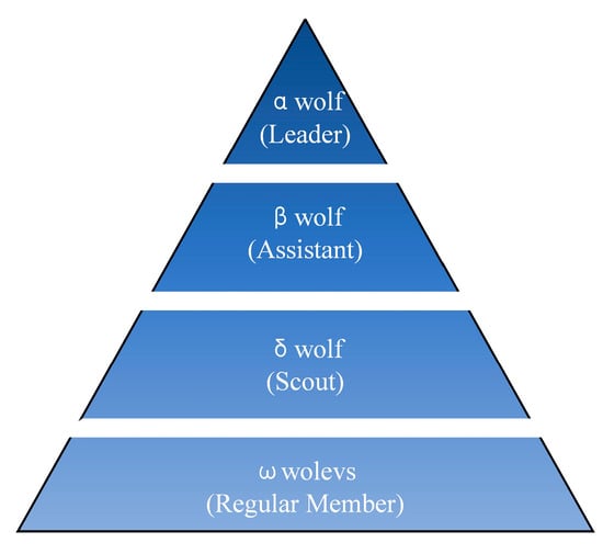
Figure 1. Grey wolf population hierarchy.

Assuming the search space is D-dimensional, and the number of grey wolves is N, the position vector of the n-th grey wolf at the t-th iteration is given by Equation (1):

$$X_n^t=\left[\begin{array}{cccc}{x}_1& x_2& \cdots & x_D\end{array}\right]$$

(1)

The fitness of every candidate solution (grey wolf) is determined by the objective function in each iteration. According to the fitness values, the top three best-performing grey wolves are selected as the α wolf, β wolf, and δ wolf, with their position vectors denoted as X_α, X_β, and X_δ, respectively. The remaining grey wolves are designated as ω wolves. The hunting (solving) process is guided by the top three wolves, while the remaining grey wolves move based on the positions of these three. When an individual grey wolf updates its position during the prey search, it must first calculate its distance to the currently selected α wolf, β wolf, and δ wolf using Equation (2):

$$\left\{\begin{array}{l}{D}_{\alpha }=\left|C_a\cdot X_{\alpha }-X_n^t\right|\\ D_{\beta }=\left|C_b\cdot X_{\beta }-X_n^t\right|\\ D_{\delta }=\left|C_c\cdot X_{\delta }-X_n^t\right|\end{array}\right.$$

(2)

where D_α, D_β, and D_δ represent the distances between the individual grey wolf and the current α wolf, β wolf, and δ wolf, respectively. C_a = 2$r_1$, C_b = 2$r_2$, and C_c = 2$r_3$, where $r_1$, $r_2$, and $r_3$ are random numbers between 0 and 1. These three coefficients are used to simulate the randomness in the movement of grey wolves around the prey.

According to distances to the current α wolf, β wolf, and δ wolf, the ω wolves adjust their movement (position update) during the hunting process to move closer to the prey. The position of the ω wolves is updated according to the position update formula shown in Equation (3):

$$\left\{\begin{array}{l}{X}_a=X_{\alpha }-A_a\cdot D_{\alpha }\\ X_b=X_{\beta }-A_b\cdot D_{\beta }\\ X_c=X_{\delta }-A_c\cdot D_{\delta }\\ X_n^{t+1}={\displaystyle \frac{X_a+X_b+X_c}{3}}\end{array}\right.$$

(3)

where X_a, X_b, and X_c represent the adjusted positions of the ω wolf influenced by the α, β, and δ wolves, respectively. The new position X_n^t+1 of the grey wolf is obtained by taking the average of these values. A_a, A_b, and A_c are a set of dynamic coefficients that determine the intensity and direction of the grey wolves’ movement toward the prey. The values of these three coefficients influence how closely the grey wolves encircle the prey, thereby affecting the exploratory and exploitative nature of the search behavior. The calculation method for A_a, A_b, and A_c is as follows:

$$\left\{\begin{array}{l}{A}_a=a\cdot (2r_4-1)\\ A_b=a\cdot (2r_5-1)\\ A_c=a\cdot (2r_6-1)\end{array}\right.$$

(4)

$$a=2\left(1-{\displaystyle \frac{t}{T}}\right)$$

(5)

In Equation (4), $r_4$, $r_5$, and $r_6$ are random numbers between 0 and 1, and a is the convergence factor. In Equation (5), T is the maximum iteration count, and t represents the current iteration number. The value of a decreases from 2 to 0 during the iteration process, simulating the behavior of grey wolves gradually closing in on their prey during the hunt. After each position update, when a dimension in the grey wolf’s position vector exceeds the search boundary, it is reinitialized using Equation (6):

$$x=\left(up-low\right)rand+low$$

(6)

where low is the lower boundary of the dimension, up is the upper boundary of the dimension, and rand is a random number within the range [0, 1].

When the maximum iteration count is reached, the position vector of the final α wolf is taken as the optimization result.

3. Balanced Grey Wolf Optimizer

To address the shortcomings of the traditional GWO, we propose improvements in two key aspects, resulting in a Balanced Grey Wolf Optimizer (BGWO) that incorporates a novel stochastic position update formula and a novel nonlinear convergence factor.

3.1. Selection of Benchmark Functions

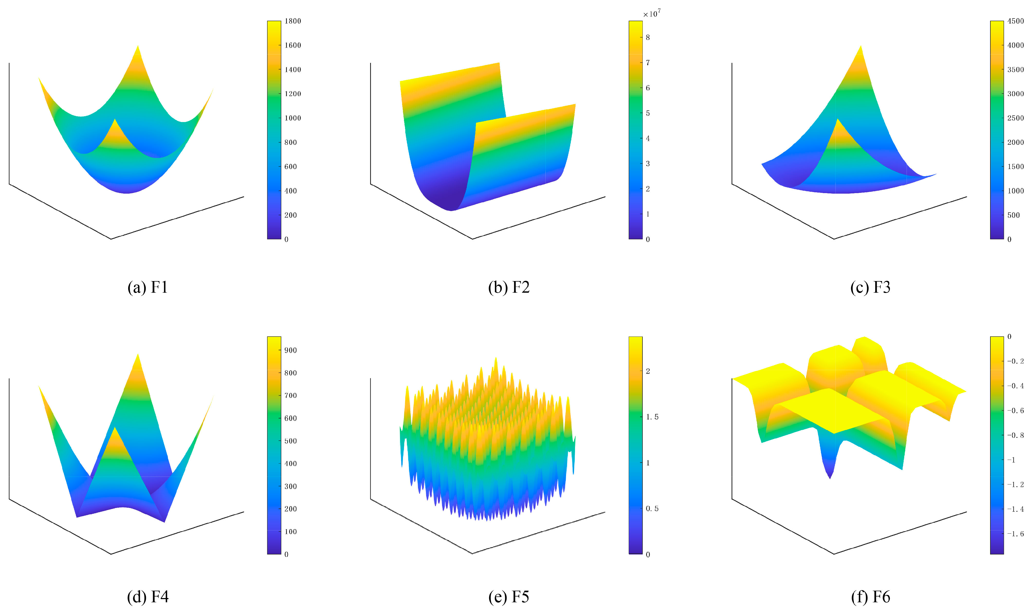
To evaluate the subsequently proposed BGWO, we first selected six commonly used benchmark functions. The information on these benchmark functions is presented in Table 1, and their distribution characteristics in three-dimensional space are illustrated in Figure 2. References [28,29] provide detailed descriptions of these benchmark functions. The functions we selected are representative to some extent. F1, F2, and F3 are unimodal functions, which effectively test the convergence of algorithms. F4, F5, and F6 exhibit multimodal characteristics, meaning they possess multiple local minima. These multimodal functions are particularly well-suited for evaluating the optimization algorithm’s local exploitation and global exploration capabilities.

Table 1. Benchmark functions.

Fun	Name	Multimodal	Mathematical Expression	Range	fmin
F1	Sphere	No	$f\left(x\right)={\displaystyle \sum _{i=1}^d{x}_i^2}$	[−30, 30]	0
F2	Rosenbrock	No	$f\left(x\right)={\displaystyle \sum _{i=1}^{d-1}[100{\left(x_{i+1}-x_i^2\right)}^2+{\left(x_i-1\right)}^2]}$	[−30, 30]	0
F3	Schwefel 1.2	No	$f\left(x\right)={\displaystyle \sum _{i=1}^d{\left({\displaystyle \sum _{j=1}^i{x}_j}\right)}^2}$	[−30, 30]	0
F4	Schwefel 2.22	Yes	$f\left(x\right)={\displaystyle \sum _{i=1}^d\left|x_i\right|}+{\displaystyle \prod _{i=1}^d\left|x_i\right|}$	[−30, 30]	0
F5	Griewank	Yes	$f\left(x\right)={\displaystyle \frac{1}{4000}}{\displaystyle \sum _{i=1}^d{x}_i^2}-{\displaystyle \prod _{i=1}^d\cos \left(\frac{x_i}{\sqrt{i}}\right)+1}$	[−600, 600]	0
F6	Michalewicz	Yes	$f\left(x\right)=-{\displaystyle \sum _{i=1}^d\sin \left(x_i\right)\cdot {\sin }^{20}\left(\frac{i{x}_i^2}{\pi }\right)}$	[0, π]	When d = 30, fmin = −29.63

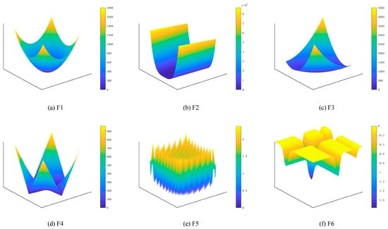
Figure 2. Images of benchmark functions in three-dimensional space.

3.2. Novel Stochastic Position Update Formula

In GWO, if the guiding roles of α, β, and δ wolves are overly dominant, it can easily lead to a premature convergence of the population. Fundamentally, excessive reliance on information from the leadership hierarchy during individual position updates causes rapid decay in population diversity. Under these conditions, premature convergence may trap the algorithm in local optima or result in the oversight of the global optimal solution.

To address the aforementioned issue, this paper modifies Equation (3) and proposes a novel stochastic position update formula. Its mathematical expression is shown in Equation (7):

$$\left\{\begin{array}{l}{X}_a=R_1\cdot \left(X_{\alpha }-A_a\cdot D_{\alpha }\right)\\ X_b=R_2\cdot \left(X_{\beta }-A_b\cdot D_{\beta }\right)\\ X_c=R_3\cdot \left(X_{\delta }-A_c\cdot D_{\delta }\right)\\ X_n^{t+1}={\displaystyle \frac{X_a+X_b+X_c}{3}}\end{array}\right.$$

(7)

where R₁, R₂, and R₃ are newly introduced random numbers designed to increase the randomness of the influence exerted by the leading wolves on other grey wolves. To prevent the random numbers from simultaneously taking the value of 0, which would cause the wolf pack to converge toward the origin, the range of these random numbers must be greater than 0. Therefore, in this paper, R₁, R₂, and R₃ in Equation (7) are set as random numbers within the interval [0.5, 1.5]. When one of these random numbers is less than 1, the influence of the corresponding leading wolf on the position update of the grey wolf individual is weakened; when the random number is greater than 1, the influence is enhanced. Since R₁, R₂, and R₃ are randomly and uniformly distributed within the interval [0.5, 1.5], the probabilities of enhancement and weakening are equal in the overall perspective. However, during each iteration, the same leading wolf exerts different degrees of positional influence on different grey wolf individuals. Therefore, the inclusion of these three random components mitigates the individuals’ overdependence on the leading wolves, thereby effectively slowing the decay of population diversity.

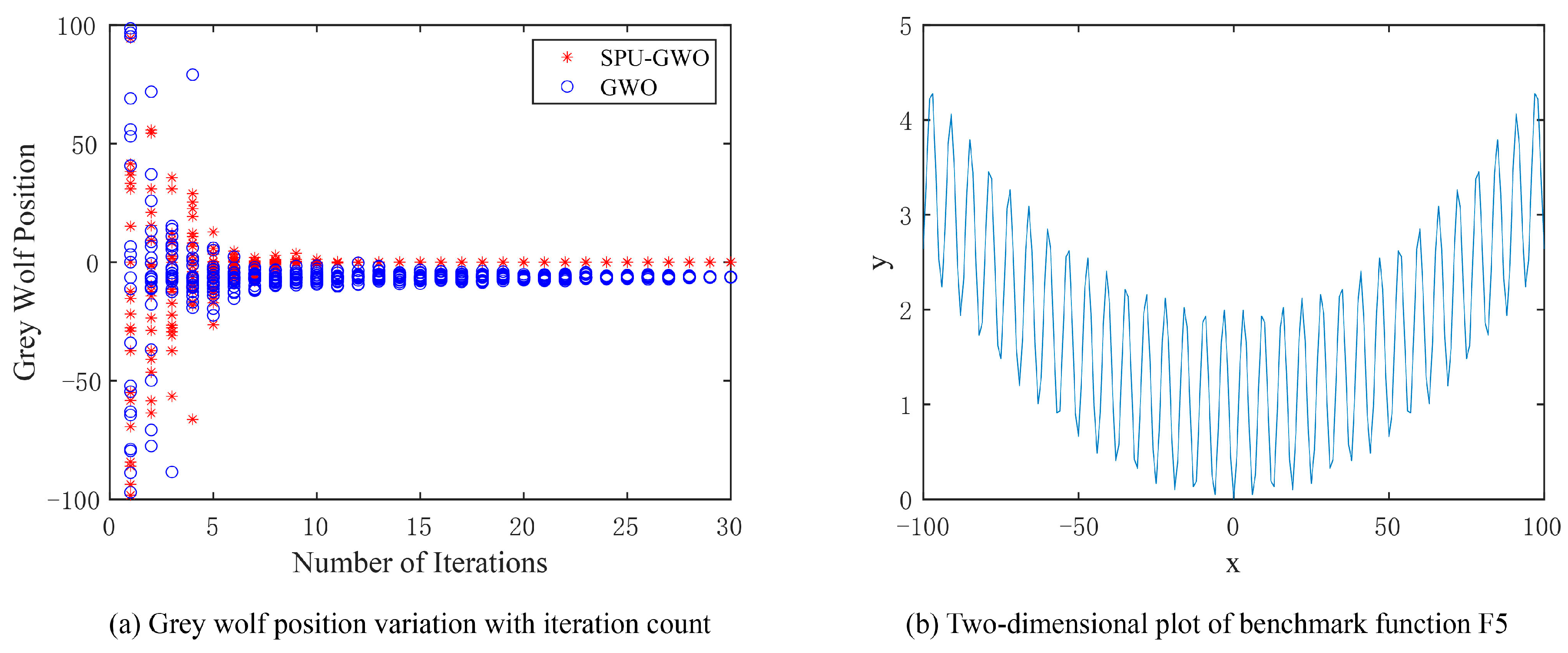
We used the multimodal functions F5 and F6 from the previous section to validate the optimization performance of the GWO using this stochastic position update formula (SPU-GWO). The number of iterations is set to 30, and the population size is set to 20. We illustrate trajectories in 1D for visualization; benchmark statistics are computed in D = 30, as specified below. For ease of observation, we set the search range for F5 to [−100, 100], while the search range for F6 is [−2π, 2π].

As shown in Figure 3b, the global minimum of F5 is 0, located at x = 0. The variation in grey wolf positions during the iterative optimization process for SPU-GWO and GWO is illustrated in Figure 3a. During the early stages of the search, the grey wolf population in GWO prematurely clustered and eventually converged to a local optimum near the global optimum of F5. In contrast, SPU-GWO maintained higher population diversity than GWO in the initial search phase and ultimately converged more accurately to the global optimum.

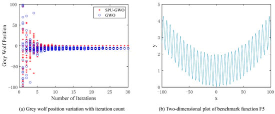
Figure 3. Variation in grey wolf positions while seeking the global minimum of the multimodal function F5.

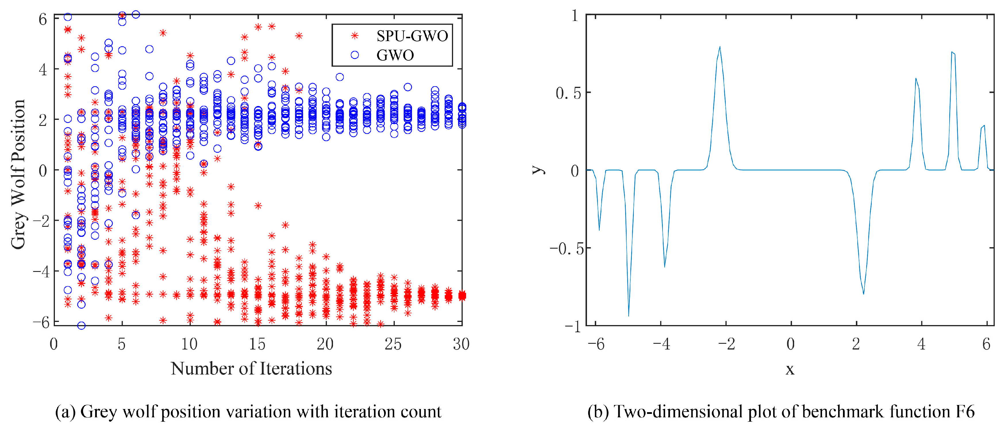
The two-dimensional plot of F6 is shown in Figure 4b. The 1D landscape suggests several local minima in the chosen range. The local minima are located at x = −5.88, x = −3.88, and x = 2.22, while the global minimum is at x = −4.98. The reported locations are verified numerically for the exact function definition and bounds. The variation in grey wolf positions during the search for the global minimum of F6 by SPU-GWO and GWO is depicted in Figure 4a. GWO prematurely converged to the local minimum at x = 2.22, indicating that it fell into a local optimum trap. In contrast, SPU-GWO correctly converged to the global minimum at x = −4.98. Furthermore, during the early stages of the search, the population position diversity of SPU-GWO is higher than that of GWO.

Figure 4. Variation in grey wolf positions while seeking the global minimum of the multimodal function F6.

The test results of benchmark functions F5 and F6 fully demonstrate that the SPU-GWO, which incorporates the stochastic position update formula, can prevent premature clustering of the wolf pack, thereby exhibiting stronger global search capabilities.

3.3. Novel Nonlinear Convergence Factor

The exploitation capability of the traditional GWO depends on the value of A_a, A_b, and A_c in Equation (4), and the values of A_a, A_b, and A_c are, in turn, influenced by the convergence factor a in Equation (5). The convergence factor of the traditional GWO decreases linearly from 2 to 0. Padhy et al. [30] demonstrated that such a linearly decreasing convergence factor fails to effectively distinguish between global search and local search. When using GWO for optimization, the search space is typically larger in the early stages, requiring rapid exploration. In contrast, as the search progresses and the prey is approached more closely, overly large step sizes can easily cause the algorithm to overshoot the search space and prematurely fall into local optima. Therefore, a more careful and precise search is needed in the later stages. To address the aforementioned issue with the linear convergence factor, this paper proposes a novel nonlinear convergence factor, whose mathematical expression is shown in Equation (8):

$$a={2\mathrm{e}}^{{\displaystyle \frac{k}{\ln \left(\frac{t-1}{T}\right)}}}$$

(8)

where t represents the current iteration number, k is the convergence coefficient of the convergence factor, and T is the maximum iteration count.

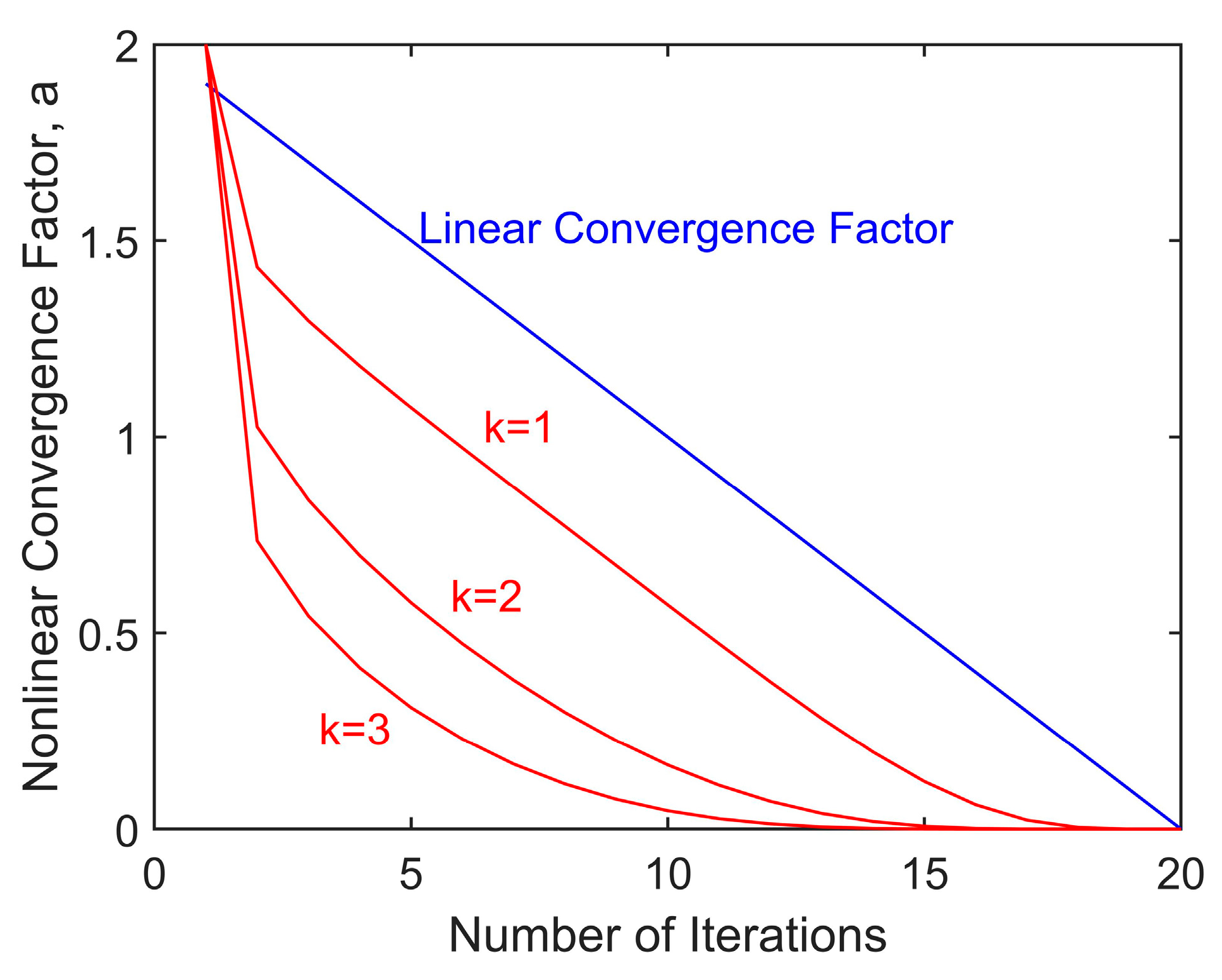
Given the complexity of the mathematical formulas for the nonlinear convergence factor a and its derivative, we will not conduct a detailed analysis of their mathematical properties. Instead, we will describe and discuss the characteristics of their variation through intuitive graphical representations. When the convergence coefficient k takes different values, the variation in a during the iteration process is shown in Figure 5. During the initial iterations, a decreases rapidly, enabling swift identification of potential extreme values during global search. In the later stages, the rate of decrease slows down, resulting in smaller search step sizes, which helps prevent missing the global optimum. Furthermore, it can be observed that a larger k value leads to a slighter decrease in a in the later stages.

Figure 5. Novel nonlinear convergence factor.

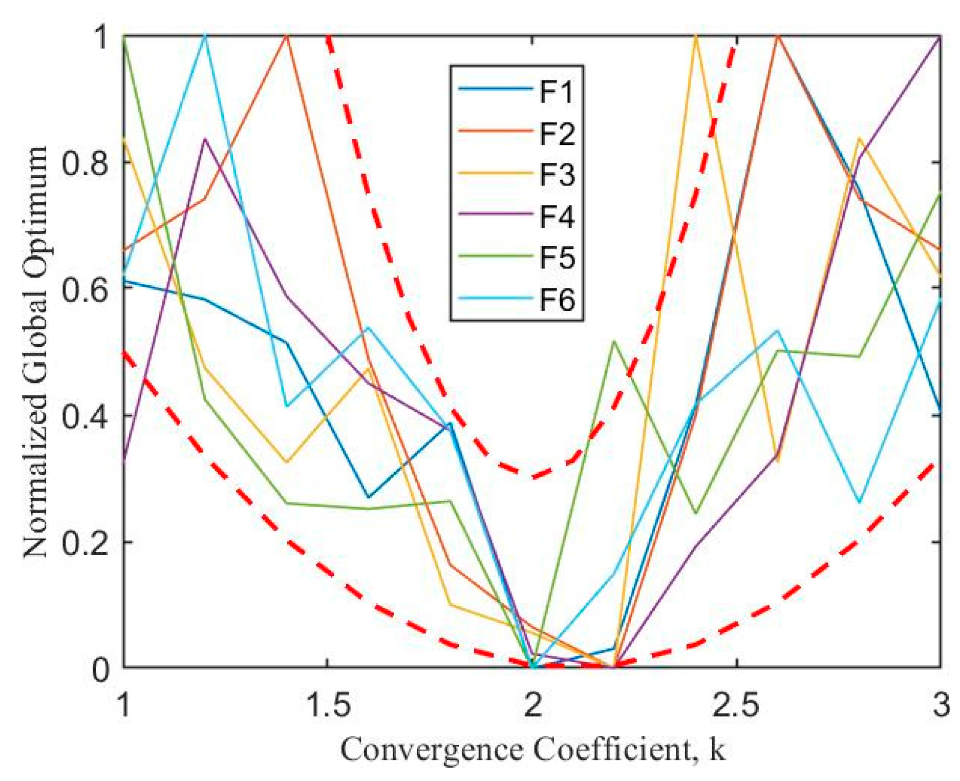
To balance rapid exploration in the initial phases and precise optimization in the later phases, k needs to be set to an appropriate value. To determine the most appropriate value of k, we tested the optimization performance of BGWO under different k values using six benchmark functions. For ease of comparison, we normalized the global optimal values of the benchmark functions under different k values according to Equation (9). The final results are shown in Figure 6. The figure indicates that the global optimum does not exhibit a definitive mathematical relationship with parameter k. However, overall, the graph exhibits characteristics of a quadratic function, with all benchmark functions achieving their minimum values around 2 and 2.2. Based on the above experimental results, this paper sets k to 2.2:

$$\mathrm{y}={\displaystyle \frac{x-x_{\min }}{x_{\max }-x_{\min }}}$$

(9)

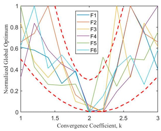
Figure 6. Optimization performance of BGWO on benchmark functions under different convergence coefficients.

3.4. Algorithm Performance Validation

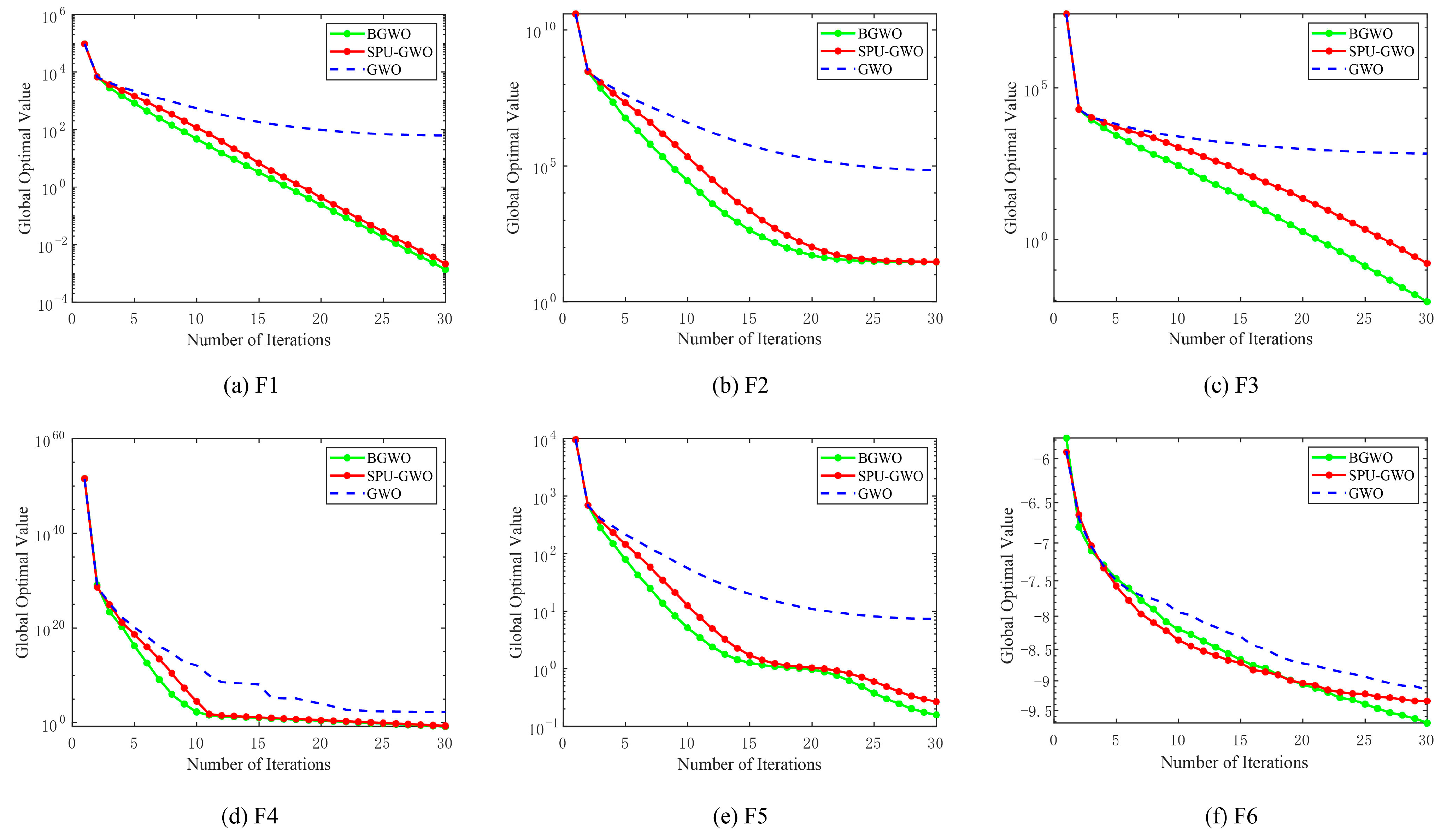
To validate that the improvements made to the GWO algorithm are effective, this paper utilizes the six benchmark functions in Table 1 as objective functions to test BGWO, GWO with only the stochastic position update formula (SPU-GWO), and the traditional GWO.

All convergence curves in Figure 7 are reported as the mean over 30 independent runs (same setting as Table 2).

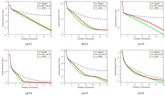
Figure 7. Benchmark function convergence curves under different algorithms.

Table 2. Test results under different algorithms.

Fun	Metric	BGWO	SPU-GWO	GWO
F1	MEAN	8.273 × 10−4	0.001	61.782
	STD	9.247 × 10−4	0.001	23.159
	Runtime (s)	0.046	0.040	0.043
F2	MEAN	28.932	29.187	7.002 × 104
	STD	0.0624	0.196	5.617 × 104
	Runtime (s)	0.038	0.035	0.035
F3	MEAN	0.006	0.092	680.283
	STD	0.005	0.119	241.96
	Runtime (s)	0.043	0.040	0.042
F4	MEAN	0.095	0.166	178.879
	STD	0.065	0.098	1.021 × 103
	Runtime (s)	0.046	0.042	0.044
F5	MEAN	0.143	0.247	7.305
	STD	0.351	0.367	2.131
	Runtime (s)	0.042	0.039	0.042
F6	MEAN	−9.723	−9.344	−9.178
	STD	1.242	0.870	0.846
	Runtime (s)	0.038	0.037	0.036

The maximum number of iterations for each algorithm is set to 30, the population size is set to 20, and the dimensionality of the search space is set to 30. To mitigate errors caused by random initialization of the population in each run, the standard deviation (STD) and the mean value (MEAN) from 30 independent runs of each algorithm are taken as comparative parameters.

The convergence curves of the benchmark functions are shown in Figure 7. It can be observed that BGWO and SPU-GWO demonstrate better convergence performance compared to GWO. For F3 and F6, the performance improvement of the algorithm is particularly evident after incorporating the nonlinear convergence factor. Since meta-heuristic algorithms evaluate multiple candidate solutions per iteration, their required computational budgets differ. Therefore, we calculated the average actual runtime for each algorithm over 30 independent runs. The programming tool used is MATLAB, and the CPU is an i5-8265U. The version of MATLAB we used is R2019b. As shown in Table 2, the runtime of each algorithm is very similar when tested on the same benchmark function. As shown in the table, the MEAN values of BGWO are lower than those of the other algorithms, indicating that BGWO can achieve better objective function values under the fixed iteration settings. Additionally, except for F6, the STDs of BGWO are also lower than those of the other algorithms, which further demonstrates that BGWO consistently attains results of similar precision across independent runs, highlighting its higher stability.

4. BPNN Based on BGWO

4.1. Construction of BGWO-BPNN

For a BPNN, since data sample spaces are often high-dimensional, multimodal, and contaminated by noise, training the weights and biases of a BPNN is considered a challenging optimization problem. BGWO is a heuristic algorithm, and a crucial step in training BPNNs using heuristic algorithms is selecting an appropriate encoding strategy. The purpose of choosing an encoding strategy is to represent the weights and biases of the BPNN as optimization variables for the heuristic algorithm. According to reference [31], encoding strategies can be categorized into three distinct types: vector encoding, matrix encoding, and binary encoding. Among these, vector encoding is particularly well-suited for training neural networks [32].

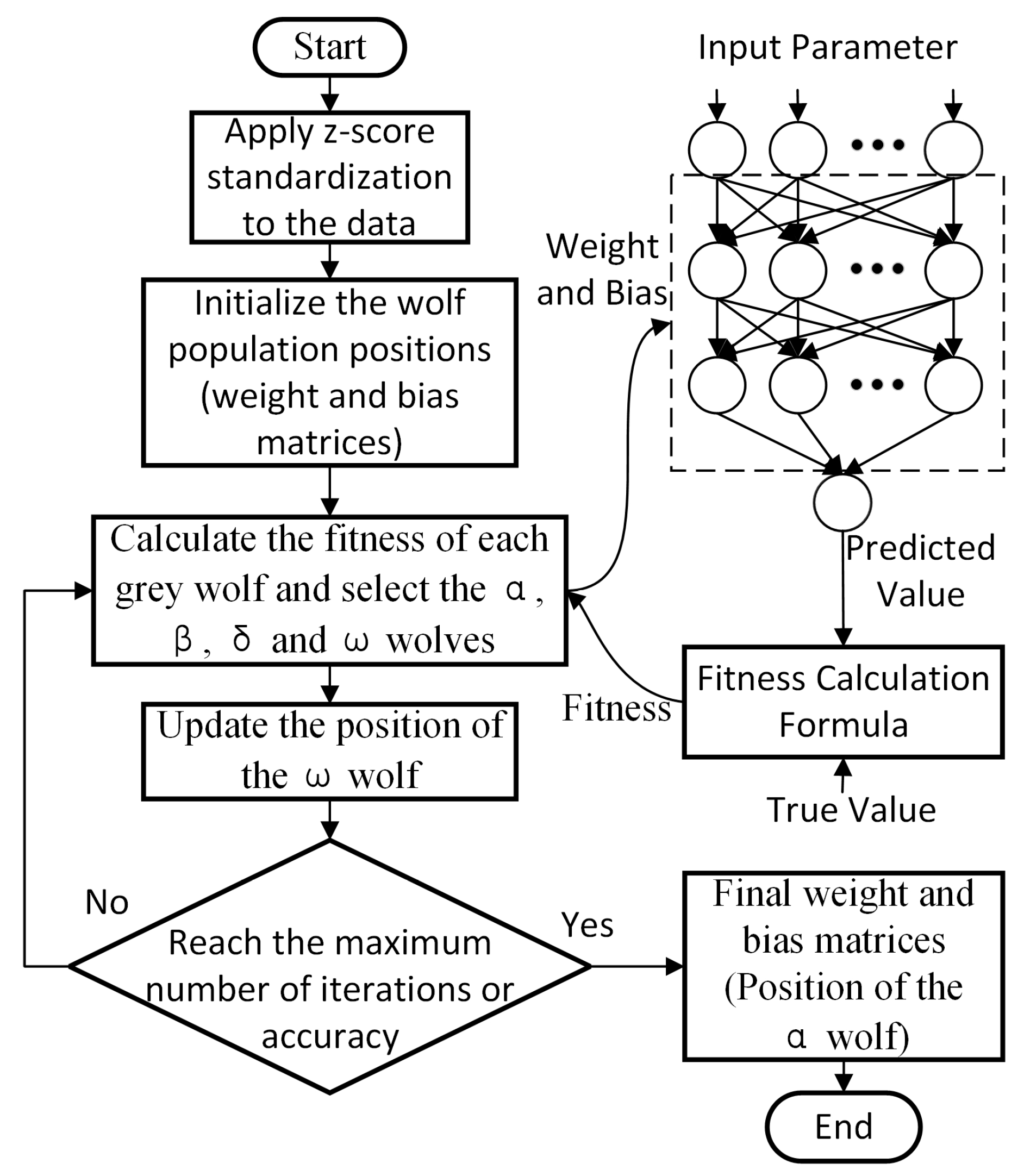
The implementation process of the vector encoding strategy is as follows: all weights and biases of the BPNN are expanded and concatenated into a one-dimensional vector W. The vector W is treated as the position vector of the GWO and is updated according to the methods described in Section 2 and Section 3. After the update is completed, the position vector is decoded back into the bias matrices and weight matrices of the BPNN. The fitness of the corresponding grey wolf is then calculated according to the current prediction output of the BPNN.

Based on the encoding strategy and Equation (1), this paper represents the weights and biases of a BPNN as the position vectors of the wolf pack in the BGWO during each iteration of training. The position vector is shown in Equation (10):

$$W_n^t=\left[\begin{array}{cccccccc}{w_{1,1}}^1& {w_{1,2}}^1& \cdots & {w_{i,j}}^{\mathrm{c}}& {{\theta }_1}^1& {{\theta }_2}^1& \cdots & {{\theta }_h}^c\end{array}\right]$$

(10)

where w_i,j^c represents the connection weight from the i-th neuron in the c-th layer to the j-th neuron in the (c + 1)-th layer. θ_h^c denotes the bias of the h-th neuron in the (c + 1)-th layer.

After defining the position vectors for the BGWO, it is also necessary to define the fitness function. The goal of training a BPNN is to input training samples into the network, utilize the BGWO for optimization to obtain appropriate weights and biases, and thereby enable the BPNN to achieve high approximation and prediction accuracy for the target problem. Therefore, the sum of squared differences between the actual output values of the BPNN and the expected output values is used as the fitness for the BGWO, serving as an indicator of the BPNN’s performance. The calculation formula for the fitness function is shown in Equation (11):

$$Fitness={\displaystyle \sum _{h=1}^{\mathrm{s}}{\displaystyle \sum _{i=1}^m{\left(o_i^h-d_i^h\right)}^2}}$$

(11)

where o_i^h represents the actual output value of the i-th output neuron when the network is fed with the h-th training sample; d_i^h denotes the expected output value of the i-th output neuron when the h-th training sample is applied; s indicates the number of training samples, and m is the number of output units in the BPNN.

In summary, the training process of the BGWO-based BPNN is illustrated in Figure 8.

Figure 8. Training process of BGWO-BPNN.

4.2. Test Results and Discussion

As shown in Table 3, this paper selected three public datasets—Abalone, Boston House Prices, and Energy Efficiency—to train and test the BPNN trained with BGWO (BGWO-BPNN), the BPNN trained with LM (LM-BPNN), and the traditional BPNN. These datasets and their detailed information can be obtained from the University of California, Irvine (UCI)’s Machine Learning Repository. The core characteristic of these datasets is the use of easily measurable physical or chemical attributes to predict a continuous variable that is difficult to obtain directly but holds significant value. These three widely used public tabular datasets are well-suited for training regression tasks. To adapt to the aforementioned three datasets, the network structure constructed in this paper is shown in Table 4. All BPNNs have no activation function in the Output Layer, while the activation functions for Hidden Layer 1 and Hidden Layer 2 are both the Tanh function. Its mathematical expression is shown in Equation (12):

$$\mathrm{Tanh}\left(x\right)={\displaystyle \frac{e^x-e^{-x}}{e^x+e^{-x}}}$$

(12)

Table 3. Public datasets.

Dataset Name	Input/Output	Metric
Abalone	Input Values	Sex, Length, Diameter, Height, Whole weight, Shucked weight, Viscera weight, Shell weight, and Rings
	Output Values	Age of the Abalone
Boston House Prices	Input Values	CRIM, ZN, INDUS, NOX, RM, AGE, DIS, RAD, TAX, PIRATIO, B, and LSTAT
	Output Values	Median House Price
Energy Efficiency	Input Values	Relative Compactness, Surface Area, Wall Area, Roof Area, Overall Height, Orientation, Glazing Area, and Glazing Area Distribution
	Output Values	Heating Load

Table 4. Neural network architecture.

Dataset	Number of Inputs	Number of Neurons in Hidden Layer 1	Number of Neurons in Hidden Layer 2	Number of Outputs
Abalone	9	6	5	1
Boston House Prices	12	8	7	1
Energy Efficiency	8	6	5	1

Random numbers in the range [0, 1] are generated using MATLAB’s rand function, with a fixed seed of 2 for reproducibility. We then assign these random numbers to each entry in the dataset and sort the data entries in ascending order according to these random numbers. The first 80% of each dataset is used for training, and the remaining 20% is used for testing. The parameter settings for each algorithm in BPNN training are shown in Table 5. Due to the fact that population-based algorithms evaluate multiple candidate solutions per iteration and the varying code complexities of different algorithms, to ensure a fair performance comparison among all algorithms, we have set the actual runtime for each algorithm to 3 s.

Table 5. Parameter settings for algorithms in BPNN training.

Algorithm	Parameter	Value
BGWO	Population Size	30
	Runtime (s)	3
LM	Learning Rate	10−5
	Runtime (s)	3
GD	Learning Rate	10−5
	Runtime (s)	3

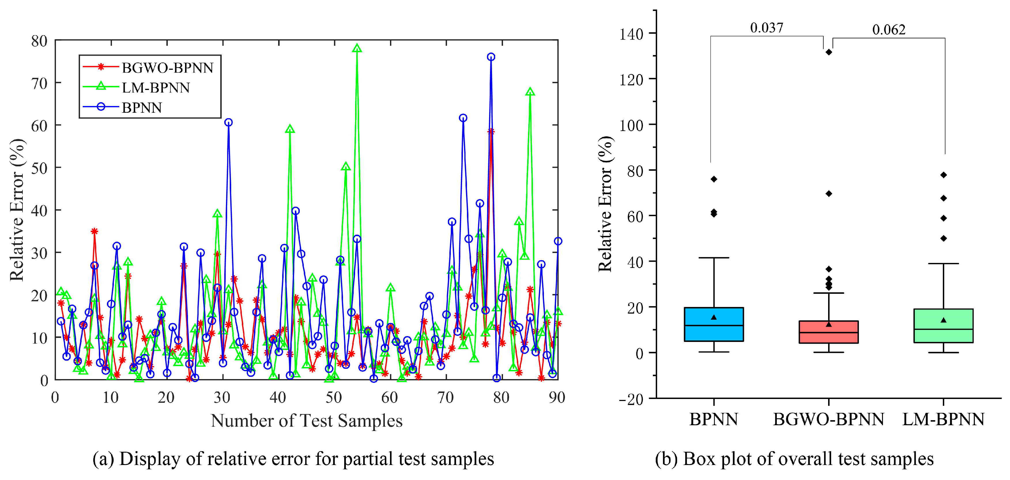
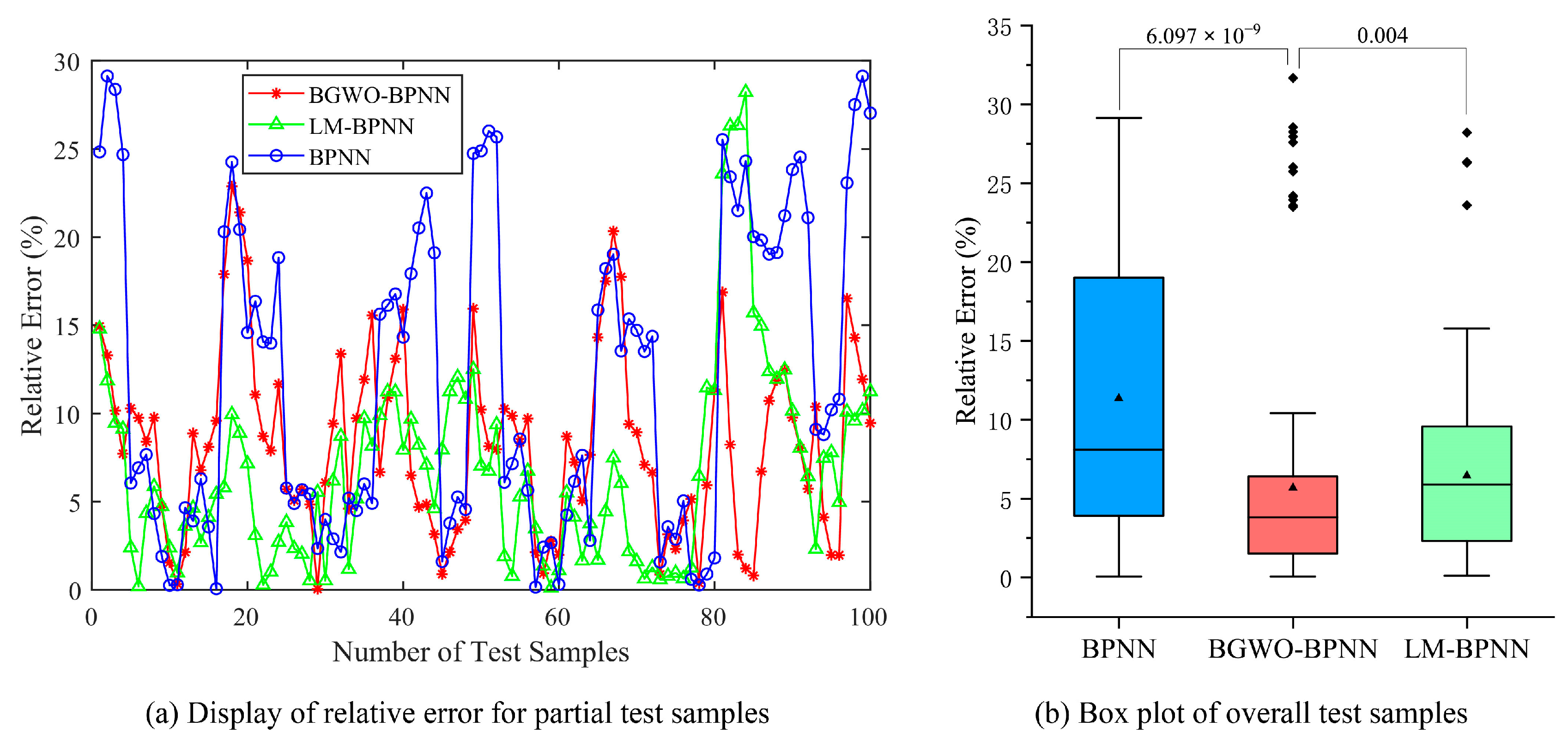
The test results for the three datasets are shown in Figure 9, Figure 10, and Figure 11, respectively. We also conduct the Wilcoxon test, and the results are displayed in the box plots from Figure 9, Figure 10 and Figure 11. The prediction error is defined as the relative error (RE), and its calculation method is given in Equation (13):

$$RE=\left|{\displaystyle \frac{P-D}{D}}\right|$$

(13)

where P is the predicted value of the BPNN, and D is the true value of the test sample.

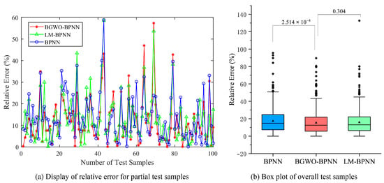
Figure 9. Test results for the Abalone dataset.

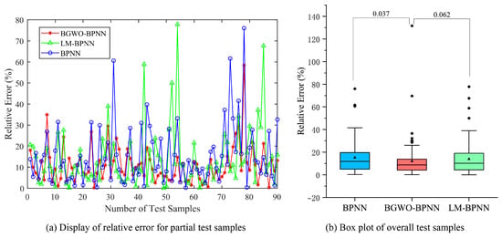
Figure 10. Test results for the Boston House Prices dataset.

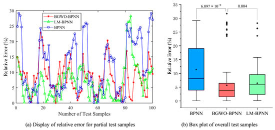
Figure 11. Test results for the Energy Efficiency dataset.

From the test results, BGWO-BPNN achieves smaller errors compared to LM-BPNN and the traditional BPNN. A significant difference is observed at the 5% level with respect to prediction performance, favoring BGWO-BPNN over the traditional BPNN in all experimental cases. There is a significant difference between BGWO-BPNN and LM-BPNN in the Energy Efficiency dataset.

To provide a more intuitive comparison of the predictive performance of the two neural networks, we calculated the mean absolute percentage error (MAPE) of the test samples for comparison. The method for calculating the MAPE is shown in Equation (14):

$$MAPE={\displaystyle \frac{1}{n}}{\displaystyle \sum _{i=1}^n\left|\frac{P_i-D_i}{D_i}\right|}\times 100\%$$

(14)

where D_i is the true value of the i-th test sample, P_i is the prediction of the BPNN for the i-th test sample, and n is the number of test samples.

The mean prediction errors are shown in Table 6. Compared to LM-BPNN, BGWO-BPNN achieves a certain reduction in MAPE. Compared to traditional BPNN, BGWO-BPNN achieves an absolute reduction in the MAPE for test samples of 1.976, 3.120, and 5.662 percentage points, respectively. Under the conditions established in this paper, BGWO shows certain competitiveness compared to LM and GD.

Table 6. Mean absolute percentage error comparison.

Dataset	Neural Network Type	MAPE	Absolute Reduction in Percentage Points Achieved by BGWO-BPNN
Abalone	BGWO-BPNN	15.397	0
	LM-BPNN	15.850	0.453
	BPNN	17.373	1.976
Boston House Prices	BGWO-BPNN	12.136	0
	LM-BPNN	13.922	1.786
	BPNN	15.256	3.120
Energy Efficiency	BGWO-BPNN	5.689	0
	LM-BPNN	6.462	0.773
	BPNN	11.351	5.662

5. Conclusions

To address issues such as susceptibility to poor local minima and slow convergence in traditional BPNNs, we present a Balanced Grey Wolf Optimizer as an alternative to the gradient descent method for training BPNNs. The key contributions of this work are summarized as follows:

(1)

This paper proposes a Balanced Grey Wolf Optimizer algorithm. First, we introduce a novel stochastic position update formula to reduce the dependence of the wolf pack on the leading wolves, thereby enhancing the global search capability of the GWO. Then, a novel nonlinear convergence factor is proposed, and the optimal convergence coefficient is explored, enabling GWO to achieve rapid exploration in the initial iterations and meticulous exploitation in the later iterations.

(2)

Six commonly used benchmark functions are selected as the objective functions to test the BGWO (which incorporates both the stochastic position update formula and the nonlinear convergence factor), the GWO with only the stochastic position update formula (SPU-GWO), and the traditional GWO. The test results validate that the BGWO demonstrates superior global exploration and local exploitation capabilities.

(3)

A BPNN training method based on the BGWO is constructed. Following the vector encoding strategy, the weights and biases in a BPNN are mapped to the position vectors of grey wolves in the BGWO, and the calculation method for the fitness function is provided. Finally, a complete BPNN training process is designed.

(4)

Three public datasets—Abalone, Boston House Prices, and Energy Efficiency—are selected to train and test BPNNs under different training methods. Furthermore, we use the Wilcoxon test to examine its significance. Under the experimental settings of this paper, the test results demonstrate an absolute reduction of 1.976, 3.120, and 5.662 percentage points in the MAPE achieved by BGWO-BPNN over the traditional BPNN. Compared to LM-BPNN, BGWO-BPNN also achieves a certain reduction in MAPE. This indicates that, under the conditions established in this paper, BGWO shows certain competitiveness compared to LM and GD.

In future research, the BGWO-BPNN will be applied in the fields of industry and control. BGWO will also be further improved and subsequently utilized for other optimization problems.

References

- Chen, S.; Cowan, C.; Grant, P. Orthogonal least squares learning algorithm for radial. IEEE Trans. Neural Netw. 1991, 2, 302–309. [Google Scholar] [CrossRef]
- Pollack, J. Recursive auto-associative memory: Devising compositional distributed representations. In Proceedings of the 10th Annual Conference Cognitive Science Society Pod, Portland, OR, USA, 11–14 August 2010; Taylor & Francis Group: Oxford, UK, 2019; pp. 33–39. [Google Scholar]
- LeCun, Y.; Bottou, L.; Bengio, Y.; Haffner, P. Gradient-based learning applied to document recognition. Proc. IEEE 2002, 86, 2278–2324. [Google Scholar] [CrossRef]
- Rumelhart, D.E.; Hinton, G.E.; Williams, R.J. Learning representations by back-propagating errors. Nature 1986, 323, 533–536. [Google Scholar] [CrossRef]
- Dauphin, Y.N.; Pascanu, R.; Gulcehre, C.; Cho, K.; Ganguli, S.; Bengio, Y. Identifying and attacking the saddle point problem in high-dimensional non-convex optimization. Adv. Neural Inf. Process Syst. 2014, 27, 1–14. [Google Scholar] [CrossRef]
- Bengio, Y.; Simard, P.; Frasconi, P. Learning long-term dependencies with gradient descent is difficult. IEEE Trans. Neural Netw. 1994, 5, 157–166. [Google Scholar] [CrossRef]
- Patrick, P. Minimisation methods for training feedforward Neural Networks. Neural Netw. 1994, 7, 1–11. [Google Scholar] [CrossRef]
- Gao, X.; Yang, F. A new method for training MLP neural networks. Chin. J. Comput. 1996, 9, 687–694. (In Chinese) [Google Scholar]
- Peng, S.; Fang, Z. The Joint optimization of BP Learning Algorithm. J. Circuits Syst. 2000, 5, 26–30, (In Chinese with English Abstract). [Google Scholar]
- Mirjalili, S. How effective is the Grey Wolf optimizer in training multi-layer perceptrons. Appl. Intell. 2015, 43, 150–161. [Google Scholar] [CrossRef]
- Leema, N.; Nehemiah, H.K.; Kannan, A. Neural network classifier optimization using differential evolution with global information and back propagation algorithm for clinical datasets. Appl. Soft Comput. 2016, 49, 834–844. [Google Scholar] [CrossRef]
- Zhang, R.; Tao, J. A nonlinear fuzzy neural network modeling approach using an improved genetic algorithm. IEEE Trans. Ind. Electron. 2017, 65, 5882–5892. [Google Scholar] [CrossRef]
- Xue, J.; Shen, B. A novel swarm intelligence optimization approach: Sparrow search algorithm. Syst. Sci. Control Eng. 2020, 8, 22–34. [Google Scholar] [CrossRef]
- Zhao, W.; Wang, L.; Zhang, Z. A novel atom search optimization for dispersion coefficient estimation in groundwater. Future Gener. Comput. Syst. 2019, 91, 601–610. [Google Scholar] [CrossRef]
- Dorigo, M.; Birattari, M.; Stützle, T. Ant colony optimization-artificial ants as a computational intelligence technique. IEEE Comput. Intell. Mag. 2006, 1, 28–39. [Google Scholar] [CrossRef]
- Tang, Y.; Cui, M.; Hua, C.; Li, L.; Yang, Y. Optimum design of fractional order PIλDμ controller for AVR system using chaotic ant swarm. Expert Syst. Appl. 2012, 39, 6887–6896. [Google Scholar] [CrossRef]
- Zhang, Y.; Huang, D.; Ji, M.; Xie, F. Image segmentation using PSO and PCM with Mahalanobis distance. Expert Syst. Appl. 2011, 38, 9036–9040. [Google Scholar] [CrossRef]
- Zou, D.; Gao, L.; Li, S.; Wu, J. An effective global harmony search algorithm for reliability problems. Expert Syst. Appl. 2011, 38, 4642–4648. [Google Scholar] [CrossRef]
- Mirjalili, S.; Mirjalili, S.M.; Lewis, A. Grey wolf optimizer. Adv. Eng. Softw. 2014, 69, 46–61. [Google Scholar] [CrossRef]
- Agarwal, J.; Parmar, G.; Gupta, R.; Sikander, A. Analysis of grey wolf optimizer based fractional order PID controller in speed control of DC motor. Microsyst. Technol. 2018, 24, 4997–5006. [Google Scholar] [CrossRef]
- Zhang, H.; Cai, Z.; Xiao, L.; Heidari, A.A.; Chen, H.; Zhao, D.; Wang, S.; Zhang, Y. Face image segmentation using boosted grey wolf optimizer. Biomimetics 2023, 8, 484. [Google Scholar] [CrossRef]
- Gan, W.; Zhou, X.; Wu, W.; Xu, C.-A. Research on the Optimization of Uncertain Multi-Stage Production Integrated Decisions Based on an Improved Grey Wolf Optimizer. Biomimetics 2025, 10, 775. [Google Scholar] [CrossRef]
- Cui, J.; Zhang, N.; Cui, X.; Wang, J.; Yu, M.; Liu, D.; Jiang, L. Fault diagnosis method of aircraft anti-skid brake system based on GWO-PNN. In Proceedings of the 2021 33rd Chinese Control and Decision Conference (CCDC), Kunming, China, 22–24 May 2021; pp. 5402–5406. [Google Scholar] [CrossRef]
- Zhou, L.; Yao, G. An Optimized GWO-BPNN Model for Predicting Corrosion Fatigue Performance of Stay Cables in Coastal Environments. J. Mar. Sci. Eng. 2024, 12, 2308. [Google Scholar] [CrossRef]
- Zhang, H.-T.; Yang, T.-T.; Wang, W.-T. A novel hybrid model for species distribution prediction using neural networks and Grey Wolf Optimizer algorithm. Sci. Rep. 2024, 14, 11505. [Google Scholar] [CrossRef]
- Luo, J.; Liu, Z. Novel grey wolf optimization based on modified differential evolution for numerical function optimization. Appl. Intell. 2020, 50, 468–486. [Google Scholar] [CrossRef]
- Nadimi-Shahraki, M.H.; Taghian, S.; Mirjalili, S. An improved grey wolf optimizer for solving engineering problems. Expert Syst. Appl. 2021, 166, 113917. [Google Scholar] [CrossRef]
- Simon, D. Biogeography-based optimization. IEEE Trans. Evol. Comput. 2008, 12, 702–713. [Google Scholar] [CrossRef]
- Wang, G.-G.; Deb, S.; Gandomi, A.H.; Zhang, Z.; Alavi, A.H. Chaotic cuckoo search. Soft Comput. 2016, 20, 3349–3362. [Google Scholar] [CrossRef]
- Padhy, S.; Panda, S.; Mahapatra, S. A modified GWO technique based cascade PI-PD controller for AGC of power systems in presence of Plug in Electric Vehicles. Eng. Sci. Technol. 2017, 20, 427–442. [Google Scholar] [CrossRef]
- Ali, M.H.; Al Mohammed, B.A.D.; Ismail, A.; Zolkipli, M.F. A new intrusion detection system based on fast learning network and particle swarm optimization. IEEE Access 2018, 6, 20255–20261. [Google Scholar] [CrossRef]
- Zhang, J.-R.; Zhang, J.; Lok, T.-M.; Lyu, M.R. A hybrid particle swarm optimization–back-propagation algorithm for feedforward neural network training. Appl. Math. Comput. 2007, 185, 1026–1037. [Google Scholar] [CrossRef]
Disclaimer/Publisher’s Note: The statements, opinions and data contained in all publications are solely those of the individual author(s) and contributor(s) and not of MDPI and/or the editor(s). MDPI and/or the editor(s) disclaim responsibility for any injury to people or property resulting from any ideas, methods, instructions or products referred to in the content. |
© 2026 by the authors. Licensee MDPI, Basel, Switzerland. This article is an open access article distributed under the terms and conditions of the Creative Commons Attribution (CC BY) license.