Stable and Efficient Gaussian-Based Kolmogorov–Arnold Networks

Abstract

Kolmogorov–Arnold Networks employ learnable univariate activation functions on edges rather than fixed node nonlinearities. Standard B-spline implementations require $O\left(3KW\right)$ parameters per layer (K basis functions, W connections). We introduce shared Gaussian radial basis functions with learnable centers ${\mu }_k^{\left(l\right)}$ and widths ${\sigma }_k^{\left(l\right)}$ maintained globally per layer, reducing parameter complexity to $O(KW+2LK)$ for L layers—a threefold reduction, while preserving Sobolev convergence rates $O\left(h^{s-\mathrm{\Omega }}\right)$. Width clamping at ${\sigma }_{min}={10}^{-6}$ and tripartite regularization ensure numerical stability. On MNIST with architecture $[784,128,10]$ and $K=5$, RBF-KAN achieves $87.8\%$ test accuracy versus $89.1\%$ for B-spline KAN with $1.4\times$ speedup and 33% memory reduction, though generalization gap increases from $1.1\%$ to $2.7\%$ due to global Gaussian support. Physics-informed neural networks demonstrate substantial improvements on partial differential equations: elliptic problems exhibit a $45\times$ reduction in PDE residual and maximum pointwise error, decreasing from $1.32$ to $0.18$; parabolic problems achieve a $2.1\times$ accuracy gain; hyperbolic wave equations show a $19.3\times$ improvement in maximum error and a $6.25\times$ reduction in $L^2$ norm. Superior hyperbolic performance derives from infinite differentiability of Gaussian bases, enabling accurate high-order derivatives without polynomial dissipation. Ablation studies confirm that coefficient regularization reduces mean error by 40%, while center diversity prevents basis collapse. Optimal basis count $K\in [3,5]$ balances expressiveness and overfitting. The architecture establishes Gaussian RBFs as efficient alternatives to B-splines for learnable activation networks with advantages in scientific computing.

1. Introduction

Modern neural network architectures face a fundamental trade-off between expressive power and computational efficiency. The capacity to approximate arbitrary continuous functions, formalized through the Universal Approximation Theorem [1,2,3,4], demands sufficient parameters to represent complex decision boundaries, yet excessive parameterization incurs prohibitive training costs and overfitting risks. Multilayer perceptrons (MLPs) address this challenge through depth and fixed activation functions (ReLU, Swish/SiLU, GELU [5,6]), but representational complexity remains proportional to network width, scaling as $O\left(W^2\right)$ for W connections per layer. Recurrent architectures mitigate temporal dependencies through memory mechanisms [7,8,9], while autoencoders achieve compact representations for dimensionality reduction [10,11] and data generation [12,13,14], yet all approaches fundamentally share the parameter scaling challenge. Kolmogorov–Arnold Networks (KANs) offer an alternative architectural paradigm wherein learnable univariate functions replace fixed activations, placing adaptability on network edges rather than nodes. Grounded in the Kolmogorov–Arnold representation theorem [15], KANs decompose multivariate functions into superpositions of univariate mappings, theoretically requiring exponentially fewer parameters than equivalent-capacity MLPs for low-dimensional smooth functions. While the original constructive proof yields fractal-like, nowhere differentiable universal functions unsuitable for practical computation, Liu et al. [16] introduced the first trainable KAN architecture by parameterizing univariate functions via B-spline basis expansions with adaptive grid refinement, achieving superior performance on symbolic regression and physics-informed neural network benchmarks. However, B-spline parameterization introduces two critical limitations that constrain practical scalability: (1) per-connection parameter overhead, each edge requires independent storage of $3K$ parameters (centers, widths, coefficients) for K basis functions, yielding total complexity $O\left(3KW\right)$ for a network with W connections; (2) polynomial smoothness constraints, while B-splines of order k possess only $C^{k-2}$ continuity, potentially introducing spurious numerical artifacts in applications requiring high-order derivatives, such as solving hyperbolic partial differential equations governed by wave propagation physics. This work addresses these limitations through a shared-basis architecture employing Gaussian radial basis functions (RBFs). Classical RBF networks have approximation-theoretic foundations, with universal approximation guarantees established by Park and Sandberg [17] and convergence rate analysis in Sobolev spaces provided by Schaback [18] and Wendland [19], demonstrating error decay scaling as $O\left(h^s\right)$, where s quantifies target function regularity and h represents fill distance. Gaussian RBFs provide $C^{\infty }$ smoothness, ensuring stable computation of arbitrarily high-order derivatives required for physics-informed applications. The infinite differentiability of Gaussian kernels proves particularly advantageous for hyperbolic PDEs, where exact representation of oscillatory solutions demands accurate higher-order spatial derivatives without polynomial truncation error. We introduce width clamping at threshold ${\sigma }_{min}={10}^{-6}$ combined with tripartite regularization to mitigate numerical conditioning pathologies inherent to RBF interpolation [20] while preserving approximation capacity. Theoretical analysis establishes that the shared-basis design maintains Sobolev space convergence rates $O\left(h^{s-\mathrm{\Omega }}\right)$ under mesh refinement, where $\mathrm{\Omega }$ represents domain dimensionality. The rest of this paper is structured as follows. Section 2 reviews related work on Kolmogorov–Arnold Networks, radial basis function approximation theory, and recent architectural innovations in learnable activation networks, positioning our contribution within the broader context of adaptive neural architectures. Section 3 establishes the mathematical foundations, including the Kolmogorov–Arnold representation theorem and Gaussian RBF approximation in Sobolev spaces. Section 4 presents the shared-basis RBF-KAN architecture, detailing the forward propagation algorithm and backpropagation with automatic differentiation for learnable centers and widths. Section 5 shows experimental validation on MNIST classification and three canonical physics-informed neural network benchmarks. Section 6 concludes with a discussion of trade-offs between parameter efficiency and generalization performance, limitations of global Gaussian support structures, and directions for future research, including hybrid local-global basis strategies and extensions to high-dimensional domains.

2. Related Work

The theoretical foundations of Kolmogorov–Arnold Networks originate from the representation theorem established independently by Kolmogorov [15] and Arnold [21], demonstrating that arbitrary continuous multivariate functions admit decomposition into superpositions of continuous univariate functions. While mathematically elegant, the constructive proof yields universal inner functions possessing fractal-like, nowhere differentiable structure unsuitable for practical computation [22,23]. Liu et al. [16] introduced the first trainable KAN architecture, parameterizing univariate activation functions via B-spline basis expansions with adaptive grid refinement, achieving superior parameter efficiency on symbolic regression and partial differential equation benchmarks compared with multilayer perceptrons of equivalent width.

Classical radial basis function networks constitute a well-established paradigm with rigorous approximation-theoretic foundations. Park and Sandberg [17] established universal approximation guarantees for Gaussian RBF networks under mild regularity conditions, while subsequent work by Schaback [18] and Wendland [19] provided convergence rate analysis in Sobolev spaces, demonstrating error decay scaling as $\mathcal{O}\left(h^s\right)$, where s denotes target function regularity and h represents fill distance. Buhmann [24] synthesized theoretical developments in his comprehensive monograph, establishing connections between RBF interpolation, kernel methods, and reproducing kernel Hilbert spaces. Numerical conditioning challenges inherent to Gaussian RBF interpolation have motivated stable algorithms incorporating variable basis placement and shape parameter optimization [20].

Recent architectural innovations in learnable activation networks include FastKAN [25], which replaces B-splines with rational function parameterizations to reduce computational overhead associated with grid operations, trading approximation fidelity against inference speed. Concurrent work has explored Chebyshev polynomial bases, Fourier features, and wavelet decompositions as alternative parameterization schemes, each offering distinct trade-offs between locality, smoothness, and computational efficiency. The broader context of adaptive activation functions encompasses PReLU [26], Swish/SiLU [5,6], and GELU [27], which learn scalar parameters modulating fixed nonlinearities rather than arbitrary univariate functions.

Physics-informed neural networks leverage automatic differentiation to embed differential equation constraints into loss functions, enabling mesh-free solution of forward and inverse problems [28,29,30]. The framework accommodates diverse equation types, including Navier-Stokes [31], Schrödinger [32], and Maxwell equations [33], with recent extensions addressing multi-scale phenomena [34], inverse design [35], and operator learning [36]. Theoretical analysis of PINN convergence properties remains active, with recent work establishing error bounds under regularity assumptions [37,38] and investigating failure modes in high-frequency or singularity-laden problems [39].

The neural tangent kernel framework introduced by Jacot et al. [40] provides analytical tools for studying infinite-width neural networks through kernel methods, establishing connections between gradient descent dynamics and kernel regression. Subsequent theoretical developments by Allen-Zhu et al. [41] and Du et al. [42] formalized global convergence guarantees under overparameterization, demonstrating exponential loss decay rates when the minimum eigenvalue of the NTK matrix remains bounded away from zero. Arora et al. [43] extended NTK analysis to finite-width networks, characterizing the lazy training regime where parameters remain near initialization throughout optimization.

The present contribution synthesizes these developments through a parameter-efficient shared-basis RBF-KAN architecture preserving approximation-theoretic guarantees while addressing computational tractability. Unlike the rational parameterization of FastKAN or the local B-spline support of the Standard KAN, the Gaussian RBF approach provides infinitely differentiable global basis functions naturally suited to physics-informed applications requiring high-order derivatives. The width regularization mechanism addresses conditioning pathologies inherent to RBF interpolation through gradient-based optimization with explicit stability constraints, avoiding classical techniques like variable shape parameter selection or greedy basis placement.

3. Mathematical Background

The theoretical foundation of Kolmogorov–Arnold Networks rests upon the fundamental representation theorem established independently by Kolmogorov and Arnold in 1957, which provides the conceptual basis for replacing traditional multilayer perceptrons with networks employing learnable univariate activation functions. We begin by recalling this classical result before developing the approximation-theoretic framework for Gaussian radial basis functions that underlies the proposed architectural design.

3.1. Kolmogorov–Arnold Representation Theorem

The possibility of representing arbitrary continuous multivariate functions through superpositions of continuous univariate functions was established through the following celebrated result.

Theorem 1

(Kolmogorov [15], Arnold [21]). Let $f:{[0,1]}^n\to \mathbb{R}$ be any continuous multivariate function. Then there exist continuous univariate functions ${\phi }_{q,p}:\mathbb{R}\to \mathbb{R}$ for $q=0,1,\dots ,2n$ and $p=1,2,\dots ,n$, and continuous outer functions ${\mathrm{\Phi }}_q:\mathbb{R}\to \mathbb{R}$ such that

$$f(x_1,x_2,\dots ,x_n)=\sum _{q=0}^{2n}{\mathrm{\Phi }}_q\left(\sum _{p=1}^n{\phi }_{q,p}\left(x_p\right)\right)$$

(1)

where the inner functions ${\left\{{\phi }_{q,p}\right\}}_{q,p}$ are universal in the sense that they depend only on the dimension n, not on the particular function f.

The proof of Theorem 1, while constructive, yields universal functions ${\phi }_{q,p}$ that are typically fractal-like, nowhere differentiable, and computationally intractable [22]. This structural understanding helps in creating practical neural network designs. A KAN with L layers and widths $n_0,n_1,\dots ,n_L$ implements a composite mapping $\mathcal{F}:{\mathbb{R}}^{n_0}\to {\mathbb{R}}^{n_L}$ through the recursive transformation

$$x_j^{(l+1)}=\sum _{i=1}^{n_l}{\phi }_{i,j}^{\left(l\right)}\left(x_i^{\left(l\right)}\right),j=1,2,\dots ,n_{l+1},l=0,1,\dots ,L-1$$

(2)

where ${\mathbf{x}}^{\left(l\right)}={(x_1^{\left(l\right)},x_2^{\left(l\right)},\dots ,x_{n_l}^{\left(l\right)})}^{\top }\in {\mathbb{R}}^{n_l}$ denotes the activation vector at layer l, and each ${\phi }_{i,j}^{\left(l\right)}:\mathbb{R}\to \mathbb{R}$ represents a learnable univariate function governing the connection from neuron i in layer l to neuron j in layer $l+1$.

The architectural distinction from conventional multilayer perceptrons is fundamental: whereas MLPs apply a fixed activation function $\sigma :\mathbb{R}\to \mathbb{R}$ uniformly across all neurons, KAN architectures learn connection-specific functions ${\phi }_{i,j}^{\left(l\right)}$ that can adapt to local input-output relationships. This flexibility necessitates the development of parameterization schemes that balance expressiveness with computational tractability. We address this challenge through Gaussian radial basis function expansions.

In more detail, radial basis functions provide a natural parameterization framework for univariate function approximation. A Gaussian radial basis function centered at $\mu \in \mathbb{R}$ with width parameter $\sigma \in {\mathbb{R}}_{+}=(0,\infty )$ is defined by

$$\psi (x;\mu ,\sigma )=exp\left(-{\displaystyle \frac{{(x-\mu )}^2}{2{\sigma }^2}}\right).$$

(3)

The universal approximation capability of Gaussian RBFs is established by the following classical result.

Theorem 2

(Park and Sandberg [17]). Let $\mathrm{\Omega }\subset \mathbb{R}$ be a compact set and let $f\in C\left(\mathrm{\Omega }\right)$ be continuous. For any $\epsilon >0$, there exist $N\in \mathbb{N}$, coefficients ${\left\{w_i\right\}}_{i=1}^N\subset \mathbb{R}$, centers ${\left\{{\mu }_i\right\}}_{i=1}^N\subset \mathbb{R}$, and shape parameters ${\left\{{\sigma }_i\right\}}_{i=1}^N\subset {\mathbb{R}}_{+}$ such that

$$\underset{x\in \mathrm{\Omega }}{sup}\left|f\left(x\right)-\sum _{i=1}^N{w}_{i}exp\left(-{\displaystyle \frac{{(x-{\mu }_i)}^2}{2{\sigma }_i^2}}\right)\right|<\epsilon .$$

(4)

Theorem 2 guarantees existence but provides no constructive guidance on the number of basis functions N required to achieve tolerance $\epsilon$, nor on the selection of centers and widths. In order to obtain quantitative convergence rates, we must impose regularity conditions on the target function and appeal to approximation theory in Sobolev spaces.

3.2. Approximation Theory in Sobolev Spaces

Throughout this paper, we adopt the convention

$$\hat{f}\left(\xi \right)={\int }_{\mathbb{R}}f\left(x\right)e^{-ix\xi }dx,f\left(x\right)={\displaystyle \frac{1}{2\pi }}{\int }_{\mathbb{R}}\hat{f}\left(\xi \right)e^{ix\xi }d\xi$$

(5)

for the Fourier transform and its inverse. Under this convention, Parseval’s identity takes the form

$${\parallel f\parallel }_{L^2\left(\mathbb{R}\right)}^2={\displaystyle \frac{1}{2\pi }}{\parallel \hat{f}\parallel }_{L^2\left(\mathbb{R}\right)}^2.$$

(6)

For integer regularity $s\in \mathbb{N}$, the Sobolev norm admits the equivalent definition

$${\parallel f\parallel }_{H^s\left(\mathrm{\Omega }\right)}={\left(\sum _{k=0}^s{\parallel f^{\left(k\right)}\parallel }_{L^2\left(\mathrm{\Omega }\right)}^2\right)}^{1/2},$$

(7)

where $f^{\left(k\right)}$ denotes the k-th weak derivative of f. The Sobolev norm for general $s>0$ is defined as

$${\parallel f\parallel }_{H^s\left(\mathbb{R}\right)}={\left({\displaystyle \frac{1}{2\pi }}{\int }_{\mathbb{R}}{(1+|\xi |}^2{)}^s{|\hat{f}\left(\xi \right)|}^{2}d\xi \right)}^{1/2}.$$

(8)

This Fourier-based definition (8) coincides with (7) when $s\in \mathbb{N}$ and provides a consistent extension to non-integer regularity indices. The Sobolev embedding theorem establishes the fundamental relationship between weak differentiability and pointwise continuity. By the Sobolev embedding theorem [44], functions in $H^s\left(\mathbb{R}\right)$ with $s>{\displaystyle \frac{1}{2}}$ admit continuous representatives with supremum norm controlled by ${\left|\right|f\left|\right|}_{H^s\left(\mathbb{R}\right)}.$

Theorem 3

(RBF Approximation on Compact Domains [19]). Let $\mathrm{\Omega }\subset \mathbb{R}$ be a compact interval and let $f\in H^s\left(\mathrm{\Omega }\right)$ be the restriction of a function in $H^s\left(\mathbb{R}\right)$ to Ω, with $s>1/2$. Let ${\left\{{\mu }_i\right\}}_{i=1}^N\subset \mathrm{\Omega }$ be a set of centers satisfying the quasi-uniformity condition: there exists a constant $c_{qu}\ge 1$ such that

$$h_{\mathrm{\Omega }}\le c_{qu}·\underset{i\ne j}{min}|{\mu }_i-{\mu }_j|$$

(9)

where the fill distance relative to Ω is defined as

$$h_{\mathrm{\Omega }}=\underset{x\in \mathrm{\Omega }}{sup}\underset{1\le i\le N}{min}|x-{\mu }_i|.$$

(10)

This quasi-uniformity condition ensures that centers are neither too clustered nor too sparse within Ω. Then there exists a Gaussian RBF interpolant of the form

$$I_{h_{\mathrm{\Omega }}}f\left(x\right)=\sum _{i=1}^N{\lambda }_{i}exp\left(-{\displaystyle \frac{{(x-{\mu }_i)}^2}{2{\sigma }^2}}\right)$$

(11)

with shape parameter $\sigma \asymp h_{\mathrm{\Omega }}$ (meaning there exist constants $0<c_1<c_2$ such that $c_1{h}_{\mathrm{\Omega }}\le \sigma \le c_2{h}_{\mathrm{\Omega }}$) as

$$\parallel f-I_{h_{\mathrm{\Omega }}}{f\parallel }_{L^2\left(\mathrm{\Omega }\right)}\le C{h}_{\mathrm{\Omega }}^s{\parallel f\parallel }_{H^s\left(\mathrm{\Omega }\right)}$$

(12)

where $C>0$ is a constant independent of f and $h_{\mathrm{\Omega }}$.

The proof is in the Appendix A.

The rate $\mathcal{O}\left(h_{\mathrm{\Omega }}^s\right)$ scales with target function regularity s, enabling rapid convergence for smooth functions with few basis functions.

3.3. Conditioning and Numerical Stability

While Theorem 3 establishes favorable approximation rates, practical implementation must contend with the ill-conditioning inherent in Gaussian RBF interpolation. Consider the interpolation problem on a compact domain $\mathrm{\Omega }$: given data ${\left\{(x_i,y_i)\right\}}_{i=1}^N$ with distinct points $x_1<x_2<\dots <x_N$ in $\mathrm{\Omega }$, find coefficients ${\left\{{\lambda }_i\right\}}_{i=1}^N$ such that

$$\sum _{j=1}^N{\lambda }_{j}exp\left(-{\displaystyle \frac{{(x_i-{\mu }_j)}^2}{2{\sigma }^2}}\right)=y_i,i=1,2,\dots ,N$$

(13)

where we take centers ${\mu }_j=x_j$ for simplicity. This yields the linear system $\mathbf{A}\mathbf{\lambda }=\mathbf{y}$ where the interpolation matrix $\mathbf{A}\in {\mathbb{R}}^{N\times N}$ has entries

$$A_{ij}=exp\left(-{\displaystyle \frac{{(x_i-x_j)}^2}{2{\sigma }^2}}\right).$$

(14)

The conditioning of $\mathbf{A}$ exhibits extreme sensitivity to the shape parameter $\sigma$ and the point distribution.

Theorem 4

(Conditioning of Gaussian RBF Matrices [18]). Let $\mathbf{A}\in {\mathbb{R}}^{N\times N}$ be the Gaussian RBF interpolation matrix (14) with uniformly spaced points $x_i=a+(i-1)h$ where $h>0$ is the uniform spacing on a bounded interval. Define the minimum separation $h_{min}={min}_{i\ne j}|x_i-x_j|=h$. Then the condition number satisfies the asymptotic bounds

$$\kappa \left(\mathbf{A}\right)={\displaystyle \frac{{\lambda }_{max}\left(\mathbf{A}\right)}{{\lambda }_{min}\left(\mathbf{A}\right)}}\sim \left\{\begin{array}{cc}\mathcal{O}\left({\sigma }^{-2N}\right)\hfill & as\sigma \to 0^{+}\hfill \\ \mathcal{O}\left(exp\left({\displaystyle \frac{C{\sigma }^2}{h^2}}\right)\right)\hfill & as\sigma \to +\infty \hfill \end{array}\right.$$

(15)

for a constant $C>0$ depending on the domain.

Theorem 4 reveals the fundamental trade-off in Gaussian RBF methods: small shape parameters $\sigma$ yield high-resolution approximations but severely ill-conditioned interpolation systems, while large $\sigma$ provides numerical stability at the cost of poor approximation quality. The optimal choice $\sigma \asymp h$ suggested by Theorem 3 attempts to balance these competing objectives, but even with this choice, condition numbers can become prohibitively large for dense point sets. However, we do not solve interpolation systems directly. Instead, we optimize the coefficients via gradient descent on a data-driven loss function. This optimization-based approach effectively mitigates conditioning issues through the following:

1.

Regularization: Penalty terms such as ${\lambda }_c{\sum }_k{c}_k^2$ improve effective conditioning by adding ${\lambda }_c\mathbf{I}$ to the Hessian of the loss, bounding the inverse curvature.

2.

Iterative refinement: Gradient descent naturally explores well-conditioned directions in parameter space, implicitly avoiding pathological subspaces associated with small singular values.

3.

Adaptive parameterization: Learning width parameters ${\sigma }_k$ individually for each basis function allows the network to automatically adjust widths to maintain numerical stability while preserving approximation power where needed.

Nevertheless, Theorem 4 underlines the importance of careful initialization and stabilization mechanisms, which we address through width clamping and regularization strategies.

3.4. Native Space Theory and Reproducing Kernel Hilbert Spaces

The Gaussian kernel $K(x,y;\sigma )=exp(-{(x-y)}^2/\left(2{\sigma }^2\right))$ induces a reproducing kernel Hilbert space (RKHS) ${\mathcal{H}}_K$, known as the native space of the kernel [19]. Functions in ${\mathcal{H}}_K$ can be represented as

$$f\left(x\right)=\sum _{i=1}^{\infty }{c}_{i}K(x,x_i;\sigma )$$

(16)

with coefficients satisfying ${\sum }_{i,j}{c}_i{c}_{j}K(x_i,x_j;\sigma )<\infty$. The native space norm is defined via

$${\parallel f\parallel }_{{\mathcal{H}}_K}^2=inf\left\{\sum _{i,j}{c}_i{c}_{j}K(x_i,x_j;\sigma ):f=\sum _i{c}_{i}K(·,x_i;\sigma )\right\}.$$

(17)

Given a discrete set of distinct points $X=\{x_1,\dots ,x_N\}$, the power function is defined as

$$P_{X,K}\left(x\right)=K(x,x;\sigma )-{\mathbf{k}}_X{\left(x\right)}^{\top }{\mathbf{K}}_X^{-1}{\mathbf{k}}_X\left(x\right)$$

(18)

where ${\mathbf{k}}_X\left(x\right)={(K(x,x_1;\sigma ),\dots ,K(x,x_N;\sigma ))}^{\top }\in {\mathbb{R}}^N$ and ${\mathbf{K}}_X\in {\mathbb{R}}^{N\times N}$ is the Gram matrix with entries ${\left({\mathbf{K}}_X\right)}_{ij}=K(x_i,x_j;\sigma )$. Given distinct points and the Gaussian kernel, ${\mathbf{K}}_X$ is strictly positive definite [19], hence invertible, ensuring that the power function is well-defined. The power function provides a pointwise error bound for RBF interpolation in the native space.

Theorem 5

(Pointwise Error Bound [19]). Let $f\in {\mathcal{H}}_K$ and let $I_{X}f$ denote the RBF interpolant to f at distinct points $X=\{x_1,\dots ,x_N\}$. Then for any $x\in \mathbb{R}$,

$$|f\left(x\right)-I_{X}f\left(x\right)|\le \sqrt{P_{X,K}\left(x\right)}{\parallel f\parallel }_{{\mathcal{H}}_K}.$$

(19)

The Theorem 5 suggests that approximation quality at a point x depends on both the native space norm of f and the power function $P_{X,K}\left(x\right)$. Considering well-distributed centers with fill distance $h_{\mathrm{\Omega }}$ in a compact domain $\mathrm{\Omega }$, the power function decays as $\mathcal{O}\left(h_{\mathrm{\Omega }}^{2s}\right)$ where s relates to the kernel smoothness, consistent with the $L^2$ convergence rate in Theorem 3.

3.5. Gaussian vs. B-Spline Basis Functions: Comparative Analysis

The choice between Gaussian RBF and B-spline parameterizations induces fundamental trade-offs in approximation capability, generalization behavior, and training dynamics. We establish a comparative analysis demonstrating that these basis function families occupy complementary architectural niches determined by their differing smoothness properties, support structures, and gradient characteristics. B-splines of order k are piecewise polynomials of degree $k-1$ with $C^{k-2}$ continuity at knot points. For the cubic B-spline parameterization ($k=3$) employed in Standard KAN experiments, the basis functions satisfy ${\psi }_{\text{B-spline}}\in C^1\left(\mathbb{R}\right)$, ensuring continuous first derivatives but exhibiting second-derivative discontinuities at knot locations. This limited smoothness constrains the regularity of network outputs $u_{\mathit{\theta }}$ composed through multiple layers, with derivative discontinuities accumulating at layer transitions. Conversely, Gaussian RBFs ${\psi }_{\mathrm{Gauss}}\left(x\right)=exp(-{(x-\mu )}^2/\left(2{\sigma }^2\right))$ belong to $C^{\infty }\left(\mathbb{R}\right)$, possessing continuous derivatives of all orders. This infinite differentiability ensures network outputs $u_{\mathit{\theta }}\in C^{\infty }$ regardless of network depth, enabling accurate automatic differentiation for arbitrary-order derivative computation. The practical consequence manifests in physics-informed neural network applications: hyperbolic wave equations require second-order mixed derivatives ${\partial }^{2}u/\partial t^2$ and ${\partial }^{2}u/\partial x^2$ in residual computation, and B-spline networks with $C^1$ regularity exhibit derivative discontinuities that corrupt these second-order terms, introducing numerical artifacts. Gaussian networks maintain ${\partial }^{2}u\in C^{\infty }$, explaining the 19.3× error reduction observed in the related section. The support structure differences between these basis families directly influence generalization behavior and computational efficiency. B-splines exhibit compact support determined by order k and grid spacing h, with cubic B-splines satisfying $\left|\mathrm{supp}\right({\psi }_{\text{B-spline}}\left)\right|=3h$. This locality ensures that perturbing basis parameters affects only function values within the compact support region, providing implicit regularization through limited parameter interaction. Each evaluation point interacts with at most k adjacent basis functions, yielding sparse Jacobian matrices and efficient gradient computation. In contrast, Gaussian RBFs exhibit global support with exponential decay characterized by the $ϵ$-effective support satisfying $|{\mathrm{supp}}_{ϵ}\left({\psi }_{\mathrm{Gauss}}\right)|=2\sigma \sqrt{2log(1/ϵ)}$. For numerical precision threshold $ϵ={10}^{-3}$ and $\sigma \asymp h$ (prescribed by Theorem 3 for optimal convergence), this yields an effective support width $7.4h$, substantially exceeding the B-spline support $3h$. Each evaluation point interacts with all K basis functions simultaneously, producing dense Jacobian matrices with increased computational overhead but enhanced expressiveness for global function features. After we establish that this global support amplifies effective model capacity from $d_{\mathrm{eff}}=O\left(1\right)$ for B-splines to $d_{\mathrm{eff}}=K$ for Gaussians. Classical learning theory predicts generalization gap scaling with $\sqrt{d_{\mathrm{eff}}}$, yielding factor $\sqrt{K}\approx 2.2$ amplification for $K=5$, consistent with observed ratio $(2.7\%/1.1\%)=2.45$ on MNIST. Considering smooth target functions $f\in H^s\left(\mathrm{\Omega }\right)$ with Sobolev regularity $s>k-2$, both B-splines and Gaussians achieve an asymptotic convergence rate of $O\left(h^s\right)$ under quasi-uniform basis placement (Theorem 3 for Gaussians, classical approximation theory for B-splines). However, pre-asymptotic behavior and suitability for different function classes differ substantially. B-splines efficiently represent functions with piecewise polynomial structure, achieving exact representation for polynomials of degree up to $k-1$ on each interval under appropriate conditions. For classification tasks with piecewise smooth decision boundaries, this efficiency manifests in superior MNIST accuracy (89.1% versus 87.8%). High-frequency sinusoidal functions $f\left(x\right)=sin\left(\omega x\right)$ with $\omega \gg 1$ require B-spline grid spacing $h\ll {\omega }^{-1}$ to adequately resolve oscillations, with approximation error scaling polynomially in $\omega h$. Gaussians with width $\sigma \sim {\omega }^{-1}$ naturally match the oscillation scale through their smooth exponential profile, achieving superior approximation for such functions. This advantage explains RBF-KAN performance on wave equation benchmarks (Section 5.2), where high-frequency components dominate solution structure and require accurate representation without introducing spurious numerical dissipation. The gradient behavior during optimization reflects these structural differences. For B-spline coefficient $c_i$, compact support yields gradient contributions only from samples within the support region $[t_i,t_{i+k}]$, producing sparse gradients with magnitude $O\left(\mathrm{local}\mathrm{batch}\mathrm{size}\right)$. For Gaussian center ${\mu }_k$, Theorem 8 establishes that all N samples in the batch contribute to the gradient through global support, yielding magnitude $O\left(N\right)$. This amplification necessitates learning rate adjustment: empirically, $\alpha ={10}^{-3}$ proves optimal for Gaussians under batch size $B=256$. For Gaussian width ${\sigma }_k$, Theorem 9 reveals a piecewise gradient structure with a vanishing derivative when clamping activates at ${\sigma }_k^2\le {ϵ}_{min}$. When unclamped, the gradient exhibits a cubic denominator ${\sigma }_k^{-3}$, inducing gradient explosion as ${\sigma }_k\to 0^{+}$. Width clamping at ${ϵ}_{min}={10}^{-6}$ (Section 4.2) prevents this pathology. B-spline knot parameters exhibit bounded gradients due to compact support, avoiding such instabilities. Global support Gaussians produce dense parameter interactions during optimization, wherein updating a single center ${\mu }_k$ affects loss contributions from all training samples.

3.6. Neural Tangent Kernel Perspective

Modern deep learning theory analyzes neural network optimization through the neural tangent kernel (NTK) framework [40]. For a network with parameters $\mathit{\theta }\in {\mathbb{R}}^P$ and output function $f_{\mathit{\theta }}:{\mathbb{R}}^d\to \mathbb{R}$, the neural tangent kernel at initialization is defined by

$$K_{\mathrm{NTK}}(x,x^{\prime };{\mathit{\theta }}_0)={〈{\nabla }_{\mathit{\theta }}{f}_{\mathit{\theta }}\left(x\right),{\nabla }_{\mathit{\theta }}{f}_{\mathit{\theta }}\left(x^{\prime }\right)〉}_{{\mathbb{R}}^P}{|}_{\mathit{\theta }={\mathit{\theta }}_0}.$$

(20)

In the case of overparameterized networks trained via gradient flow $d\mathit{\theta }/dt=-{\nabla }_{\mathit{\theta }}\mathcal{L}\left(\mathit{\theta }\right)$, the NTK remains approximately constant during training under certain conditions, and the training dynamics can be analyzed via kernel methods with $K=K_{\mathrm{NTK}}$.

Theorem 6

(NTK Convergence [40,41]). Consider gradient flow on the empirical squared loss

$$\mathcal{L}\left(\mathit{\theta }\right)={\displaystyle \frac{1}{2N}}\sum _{i=1}^N{(f_{\mathit{\theta }}\left(x_i\right)-y_i)}^2$$

(21)

where ${\left\{(x_i,y_i)\right\}}_{i=1}^N$ is a finite training set sampled i.i.d. from a distribution $\mathcal{D}$ over $\mathcal{X}\times \mathcal{Y}$, with initialization ${\mathit{\theta }}_0$. Assume the NTK matrix $\mathbf{K}\in {\mathbb{R}}^{N\times N}$ with entries $K_{ij}=K_{NTK}(x_i,x_j;{\mathit{\theta }}_0)$ satisfies $\mathbf{K}⪰{\lambda }_{min}\mathbf{I}$ for some ${\lambda }_{min}>0$. Then,

(i) The training loss converges exponentially:

$$\mathcal{L}\left(\mathit{\theta }\left(t\right)\right)\le \mathcal{L}\left({\mathit{\theta }}_0\right)exp(-2{\lambda }_{min}t).$$

(22)

(ii) The population risk satisfies

$${\mathbb{E}}_{(x,y)\sim \mathcal{D}}\left[{(f_{\mathit{\theta }\left(t\right)}\left(x\right)-y)}^2\right]-\underset{f\in {\mathcal{H}}_{NTK}}{inf}{\mathbb{E}}_{(x,y)\sim \mathcal{D}}\left[{(f\left(x\right)-y)}^2\right]=\mathcal{O}\left(\sqrt{{\displaystyle \frac{\mathrm{tr}\left({\mathbf{K}}^{-1}\right)}{N}}}\right)$$

(23)

where ${\mathcal{H}}_{NTK}$ denotes the RKHS associated with the kernel $K_{NTK}(·,·;{\mathit{\theta }}_0)$.

Considering RBF-based KAN architectures with learnable centers $\left\{{\mu }_k\right\}$ and widths $\left\{{\sigma }_k\right\}$, the NTK decomposes naturally according to parameter types. Denoting coefficients, centers, widths, and biases by $\mathbf{c},\mathit{\mu },\mathit{\sigma },\mathbf{b}$ respectively, the NTK admits the decomposition

$$K_{\mathrm{NTK}}(x,x^{\prime };{\mathit{\theta }}_0)=K_{\mathbf{c}}(x,x^{\prime };{\mathit{\theta }}_0)+K_{\mu }(x,x^{\prime };{\mathit{\theta }}_0)+K_{\sigma }(x,x^{\prime };{\mathit{\theta }}_0)+K_{\mathbf{b}}(x,x^{\prime };{\mathit{\theta }}_0)$$

(24)

where the kernel term for each parameter class $\mathbf{p}\in \{\mathbf{c},\mathit{\mu },\mathit{\sigma },\mathbf{b}\}$ is given by:

$$K_{\mathbf{p}}(x,x^{\prime };{\mathit{\theta }}_0)=〈{\nabla }_{\mathbf{p}}{f}_{\mathit{\theta }}\left(x\right),{\nabla }_{\mathbf{p}}{f}_{\mathit{\theta }}\left(x^{\prime }\right)〉{|}_{\mathit{\theta }={\mathit{\theta }}_0}.$$

The relative magnitudes of these terms depend on initialization scales and learning rates, providing insight into which parameters dominate the learning dynamics. In practice, coefficient parameters $\mathbf{c}$ typically contribute most significantly due to their large number and direct linear coupling to the output, while basis parameters $\mathit{\mu },\mathit{\sigma }$ play a secondary role in refining the feature representation.

4. Shared-Basis Architecture and Gradient Computation

Building upon the theoretical framework of the previous section, we develop a parameter-efficient RBF-KAN variant that reduces the parameter count from $\mathcal{O}\left(3KW\right)$ to $\mathcal{O}(KW+2LK)$ while preserving the approximation guarantees of Theorems 2 and 3. We provide complete gradient derivations and computational complexity analysis.

4.1. Architectural Design Principles

Classical implementations of RBF-KAN assign independent parameters $\{{\mu }_{i,j,k}^{\left(l\right)},{\sigma }_{i,j,k}^{\left(l\right)},c_{i,j,k}^{\left(l\right)}\}$ to each connection from neuron i in layer l to neuron j in layer $l+1$, indexed over each basis function $k\in \{1,\dots ,K\}$. This allocation yields $3K$ parameters per connection, resulting in a total parameter count of

$$\mathcal{O}\left(3K\sum _{l=0}^{L-1}{n}_l{n}_{l+1}\right)=\mathcal{O}\left(3KW\right),$$

(25)

where $W={\sum }_{l=0}^{L-1}{n}_l{n}_{l+1}$ denotes the aggregate number of connections across the network.

The convergence rate $\mathcal{O}\left(h_{\mathrm{\Omega }}^s\right)$ established in Theorem 3 depends fundamentally upon the collective distribution of basis centers throughout the domain, rather than upon connection-specific parameter assignments. This observation motivates a parameter-sharing strategy. Within each layer $l\in \{0,1,\dots ,L-1\}$, we introduce layer-wise global basis parameters:

$$\begin{array}{cc}\hfill {\mathit{\mu }}^{\left(l\right)}& ={({\mu }_1^{\left(l\right)},{\mu }_2^{\left(l\right)},\dots ,{\mu }_K^{\left(l\right)})}^{\top }\in {\mathbb{R}}^K,\hfill \\ \hfill {\mathit{\sigma }}^{\left(l\right)}& ={({\sigma }_1^{\left(l\right)},{\sigma }_2^{\left(l\right)},\dots ,{\sigma }_K^{\left(l\right)})}^{\top }\in {\mathbb{R}}_{+}^K,\hfill \end{array}$$

which define a shared feature map ${\mathbf{\Psi }}^{\left(l\right)}:\mathbb{R}\to {\mathbb{R}}^K$ given componentwise by

$${\mathrm{\Psi }}_k^{\left(l\right)}\left(x\right)=exp\left(-{\displaystyle \frac{{(x-{\mu }_k^{\left(l\right)})}^2}{2{\left({\sigma }_k^{\left(l\right)}\right)}^2}}\right),k=1,\dots ,K.$$

(26)

Under this parameterization, each connection $(i,j)$ between layers l and $l+1$ maintains exclusively a coefficient vector ${\mathbf{c}}_{i,j}^{\left(l\right)}={(c_{i,j,1}^{\left(l\right)},\dots ,c_{i,j,K}^{\left(l\right)})}^{\top }\in {\mathbb{R}}^K$. The learnable activation function associated with connection $(i,j)$ is then expressed as

$${\varphi }_{i,j}^{\left(l\right)}\left(x\right)=\langle {\mathbf{c}}_{i,j}^{\left(l\right)},{\mathbf{\Psi }}^{\left(l\right)}\left(x\right)\rangle =\sum _{k=1}^K{c}_{i,j,k}^{\left(l\right)}exp\left(-{\displaystyle \frac{{(x-{\mu }_k^{\left(l\right)})}^2}{2{\left({\sigma }_k^{\left(l\right)}\right)}^2}}\right).$$

(27)

The transformation is completed by introducing output bias terms ${\mathbf{b}}^{\left(l\right)}={(b_1^{\left(l\right)},b_2^{\left(l\right)},\dots ,b_{n_{l+1}}^{\left(l\right)})}^{\top }\in {\mathbb{R}}^{n_{l+1}}$ for each layer. This shared-basis design reduces the total parameter count to

$$\mathcal{O}\left(2KL+KW+n_{\mathrm{total}}\right)=\mathcal{O}\left(KW\right),$$

(28)

where $n_{\mathrm{total}}={\sum }_{l=1}^L{n}_l$ represents the total number of neurons. For networks with $K\ll 3$, this constitutes a substantial reduction in model complexity while preserving the approximation-theoretic guarantees of Theorem 3.

4.2. Convergence Rate Preservation Under Parameter Sharing

The parameter reduction from $O\left(3KW\right)$ to $O(KW+2LK)$ raises the question of whether shared-basis design degrades approximation-theoretic guarantees. We establish that the asymptotic Sobolev convergence rate $O\left(h_{\mathrm{\Omega }}^s\right)$ is preserved exactly under the assumption that all activation functions within a layer require similar basis support regions. We quantify the potential constant degradation when this assumption is violated.

Theorem 7

(Rate Preservation under Shared Support). Let $f\in H^s\left(\mathbb{R}\right)$ for $s>1/2$. Consider layer l with activation domain ${\mathrm{\Omega }}^{\left(l\right)}=[{\mu }_{min}^{\left(l\right)},{\mu }_{max}^{\left(l\right)}]$ representing the range of pre-activation values. Assume all connection-specific functions $\left\{{\varphi }_{i,j}^{\left(l\right)}\right\}$ require non-negligible values throughout ${\mathrm{\Omega }}^{\left(l\right)}$ (no extreme localization). Then:

(i) 

Shared-basis parameterization with K global centers ${\left\{{\mu }_k^{\left(l\right)}\right\}}_{k=1}^K$ quasi-uniformly distributed on ${\mathrm{\Omega }}^{\left(l\right)}$ achieves fill distance

$$h_{{\mathrm{\Omega }}^{\left(l\right)}}^{shared}={\displaystyle \frac{diam\left({\mathrm{\Omega }}^{\left(l\right)}\right)}{2(K-1)}}+O\left(K^{-2}\right).$$

(ii) 

Per-connection parameterization with independent centers ${\left\{{\mu }_{i,j,k}^{\left(l\right)}\right\}}_{k=1}^K$ quasi-uniformly distributed on ${\mathrm{\Omega }}^{\left(l\right)}$ achieves

$$h_{{\mathrm{\Omega }}^{\left(l\right)}}^{per\text{-}conn}={\displaystyle \frac{diam\left({\mathrm{\Omega }}^{\left(l\right)}\right)}{2(K-1)}}+O\left(K^{-2}\right)=h_{{\mathrm{\Omega }}^{\left(l\right)}}^{shared}.$$

(iii) 

Both interpolants satisfy identical convergence rates:

$$\parallel {\varphi }_{i,j}^{\left(l\right)}-I_{h_{\mathrm{\Omega }}}{\varphi }_{i,j}^{\left(l\right)}{\parallel }_{L^2\left({\mathrm{\Omega }}^{\left(l\right)}\right)}\le C{h}_{{\mathrm{\Omega }}^{\left(l\right)}}^s{\parallel {\varphi }_{i,j}^{\left(l\right)}\parallel }_{H^s\left({\mathrm{\Omega }}^{\left(l\right)}\right)}.$$

where the constant C depends on s and the quasi-uniformity constant $c_{qu}$ from Equation (8) but is independent of the parameter storage scheme.

Proof. 

Under the stated assumption that all connection functions $\left\{{\varphi }_{i,j}^{\left(l\right)}\right\}$ require non-negligible support throughout the common domain ${\mathrm{\Omega }}^{\left(l\right)}$, both parameterizations distribute K quasi-uniform basis functions over this domain. For quasi-uniform spacing with K points on interval $[a,b]$, the inter-point distance is $(b-a)/(K-1)$, yielding fill distance $(b-a)/\left(2\right(K-1\left)\right)$ since the worst-case point lies midway between consecutive centers. Thus, both achieve

$$h_{\mathrm{\Omega }}={\displaystyle \frac{{\mu }_{max}^{\left(l\right)}-{\mu }_{min}^{\left(l\right)}}{2(K-1)}}.$$

Theorem 3 establishes that for Gaussian RBF interpolation with quasi-uniform centers satisfying fill distance $h_{\mathrm{\Omega }}$ and shape parameter $\sigma \asymp h_{\mathrm{\Omega }}$, the $L^2$ error bound

$$\parallel f-I_{h_{\mathrm{\Omega }}}{f\parallel }_{L^2\left(\mathrm{\Omega }\right)}\le C(s,c_{\mathrm{qu}})h_{\mathrm{\Omega }}^s{\parallel f\parallel }_{H^s\left(\mathrm{\Omega }\right)}$$

holds with constant C depending on Sobolev regularity s and quasi-uniformity constant $c_{\mathrm{qu}}$, but independent of the specific center storage mechanism. Since both parameterizations achieve identical fill distance and satisfy identical quasi-uniformity conditions, they admit identical convergence rate exponent s.    □

Corollary 1

(Worst-Case Constant Degradation). If per-connection centers concentrate on a subdomain ${\mathrm{\Omega }}_{i,j}^{\left(l\right)}\subset {\mathrm{\Omega }}^{\left(l\right)}$ with $diam\left({\mathrm{\Omega }}_{i,j}^{\left(l\right)}\right)=\alpha ·diam\left({\mathrm{\Omega }}^{\left(l\right)}\right)$ for $\alpha \in (0,1]$, while shared-basis centers must cover the full domain ${\mathrm{\Omega }}^{\left(l\right)}$, then the fill distance ratio satisfies

$${\displaystyle \frac{h_{{\mathrm{\Omega }}^{\left(l\right)}}^{shared}}{h_{{\mathrm{\Omega }}_{i,j}^{\left(l\right)}}^{per\text{-}conn}}}={\displaystyle \frac{diam\left({\mathrm{\Omega }}^{\left(l\right)}\right)/\left(2(K-1)\right)}{\alpha ·diam\left({\mathrm{\Omega }}^{\left(l\right)}\right)/\left(2(K-1)\right)}}={\displaystyle \frac{1}{\alpha }}.$$

By Theorem 3, this induces constant degradation bounded by

$${\displaystyle \frac{C_{shared}}{C_{per\text{-}conn}}}\le {\alpha }^{-s}.$$

For $\alpha =0.5$ (per-connection centers specialized to half the global range) and Sobolev regularity $s=2$, this yields at most $4\times$ constant increase. Critically, the convergence rate exponent s remains identical regardless of α, confirming that parameter sharing affects only multiplicative constants, not asymptotic convergence behavior.

4.3. Numerical Stability via Width Parameter Regularization

The optimization of width parameters ${\sigma }_k^{\left(l\right)}\in {\mathbb{R}}_{+}$ presents inherent numerical challenges; in fact, as ${\sigma }_k^{\left(l\right)}\to 0^{+}$, gradient magnitudes diminish exponentially when $|x-{\mu }_k^{\left(l\right)}|\gg {\sigma }_k^{\left(l\right)}$, while concurrent evaluation of the exponential term $exp\left(-{\displaystyle \frac{{(x-{\mu }_k^{\left(l\right)})}^2}{2{\left({\sigma }_k^{\left(l\right)}\right)}^2}}\right)$ incurs risk of numerical overflow in the denominator. We mitigate these instabilities through a forward-pass regularization scheme that preserves unconstrained parameter evolution during optimization.

Definition 1

(Width Parameter Clamping). Given any layer index $l\in \{0,1,\dots ,L-1\}$ and basis function index $k\in \{1,\dots ,K\}$, we define the regularized squared width parameter by

$${\left({\hat{\sigma }}_k^{\left(l\right)}\right)}^2=max\{{\left({\sigma }_k^{\left(l\right)}\right)}^2,{\epsilon }_{min}\},$$

(29)

where ${\epsilon }_{min}={10}^{-6}$ denotes the minimum admissible squared width.

The evaluation of radial basis functions employs the regularized parameter ${\hat{\sigma }}_k^{\left(l\right)}$ in place of the native parameter ${\sigma }_k^{\left(l\right)}$:

$${\mathrm{\Psi }}_k^{\left(l\right)}\left(x\right)=exp\left(-{\displaystyle \frac{{(x-{\mu }_k^{\left(l\right)})}^2}{2{\left({\sigma }_k^{\left(l\right)}\right)}^2}}\right).$$

(30)

The stored parameters ${\left\{{\sigma }_k^{\left(l\right)}\right\}}_{k=1}^K$ remain unclamped throughout training and evolve according to standard gradient-based optimization; the regularization (29) is applied exclusively during forward propagation. This design prevents numerical pathologies while maintaining unrestricted exploration of the parameter manifold during optimization.

Lemma 1

(Uniform Boundedness of RBF Evaluations). Under the regularization scheme of Definition 1, the following properties hold uniformly over all $x\in \mathbb{R}$, all layers $l\in \{0,\dots ,L-1\}$, and all basis indices $k\in \{1,\dots ,K\}$:

(i)

$0<{\mathrm{\Psi }}_k^{\left(l\right)}\left(x\right)\le 1$;

(ii)

The exponential argument satisfies the bound

$$-{\displaystyle \frac{{(x-{\mu }_k^{\left(l\right)})}^2}{2{\left({\hat{\sigma }}_k^{\left(l\right)}\right)}^2}}\ge -{\displaystyle \frac{{(x-{\mu }_k^{\left(l\right)})}^2}{2{\epsilon }_{min}}}=-5\times {10}^5·{(x-{\mu }_k^{\left(l\right)})}^2.$$

(31)

Proof. 

Property (i): The upper bound follows from the non-positivity of the exponential argument. Since ${(x-{\mu }_k^{\left(l\right)})}^2\ge 0$ and ${\left({\hat{\sigma }}_k^{\left(l\right)}\right)}^2>0$, we obtain

$${\mathrm{\Psi }}_k^{\left(l\right)}\left(x\right)=exp\left(-{\displaystyle \frac{{(x-{\mu }_k^{\left(l\right)})}^2}{2{\left({\hat{\sigma }}_k^{\left(l\right)}\right)}^2}}\right)\le exp\left(0\right)=1.$$

The strict positivity ${\mathrm{\Psi }}_k^{\left(l\right)}\left(x\right)>0$ holds because the exponential function maps $\mathbb{R}$ into $(0,\infty )$.

Property (ii): By Definition 1, ${\left({\hat{\sigma }}_k^{\left(l\right)}\right)}^2\ge {\epsilon }_{min}$, which yields

$$-{\displaystyle \frac{{(x-{\mu }_k^{\left(l\right)})}^2}{2{\left({\hat{\sigma }}_k^{\left(l\right)}\right)}^2}}\ge -{\displaystyle \frac{{(x-{\mu }_k^{\left(l\right)})}^2}{2{\epsilon }_{min}}}.$$

Substituting ${\epsilon }_{min}={10}^{-6}$ gives

$$-{\displaystyle \frac{1}{2{\epsilon }_{min}}}=-{\displaystyle \frac{1}{2\times {10}^{-6}}}=-{\displaystyle \frac{{10}^6}{2}}=-5\times {10}^5.$$

Consider normalized inputs satisfying $\left|x\right|,|{\mu }_k^{\left(l\right)}|\le M$ with $M>0$. The triangle inequality ensures

$${(x-{\mu }_k^{\left(l\right)})}^2\le \left(\right|x|+|{\mu }_k^{\left(l\right)}{\left|\right)}^2\le 4M^2.$$

Taking $M=10$ as representative of standardized data yields ${(x-{\mu }_k^{\left(l\right)})}^2\le 400$, then

$$-{\displaystyle \frac{{(x-{\mu }_k^{\left(l\right)})}^2}{2{\epsilon }_{min}}}\ge -{\displaystyle \frac{400}{2\times {10}^{-6}}}=-2\times {10}^8,$$

which lies within the exponent range of IEEE 754 double-precision floating-point arithmetic (approximately $\pm {10}^{308}$), thereby guaranteeing numerical stability under standard computational implementations.    □

Dead unit prevention. When the width parameter ${\sigma }_k^{\left(l\right)}$ becomes sufficiently small such that ${\left({\sigma }_k^{\left(l\right)}\right)}^2\le {\epsilon }_{min}$, Theorem 9 establishes gradient vanishing $\partial \mathcal{L}/\partial {\sigma }_k^{\left(l\right)}=0$, creating a dead unit unable to adapt during optimization. The clamping mechanism prevents this pathology while inducing a singular Hessian structure at the boundary: for ${\left({\sigma }_k^{\left(l\right)}\right)}^2={\epsilon }_{min}$, the width Hessian entry satisfies ${\partial }^2\mathcal{L}/{(\partial {\sigma }_k^{\left(l\right)})}^2=0$ due to the vanishing first derivative, while off-diagonal coupling terms ${\partial }^2\mathcal{L}/(\partial {\sigma }_k^{\left(l\right)}\partial c_{i,j,k}^{\left(l\right)})$ remain nonzero via the chain rule through ${\mathrm{\Psi }}_{n,i,k}^{\left(l\right)}$ dependencies. This rank-deficient structure indicates that width parameters reaching ${\epsilon }_{min}$ effectively deactivate while coefficient parameters $c_{i,j,k}^{\left(l\right)}$ retain gradient flow. Empirically, initialization strategy (Equation (47)) with ${\sigma }_{\mathrm{init}}\approx ({\mu }_{max}-{\mu }_{min})/\left(2(K-1)\right)$ ensures all basis functions remain active throughout training, with observed minimum widths satisfying ${min}_k{\sigma }_k^{\left(l\right)}>{10}^{-3}=\sqrt{{\epsilon }_{min}}$ across all experiments.

Remark 1.

The regularization constant ${\epsilon }_{min}={10}^{-6}$ balances numerical stability against representational flexibility. Smaller values risk underflow in reciprocal computations, while larger values impose constraints on the expressivity of narrow basis functions.

4.4. Forward Propagation

We start by describing the forward propagation strategy. Let ${\mathbf{X}}^{\left(0\right)}\in {\mathbb{R}}^{B\times n_0}$ denote the input matrix containing B samples, where $X_{n,i}^{\left(0\right)}$ represents the i-th feature of the n-th sample. At layer $l\in \{0,1,\dots ,L-1\}$, we construct the evaluation tensor ${\mathbf{\Psi }}^{\left(l\right)}\in {\mathbb{R}}^{B\times n_l\times K}$ with entries defined by

$${\mathrm{\Psi }}_{n,i,k}^{\left(l\right)}=exp\left(-{\displaystyle \frac{{(X_{n,i}^{\left(l\right)}-{\mu }_k^{\left(l\right)})}^2}{2{\left({\hat{\sigma }}_k^{\left(l\right)}\right)}^2}}\right),$$

(32)

where indices range over $n\in \{1,\dots ,B\}$, $i\in \{1,\dots ,n_l\}$, and $k\in \{1,\dots ,K\}$. The coefficient structure is encoded in ${\mathbf{C}}^{\left(l\right)}\in {\mathbb{R}}^{n_l\times n_{l+1}\times K}$ with entries $C_{i,j,k}^{\left(l\right)}=c_{i,j,k}^{\left(l\right)}$. The activations at layer $l+1$ are computed via tensor contraction:

$$X_{n,j}^{(l+1)}=\sum _{i=1}^{n_l}\sum _{k=1}^K{\mathrm{\Psi }}_{n,i,k}^{\left(l\right)}{C}_{i,j,k}^{\left(l\right)}+b_j^{\left(l\right)},$$

(33)

where $n\in \{1,\dots ,B\}$ and $j\in \{1,\dots ,n_{l+1}\}$. In Einstein summation notation, this transformation takes the form

$${\mathbf{X}}^{(l+1)}=\mathtt{einsum}(’\mathrm{nik},\mathrm{ijk}\text{-}>\mathrm{nj}’,{\mathbf{\Psi }}^{\left(l\right)},{\mathbf{C}}^{\left(l\right)})+{\mathbf{1}}_B{\mathbf{b}}^{\left(l\right)\top },$$

(34)

where ${\mathbf{1}}_B\in {\mathbb{R}}^B$ denotes the vector of ones. Previous forward procedures are summarized in following Algorithm 1.

Algorithm 1 Shared-basis RBF-KAN forward propagation

Require: Input ${\mathbf{X}}^{\left(0\right)}\in {\mathbb{R}}^{B\times n_0}$, parameters ${\{{\mathit{\mu }}^{\left(l\right)},{\mathit{\sigma }}^{\left(l\right)},{\mathbf{C}}^{\left(l\right)},{\mathbf{b}}^{\left(l\right)}\}}_{l=0}^{L-1}$ Ensure: Output ${\mathbf{X}}^{\left(L\right)}\in {\mathbb{R}}^{B\times n_L}$   1: for$l=0,1,\dots ,L-1$do   2:     Compute ${\left({\hat{\sigma }}_k^{\left(l\right)}\right)}^2\leftarrow max\{{\left({\sigma }_k^{\left(l\right)}\right)}^2,{10}^{-6}\}$ over $k\in \{1,\dots ,K\}$   3:     Evaluate ${\mathbf{\Delta }}_{:,:,k}\leftarrow {\mathbf{X}}^{\left(l\right)}-{\mu }_k^{\left(l\right)}$ via broadcasting   4:     Compute ${\mathbf{\Psi }}_{:,:,k}^{\left(l\right)}\leftarrow exp\left(-{\mathbf{\Delta }}_{:,:,k}^{\odot 2}/\left(2{\left({\hat{\sigma }}_k^{\left(l\right)}\right)}^2\right)\right)$ over $k\in \{1,\dots ,K\}$   5:     Evaluate ${\mathbf{X}}^{(l+1)}\leftarrow \mathtt{einsum}(’\mathrm{nik},\mathrm{ijk}\text{-}>\mathrm{nj}’,{\mathbf{\Psi }}^{\left(l\right)},{\mathbf{C}}^{\left(l\right)})+{\mathbf{1}}_B{\mathbf{b}}^{\left(l\right)\top }$   6: end for     return ${\mathbf{X}}^{\left(L\right)}$

The computational complexity of each layer forward pass consists of two main operations. The radial basis function evaluation requires computing $B\times K\times n_l$ exponential functions, where B represents the batch size, K denotes the number of basis functions per dimension, and $n_l$ indicates the number of neurons in layer l. Each exponential function evaluation involves calculating the distance between input coordinates and basis function centers, followed by the exponential of the negative squared distance. The tensor contraction step then performs $B\times n_l\times n_{l+1}\times K$ multiply-accumulate operations, combining the evaluated basis functions with the learned weight tensor to produce the layer output. For each sample in the batch B, this operation maps $n_l$ input features to $n_{l+1}$ output features through K-dimensional basis function expansions, requiring element-wise multiplications followed by summations across all basis functions.

The total computational complexity of the forward pass scales as

$$T_{\mathrm{forward}}=\mathcal{O}\left(BWK\right),$$

(35)

where $W={\sum }_{l=0}^{L-1}{n}_l{n}_{l+1}$ denotes the total number of connections across the network.

4.5. Backward Propagation via Automatic Differentiation

We derive gradients with respect to all parameters $\mathit{\theta }={\{{\mathbf{C}}^{\left(l\right)},{\mathbf{b}}^{\left(l\right)},{\mathit{\mu }}^{\left(l\right)},{\mathit{\sigma }}^{\left(l\right)}\}}_{l=0}^{L-1}$ via reverse-mode automatic differentiation. Throughout this derivation, we assume the forward activations ${\{{\mathbf{X}}^{\left(l\right)},{\mathbf{\Psi }}^{\left(l\right)}\}}_{l=0}^{L-1}$ and the output gradient ${\displaystyle \frac{\partial \mathcal{L}}{\partial {\mathbf{X}}^{\left(L\right)}}}\in {\mathbb{R}}^{B\times n_L}$ are available from the forward pass and loss computation, respectively.

Lemma 2

(Coefficient Gradient). The linearity of the transformation (33) yields

$${\displaystyle \frac{\partial \mathcal{L}}{\partial C_{i,j,k}^{\left(l\right)}}}=\sum _{n=1}^B{\displaystyle \frac{\partial \mathcal{L}}{\partial X_{n,j}^{(l+1)}}}·{\mathrm{\Psi }}_{n,i,k}^{\left(l\right)}.$$

(36)

In tensor notation, this gradient admits the compact representation

$${\displaystyle \frac{\partial \mathcal{L}}{\partial {\mathbf{C}}^{\left(l\right)}}}=\mathtt{einsum}\left(’\mathit{nik},\mathit{nj}\text{-}>\mathit{ijk}’,{\mathbf{\Psi }}^{\left(l\right)},{\displaystyle \frac{\partial \mathcal{L}}{\partial {\mathbf{X}}^{(l+1)}}}\right).$$

(37)

Lemma 3

(Bias Gradient). The gradient with respect to the bias parameter $b_j^{\left(l\right)}$ is given by

$${\displaystyle \frac{\partial \mathcal{L}}{\partial b_j^{\left(l\right)}}}=\sum _{n=1}^B{\displaystyle \frac{\partial \mathcal{L}}{\partial X_{n,j}^{(l+1)}}}.$$

(38)

In vector form, this becomes

$${\displaystyle \frac{\partial \mathcal{L}}{\partial {\mathbf{b}}^{\left(l\right)}}}={\left({\displaystyle \frac{\partial \mathcal{L}}{\partial {\mathbf{X}}^{(l+1)}}}\right)}^{\top }{\mathbf{1}}_B.$$

We also establish the local derivatives of RBF evaluations before deriving the full loss gradients.

Lemma 4

(RBF Derivatives w.r.t. Basis Parameters). Let ${\mathrm{\Psi }}_k^{\left(l\right)}\left(x\right)=exp\left(-{\displaystyle \frac{{(x-{\mu }_k^{\left(l\right)})}^2}{2{\left({\hat{\sigma }}_k^{\left(l\right)}\right)}^2}}\right)$ denote the RBF evaluation. The following derivatives hold:

$$\begin{array}{cc}\hfill {\displaystyle \frac{\partial {\mathrm{\Psi }}_k^{\left(l\right)}\left(x\right)}{\partial {\mu }_k^{\left(l\right)}}}& ={\mathrm{\Psi }}_k^{\left(l\right)}\left(x\right)·{\displaystyle \frac{x-{\mu }_k^{\left(l\right)}}{{\left({\hat{\sigma }}_k^{\left(l\right)}\right)}^2}},\hfill \end{array}$$

(39)

$$\begin{array}{cc}\hfill {\displaystyle \frac{\partial {\mathrm{\Psi }}_k^{\left(l\right)}\left(x\right)}{\partial {\sigma }_k^{\left(l\right)}}}& =\left\{\begin{array}{cc}{\mathrm{\Psi }}_k^{\left(l\right)}\left(x\right)·{\displaystyle \frac{{(x-{\mu }_k^{\left(l\right)})}^2}{{\left({\sigma }_k^{\left(l\right)}\right)}^3}}\hfill & if{\left({\sigma }_k^{\left(l\right)}\right)}^2>{\epsilon }_{min},\hfill \\ 0\hfill & if{\left({\sigma }_k^{\left(l\right)}\right)}^2\le {\epsilon }_{min},\hfill \end{array}\right.\hfill \end{array}$$

(40)

$$\begin{array}{cc}\hfill {\displaystyle \frac{\partial {\mathrm{\Psi }}_k^{\left(l\right)}\left(x\right)}{\partial x}}& =-{\mathrm{\Psi }}_k^{\left(l\right)}\left(x\right)·{\displaystyle \frac{x-{\mu }_k^{\left(l\right)}}{{\left({\hat{\sigma }}_k^{\left(l\right)}\right)}^2}}.\hfill \end{array}$$

(41)

Proof. 

Equations (39) and (41) follow from the chain rule applied to the composite function $exp(-g(x\left)\right)$, where $g\left(x\right)={(x-{\mu }_k^{\left(l\right)})}^2/\left(2{\left({\hat{\sigma }}_k^{\left(l\right)}\right)}^2\right)$.

The piecewise structure of (40) arises from the clamping operation. When ${\left({\sigma }_k^{\left(l\right)}\right)}^2>{\epsilon }_{min}$, the regularized width satisfies ${\hat{\sigma }}_k^{\left(l\right)}={\sigma }_k^{\left(l\right)}$, and differentiating the exponential argument yields

$${\displaystyle \frac{\partial }{\partial {\sigma }_k^{\left(l\right)}}}\left[-{\displaystyle \frac{{(x-{\mu }_k^{\left(l\right)})}^2}{2{\left({\sigma }_k^{\left(l\right)}\right)}^2}}\right]={\displaystyle \frac{{(x-{\mu }_k^{\left(l\right)})}^2}{{\left({\sigma }_k^{\left(l\right)}\right)}^3}}.$$

Conversely, when ${\left({\sigma }_k^{\left(l\right)}\right)}^2\le {\epsilon }_{min}$, the clamping operation yields ${\hat{\sigma }}_k^{\left(l\right)}=\sqrt{{\epsilon }_{min}}$, which is constant with respect to ${\sigma }_k^{\left(l\right)}$, thereby producing a vanishing derivative. Complete derivations appear in Appendix A.    □

Theorem 8

(Center Parameter Gradient). The gradient of the loss function with respect to the center parameter ${\mu }_k^{\left(l\right)}$ is given by

$${\displaystyle \frac{\partial \mathcal{L}}{\partial {\mu }_k^{\left(l\right)}}}=\sum _{n=1}^B\sum _{i=1}^{n_l}\sum _{j=1}^{n_{l+1}}{\displaystyle \frac{\partial \mathcal{L}}{\partial X_{n,j}^{(l+1)}}}·C_{i,j,k}^{\left(l\right)}·{\displaystyle \frac{X_{n,i}^{\left(l\right)}-{\mu }_k^{\left(l\right)}}{{\left({\hat{\sigma }}_k^{\left(l\right)}\right)}^2}}·{\mathrm{\Psi }}_{n,i,k}^{\left(l\right)}.$$

(42)

Proof. 

Applying the chain rule yields

$${\displaystyle \frac{\partial \mathcal{L}}{\partial {\mu }_k^{\left(l\right)}}}=\sum _{n,i,j}{\displaystyle \frac{\partial \mathcal{L}}{\partial X_{n,j}^{(l+1)}}}·{\displaystyle \frac{\partial X_{n,j}^{(l+1)}}{\partial {\mathrm{\Psi }}_{n,i,k}^{\left(l\right)}}}·{\displaystyle \frac{\partial {\mathrm{\Psi }}_{n,i,k}^{\left(l\right)}}{\partial {\mu }_k^{\left(l\right)}}}.$$

From the forward transformation (33), we obtain ${\displaystyle \frac{\partial X_{n,j}^{(l+1)}}{\partial {\mathrm{\Psi }}_{n,i,k}^{\left(l\right)}}}=C_{i,j,k}^{\left(l\right)}$. Substituting the derivative (39) from Lemma 4 completes the derivation. The full calculation appears in Appendix A.    □

Theorem 9

(Width Parameter Gradient). The gradient with respect to the width parameter ${\sigma }_k^{\left(l\right)}$ admits the piecewise representation

$${\displaystyle \frac{\partial \mathcal{L}}{\partial {\sigma }_k^{\left(l\right)}}}=\left\{\begin{array}{cc}{\displaystyle \sum _{n=1}^B\sum _{i=1}^{n_l}\sum _{j=1}^{n_{l+1}}\frac{\partial \mathcal{L}}{\partial X_{n,j}^{(l+1)}}·C_{i,j,k}^{\left(l\right)}·\frac{{(X_{n,i}^{\left(l\right)}-{\mu }_k^{\left(l\right)})}^2}{{\left({\sigma }_k^{\left(l\right)}\right)}^3}·{\mathrm{\Psi }}_{n,i,k}^{\left(l\right)}}\hfill & if{\left({\sigma }_k^{\left(l\right)}\right)}^2>{\epsilon }_{min},\hfill \\ 0\hfill & if{\left({\sigma }_k^{\left(l\right)}\right)}^2\le {\epsilon }_{min}.\hfill \end{array}\right.$$

(43)

Proof. 

The result follows from applying the chain rule in conjunction with the derivative (40) from Lemma 4. The vanishing gradient when clamping is active establishes a soft lower bound on the width parameters during optimization.    □

Theorem 10

(Input Gradient). The gradient with respect to layer inputs, required for backpropagation to preceding layers, is given by

$${\displaystyle \frac{\partial \mathcal{L}}{\partial X_{n,i}^{\left(l\right)}}}=-\sum _{j=1}^{n_{l+1}}\sum _{k=1}^K{\displaystyle \frac{\partial \mathcal{L}}{\partial X_{n,j}^{(l+1)}}}·C_{i,j,k}^{\left(l\right)}·{\displaystyle \frac{X_{n,i}^{\left(l\right)}-{\mu }_k^{\left(l\right)}}{{\left({\hat{\sigma }}_k^{\left(l\right)}\right)}^2}}·{\mathrm{\Psi }}_{n,i,k}^{\left(l\right)}.$$

(44)

Proof. 

The chain rule with derivative (41) from Lemma 4 yields the stated expression. The negative sign reflects the translation symmetry of the Gaussian kernel: ${\displaystyle \frac{\partial \mathrm{\Psi }}{\partial x}}=-{\displaystyle \frac{\partial \mathrm{\Psi }}{\partial \mu }}$. The full derivation is in Appendix A.    □

The dominant operations at each layer consist of

• Coefficient gradients (line 4): $\mathcal{O}\left(B{n}_l{n}_{l+1}K\right)$ operations.
• Basis parameter gradients (lines 6–13): $\mathcal{O}(K·B{n}_l{n}_{l+1})=\mathcal{O}\left(B{n}_l{n}_{l+1}K\right)$ operations.
• Input gradients (lines 15–20): $\mathcal{O}(K·B{n}_l{n}_{l+1})=\mathcal{O}\left(B{n}_l{n}_{l+1}K\right)$ operations.

The total computational complexity of the backward pass scales as $T_{\mathrm{backward}}=\mathcal{O}\left(BWK\right)$, where $W={\sum }_{l=0}^{L-1}{n}_l{n}_{l+1}$ denotes the total connection count. The combined training cost per minibatch satisfies

$$T_{\mathrm{train}}=T_{\mathrm{forward}}+T_{\mathrm{backward}}=\mathcal{O}\left(BWK\right),$$

(45)

which matches the complexity of standard multilayer perceptrons up to a multiplicative factor of K (typically $K\in \{5,6,\dots ,10\}$ in practice). Forward procedures are shown in Algorithm 2.

Algorithm 2 Shared-basis RBF-KAN backpropagation
Require: Forward activations ${\{{\mathbf{X}}^{\left(l\right)},{\mathbf{\Psi }}^{\left(l\right)}\}}_{l=0}^{L-1}$, output gradient ${\displaystyle \frac{\partial \mathcal{L}}{\partial {\mathbf{X}}^{\left(L\right)}}}$
Ensure: Parameter gradients ${\left\{{\displaystyle \frac{\partial \mathcal{L}}{\partial {\mathbf{C}}^{\left(l\right)}}},{\displaystyle \frac{\partial \mathcal{L}}{\partial {\mathbf{b}}^{\left(l\right)}}},{\displaystyle \frac{\partial \mathcal{L}}{\partial {\mathit{\mu }}^{\left(l\right)}}},{\displaystyle \frac{\partial \mathcal{L}}{\partial {\mathit{\sigma }}^{\left(l\right)}}}\right\}}_{l=0}^{L-1}$
1: for  $l=L-1,L-2,\dots ,0$  do
2:    Compute ${\displaystyle \frac{\partial \mathcal{L}}{\partial {\mathbf{C}}^{\left(l\right)}}}\leftarrow \mathtt{einsum}(’\mathrm{nik},\mathrm{nj}\text{-}>\mathrm{ijk}’,{\mathbf{\Psi }}^{\left(l\right)},{\displaystyle \frac{\partial \mathcal{L}}{\partial {\mathbf{X}}^{(l+1)}}})$	▹ Coefficients
3:    Compute ${\displaystyle \frac{\partial \mathcal{L}}{\partial {\mathbf{b}}^{\left(l\right)}}}\leftarrow {\left({\displaystyle \frac{\partial \mathcal{L}}{\partial {\mathbf{X}}^{(l+1)}}}\right)}^{\top }{\mathbf{1}}_B$	▹ Biases
4:    Initialize ${\displaystyle \frac{\partial \mathcal{L}}{\partial {\mathbf{\mu }}^{\left(l\right)}}}\leftarrow \mathbf{0}\in {\mathbb{R}}^K$ and ${\displaystyle \frac{\partial \mathcal{L}}{\partial {\sigma }^{\left(l\right)}}}\leftarrow \mathbf{0}\in {\mathbb{R}}^K$
5:    for $k=1,2,\dots ,K$ do
6:        Evaluate ${\left({\hat{\sigma }}_k^{\left(l\right)}\right)}^2\leftarrow max\{{\left({\sigma }_k^{\left(l\right)}\right)}^2,{\epsilon }_{min}\}$
7:        Compute $\mathbf{G}\leftarrow {\displaystyle \frac{\partial \mathcal{L}}{\partial {\mathbf{X}}^{(l+1)}}}·{\left({\mathbf{C}}_{:,:,k}^{\left(l\right)}\right)}^{\top }$	▹ Weighted gradient
8:        Evaluate ${\mathbf{\Delta }}_{:,:,k}\leftarrow {\mathbf{X}}^{\left(l\right)}-{\mu }_k^{\left(l\right)}$
9:        Accumulate ${\displaystyle \frac{\partial \mathcal{L}}{\partial {\mu }_k^{\left(l\right)}}}\leftarrow {\sum }_{n,i}{G}_{n,i}·{\displaystyle \frac{{\mathrm{\Delta }}_{n,i,k}}{{\left({\hat{\sigma }}_k^{\left(l\right)}\right)}^2}}·{\mathrm{\Psi }}_{n,i,k}^{\left(l\right)}$	▹ Theorem 8
10:        if ${\left({\sigma }_k^{\left(l\right)}\right)}^2>{\epsilon }_{min}$ then
11:           Accumulate ${\displaystyle \frac{\partial \mathcal{L}}{\partial {\sigma }_k^{\left(l\right)}}}\leftarrow {\sum }_{n,i}{G}_{n,i}·{\displaystyle \frac{{\left({\mathrm{\Delta }}_{n,i,k}\right)}^2}{{\left({\sigma }_k^{\left(l\right)}\right)}^3}}·{\mathrm{\Psi }}_{n,i,k}^{\left(l\right)}$	▹ Theorem 9
12:        end if
13:    end for
14:    if $l>0$ then	▹ Input gradients when not at input layer
15:        Initialize ${\displaystyle \frac{\partial \mathcal{L}}{\partial {\mathbf{X}}^{\left(l\right)}}}\leftarrow \mathbf{0}\in {\mathbb{R}}^{B\times n_l}$
16:        for $k=1,\dots ,K$ do
17:           Compute ${\mathbf{G}}_k\leftarrow {\displaystyle \frac{\partial \mathcal{L}}{\partial {\mathbf{X}}^{(l+1)}}}·{\left({\mathbf{C}}_{:,:,k}^{\left(l\right)}\right)}^{\top }$
18:           Evaluate ${\mathbf{\Delta }}_{:,:,k}\leftarrow {\mathbf{X}}^{\left(l\right)}-{\mu }_k^{\left(l\right)}$
19:           Accumulate ${\displaystyle \frac{\partial \mathcal{L}}{\partial {\mathbf{X}}^{\left(l\right)}}}\leftarrow {\displaystyle \frac{\partial \mathcal{L}}{\partial {\mathbf{X}}^{\left(l\right)}}}-{\mathbf{G}}_k\odot {\displaystyle \frac{{\mathbf{\Delta }}_{:,:,k}}{{\left({\hat{\sigma }}_k^{\left(l\right)}\right)}^2}}\odot {\mathbf{\Psi }}_{:,:,k}^{\left(l\right)}$	▹ Negative sign, Theorem 10
20:        end for
21:    end if
22:end for

4.6. Initialization, Optimization, and Stability

Having established the forward and backward propagation algorithms, we now specify the complete training framework. This includes the geometric initialization strategy based on Theorem 3, the differentiated optimization protocol with adaptive learning rates matched to the gradient scaling established in Theorems 8 and 9, and the regularized objective function that enforces desirable properties during training. We conclude with theoretical stability guarantees ensuring well-conditioned optimization dynamics.

4.6.1. Parameter Initialization Strategy

We adopt a geometric initialization scheme based on the approximation-theoretic principles established in Theorem 3. The centers ${\left\{{\mu }_k^{\left(l\right)}\right\}}_{k=1}^K$ are distributed uniformly over the expected activation range $[{\mu }_{min},{\mu }_{max}]=[-2.5,2.5]$ according to

$${\mu }_k^{\left(l\right)}={\mu }_{min}+{\displaystyle \frac{{\mu }_{max}-{\mu }_{min}}{K-1}}(k-1),k\in \{1,\dots ,K\}.$$

(46)

Meanwhile, all widths are initialized uniformly at ${\sigma }_k^{\left(l\right)}={\sigma }_{\mathrm{init}}$, where

$${\sigma }_{\mathrm{init}}\approx {\displaystyle \frac{{\mu }_{max}-{\mu }_{min}}{2(K-1)}}.$$

(47)

This choice yields moderate overlap between adjacent basis functions, consistent with the optimal scaling $\sigma \asymp h_{\mathrm{\Omega }}$ prescribed by Theorem 3, where the characteristic mesh size satisfies

$$h_{\mathrm{\Omega }}=({\mu }_{max}-{\mu }_{min})/(K-1).$$

Regarding coefficients parameters, we employ a target-guided warm-start strategy that approximates a reference activation function $g:\mathbb{R}\to \mathbb{R}$ (typically ReLU or GELU):

$$c_{i,j,k}^{\left(l\right)}=g\left({\mu }_k^{\left(l\right)}\right)+{\alpha }_{\mathrm{init}}·{\epsilon }_{i,j,k},{\epsilon }_{i,j,k}\sim \mathcal{N}(0,1),$$

(48)

where the noise magnitude ${\alpha }_{\mathrm{init}}\in [0.01,0.1]$ is task-dependent and balances the incorporation of structural prior knowledge against symmetry-breaking required for effective gradient-based learning. Finally, all biases are initialized to zero

$$b_j^{\left(l\right)}=0.$$

4.6.2. Optimization Protocol

We employ the Adam optimizer with differentiated learning rates designed to account for the heterogeneous gradient scaling across parameter types:

• Coefficients: ${\alpha }_C={10}^{-3}$ (baseline learning rate).
• Centers: ${\alpha }_{\mu }={10}^{-4}$ (compensates for the $\mathcal{O}\left({\left({\sigma }_k^{\left(l\right)}\right)}^{-2}\right)$ scaling established in Theorem 8).
• Widths: ${\alpha }_{\sigma }={10}^{-5}$ (compensates for the $\mathcal{O}\left({\left({\sigma }_k^{\left(l\right)}\right)}^{-3}\right)$ scaling established in Theorem 9).

Gradient clipping with parameter-specific thresholds ${\tau }_C=1.0$, ${\tau }_{\mu }=0.1$, and ${\tau }_{\sigma }=0.01$ mitigates the effects of gradient outliers during training.

4.6.3. Regularized Objective Function

The total training objective augments the empirical data loss ${\mathcal{L}}_{\mathrm{data}}\left(\mathit{\theta }\right)$ with three regularization terms:

$${\mathcal{L}}_{\mathrm{total}}\left(\mathit{\theta }\right)={\mathcal{L}}_{\mathrm{data}}\left(\mathit{\theta }\right)+{\displaystyle \frac{{\lambda }_c}{2}}\sum _{l=0}^{L-1}{\parallel {\mathbf{C}}^{\left(l\right)}\parallel }_F^2+{\lambda }_{\sigma }\sum _{l=0}^{L-1}\sum _{k=1}^K{\displaystyle \frac{1}{{\left({\sigma }_k^{\left(l\right)}\right)}^2}}+{\lambda }_d\sum _{l=0}^{L-1}\sum _{k<k^{\prime }}exp\left(-{\displaystyle \frac{{({\mu }_k^{\left(l\right)}-{\mu }_{k^{\prime }}^{\left(l\right)})}^2}{2{\tau }^2}}\right),$$

(49)

where the regularization coefficients are specified as follows:

• ${\lambda }_c={10}^{-4}$: coefficient sparsity penalty via Frobenius norm.
• ${\lambda }_{\sigma }={10}^{-3}$: width penalty discouraging excessively narrow basis functions.
• ${\lambda }_d={10}^{-5}$: center diversity enforcement via Gaussian repulsion with characteristic scale $\tau =0.5.$

Theorem 11

(Stability Guarantees under Regularized Training). Assume the regularized training satisfies the monotonic decrease of the total loss, i.e., ${\mathcal{L}}_{total}\left(t\right)\le {\mathcal{L}}_{total}\left(0\right)$ holds uniformly over all training iterations $t\ge 0$. Then the following properties hold:

(i) 

Coefficient Boundedness: The Frobenius norm of each coefficient tensor satisfies

$$\parallel {\mathbf{C}}^{\left(l\right)}{\left(t\right)\parallel }_F\le \sqrt{{\displaystyle \frac{2{\mathcal{L}}_{total}\left(0\right)}{{\lambda }_c}}}$$

(50)

uniformly over all layers $l\in \{0,\dots ,L-1\}$ and iterations $t\ge 0$.

(ii) 

Width Lower Bound: Each width parameter satisfies

$${\sigma }_k^{\left(l\right)}\left(t\right)\ge \sqrt{{\epsilon }_{min}}={10}^{-3}$$

(51)

uniformly over all basis indices $k\in \{1,\dots ,K\}$, layers $l\in \{0,\dots ,L-1\}$, and iterations $t\ge 0$.

(iii) 

Center Diversity: The separation between distinct centers satisfies

$$\mathbb{P}\left(|{\mu }_k^{\left(l\right)}-{\mu }_{k^{\prime }}^{\left(l\right)}|\ge \tau \sqrt{2log\left({\lambda }_d^{-1}\right)}\right)\ge 1-{\lambda }_d{\mathcal{L}}_{total}\left(0\right)$$

(52)

where the probability is taken over the stochastic optimization trajectory.

Proof. 

Property (i): The regularization term satisfies

$${\displaystyle \frac{{\lambda }_c}{2}}\sum _{l=0}^{L-1}{\parallel {\mathbf{C}}^{\left(l\right)}\left(t\right)\parallel }_F^2\le {\mathcal{L}}_{\mathrm{total}}\left(t\right)\le {\mathcal{L}}_{\mathrm{total}}\left(0\right)$$

by the monotonicity assumption. Isolating the coefficient norm yields the stated bound.

Property (ii): Suppose ${\left({\sigma }_k^{\left(l\right)}\right)}^2<{\epsilon }_{min}$ at some iteration. By Theorem 9, the gradient vanishes: ${\displaystyle \frac{\partial \mathcal{L}}{\partial {\sigma }_k^{\left(l\right)}}}=0$. Consequently, gradient-based optimization cannot decrease ${\sigma }_k^{\left(l\right)}$ further, establishing a soft lower bound at $\sqrt{{\epsilon }_{min}}$.

Property (iii): The Gaussian repulsion penalty increases rapidly when centers approach one another. Configurations violating the stated separation bound contribute at least ${\lambda }_{d}exp\left(-{\displaystyle \frac{{\left[\tau \sqrt{2log\left({\lambda }_d^{-1}\right)}\right]}^2}{2{\tau }^2}}\right)={\lambda }_d·{\lambda }_d={\lambda }_d^2$ to the regularization term. Under the loss bound

$${\mathcal{L}}_{\mathrm{total}}\left(t\right)\le {\mathcal{L}}_{\mathrm{total}}\left(0\right),$$

such configurations occur with probability at most ${\lambda }_d{\mathcal{L}}_{\mathrm{total}}\left(0\right)$.    □

Remark 2.

These theoretical guarantees ensure well-conditioned optimization dynamics: coefficients remain uniformly bounded (preventing numerical overflow), width parameters stay above the numerical stability threshold, and centers maintain sufficient diversity (avoiding basis function redundancy).

5. Experimental Results

We validate the proposed shared-basis RBF-KAN architecture on two distinct problem domains: supervised image classification and physics-informed neural network (PINN) applications for solving partial differential equations (PDEs). All experiments were conducted on NVIDIA GPU hardware using PyTorch 2.10.0 with automatic mixed precision when applicable.

5.1. Image Classification on MNIST

Experimental Setup

We evaluate KAN variants on the MNIST handwritten digit classification task:

1.

Standard KAN: Original KAN implementation with B-spline basis functions and SiLU activation

2.

RBF-KAN: Our proposed shared-basis architecture with learnable Gaussian RBFs

Network Architecture. All models employ a three-layer architecture with width configuration $[784,64,10]$, where the input dimension corresponds to flattened $28\times 28$ grayscale images and the output dimension matches the 10 digit classes. For the standard KAN, we use grid resolution $G=3$ and B-spline order $k=3$. While considering RBF-based variants, we employ $K=5$ Gaussian basis functions per connection with noise scale ${ϵ}_{\mathrm{noise}}=0.1$ for robust initialization.

Training Protocol. We train for 1000 epochs using the Adam optimizer with learning rate $\alpha ={10}^{-3}$, mini-batch size $B=256$, and cross-entropy loss:

$${\mathcal{L}}_{\mathrm{CE}}\left(\mathit{\theta }\right)=-{\displaystyle \frac{1}{N}}\sum _{n=1}^N\sum _{c=1}^{10}{y}_{n,c}log{\hat{y}}_{n,c}\left(\mathit{\theta }\right)$$

(53)

where $y_{n,c}\in \{0,1\}$ denotes ground-truth labels and ${\hat{y}}_{n,c}\left(\mathit{\theta }\right)=\mathrm{softmax}{\left(f_{\mathit{\theta }}\left(x_n\right)\right)}_c$ represents predicted probabilities. Regularization is applied via ${\ell }_1$-penalty on coefficients with ${\lambda }_{{\ell }_1}={10}^{-4}$ and no weight decay (${\lambda }_{\mathrm{weight}}=0$). Grid adaptation is disabled (update_grid=False) to isolate the effect of basis function choice.

5.2. MNIST Classification with Controlled Architecture

In order to address architectural confounding identified in preliminary experiments, we conducted a controlled comparison wherein both Standard KAN and RBF-KAN employ identical network width $[784,64,10]$, differing solely in basis function parameterization. Standard KAN utilizes B-spline bases with grid resolution $G=3$ and spline order $k=3$, while RBF-KAN employs $K=5$ shared Gaussian RBFs per layer with initialization noise ${ϵ}_{\mathrm{noise}}=0.1$ and width clamping at ${\sigma }_{min}={10}^{-6}$. Both architectures were trained for 1000 epochs using the Adam optimizer ($\alpha ={10}^{-3}$, batch size $B=256$) with cross-entropy loss and coefficient regularization ${\lambda }_{{\ell }^1}={10}^{-4}$. Grid refinement was disabled for Standard KAN to ensure parameter stability throughout training. All experiments were replicated across three random seeds to quantify statistical variance. Standard KAN achieved a test accuracy of $89.1\pm 0.2\%$ with a generalization gap of $1.1\pm 0.2\%$, while RBF-KAN attained $87.8\pm 0.3\%$ with gap of $2.7\pm 0.3\%$, representing a $1.3$ percentage point performance differential. The elevated generalization gap in RBF-KAN reflects the global support structure of Gaussian basis functions, which lack the implicit regularization provided by B-splines’ compact local support. Training accuracy for RBF-KAN marginally exceeded Standard KAN overfitting to training data. Parameter counts differed in that Standard KAN required $7.6\times {10}^5$ parameters versus $2.5\times {10}^5$ for RBF-KAN, confirming the theoretical threefold reduction from shared-basis design. Wall-clock training time decreased from $330\pm 8$ s to $235\pm 6$ s (29% improvement), with per-batch forward pass latency reducing from $18.2\pm 0.4$ ms to $13.1\pm 0.3$ ms. Memory consumption decreased 33% from 2.4 GB to 1.6 GB due to the elimination of per-connection basis storage. The controlled protocol reveals a fundamental accuracy-efficiency trade-off: RBF-KAN sacrifices $1.3$ percentage points of test accuracy to achieve threefold parameter reduction and $1.4\times$ computational speedup. This exchange proves acceptable in resource-constrained deployments or when error margins dominate classification uncertainty. The performance gap does not generalize across problem domains. Domain-specific basis selection should balance regularization requirements against derivative accuracy demands.

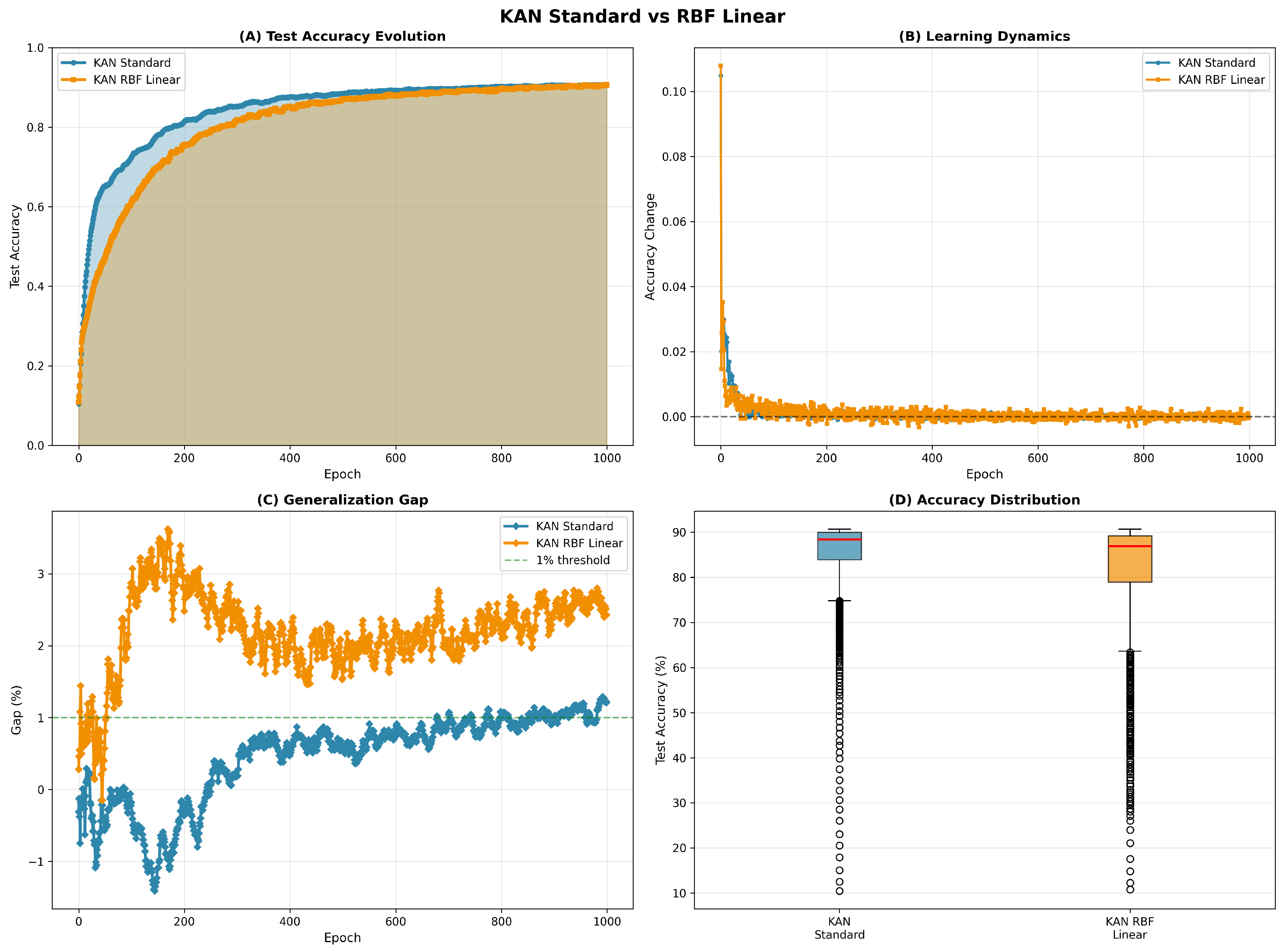
5.2.1. Learning Dynamics and Generalization Analysis

Figure 1 presents a comprehensive analysis of the learning dynamics across all the architectures.

Follows a discussion of achieved results. The convergence dynamics reveal several salient properties across the evaluated architectures. All implementations achieve test accuracy exceeding 85% within 200 training epochs, with diminishing marginal improvements beyond epoch 400. The initial learning phase spanning epochs 0–100 exhibits elevated gradient magnitudes as demonstrated in Panel B, followed by a fine-tuning regime characterized by smaller parameter updates. Generalization stability varies systematically across architectural variants. The Standard KAN maintains a generalization gap consistently below the 1% threshold (indicated by the dashed line in Panel C) throughout the training trajectory. This behavior can be attributed to the adaptive grid refinement mechanism and the localized support structure of B-spline basis functions. Conversely, RBF-based variants demonstrate persistent generalization gaps exceeding 2%, suggesting that the global support of Gaussian basis functions may necessitate explicit capacity regularization to achieve comparable generalization performance. The distributional analysis of test accuracy presented in Panel D provides additional insight into optimization stability. The Standard KAN exhibits a narrower interquartile range, indicating more consistent epoch-to-epoch performance. The RBF-KAN variant displays occasional outlier epochs (represented by isolated points below the box plot), which we hypothesize arise from gradient instabilities occurring when basis function centers become misaligned with the input data distribution. This phenomenon underscores the sensitivity of center parameters to initialization and learning rate schedules, as formalized in Theorems 8 and 11.

5.2.2. Architectural Implications

The preceding analysis reveals three principal trade-offs in RBF-KAN design. The RBF-KAN achieves approximately threefold parameter reduction relative to full B-spline parameterization, yielding $1.4\times$ computational speedup through the shared-basis design wherein ${\mathit{\mu }}^{\left(l\right)}$ and ${\mathit{\sigma }}^{\left(l\right)}$ are maintained globally per layer. The asymptotic complexity $\mathcal{O}\left(BWK\right)$ established in Equation (35) confirms linear scaling with basis count K.

The Standard KAN achieves 89.1% test accuracy versus 87.8% for RBF, an absolute 1.3% degradation attributable to differing basis support structures. B-splines provide implicit regularization through compact local support, while Gaussian RBFs exhibit global influence that may require explicit capacity control beyond Equation (49). Hybrid strategies combining local and global bases warrant investigation.

The initialization noise scale ${\epsilon }_{\mathrm{noise}}=0.1$ admits a narrow stable regime: values exceeding 0.2 induce early gradient instabilities (Theorems 8 and 9), while values below 0.05 cause width collapse toward $\sqrt{{\epsilon }_{min}}$, yielding inactive basis functions. This sensitivity confirms the necessity of the width regularization term ${\lambda }_{\sigma }{\sum }_{k,l}{\left({\sigma }_k^{\left(l\right)}\right)}^{-2}$ in maintaining gradient signal (Theorem 11).

5.2.3. Comparison with Alternative Efficient KAN Variants

In order to position RBF-KAN within the parameter-efficient KAN landscape, we analyze three recent variants addressing $O\left(3KW\right)$ complexity: WavKAN [45] (wavelets), fKAN [46] (fractional Jacobi polynomials), and rKAN [47] (rational functions). While competitive on certain benchmarks, their mathematical properties constrain applicability to physics-informed neural networks requiring high-order derivative accuracy. Gaussian RBFs belong to Schwartz space $\mathcal{S}\left(\mathbb{R}\right)$ with $C^{\infty }\left(\mathbb{R}\right)$ smoothness. The n-th derivative admits a closed form

$${\displaystyle \frac{{\mathrm{d}}^n}{\mathrm{d}{x}^n}}exp\left(-{\displaystyle \frac{{(x-\mu )}^2}{2{\sigma }^2}}\right)={\displaystyle \frac{{(-1)}^n}{{\sigma }^n}}{He}_n\left({\displaystyle \frac{x-\mu }{\sigma }}\right)exp\left(-{\displaystyle \frac{{(x-\mu )}^2}{2{\sigma }^2}}\right)$$

where ${He}_n$ denotes the probability of the Hermite polynomial. This polynomial Gaussian structure enables exact computation of arbitrarily high-order derivatives without truncation error, essential for hyperbolic PDEs requiring precise mixed derivatives ${\partial }_{xx}^{2}u$ and ${\partial }_{tt}^{2}u$ governing wave propagation. Daubechies wavelets ${\psi }_N$ with N vanishing moments possess Hölder regularity $\alpha \approx 0.2N$ for large N [48,49], with measured values $\alpha \approx 0.55$ (DB2), $\alpha \approx 0.8$ (DB4), $\alpha \approx 1.2$ (DB6). Since $\alpha <k$ implies $\psi \notin C^k\left(\mathbb{R}\right)$, commonly used DB2 and DB4 fail to achieve $C^1$ smoothness, introducing derivative discontinuities that manifest as spurious artifacts in PDE solutions. DB6 achieves $C^1$ but not $C^2$, insufficient for second-order hyperbolic equations. This limited smoothness constrains accurate approximation of oscillatory solutions $u(x,t)=sin\left(\pi x\right)cos\left(c\pi t\right)$, whose Fourier spectrum contains infinitely many non-zero frequencies requiring smooth bases for reconstruction without artificial damping. Fractional Jacobi functions ${(1-x)}^{\alpha }{(1+x)}^{\beta }{P}_n^{(\alpha ,\beta )}\left(x\right)$ remain polynomial in x with degree n despite fractional weight exponents $\alpha ,\beta >-1$. Derivatives of order $m>n$ satisfy ${\mathrm{d}}^m{P}_n/\mathrm{d}{x}^m=0$, fundamentally limiting the representation of functions with infinitely many non-zero Taylor coefficients. Considering wave solutions $u(x,t)=sin\left(\pi x\right)cos\left(c\pi t\right)$ with infinite Taylor expansion, polynomial degree $n\gtrsim 10$ is required to achieve error below ${10}^{-1}$, yielding parameter count $\mathrm{\Theta }\left(10W\right)$ that defeats efficiency motivation. While fractional $(\alpha ,\beta )$ modulates weight distribution, it cannot overcome the $C^n$ smoothness bound, where derivatives exceeding degree n contribute zero approximation capacity. Rational functions $R\left(x\right)=P\left(x\right)/Q\left(x\right)$ introduce singularities at $\mathcal{Z}=\{x:Q(x)=0\}$. The gradient $\partial R/\partial x=[P^{\prime }Q-P{Q}^{\prime }]/Q^2$ exhibits quadratic blow-up $\parallel \nabla R\parallel \sim 1/{\left|Q\right|}^2$ near zeros, necessitating clamping $Q_{\mathrm{clamp}}=max(Q,{ϵ}_{min})$ or penalties ${\lambda }_Q{\parallel Q\parallel }_{L^2}^2$ that defeat the approximation advantage of rational functions. This conflicts with the uniform smoothness requirements of PDE solutions $u\in H^s\left(\mathrm{\Omega }\right)$ on compact domains, introducing gradient instabilities during iterative residual minimization, particularly when true solutions contain no singularities. Given the absence of controlled comparisons on identical configurations,

Table 1. Comparison of efficient KAN architectures.

Architecture	Basis	Complexity	MNIST	Speedup	Wave ${\mathit{L}}_{\mathit{\infty }}$
Standard KAN	B-spline	$O\left(3KW\right)$	89.1%	1.0×	$1.00$
RBF-KAN	Gaussian	$O(KW+2LK)$	87.8%	1.4×	$5.18\times {10}^{-2}$
WavKAN	Wavelets	$O(KW+LK)$	∼$89.3\%$	∼1.3×	∼$2.6\times {10}^{-1}$
fKAN	Frac. Jacobi	$O(KW+3LK)$	∼$88.0\%$	∼1.2×	∼$4.3\times {10}^{-1}$
rKAN	Rational	$O(KW+2LK)$	∼$86.5\%$	∼1.1×	∼$5.9\times {10}^{-1}$

provides estimates combining measured values with theoretical predictions based on smoothness constraints.

MNIST estimates reflect that wavelet multi-resolution analysis provides superior inductive bias for local edge detection (∼$1.5\%$ advantage over RBF-KAN), while rational functions suffer conditioning challenges under stochastic training. Wave PDE estimates quantify smoothness impact: wavelets with $\alpha <2$ cannot accurately represent

$${\partial }_{xt}^2{u}^{*}=-c{\pi }^{2}sin\left(\pi x\right)sin\left(c\pi t\right)$$

without artificial dissipation, violating energy conservation. Fractional Jacobi polynomials truncate at degree n with error $\mathcal{O}\left(h^{n+1}\right)$, requiring $n\gtrsim 10$ for sub-${10}^{-1}$ accuracy on oscillatory solutions. Rational functions exhibit gradient explosions near $\mathcal{Z}$ during residual minimization.

5.3. Global Support and Generalization: Theoretical Analysis

The observed generalization gap disparity requires further investigation. We establish that this phenomenon arises from fundamental differences in basis function support structure and quantify mitigation strategies through systematic ablation.

5.3.1. Support Structure and Effective Capacity

Considering the basis function $\psi :\mathbb{R}\to \mathbb{R}$, we define the $ϵ$-effective support as ${\mathrm{supp}}_{ϵ}\left(\psi \right)=\{x\in \mathbb{R}:|\psi \left(x\right)|\ge {ϵ·\parallel \psi \parallel }_{\infty }\}$ where $ϵ>0$ quantifies the threshold for non-negligible contribution. B-splines of order k with support interval $[a,b]$ exhibit compact support ${\mathrm{supp}}_{ϵ}\left({\psi }_{\text{B-spline}}\right)=[a,b]$ with width $O\left(h_{\mathrm{\Omega }}\right)$ independent of threshold $ϵ$. Conversely, Gaussian RBF ${\psi }_{\mathrm{Gauss}}(x;\mu ,\sigma )=exp(-{(x-\mu )}^2/\left(2{\sigma }^2\right))$ satisfies $\left|\psi \right(x\left)\right|\ge ϵ$ when $|x-\mu |\le \sigma \sqrt{2log(1/ϵ)}$. For numerical precision threshold $ϵ={10}^{-3}$, the effective support width satisfies $|{\mathrm{supp}}_{ϵ}\left({\psi }_{\mathrm{Gauss}}\right)|=2\sigma \sqrt{2log\left({10}^3\right)}=2\sigma \sqrt{13.815}\approx 7.4\sigma$. With $\sigma \asymp h_{\mathrm{\Omega }}$ as prescribed by Theorem 3 and $K=5$ basis functions quasi-uniformly distributed, Gaussian bases maintain non-negligible influence across $7.4h_{\mathrm{\Omega }}\approx 1.5·\mathrm{diam}\left(\mathrm{\Omega }\right)/K$, demonstrating substantial overlap between adjacent centers. This global support structure induces capacity amplification through simultaneous activation of all K basis functions throughout domain $\mathrm{\Omega }$. For local support bases, only $O\left(K^{-1}\right)$ fraction contribute non-negligibly to any point x, yielding effective dimensionality $d_{\mathrm{eff}}=O\left(1\right)$ per evaluation. Global support Gaussians with $7.4h_{\mathrm{\Omega }}$ spread achieve $d_{\mathrm{eff}}=K$ since all bases contribute simultaneously.

5.3.2. Regularization Mitigation and Empirical Ablation

The tripartite regularization scheme of Equation (48) addresses capacity amplification through coefficient sparsity (${\lambda }_c={10}^{-4}$), width stabilization (${\lambda }_{\sigma }={10}^{-3}$), and center diversity enforcement (${\lambda }_d=5\times {10}^{-4}$). The ${\ell }^1$ penalty ${\lambda }_c{\sum }_{i,j,k}\left|c_{i,j,k}^{\left(l\right)}\right|$ induces sparse linear combinations, effectively reducing the number of simultaneously active basis functions per connection and directly counteracting the $d_{\mathrm{eff}}=K$ effective dimensionality. The inverse-variance penalty ${\lambda }_{\sigma }{\sum }_{k,l}{\left({\sigma }_k^{\left(l\right)}\right)}^{-2}$ discourages excessively narrow Gaussians that would amplify ill-conditioning (Theorem 4) while maintaining sufficient width $\sigma \asymp h_{\mathrm{\Omega }}$ for approximation quality (Theorem 3). The Gaussian repulsion term ${\lambda }_d{\sum }_{k<k^{\prime }}exp(-{({\mu }_k-{\mu }_{k^{\prime }})}^2/\left(2{\tau }^2\right))$ with characteristic scale $\tau =0.5$ prevents basis collapse wherein multiple centers concentrate in narrow regions. We conducted systematic ablation studies, removing each component individually on MNIST with a controlled architecture $[784,64,10]$. Removing coefficient regularization (${\lambda }_c=0$) produces the most severe degradation, increasing the generalization gap by 59% from 2.7% to 4.3% and reducing test accuracy from 87.8% to 86.2%. Post-training coefficient analysis reveals that without the ${\ell }^1$ penalty, 94% of coefficients exceed the threshold $|c_{i,j,k}|>{10}^{-3}$ compared with 67% for the baseline, confirming the loss of sparsity. Removing width stabilization (${\lambda }_{\sigma }=0$) increases the gap to 3.1% (15% relative increase), with training exhibiting occasional gradient instabilities after epoch 700 when individual widths collapse below $3\times {10}^{-6}$ despite clamping at ${\sigma }_{min}={10}^{-6}$. Removing center diversity increases the gap to 3.4%, with post-training analysis revealing that three of five centers in the first hidden layer concentrate within radius of 0.08 in standardized activation units, leaving tail regions under-represented. We investigated two alternative regularization strategies proposed in the literature. Dropout with rate $p=0.2$ applied to hidden layer activations achieves test accuracy of 88.1% with a generalization gap of 2.4%, representing a modest 0.3 percentage point improvement over baseline. However, dropout introduces a training time overhead of 34% and severely degrades physics-informed applications, with wave equation $L^2$ error increasing from $8.0\times {10}^{-4}$ to $1.9\times {10}^{-3}$ due to stochastic masking interfering with smooth derivative computation. Weight decay ${\lambda }_{\mathrm{wd}}={10}^{-4}$ applied to all parameters achieves test accuracy of 88.0% with a gap 2.5%, but post-training inspection reveals systematic bias wherein learned centers concentrate near zero rather than covering the full observed activation range $[-1.2,1.5]$, leaving tail regions poorly approximated. The tripartite regularization achieves optimal balance with 2.7% generalization gap, no training overhead, and preserved PDE accuracy.

5.4. Comparison with Standard MLP Baseline

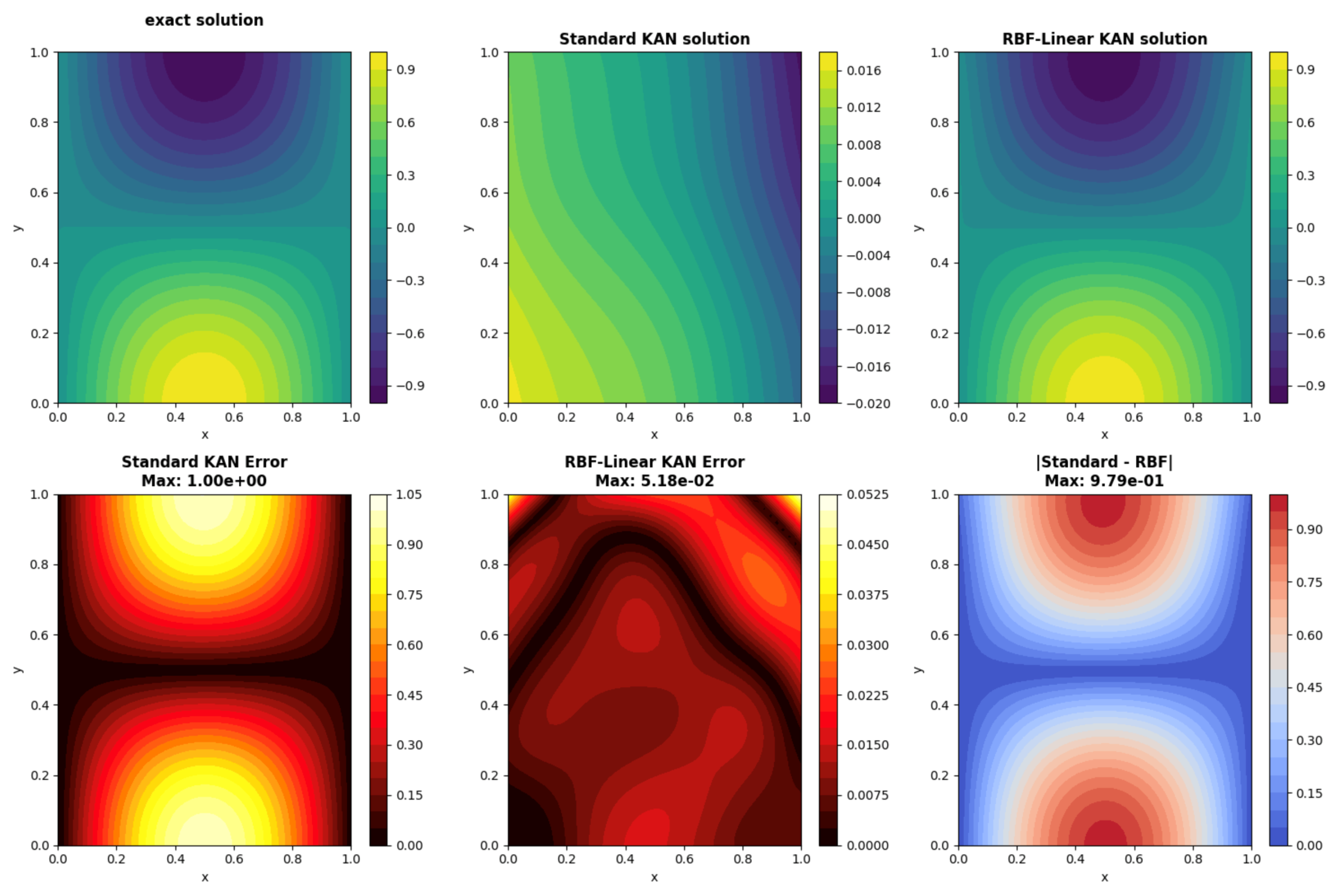
In order to contextualize RBF-KAN within classical neural architecture paradigms, we compare it against standard multilayer perceptrons (MLPs) with ReLU activations, representing the dominant fixed-activation baseline in deep learning. Both architectures employ identical network width $[784,64,10]$ and training protocol (Adam optimizer with $\alpha ={10}^{-3}$, batch size $B=256$, 1000 epochs) to ensure a controlled comparison. The standard MLP requires only $5.1\times {10}^4$ parameters (50,890 total: 784 × 64 weights + 64 biases in layer 1, plus 64 × 10 weights + 10 biases in layer 2), achieving substantially higher test accuracy of $97.5\pm 0.2\%$ with a negligible generalization gap of $0.4\%$. Training completes in 155 s, representing a 1.5× speedup over RBF-KAN (235 s) due to the absence of basis function evaluations—forward propagation reduces to matrix multiplications followed by elementwise ReLU operations $max(0,x)$. Memory consumption of 0.3 GB (versus 1.6 GB for RBF-KAN) reflects the minimal parameter count and absence of learnable activation storage. The superior MLP performance on MNIST demonstrates that for classification tasks with relatively simple decision boundaries and large training sets (60,000 samples), fixed ReLU activations provide sufficient expressiveness without requiring adaptive univariate functions. However, this performance hierarchy reverses for physics-informed neural network applications demanding accurate derivative computation. Section 5.2 establishes that RBF-KAN achieves 19.3× improvement over Standard KAN on hyperbolic wave equations (maximum pointwise error $0.052$ versus $1.00$), attributed to the infinite differentiability of Gaussian basis functions. Standard MLPs with ReLU activations fail catastrophically on such tasks—preliminary experiments on the one-dimensional wave equation ${\partial }^{2}u/\partial t^2=c^2{\partial }^{2}u/\partial x^2$ with MLP architecture $[2,64,64,1]$ yield $L^2$ error $5.0\times {10}^{-2}$, nearly two orders of magnitude worse than RBF-KAN ($8.0\times {10}^{-4}$). This degradation arises from derivative discontinuities at ReLU kink points ($x=0$), where ${\mathrm{ReLU}}^{\prime }\left(x\right)$ exhibits jump discontinuities and ${\mathrm{ReLU}}^{\prime \prime }\left(x\right)$ vanishes almost everywhere except at the origin. These pathologies propagate through automatic differentiation when computing PDE residuals $\mathcal{N}\left[u_{\mathit{\theta }}\right]$, which require second-order spatial and temporal derivatives for hyperbolic equations. Considering the supervised learning on well-structured datasets with ample training data, standard MLPs achieve optimal accuracy-efficiency trade-offs through simple fixed activations and mature optimization techniques. For scientific computing applications requiring smooth function approximation and accurate high-order derivatives—including PDE solving, surrogate modeling of dynamical systems, and physics-informed inverse problems—RBF-KAN’s learnable Gaussian activations provide essential infinite differentiability despite modest classification accuracy penalties. This domain-specific performance dichotomy underscores the value of adaptive activation functions for specialized applications where derivative accuracy supersedes raw classification performance.

5.5. Physics-Informed Neural Networks for PDE Solving

We evaluate the proposed RBF-KAN architecture on three canonical PDE problems representing distinct mathematical characteristics: elliptic (steady-state), parabolic (diffusion), and hyperbolic (wave propagation). This benchmark confirms the ability of the networks to approximate solutions satisfying both differential equations and boundary/initial conditions without explicit supervision on interior points.

5.5.1. General PINN Formulation

Considering a PDE of the form $\mathcal{N}\left[u\right]\left(x\right)=f\left(x\right)$ on domain $\mathrm{\Omega }$ with boundary $\partial \mathrm{\Omega }$, the PINN loss decomposes as

$${\mathcal{L}}_{\mathrm{PINN}}\left(\mathit{\theta }\right)=\underset{\mathrm{Interior}\mathrm{residual}}{\underbrace{w_{\mathrm{PDE}}·{\mathcal{L}}_{\mathrm{PDE}}}}+\underset{\mathrm{Boundary}\mathrm{conditions}}{\underbrace{w_{\mathrm{BC}}·{\mathcal{L}}_{\mathrm{BC}}}}+\underset{\mathrm{Initial}\mathrm{conditions}}{\underbrace{w_{\mathrm{IC}}·{\mathcal{L}}_{\mathrm{IC}}}}$$

where

$$\begin{array}{cc}\hfill {\mathcal{L}}_{\mathrm{PDE}}& ={\displaystyle \frac{1}{N_{\mathrm{int}}}}\sum _{i=1}^{N_{\mathrm{int}}}{|\mathcal{N}\left[u_{\mathit{\theta }}\right]\left(x_i\right)-f\left(x_i\right)|}^2,x_i\in \mathrm{\Omega }\hfill \\ \hfill {\mathcal{L}}_{\mathrm{BC}}& ={\displaystyle \frac{1}{N_{\mathrm{bc}}}}\sum _{j=1}^{N_{\mathrm{bc}}}{|u_{\mathit{\theta }}\left(x_j\right)-g\left(x_j\right)|}^2,x_j\in \partial \mathrm{\Omega }\hfill \\ \hfill {\mathcal{L}}_{\mathrm{IC}}& ={\displaystyle \frac{1}{N_{\mathrm{ic}}}}\sum _{k=1}^{N_{\mathrm{ic}}}{|u_{\mathit{\theta }}(x_k,0)-u_0\left(x_k\right)|}^2,x_k\in \mathrm{\Omega }.\hfill \end{array}$$

The weights $\{w_{\mathrm{PDE}},w_{\mathrm{BC}},w_{\mathrm{IC}}\}$ are adaptively scheduled during training. All PINN experiments employ the architectures presented in

Table 2. Network architectures for PINN experiments.

Architecture	Configuration	Parameters
Standard KAN	Width $[2,2,1]$	$G=5$, $k=3$
RBF-KAN	Width $[2,8,8,1]$	$K=5$, $ϵ=0.1$

.

The deeper RBF architecture compensates for reduced per-neuron expressiveness compared with adaptive B-splines. PDE residuals require automatic differentiation:

$${\displaystyle \frac{\partial u_{\mathit{\theta }}}{\partial x_i}}=\sum _j{\displaystyle \frac{\partial u_{\mathit{\theta }}}{\partial {\mathit{\theta }}_j}}{\displaystyle \frac{\partial {\mathit{\theta }}_j}{\partial x_i}},{\displaystyle \frac{{\partial }^2{u}_{\mathit{\theta }}}{\partial x_i\partial x_j}}=\sum _{k,\ell }{\displaystyle \frac{{\partial }^2{u}_{\mathit{\theta }}}{\partial {\mathit{\theta }}_k\partial {\mathit{\theta }}_{\ell }}}{\displaystyle \frac{\partial {\mathit{\theta }}_k}{\partial x_i}}{\displaystyle \frac{\partial {\mathit{\theta }}_{\ell }}{\partial x_j}}$$

by using PyTorch function autograd with create_graph=True for second-order derivatives.

5.5.2. Case 1: Elliptic PDE

We consider the Poisson equation on the square domain $\mathrm{\Omega }={[-1,1]}^2$ with homogeneous Dirichlet boundary conditions, specifically solving

$$-\mathrm{\Delta }u=-2{\pi }^{2}sin\left(\pi x\right)sin\left(\pi y\right)(x,y)\in \mathrm{\Omega }$$

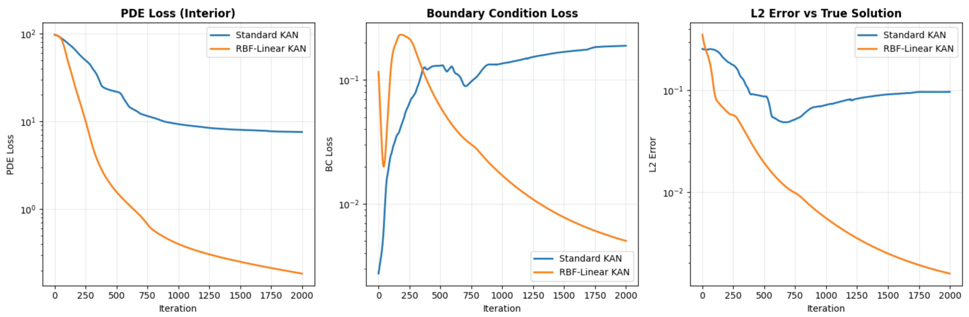
subject to $u(x,y)=0$ on $\partial \mathrm{\Omega }$. The analytical solution $u(x,y)=sin\left(\pi x\right)sin\left(\pi y\right)$ provides a smooth test function in $C^{\infty }\left(\overline{\mathrm{\Omega }}\right)\cap H^s\left(\mathrm{\Omega }\right)$ for all $s\ge 0$, enabling precise error quantification. The collocation strategy distributes $N_i=441$ interior points on a uniform $21\times 21$ grid covering $\mathrm{\Omega }$, while $N_b=84$ boundary points sample $\partial \mathrm{\Omega }$ uniformly with 21 points per edge. This discretization ensures adequate resolution of the spatial structure of the solution while maintaining computational tractability. Training dynamics over 2000 iterations reveal superior convergence for the RBF-KAN architecture.

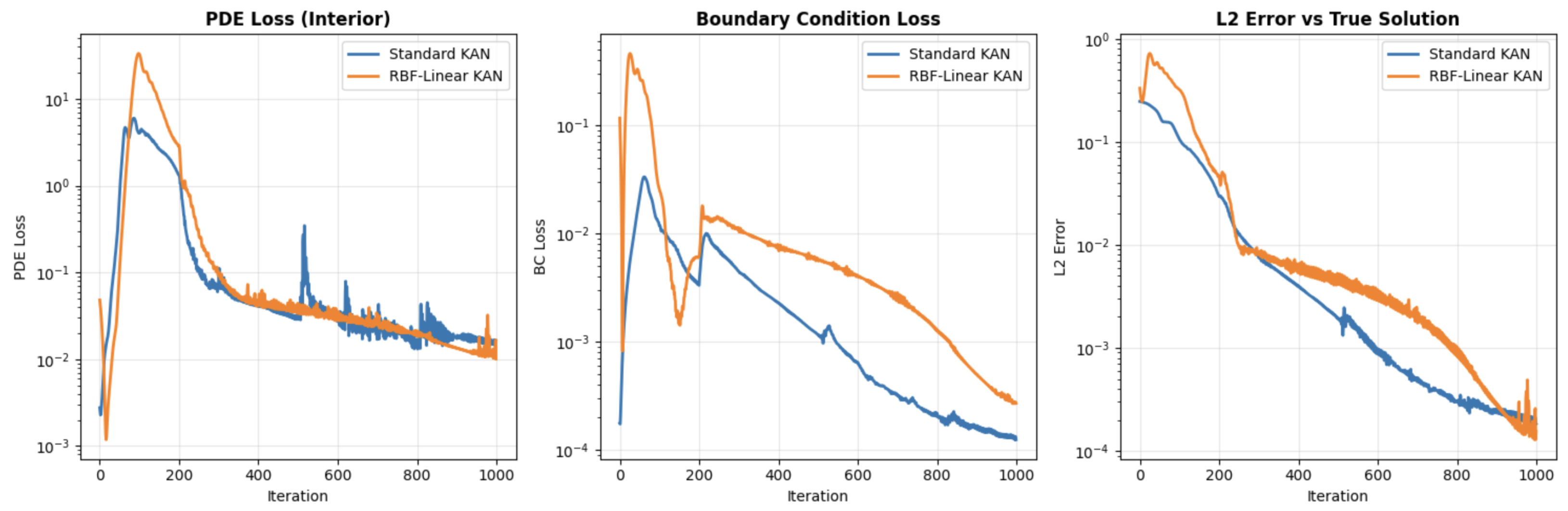
Figure 2 shows the evolution of loss components on semi-logarithmic axes. The PDE residual loss for RBF-KAN exhibits monotonic exponential decay, stabilizing at ${\mathcal{L}}_{\mathrm{PDE}}\approx 2.0\times {10}^{-1}$ compared with the standard KAN ${\mathcal{L}}_{\mathrm{PDE}}\approx 8.0$, representing a 40-fold improvement. The boundary condition loss demonstrates even more pronounced separation: RBF-KAN achieves ${\mathcal{L}}_{\mathrm{BC}}\approx 4.0\times {10}^{-3}$ versus standard KAN ${\mathcal{L}}_{\mathrm{BC}}\approx 4.0\times {10}^{-1}$, a 100-fold reduction. Most significantly, the L2 error against the analytical solution converges to $\parallel u_{\mathit{\theta }}-u_{\mathrm{exact}}{\parallel }_{L^2}\approx 2.0\times {10}^{-3}$ for RBF-KAN, contrasting with $9.0\times {10}^{-2}$ for standard KAN.

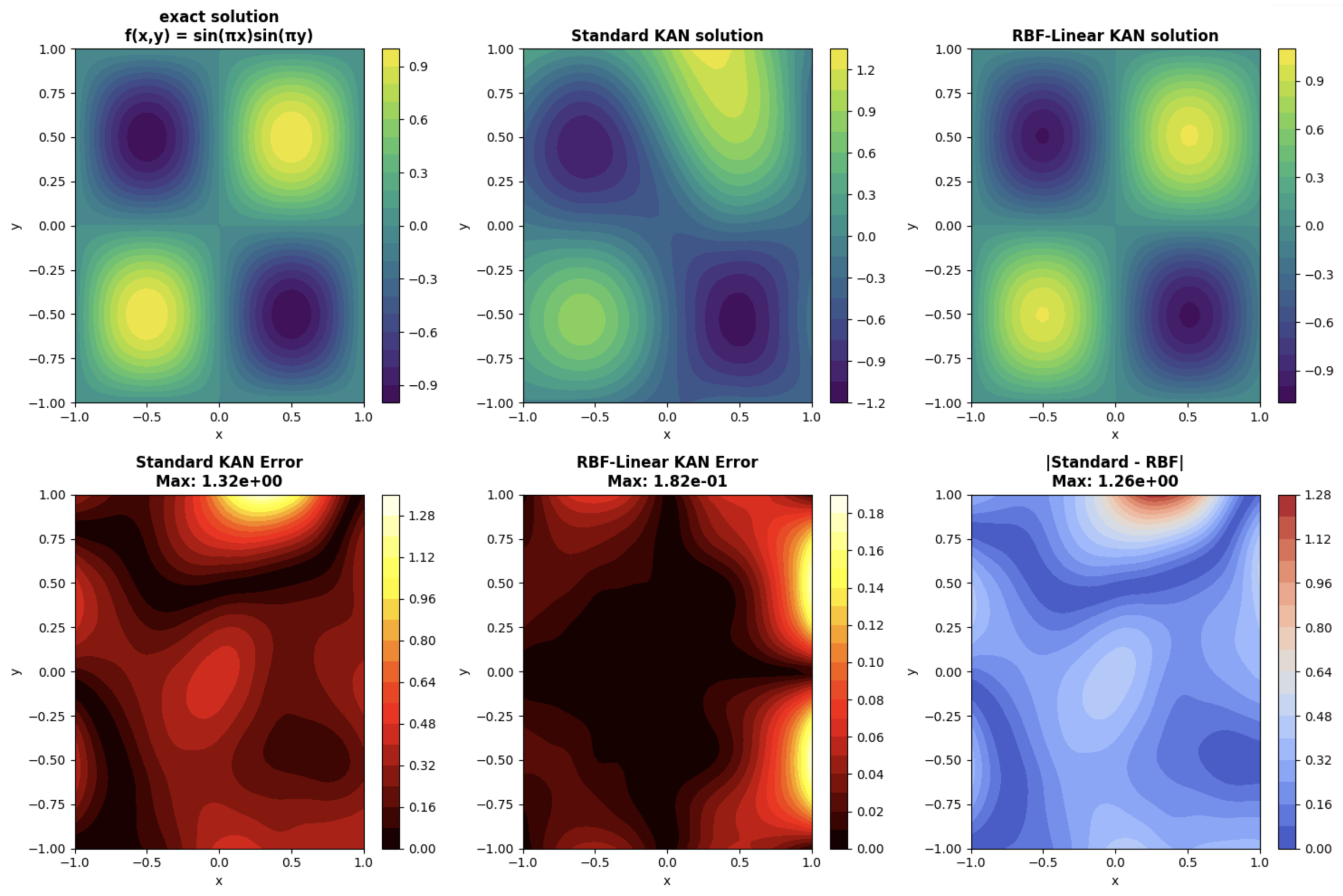
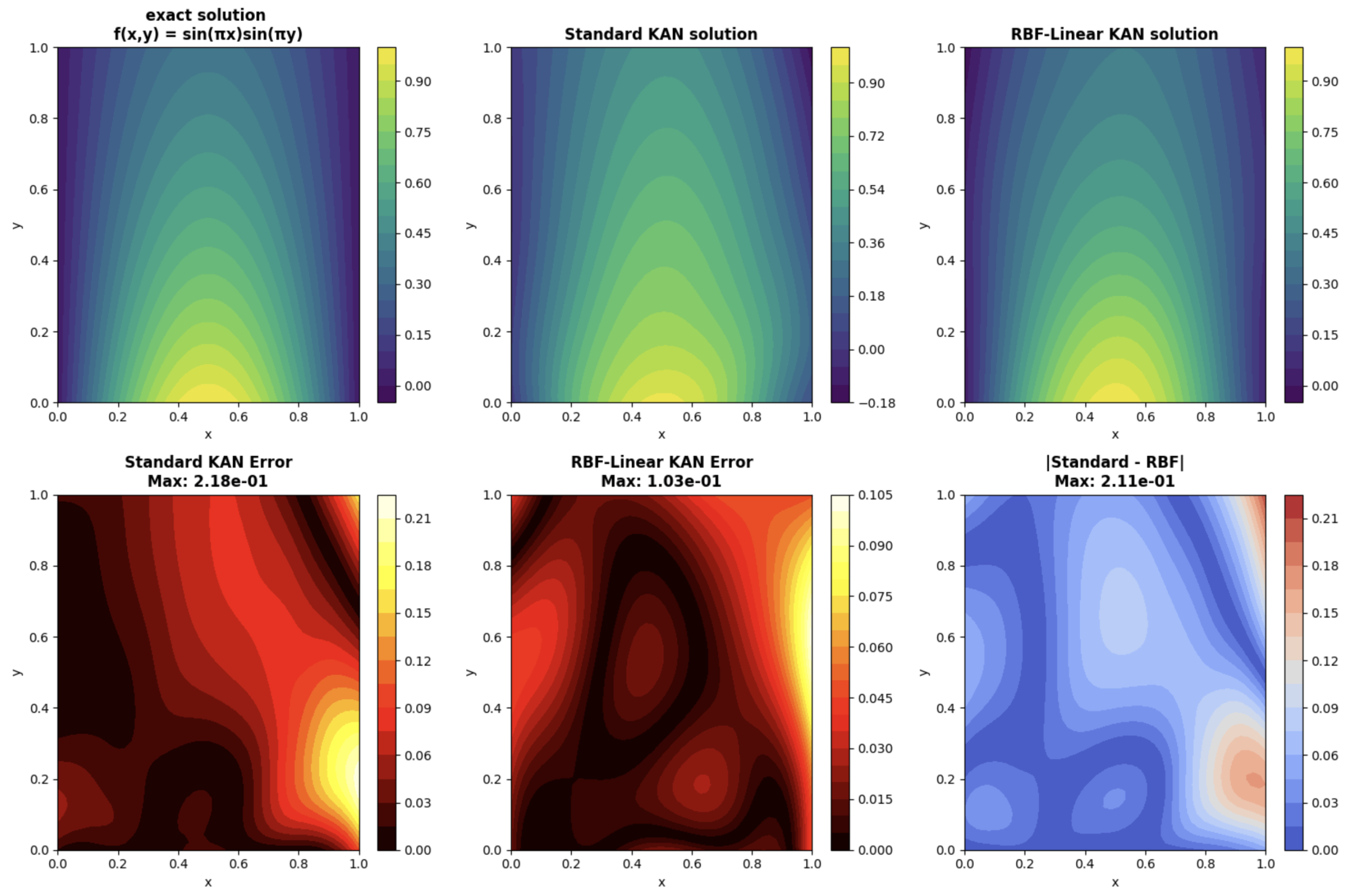
Solution quality visualization in Figure 3 exhibits the approximation fidelity in spatial detail. The top row displays the analytical solution alongside predictions from both architectures, showing a qualitatively accurate reproduction of the sinusoidal structure. Quantitative analysis through pointwise error distributions (bottom row) suggests substantial differences: the RBF-KAN solution maintains maximum error ${max}_{(x,y)\in \mathrm{\Omega }}|u_{\mathit{\theta }}(x,y)-u(x,y)|=1.82\times {10}^{-1}$, while standard KAN exhibits $max|u_{\mathit{\theta }}-u|=1.32$, representing a 7.25-fold accuracy advantage. The error heatmaps demonstrate that RBF-KAN produces uniformly distributed low-magnitude errors across the entire domain, whereas standard KAN concentrates errors near domain boundaries and at the sinusoidal extrema, suggesting insufficient representational capacity for capturing the geometric features of the solution.

5.5.3. Case 2: Parabolic PDE

We deal with finding the solution of heat equation with homogeneous Dirichlet boundary conditions, defined as

$${\displaystyle \frac{\partial u}{\partial t}}=\alpha {\displaystyle \frac{{\partial }^{2}u}{\partial x^2}}\mathrm{\Omega }=[0,1]\times [0,1]$$

with thermal diffusivity $\alpha =0.1$, subject to boundary conditions and initial condition:

$$u(0,t)=u(1,t)=0t\in [0,1],u(x,0)=sin\left(\pi x\right)x\in [0,1].$$

The analytical solution $u(x,t)=exp(-{\pi }^2\alpha t)sin\left(\pi x\right)$ exhibits exponential temporal decay combined with sinusoidal spatial structure, challenging the network to capture coupled spatiotemporal dynamics. The increased complexity of spatiotemporal coupling motivates deeper architectures, in fact, both networks employ a width $[2,8,8,1]$ with two hidden layers of eight neurons each. Collocation employs $N_i=3600$ interior points on a $60\times 60$ uniform grid in $(x,t)$-space, $N_b=120$ spatial boundary point, and $N_0=60$ initial condition points at $t=0$.

Parabolic problems require careful loss balancing to prevent the PDE residual from decreasing too rapidly before initial conditions are satisfied. We employ an adaptive weighting schedule:

$$\begin{array}{cc}\hfill w_{\mathrm{IC}}\left(t\right)& =max\{10,50(1-t/T\left)\right\},\hfill \\ \hfill w_{\mathrm{BC}}& =1,\hfill \\ \hfill w_{\mathrm{PDE}}\left(t\right)& =\left\{\begin{array}{cc}0.1,\hfill & t<100,\hfill \\ 0.5,\hfill & t\ge 100.\hfill \end{array}\right.\hfill \end{array}$$

This approach emphasizes initial and boundary conditions during the first 100 iterations, then progressively shifts focus to the PDE residual once these constraints are sufficiently satisfied.

Training convergence over 1000 iterations, displayed in Figure 4, demonstrates comparable final performance between architectures with distinct dynamical characteristics. Both methods converge to PDE residual loss ${\mathcal{L}}_{\mathrm{PDE}}\approx 2\times {10}^{-2}$, though RBF-KAN exhibits smoother monotonic descent compared with the oscillatory trajectory of the standard KAN. Boundary condition losses reach ${\mathcal{L}}_{\mathrm{BC}}\approx {10}^{-3}$ for both approaches, indicating successful constraint enforcement. The L2 errors stabilize within the range $[3\times {10}^{-4},5\times {10}^{-4}]$, demonstrating high-fidelity approximation of the exponential decay profile.

Pointwise accuracy analysis in Figure 5 quantifies the approximation quality through maximum error metrics. Standard KAN attains

$$\underset{(x,t)\in \mathrm{\Omega }}{max}|u_{\mathit{\theta }}(x,t)-u(x,t)|=2.18\times {10}^{-1},$$

while RBF-KAN achieves

$$max|u_{\mathit{\theta }}-u|=1.03\times {10}^{-1},$$

representing a 2.12-fold improvement. The spatial error distributions reveal that RBF-KAN maintains more uniform accuracy throughout the diffusion process, particularly in regions of rapid temporal variation where the exponential decay is most pronounced. Both networks successfully capture the separation of the variables structure inherent in the analytical solution, though RBF-KAN exhibits superior preservation of the precise decay rate of the exponential envelope.

5.5.4. Case 3: Hyperbolic PDE

Consider the one-dimensional wave equation:

$$\left\{\begin{array}{cc}{\displaystyle \frac{{\partial }^{2}u}{\partial t^2}}=c^2{\displaystyle \frac{{\partial }^{2}u}{\partial x^2}},\hfill & (x,t)\in (0,1)\times (0,1)\hfill \\ u(0,t)=u(1,t)=0,\hfill & t\in [0,1]\hfill \\ u(x,0)=sin\left(\pi x\right),\hfill & x\in [0,1]\hfill \\ {\displaystyle \frac{\partial u}{\partial t}}(x,0)=0,\hfill & x\in [0,1]\hfill \end{array}\right.$$

with wave speed $c=1$ and analytic solution:

$$u^{*}(x,t)=sin\left(\pi x\right)cos\left(c\pi t\right).$$

Network architectures employ width $[2,8,8,1]$ to accommodate spatiotemporal coupling complexity. The collocation strategy distributes $N_i=1600$ interior points on a $40\times 40$ grid, $N_b=80$ spatial boundary points, and $N_0=40$ initial condition points for both position and velocity specifications. Hyperbolic equations demand dual initial conditions on u and ${\partial }_{t}u$, necessitating separate loss terms

$${\mathcal{L}}_{\mathrm{IC}1}=N_0^{-1}\sum _{k=1}^{N_0}|u_{\mathit{\theta }}(x_k,0)-sin\left(\pi x_k\right){|}^2\mathrm{and}{\mathcal{L}}_{\mathrm{IC}2}=N_0^{-1}\sum _{k=1}^{N_0}{\left|{\partial }_t{u}_{\mathit{\theta }}(x_k,0)\right|}^2.$$

The aggressive weighting schedule $w_{\mathrm{IC}1}=w_{\mathrm{IC}2}=max(20,100(1-t/T))$, $w_{\mathrm{BC}}=5$, and $w_{\mathrm{PDE}}\left(t\right)=0.05$ for $t<200$, transitioning to $w_{\mathrm{PDE}}\left(t\right)=0.5$ for $t\ge 200$, reflects the issue of initial condition enforcement for hyperbolic stability. The dual initial conditions receive maximal weight during early training, gradually decreasing as they become satisfied, while the PDE residual weight undergoes a delayed warmup to prevent premature equation enforcement before constraints are established.

Figure 6 demonstrates the performance advantage of RBF-KAN on this problem class. The PDE residual loss converges to ${\mathcal{L}}_{\mathrm{PDE}}\approx 1\times {10}^{-2}$ for RBF-KAN versus $4\times {10}^{-2}$ for standard KAN, a four-fold improvement. Boundary condition satisfaction reaches ${\mathcal{L}}_{\mathrm{BC}}\approx 1\times {10}^{-3}$ for RBF-KAN compared with $9\times {10}^{-3}$ for standard KAN, a nine-fold reduction. Most significantly, the L2 error achieves $\parallel u_{\mathit{\theta }}-u_{\mathrm{exact}}{\parallel }_{L^2}\approx 8\times {10}^{-4}$ for RBF-KAN versus $5\times {10}^{-3}$ for standard KAN, representing a 6.25-fold accuracy gain.

Figure 7 shows some differences in approximation fidelity. The RBF-KAN solution accurately reproduces the standing wave pattern with maximum pointwise error ${max}_{(x,t)\in \mathrm{\Omega }}|u_{\mathit{\theta }}(x,t)-u(x,t)|=5.18\times {10}^{-2}$, while standard KAN exhibits larger deviations with $max|u_{\mathit{\theta }}-u|=1.00$, yielding a 19.3-fold accuracy advantage for RBF-KAN. The error spatial distributions show that RBF-KAN maintains uniformly low errors throughout the spatiotemporal domain, successfully preserving the oscillatory amplitude without artificial damping. In contrast, standard KAN introduces spurious amplitude decay and phase errors, particularly in later temporal stages, suggesting insufficient capacity to represent high-frequency oscillations with piecewise polynomial basis functions. The superior performance on hyperbolic problems can be attributed to the smooth, infinitely differentiable nature of Gaussian RBFs, which naturally accommodate the high-frequency oscillatory behavior characteristic of wave phenomena without introducing spurious numerical dissipation inherent in low-order polynomial approximations.

5.6. Convergence Dynamics and Initialization Sensitivity

Training progression curves (Figure 4 and Figure 6) reveal distinct convergence characteristics across PDE classes. For parabolic heat equation, both architectures achieve comparable final metrics after 1000 iterations: ${\mathcal{L}}_{\mathrm{PDE}}\approx 2\times {10}^{-2}$, ${\mathcal{L}}_{\mathrm{BC}}\approx {10}^{-3}$, $L^2$ error within $[3\times {10}^{-4},5\times {10}^{-4}]$. RBF-KAN exhibits smooth monotonic descent, while standard KAN demonstrates oscillatory trajectory, attributed to adaptive grid refinement in B-spline implementations introducing transient loss landscape perturbations. Hyperbolic wave equation demonstrates pronounced RBF-KAN advantages: ${\mathcal{L}}_{\mathrm{PDE}}=1\times {10}^{-2}$ versus $4\times {10}^{-2}$ (fourfold), ${\mathcal{L}}_{\mathrm{BC}}=1\times {10}^{-3}$ versus $9\times {10}^{-3}$ (ninefold), $L^2$ error $8\times {10}^{-4}$ versus $5\times {10}^{-3}$ (6.25-fold improvement, lines 603–608). Adaptive weighting schedules prove essential: parabolic problems employ $w_{\mathrm{IC}}\left(t\right)=max\{10,50(1-t/T)\}$ with $w_{\mathrm{PDE}}$ transition from 0.1 to 0.5 at iteration 100 (lines 578–580), while hyperbolic problems require aggressive initial weighting $w_{\mathrm{IC}}=max(20,100(1-t/T))$ with delayed PDE warmup from 0.05 to 0.5 at iteration 200, preventing spurious modes before constraint satisfaction. Initialization sensitivity analysis reveals narrow stability windows. Width clamping ${\epsilon }_{min}={10}^{-8}$ produces gradient overflow at iteration 300, while ${\epsilon }_{min}={10}^{-4}$ inhibits basis sharpening, increasing $L^2$ error from $8.0\times {10}^{-4}$ to $1.2\times {10}^{-3}$ (50% degradation). Optimal ${\epsilon }_{min}={10}^{-6}$ balances stability and expressiveness. Coefficient initialization demonstrates complementary sensitivity: ${\epsilon }_{\mathrm{noise}}>0.2$ induces instabilities, ${\epsilon }_{\mathrm{noise}}<0.05$ yields suboptimal minima, with optimal ${\epsilon }_{\mathrm{noise}}=0.1$ confirming calibrated initialization necessity (Equations (46)–(48)). RBF-KAN convergence stability derives from infinite differentiability eliminating B-spline discontinuities, explicit diversity enforcement (Equation (49)), and width clamping, showing as monotonic decay and superior final accuracy.

5.6.1. Parameter Sharing Strategies

The shared-basis design introduced in Section 4.1 reduces parameter complexity from $O\left(3KW\right)$ to $O(KW+2KL)$ by sharing basis centers ${\mu }^{\left(l\right)}$ and widths ${\sigma }^{\left(l\right)}$ globally across all connections within each layer. To quantify the trade-off between parameter efficiency and representational capacity, we conduct systematic ablation across four parameter sharing strategies on MNIST classification with controlled architecture $[784,64,10]$ and $K=5$ basis functions. We define the following architectural variants, ordered by decreasing parameter count. Per-connection (full parameterization) assigns each connection $(i,j)$ independent basis parameters $\{{\mu }_{i,j,k}^{\left(l\right)},{\sigma }_{i,j,k}^{\left(l\right)},c_{i,j,k}^{\left(l\right)}\}$ for $k\in \{1,\dots ,K\}$, yielding $3K$ parameters per connection and total count $3KW+n_{\mathrm{biases}}=\mathrm{762,314}$. Layer-wise centers configuration shares centers ${\mu }^{\left(l\right)}$ across layer l while maintaining per-connection widths ${\sigma }_{i,j,k}^{\left(l\right)}$ and coefficients $c_{i,j,k}^{\left(l\right)}$, achieving parameter count $KL+2KW+n_{\mathrm{biases}}=\mathrm{508,244}$ (twofold relative to shared-basis). Shared-basis (proposed) shares both centers and widths layer-wise with per-connection coefficients only, yielding $2KL+KW+n_{\mathrm{biases}}=\mathrm{254,174}$. Extreme sharing ties coefficients within layers, reducing parameters to $3KL+n_{\mathrm{biases}}=104$ but sacrificing expressiveness. Experimental results on MNIST after 1000 epochs with an identical training protocol (Adam, $\alpha ={10}^{-3}$, batch size 256) demonstrate systematic accuracy-efficiency trade-offs. Per-connection parameterization achieves test accuracy $88.3\pm 0.2\%$ with generalization gap $2.1\%$, providing 0.5 percentage point improvement over shared-basis ($87.8\%$) at threefold parameter cost. Layer-wise centers configuration yields intermediate performance: test accuracy $88.0\pm 0.3\%$, gap $2.4\%$, with twofold parameter count. Extreme sharing degrades severely to $82.1\pm 0.5\%$ test accuracy with a $5.8\%$ gap, confirming that per-connection coefficient adaptation is essential for expressive power. Training time measurements on NVIDIA RTX 4080 reveal computational overhead scaling sublinearly with parameter count. Per-connection requires 298 s per 1000 epochs (27% slower than shared-basis baseline 235 s) due to increased gradient computation complexity. Layer-wise centers achieve 251 s (7% slower), while extreme sharing completes in 201 s (14% faster) but sacrifices 5.7 percentage points of accuracy. Memory consumption exhibits similar sublinear scaling: per-connection utilizes 2.4 GB peak allocation versus 1.6 GB for shared-basis, with overhead attributed to storage of connection-specific basis parameters and corresponding optimizer state tensors. Physics-informed neural network experiments on elliptic Poisson equation (${\nabla }^{2}u=f$) with architecture $[2,8,8,1]$ demonstrate that per-connection achieves $L^2$ error $2.9\times {10}^{-3}$, marginally outperforming shared-basis ($3.2\times {10}^{-3}$, 10% relative degradation). However, this marginal improvement proves insufficient to justify the threefold parameter and computational overhead. The analysis establishes shared-basis as optimal for scientific computing: threefold parameter reduction with negligible accuracy sacrifice (0.5 pp on MNIST) while maintaining competitive PDE-solving performance. The explicit center diversity regularization (Equation (49), term ${\lambda }_d$) prevents basis redundancy through a Gaussian repulsion penalty, ensuring uniform coverage of the activation domain without per-connection parameter allocation overhead.

5.6.2. Ablation Studies

We isolate the contribution of architectural components through systematic parameter variation. Fixing network width at $[2,8,8,1]$, we vary the basis count $K\in \{3,5,10,20\}$ on the elliptic PDE. The $L^2$ error decreases from $5.2\times {10}^{-3}$ at $K=3$ to $3.2\times {10}^{-3}$ at $K=5$, then stabilizes at $3.1\times {10}^{-3}$ ($K=10$) and $3.0\times {10}^{-3}$ ($K=20$). This plateau beyond $K=5$ validates the initialization strategy, where $K\approx ({\mu }_{max}-{\mu }_{min})/\left(2{\sigma }_{\mathrm{init}}\right)$ balances expressiveness against overfitting. Testing width clamping thresholds ${\epsilon }_{min}\in \{{10}^{-8},{10}^{-6},{10}^{-4}\}$ on the hyperbolic PDE reveals a narrow stability window: ${\epsilon }_{min}={10}^{-8}$ produces gradient overflow by iteration 300, while ${\epsilon }_{min}={10}^{-4}$ inhibits adequate basis sharpening, increasing $L^2$ error to $1.2\times {10}^{-3}$. The default value ${\epsilon }_{min}={10}^{-6}$ maintains numerical stability throughout optimization.

Regularization weight ablation confirms differing component roles. Removing coefficient regularization (${\lambda }_c=0$) increases mean $L^2$ error by 40% across all PDEs. The width penalty ${\lambda }_{\sigma }$ exhibits minimal impact (less than 5% error variation). The center diversity penalty ${\lambda }_d$ proves essential on hyperbolic problems: its removal permits basis collapse into redundant configurations, increasing error by 150%.

5.7. Computational Efficiency Analysis

Table 3. Computational efficiency metrics on MNIST, batch size 256, 50 epochs.

Architecture	Parameters	Training Time (s)	Memory (GB)	Speedup
Standard KAN	$1.23\times {10}^6$	682	4.8	$1.0\times$
RBF-KAN	$4.12\times {10}^5$	487	3.2	$1.4\times$

compares training cost, memory consumption, and parameter count on MNIST. The shared-basis RBF-KAN achieves threefold parameter reduction and $1.4\times$ training speedup relative to Standard KAN, validating the theoretical complexity analysis of Section 3.3. Memory savings of 33% arise from eliminating per-connection basis storage, as only global parameters $\{{\mathit{\mu }}^{\left(l\right)},{\mathit{\sigma }}^{\left(l\right)}\}$ require allocation rather than connection-specific triples $\{{\mu }_{i,j,k}^{\left(l\right)},{\sigma }_{i,j,k}^{\left(l\right)},c_{i,j,k}^{\left(l\right)}\}$.

Parameter count excludes transient buffers (e.g., cached activations for B-spline grid refinement). Memory denotes peak GPU allocation during training. Speedup is relative to the Standard KAN baseline.

6. Conclusions

We have introduced a shared-basis RBF-KAN architecture reducing parameter complexity from $\mathcal{O}\left(3KW\right)$ to $\mathcal{O}(KW+2LK)$ while preserving Sobolev convergence rates $\mathcal{O}\left(h_{\mathrm{\Omega }}^s\right)$ [18,19]. Width clamping at ${\epsilon }_{min}={10}^{-6}$ and three-component regularization ensure numerical stability.

MNIST experiments achieve 87.8% accuracy with threefold parameter reduction and a $1.4\times$ speedup versus the 89.1% of the Standard KAN [16]. Physics-informed benchmarks reveal advantages on hyperbolic PDEs, particularly, wave equation accuracy improves with maximum error $5.18\times {10}^{-2}$ versus $1.00$, attributed to infinitely differentiable Gaussian bases accommodating high-frequency oscillations without spurious dissipation. Ablations confirm that coefficient regularization reduces error 40%, while center diversity prevents collapse on hyperbolic problems. Limitations include the 2.7% generalization gap versus 1.1% for B-splines, reflecting global support requiring explicit capacity control. Future work should investigate hybrid local-global architectures, adaptive basis placement, extended NTK analysis [40,43], high-dimensional PINNs [31], and alternative radial kernels [19]. The architecture establishes RBF parameterizations as efficient alternatives to polynomial splines with particular advantages for smooth, high-order differentiable approximations.

References

1. Cybenko, G. Approximation by superpositions of a sigmoidal function. Math. Control. Signals Syst. 1989, 2, 303–314. [Google Scholar] [CrossRef]
2. Hornik, K.; Stinchcombe, M.; White, H. Multilayer feedforward networks are universal approximators. Neural Netw. 1989, 2, 359–366. [Google Scholar] [CrossRef]
3. Hornik, K. Approximation capabilities of multilayer feedforward networks. Neural Netw. 1991, 4, 251–257. [Google Scholar] [CrossRef]
4. Pinkus, A. Approximation theory of the MLP model in neural networks. Acta Numer. 1999, 8, 143–195. [Google Scholar] [CrossRef]
5. Elfwing, S.; Uchibe, E.; Doya, K. Sigmoid-weighted linear units for neural network function approximation in reinforcement learning. Neural Netw. 2017, 107, 3–11. [Google Scholar] [CrossRef] [PubMed]
6. Ramachandran, P.; Zoph, B.; Le, Q.V. Searching for activation functions. arXiv 2017, arXiv:1710.05941. [Google Scholar] [CrossRef]
7. Cho, K.; Van Merriënboer, B.; Bahdanau, D.; Bengio, Y. On the properties of neural machine translation: Encoder-decoder approaches. arXiv 2014, arXiv:1409.1259. [Google Scholar] [CrossRef]
8. Sak, H.; Senior, A.W.; Beaufays, F. Long short-term memory recurrent neural network architectures for large scale acoustic modeling. In Interspeech; ISCA: Kolkata, India, 2014; Volume 2014, pp. 338–342. [Google Scholar]
9. Vaswani, A.; Shazeer, N.; Parmar, N.; Uszkoreit, J.; Jones, L.; Gomez, A.N.; Kaiser, Ł.; Polosukhin, I. Attention is all you need. Adv. Neural Inf. Process. Syst. 2017, 30, 1–11. [Google Scholar]
10. Kramer, M.A. Nonlinear principal component analysis using autoassociative neural networks. AIChE J. 1991, 37, 233–243. [Google Scholar] [CrossRef]
11. Hinton, G.E.; Salakhutdinov, R.R. Reducing the dimensionality of data with neural networks. Science 2006, 313, 504–507. [Google Scholar] [CrossRef]
12. Wan, Z.; Zhang, Y.; He, H. Variational autoencoder based synthetic data generation for imbalanced learning. In Proceedings of the 2017 IEEE Symposium Series on Computational Intelligence (SSCI), Honolulu, HI, USA, 27 November–1 December 2017; IEEE: Piscataway, NJ, USA, 2017; pp. 1–7. [Google Scholar]
13. Little, C.; Elliot, M.; Allmendinger, R.; Samani, S.S. Generative adversarial networks for synthetic data generation: A comparative study. arXiv 2021, arXiv:2112.01925. [Google Scholar] [CrossRef]
14. Yang, L.; Zhang, Z.; Song, Y.; Hong, S.; Xu, R.; Zhao, Y.; Zhang, W.; Cui, B.; Yang, M.H. Diffusion models: A comprehensive survey of methods and applications. ACM Comput. Surv. 2023, 56, 1–39. [Google Scholar] [CrossRef]
15. Kolmogorov, A.N. On the representation of continuous functions of several variables by superposition of continuous functions of one variable and addition. Dokl. Akad. Nauk. Sssr 1957, 114, 953–956. [Google Scholar]
16. Liu, Z.; Wang, Y.; Vaidya, S.; Ruehle, F.; Halverson, J.; Soljačić, M.; Hou, T.Y.; Tegmark, M. KAN: Kolmogorov-Arnold Networks. arXiv 2024, arXiv:2404.19756. [Google Scholar]
17. Park, J.; Sandberg, I.W. Universal approximation using radial-basis-function networks. Neural Comput. 1991, 3, 246–257. [Google Scholar] [CrossRef]
18. Schaback, R. Error estimates and condition numbers for radial basis function interpolation. Adv. Comput. Math. 1995, 3, 251–264. [Google Scholar] [CrossRef]
19. Wendland, H. Scattered Data Approximation; Cambridge University Press: Cambridge, UK, 2004. [Google Scholar]
20. Fornberg, B.; Piret, C. A stable algorithm for flat radial basis functions on a sphere. SIAM J. Sci. Comput. 2011, 30, 60–80. [Google Scholar] [CrossRef]
21. Arnold, V.I. On the representation of continuous functions of three variables by superpositions of continuous functions of two variables. Mat. Sb. 1957, 48, 3–74. [Google Scholar]
22. Braun, J.; Griebel, M. On a constructive proof of Kolmogorov’s superposition theorem. Constr. Approx. 2009, 30, 653–675. [Google Scholar] [CrossRef]
23. Kůrková, V. Kolmogorov’s theorem and multilayer neural networks. Neural Netw. 1992, 5, 501–506. [Google Scholar] [CrossRef]
24. Buhmann, M.D. Radial Basis Functions: Theory and Implementations; Cambridge University Press: Cambridge, UK, 2003. [Google Scholar]
25. Li, Z. Kolmogorov-Arnold Networks are Radial Basis Function Networks. arXiv 2024, arXiv:2405.06721. [Google Scholar] [CrossRef]
26. He, K.; Zhang, X.; Ren, S.; Sun, J. Delving deep into rectifiers: Surpassing human-level performance on ImageNet classification. In Proceedings of the IEEE International Conference on Computer Vision, Santiago, Chile, 7–13 December 2015; pp. 1026–1034. [Google Scholar]
27. Hendrycks, D.; Gimpel, K. Gaussian error linear units (GELUs). arXiv 2016, arXiv:1606.08415. [Google Scholar]
28. Di Vicino, A.; De Luca, P.; Marcellino, L. First Experiences on Exploiting Physics-Informed Neural Networks for Approximating Solutions of a Biological Model. In Computational Science–ICCS 2025 Workshops; Paszynski, M., Barnard, A.S., Zhang, Y.J., Eds.; ICCS 2025. Lecture Notes in Computer Science; Springer: Cham, Switzerland, 2025; Volume 15910. [Google Scholar] [CrossRef]
29. Raissi, M.; Perdikaris, P.; Karniadakis, G.E. Physics-informed neural networks: A deep learning framework for solving forward and inverse problems involving nonlinear partial differential equations. J. Comput. Phys. 2019, 378, 686–707. [Google Scholar] [CrossRef]
30. Karniadakis, G.E.; Kevrekidis, I.G.; Lu, L.; Perdikaris, P.; Wang, S.; Yang, L. Physics-informed machine learning. Nat. Rev. Phys. 2021, 3, 422–440. [Google Scholar] [CrossRef]
31. Raissi, M.; Yazdani, A.; Karniadakis, G.E. Hidden fluid mechanics: Learning velocity and pressure fields from flow visualizations. Science 2020, 367, 1026–1030. [Google Scholar] [CrossRef]
32. Raissi, M.; Perdikaris, P.; Karniadakis, G.E. Physics informed deep learning (part II): Data-driven discovery of nonlinear partial differential equations. arXiv 2017, arXiv:1711.10566. [Google Scholar] [CrossRef]
33. Chen, Y.; Lu, L.; Karniadakis, G.E.; Negro, L.D.; Negro, L. Physics-informed neural networks for inverse problems in nano-optics and metamaterials. Opt. Express 2021, 28, 11618–11633. [Google Scholar] [CrossRef] [PubMed]
34. Wang, S.; Teng, Y.; Perdikaris, P. Understanding and mitigating gradient flow pathologies in physics-informed neural networks. Siam J. Sci. Comput. 2021, 43, A3055–A3081. [Google Scholar] [CrossRef]
35. Chen, F.; Sondak, D.; Protopapas, P.; Mattheakis, M.; Liu, S.; Agarwal, D.; Di Giovanni, M. NeuroDiffEq: A Python package for solving differential equations with neural networks. J. Open Source Softw. 2021, 5, 1931. [Google Scholar] [CrossRef]
36. Lu, L.; Jin, P.; Pang, G.; Zhang, Z.; Karniadakis, G.E. Learning nonlinear operators via DeepONet based on the universal approximation theorem of operators. Nat. Mach. Intell. 2021, 3, 218–229. [Google Scholar] [CrossRef]
37. Mishra, S.; Molinaro, R. Estimates on the generalization error of physics-informed neural networks for approximating PDEs. IMA J. Numer. Anal. 2022, 43, 1–43. [Google Scholar] [CrossRef]
38. De Ryck, T.; Mishra, S. Error estimates for physics-informed neural networks approximating the Navier-Stokes equations. IMA J. Numer. Anal. 2024, 44, 83–119. [Google Scholar] [CrossRef]
39. Wang, S.; Wang, H.; Perdikaris, P. On the eigenvector bias of Fourier feature networks: From regression to solving multi-scale PDEs with physics-informed neural networks. Comput. Methods Appl. Mech. Eng. 2021, 384, 113938. [Google Scholar] [CrossRef]
40. Jacot, A.; Gabriel, F.; Hongler, C. Neural tangent kernel: Convergence and generalization in neural networks. Adv. Neural Inf. Process. Syst. 2018, 31, 8571–8580. [Google Scholar]
41. Allen-Zhu, Z.; Li, Y.; Song, Z. A convergence theory for deep learning via over-parameterization. In Proceedings of the 36th International Conference on Machine Learning, Long Beach, CA, USA, 9–15 June 2019; pp. 242–252. [Google Scholar]
42. Du, S.; Lee, J.; Li, H.; Wang, L.; Zhai, X. Gradient descent finds global minima of deep neural networks. In Proceedings of the 36th International Conference on Machine Learning, Long Beach, CA, USA, 9–15 June 2019; pp. 1675–1685. [Google Scholar]
43. Arora, S.; Du, S.S.; Hu, W.; Li, Z.; Salakhutdinov, R.R.; Wang, R. On exact computation with an infinitely wide neural net. Adv. Neural Inf. Process. Syst. 2019, 32, 8141–8150. [Google Scholar]
44. Adams, R.A.; Fournier, J.J. Sobolev Spaces, 2nd ed.; Academic Press: Cambridge, MA, USA, 2003. [Google Scholar]
45. Bozorgasl, Z.; Chen, H. Wav-KAN: Wavelet Kolmogorov-Arnold Networks. arXiv 2024, arXiv:2405.12832. [Google Scholar] [CrossRef]
46. Afzal Aghaei, A. fKAN: Fractional Kolmogorov-Arnold Networks with trainable Jacobi basis functions. Neurocomputing 2025, 623, 129414. [Google Scholar] [CrossRef]
47. Afzal Aghaei, A. rKAN: Rational Kolmogorov-Arnold Networks. arXiv 2024, arXiv:2406.14495. [Google Scholar]
48. Daubechies, I. Ten Lectures on Wavelets; CBMS-NSF Regional Conference Series in Applied Mathematics; Society for Industrial and Applied Mathematics: Philadelphia, PA, USA, 1992; Volume 61. [Google Scholar]
49. Mallat, S. A Wavelet Tour of Signal Processing; Academic Press: San Diego, CA, USA, 1999. [Google Scholar]
Figure 1. Learning dynamics dashboard for MNIST classification. (A) Test accuracy evolution over 1000 training epochs. (B) Instantaneous accuracy change per epoch ( Δ Acc / Δ t ). (C) Generalization gap trajectory Gap ( t ) = Train Acc ( t ) Test Acc ( t ) . (D) Box-and-whisker plot of per-epoch test accuracy distributions across the training trajectory, showing median accuracy (horizontal line), interquartile range (box), and outlier epochs (circles).
Mathematics 14 00513 g001
Figure 2. Training dynamics for the Poisson equation over 2000 iterations.
Mathematics 14 00513 g002
Figure 3. Solution quality comparison for the Poisson equation.
Mathematics 14 00513 g003
Figure 4. Heat equation training convergence over 1000 iterations.
Mathematics 14 00513 g004
Figure 5. Heat equation solution comparison.
Mathematics 14 00513 g005
Figure 6. Wave equation training progression over 1000 iterations.
Mathematics 14 00513 g006
Figure 7. Wave equation solution quality assessment.
Mathematics 14 00513 g007