An Accelerated Steffensen Iteration via Interpolation-Based Memory and Optimal Convergence

Abstract

We develop a novel Steffensen-type iterative solver to solve nonlinear scalar equations without requiring derivatives. A two-parameter one-step scheme without memory is first introduced and analyzed. Its optimal quadratic convergence is then established. To enhance the convergence rate without additional functional evaluations, we extend the scheme by incorporating memory through adaptively updated accelerator parameters. These parameters are approximated by Newton interpolation polynomials constructed from previously computed values, yielding a derivative-free method with R-rate of convergence of approximately 3.56155. A dynamical system analysis based on attraction basins demonstrates enlarged convergence regions compared to Steffensen-type methods without memory. Numerical experiments further confirm the accuracy of the proposed scheme for solving nonlinear equations.

1. Introduction

The numerical approximation of simple zeros of nonlinear scalar equations

$$g\left(x\right)=0,$$

is among the most fundamental problems in computational mathematics; see, for instance, [1,2]. Classical derivative-based procedures, such as Newton’s method, possess attractive local convergence properties, yet their success relies heavily on the availability and stability of derivative information [3]. In many practical models—especially those arising in applied physics, computational chemistry, engineering design, and matrix-oriented formulations—analytic derivatives may be unavailable or computationally expensive. This necessitates the development of derivative-free schemes with competitive convergence properties.

A useful parameterized modification of Steffensen’s scheme is introduced in [4], expressed as

$$x_{j+1}=x_j-{\displaystyle \frac{g\left(x_j\right)}{g[x_j,w_j]}},w_j=x_j+\beta g\left(x_j\right),\beta \in \mathbb{R}\setminus \left\{0\right\},j=0,1,2,\dots ,$$

(1)

wherein

$$g[x_j,w_j]={\displaystyle \frac{g\left(w_j\right)-g\left(x_j\right)}{w_j-x_j}},$$

denotes the first-order divided difference. While the original formula in [5] corresponds to $\beta =1$, the introduction of a parameter $\beta \ne 0$ still keeps the quadratic order of convergence and provides a family of derivative-free accelerators well-suited to nonlinear and matrix-oriented problems; cf. [6,7,8].

Following the classification of Traub [9], iterative processes may be grouped into two broad categories: methods without memory and methods with memory. Kung and Traub formulated in [10] a well-known optimality conjecture, stating that any derivative-free method without memory employing $\eta$ functional evaluations for every iterate can reach at most the convergence order $2^{\eta -1}$. For $\eta =2$, this implies the upper bound $\overline{p}=2$, which is attained by Steffensen-type procedures. Motivated by this limitation, the literature contains extensive developments of optimal and non-optimal methods without memory.

Iteration (1) realizes the optimal order $\overline{p}=2$ under this conjecture. By contrast, methods with memory preserve the quantity of functional evaluations per iterate but introduce adaptive parameters that are updated dynamically from previously computed approximations. These parameters are typically constructed through interpolation formulas, divided differences of various orders, or rational/Padé-type local models. Because no additional evaluations are performed, the computational cost remains unchanged while the convergence order is increased, improving both asymptotic speed and the computational efficiency index [11].

The efficiency index, proposed in [12], is defined as

$$EI={\overline{p}}^{{\displaystyle \frac{1}{\eta }}},$$

(2)

where $\overline{p}$ denotes the (local) order of convergence, and $\eta$ denotes the quantity of functional evaluations for every iterate. For derivative-free methods, the enhancement of $\overline{p}$ without increasing $\eta$ is particularly significant. In addition to efficiency, attraction basins provide a perspective on convergence, revealing the robustness of an iteration to initial guesses and identifying regions of stability or chaotic behavior; see [13].

In the root-finding literature, the order of convergence and the asymptotic error constant quantify the local speed of an iteration in a precise sense. If $\left\{x_j\right\}$ converges to a simple zero $\alpha$ and $e_j=x_j-\alpha$, then the method has (Q-)order $\overline{p}\ge 1$ if there exists a finite nonzero constant C such that

$$\underset{j\to \infty }{\lim }{\displaystyle \frac{|e_{j+1}|}{|e_j{|}^{\overline{p}}}}=C,0<C<\infty .$$

In this relation, the exponent $\overline{p}$ determines the rate at which the error contracts (larger $\overline{p}$ means a higher-order, faster asymptotic contraction), while the constant C governs the asymptotic scale of the error reduction among methods of the same order. Accordingly, when comparing two methods with the same order, the one with a smaller asymptotic error constant typically achieves smaller errors with fewer iterations in the asymptotic regime. For methods with memory, the order is commonly expressed in the R-sense: there exists $r\ge 1$ and a constant $K\ne 0$ such that an error relation of the form (11) holds, that is, $e_{j+1}=K{e}_j^r+\mathcal{O}\left(e_j^{r+1}\right)$. In what follows, we use the term “order” (Q-order for memoryless methods and R-order for methods with memory) when referring to the exponent $\overline{p}$ or r, and we reserve the phrase "asymptotic error constant" for the leading coefficient C or K.

To place our development in context, we recall several recent Steffensen-type contributions. A two-parameter derivative-free scheme without memory introduced in [14] reads

$$\begin{array}{c}\hfill \left\{\begin{array}{c}{w}_j=x_j-\beta g\left(x_j\right),\hfill \\ x_{j+1}=x_j-{\displaystyle \frac{g\left(x_j\right)}{g[x_j,w_j]}}\left(1+\xi {\displaystyle \frac{g\left(w_j\right)}{g[x_j,w_j]}}\right),\hfill \end{array}\right.\beta \in \mathbb{R}\setminus \left\{0\right\},\xi \in \mathbb{R},j\ge 0.\end{array}$$

(3)

This method retains quadratic convergence while incorporating an additional free parameter $\xi$.

A two-step method with memory presented in [15] illustrates the effect of incorporating adaptive parameters through Newton interpolant ($N(·)$):

$$\begin{array}{c}\hfill \left\{\begin{array}{c}{v}_j=x_j-{\beta }_{j}g\left(x_j\right),\hfill \\ y_j=x_j-{\displaystyle \frac{g\left(x_j\right)}{g[x_j,v_j]}},\hfill \\ x_{j+1}=y_j-{\displaystyle \frac{g\left(y_j\right)}{g[x_j,v_j]}},\hfill \\ {\beta }_{j+1}={\displaystyle \frac{1}{N_2^{\prime }\left(x_j\right)}}\hfill \end{array}\right.\end{array}$$

(4)

requiring three function evaluations per iteration and achieving an R-order of convergence approximately $3.37$.

A one-step method with memory is due to Džunić [16], who introduced adaptive parameters computed from Newton interpolation polynomials:

$$\begin{array}{c}\hfill \left\{\begin{array}{c}{\beta }_j=-{\displaystyle \frac{1}{N_2^{\prime }\left(x_j\right)}},p_j=-{\displaystyle \frac{N_3^{″}\left(w_j\right)}{2N_3^{\prime }\left(w_j\right)}},j\ge 1,\hfill \\ w_j=x_j+{\beta }_{j}g\left(x_j\right),j\ge 0,\hfill \\ x_{j+1}=x_j-{\displaystyle \frac{g\left(x_j\right)}{g[x_j,w_j]+p_{j}g\left(w_j\right)}},\hfill \end{array}\right.\end{array}$$

(5)

where $N_k(·)$ denotes the Newton interpolation polynomial having degree k. The resulting R-order equals $\frac{1}{2}(3+\sqrt{17})\approx 3.56$.

Derivative-free solvers thus remain indispensable in contexts where evaluating functional derivatives is impractical, as emphasized in [17]. In view of recent improvements in the literature [18,19], our aim is to construct a Steffensen-type procedure that simultaneously increases the local convergence rate as well as the index of efficiency, without any rise in the quantity of functional evaluations. Here, and throughout, "classical Steffensen-type" denotes the standard derivative-free schemes without memory based on first-order divided differences (including (1)) which are also old root-finding methods in this field. This terminology does not imply that the proposed variants with memory are “non-classical,” but only that they extend the classical framework by incorporating adaptive parameters without increasing the number of function evaluations.

Whenever g is differentiable at u, the divided difference satisfies the well-known mean-value relation

$$g[u,v]=g^{\prime }\left({\xi }_{u,v}\right),{\xi }_{u,v}\in (u,v),$$

(6)

establishing that $g[u,v]$ acts as a discrete derivative. To see its approximation accuracy near a simple root $\alpha$ of g, consider the Taylor expansions

$$\begin{array}{cc}\hfill g\left(u\right)& =g^{\prime }\left(\alpha \right)(u-\alpha )+{\displaystyle \frac{g^{″}\left(\alpha \right)}{2}}{(u-\alpha )}^2+{\displaystyle \frac{g^{‴}\left(\alpha \right)}{6}}{(u-\alpha )}^3+\mathcal{O}\left({(u-\alpha )}^4\right),\hfill \\ \hfill g\left(v\right)& =g^{\prime }\left(\alpha \right)(v-\alpha )+{\displaystyle \frac{g^{″}\left(\alpha \right)}{2}}{(v-\alpha )}^2+{\displaystyle \frac{g^{‴}\left(\alpha \right)}{6}}{(v-\alpha )}^3+\mathcal{O}\left({(v-\alpha )}^4\right).\hfill \end{array}$$

Subtracting these expressions and dividing by $(v-u)$ yields the expansion

$$g[u,v]=g^{\prime }\left(\alpha \right)+{\displaystyle \frac{g^{″}\left(\alpha \right)}{2}}(u+v-2\alpha )$$

$$+{\displaystyle \frac{g^{‴}\left(\alpha \right)}{6}}\left({(u-\alpha )}^2+(u-\alpha )(v-\alpha )+{(v-\alpha )}^2\right)+\mathcal{O}\left(\max \right\{|u-\alpha |,|v-{\alpha \left|\right\}}^3),$$

(7)

illustrating that the approximation error decays quadratically with respect to the distances of u and v from $\alpha$. In Steffensen-type schemes such as (1) and (3), the pair $(u,v)$ is taken as $(x_j,w_j)$, where $w_j=x_j+\beta g\left(x_j\right)$; hence, the divided difference $g[x_j,w_j]$ serves as an approximation of $g^{\prime }\left(x_j\right)$ without requiring explicit differentiation.

In order to improve the performance of (1) or (3), it is natural to introduce acceleration parameters whose purpose is to reduce the truncation error in the associated error equation. Consider a general one-step Steffensen-type update of the form

$$x_{j+1}=x_j-A_j{\displaystyle \frac{g\left(x_j\right)}{g[x_j,w_j]}},$$

(8)

where $A_j$ is a parameter (possibly depending on previously computed quantities). Let $e_j=x_j-\alpha$ denote the error. Using the Taylor expansions and the divided difference expansion (7), one may write

$${\displaystyle \frac{g\left(x_j\right)}{g[x_j,w_j]}}=e_j-{\displaystyle \frac{g^{″}\left(\alpha \right)}{2g^{\prime }\left(\alpha \right)}}{e}_j^2+Q_j{e}_j^3+\mathcal{O}\left(e_j^4\right),$$

where $Q_j$ depends smoothly on $\beta$, $g^{″}\left(\alpha \right)$, $g^{‴}\left(\alpha \right)$, and the structure of $w_j$. Substituting this expression into (8) produces the error recursion

$$e_{j+1}=(1-A_j)e_j+A_j{\displaystyle \frac{g^{″}\left(\alpha \right)}{2g^{\prime }\left(\alpha \right)}}{e}_j^2-A_j{Q}_j{e}_j^3+\mathcal{O}\left(e_j^4\right).$$

(9)

If $A_j\equiv 1$, then the linear term vanishes and the quadratic term dominates, yielding quadratic convergence. However, if the parameter $A_j$ is allowed to satisfy an approximation of the form

$$A_j=1+{\lambda }_j{e}_j+\mathcal{O}\left(e_j^2\right),$$

(10)

the linear coefficient in (9) still vanishes, but the quadratic coefficient becomes

$$A_j{\displaystyle \frac{g^{″}\left(\alpha \right)}{2g^{\prime }\left(\alpha \right)}}={\displaystyle \frac{g^{″}\left(\alpha \right)}{2g^{\prime }\left(\alpha \right)}}+{\lambda }_j{\displaystyle \frac{g^{″}\left(\alpha \right)}{2g^{\prime }\left(\alpha \right)}}{e}_j+\mathcal{O}\left(e_j^2\right).$$

By choosing ${\lambda }_j$ suitably—or by approximating it via interpolation of earlier steps, as done in methods with memory—the quadratic term can be suppressed or reduced, thereby elevating the order of convergence from 2 to a value exceeding 3. This mechanism is the theoretical motivation behind the acceleration parameters used in (3), (4), and (5).

In methods with memory, $A_j$ is not a fixed number but an adaptively updated parameter, typically obtained by approximating higher-order information such as $g^{″}\left(\alpha \right)/g^{\prime }\left(\alpha \right)$ or similar ratios using interpolation polynomials built from stored points $\{x_j,w_j,x_{j-1},w_{j-1},\dots \}$. Let ${\widehat{\lambda }}_j$ denote an approximation of ${\lambda }_j$ in (10) computed without additional evaluations. Then, the resulting parameter satisfies

$$A_j=1+{\widehat{\lambda }}_j{e}_j+\mathcal{O}\left(e_j^2\right),$$

and substituting it into (9) yields an error equation of the type

$$e_{j+1}=K{e}_j^r+\mathcal{O}\left(e_j^{r+1}\right),$$

(11)

where $r>2$ is the R-order of convergence induced by the adaptive construction. Schemes such as (5) achieve $r={\displaystyle \frac{1}{2}}(3+\sqrt{17})\approx 3.56$ through this mechanism. The central idea exploited later in this work is that such accelerator parameters may be approximated efficiently using Newton interpolation (or Padé-like formulas) without increasing the evaluation count of the basic Steffensen-type method. In addition, the authors in the works [20,21] solve nonlinear equation systems using arbitrary operators and functionals with certain conditions.

The present work introduces a one-step Steffensen-type method with memory that attains an R-order of convergence while maintaining exactly the same functional evaluation count as (1). Our construction begins with a two-parameter Steffensen-type method without memory and proceeds by embedding dynamically updated accelerator parameters obtained via Newton interpolation (or analogously via Padé-type local models [22]). The adaptive parameters elevate the R-order from 2 to approximately $3.56$, matching the best-performing one-step derivative-free schemes with memory. Numerical and dynamical analysis of attraction basins demonstrates that the proposed method not only accelerates convergence but also enlarges convergence regions in the complex plane.

The convergence analysis provided in Section 2 is local; under the smoothness assumptions stated there and for initial guesses sufficiently close to the simple zero $\alpha$, the proposed methods converge with the proven orders. In addition, Section 3 offers a local dynamical assessment by studying basins of attraction in the complex plane, which provides information on convergence regions; such basin portraits are not a formal convergence theorem, but they do demonstrate enlarged convergence domains and fewer divergent initial conditions for the with-memory scheme in the tested families.

The structure of the article is as follows. In Section 2, we introduce a two-parameter Steffensen-type iterative method without memory and establish its quadratic convergence. Using interpolants constructed from previously computed iterates and function values, we then derive an enhanced family of methods with memory. In Section 3, the dynamical behavior of the new method is investigated through detailed attraction basin diagrams. Computational experiments in Section 4 confirm the good performance of the contributed approach relative to existing derivative-free solvers. Concluding remarks are provided in Section 5.

2. Developing a New Scheme

In this section, we construct a Steffensen-type method containing two free parameters, prove its quadratic convergence, and subsequently introduce a memory-based improvement by adaptively updating the parameters through Newton interpolation of appropriate degrees. Throughout the analysis, we assume that g is adequately smooth in a vicinity of its simple zero $\alpha$, though the resulting algorithm is derivative-free in implementation.

We begin by presenting a two-parameter modification of (1), written as

$$\begin{array}{c}\hfill \left\{\begin{array}{c}{w}_j=x_j+\beta g\left(x_j\right),\beta \in \mathbb{R}\setminus \left\{0\right\},j\ge 0,\hfill \\ x_{j+1}=x_j-{\displaystyle \frac{g\left(x_j\right)}{g[x_j,w_j]+p{t}_j}},t_j={\displaystyle \frac{g\left(w_j\right)}{g[x_j,w_j]}},p\in \mathbb{R}.\hfill \end{array}\right.\end{array}$$

(12)

The structure of (12) reduces to (1) for $p=0$, while the nonzero parameter p introduces an auxiliary correction term $p{t}_j$ in the denominator. The goal is to retain second-order convergence while obtaining a formulation that can later be adapted to methods with memory. At iteration j, scheme (12) requires exactly two evaluations of g, namely $g\left(x_j\right)$ and $g\left(w_j\right)$. Indeed, the divided difference $g[x_j,w_j]$ is formed from the already computed pair $\{g\left(x_j\right),g\left(w_j\right)\}$, and the quantity $t_j=g\left(w_j\right)/g[x_j,w_j]$ introduces no additional evaluation. Hence, (12) is a derivative-free method with an evaluation count $\eta =2$ per iterate, and its quadratic order (as seen below) is optimal in the Kung–Traub sense for memoryless derivative-free iterations.

To establish the local behavior of (12), let $e_j=x_j-\alpha$ and $e_{w,j}=w_j-\alpha$. Following standard notation, we write $b_k={\displaystyle \frac{1}{k!}}{\displaystyle \frac{g^{\left(k\right)}\left(\alpha \right)}{g^{\prime }\left(\alpha \right)}}$, $k\ge 2$. Taylor expansion of the function above $\alpha$ gives the classical representation

$$g\left(x_j\right)=g^{\prime }\left(\alpha \right)\left(e_j+b_2{e}_j^2+b_3{e}_j^3+b_4{e}_j^4+\mathcal{O}\left(e_j^5\right)\right).$$

(13)

Since $w_j=x_j+\beta g\left(x_j\right)$, inserting (13) into this expression yields

$$e_{w,j}=(\beta g^{\prime }\left(\alpha \right)+1)e_j+\beta b_2{g}^{\prime }\left(\alpha \right)e_j^2+\beta b_3{g}^{\prime }\left(\alpha \right)e_j^3+\mathcal{O}\left(e_j^4\right).$$

(14)

The divided difference $g[x_j,w_j]$ is expanded by substituting the Taylor expansions of $g\left(x_j\right)$ and $g\left(w_j\right)$, producing

$$\begin{array}{cc}\hfill g[x_j,w_j]& =g^{\prime }\left(\alpha \right)+b_2{g}^{\prime }\left(\alpha \right)(\beta g^{\prime }\left(\alpha \right)+2)e_j+\left(\beta b_2^2{g}^{\prime }\left(\alpha \right)+b_3(\beta g^{\prime }\left(\alpha \right)(\beta g^{\prime }\left(\alpha \right)+3)+3)\right)e_j^2\hfill \\ \hfill & +(\beta g^{\prime }\left(\alpha \right)+2)\left(2\beta b_2{b}_3{g}^{\prime }\left(\alpha \right)+b_4(\beta g^{\prime }\left(\alpha \right)(\beta g^{\prime }\left(\alpha \right)+2)+2)\right)e_j^3+\mathcal{O}\left(e_j^4\right).\hfill \end{array}$$

(15)

Using (15), we compute $t_j=g\left(w_j\right)/g[x_j,w_j]$. Substitution of the expansions leads to

$$t_j=(\beta g^{\prime }\left(\alpha \right)+1)e_j-b_2{e}_j^2+\left(b_2^2-b_3\right)\left(\beta g^{\prime }\left(\alpha \right)(\beta g^{\prime }\left(\alpha \right)+2)+2\right)e_j^3+\mathcal{O}\left(e_j^4\right).$$

(16)

Finally, inserting (16) into the denominator of (12) and expanding the resulting fraction, we obtain the error equation

$$e_{j+1}={\displaystyle \frac{(\beta g^{\prime }\left(\alpha \right)+1)(b_2{g}^{\prime }\left(\alpha \right)+p)}{g^{\prime }\left(\alpha \right)}}{e}_j^2+{\displaystyle \frac{g^{\prime }\left(\alpha \right)\zeta -{(\beta g^{\prime }\left(\alpha \right)p+p)}^2}{g^{\prime }{\left(\alpha \right)}^2}}{e}_j^3+\mathcal{O}\left(e_j^4\right),$$

(17)

where $\zeta =b_2^2(-g^{\prime }\left(\alpha \right))(\beta g^{\prime }\left(\alpha \right)(\beta g^{\prime }\left(\alpha \right)+2)+2)$ +$b_3{g}^{\prime }\left(\alpha \right)(\beta g^{\prime }\left(\alpha \right)+1)(\beta g^{\prime }\left(\alpha \right)+2)$ −$b_{2}p(\beta g^{\prime }\left(\alpha \right)$$(2\beta g^{\prime }\left(\alpha \right)+5)+4).$ This establishes the following convergence result.

Theorem 1. 

Let α be a simple zero of g, i.e., $g\left(\alpha \right)=0$ and $g^{\prime }\left(\alpha \right)\ne 0$. Assume that $g\in C^4\left(I\right)$ on an open interval $I\subset \mathbb{R}$ with $\alpha \in I$. Then, there exists $\delta >0$ such that, for a suitable initial guess $x_0\in I$, the sequence ${\left\{x_j\right\}}_{j\ge 0}$ generated by (12) is well defined and converges to α. Moreover, the convergence is quadratic.

Proof. 

From (17), we observe that the leading term in the error satisfies

$$e_{j+1}=C_2{e}_j^2+\mathcal{O}\left(e_j^3\right),C_2={\displaystyle \frac{(\beta g^{\prime }\left(\alpha \right)+1)(b_2{g}^{\prime }\left(\alpha \right)+p)}{g^{\prime }\left(\alpha \right)}},$$

with $C_2\ne 0$ for generic parameter values. Thus, the iteration is of quadratic order. No derivatives of the function appear in the computational steps, and the smoothness assumption is solely required to derive the theoretical error. The method is therefore derivative-free and optimal in the Kung–Traub sense for two functional evaluations.    □

The method (12) therefore achieves second-order convergence using only two functional evaluations per iteration, matching the optimal bound $\overline{p}=2^{\eta -1}=2$ for derivative-free, memoryless methods with $\eta =2$ evaluations. To exceed quadratic convergence, one must either increase the functional evaluations or incorporate memory; see [23,24] for further discussions. We pursue the latter approach now.

The key observation from the error Equation (17) is that superquadratic convergence occurs if the parameters satisfy

$$\beta =-{\displaystyle \frac{1}{g^{\prime }\left(\alpha \right)}},p=-b_2{g}^{\prime }\left(\alpha \right),$$

since these values eliminate the quadratic term in (17). In practice, however, $\alpha$, $g^{\prime }\left(\alpha \right)$, and $b_2$ are unknown. Thus, the goal becomes to construct asymptotically correct approximations ${\beta }_j$ and $p_j$ computed recursively from stored values $x_j,w_j,x_{j-1},w_{j-1},\dots$ without requiring additional evaluations.

We impose the adaptive forms

$$\beta ={\beta }_j,p=p_j,$$

(18)

and choose ${\beta }_j\approx -{\displaystyle \frac{1}{g^{\prime }\left(\alpha \right)}}$, $p_j\approx -b_2{g}^{\prime }\left(\alpha \right)$, with the approximations generated by Newton interpolation polynomials based on already computed points. This leads naturally to the following memory-based method:

$$\begin{array}{c}\hfill \left\{\begin{array}{c}{\beta }_j=-{\displaystyle \frac{1}{N_2^{\prime }\left(x_j\right)}},p_j=-{\displaystyle \frac{N_3^{″}\left(w_j\right)}{2}},j\ge 1,\hfill \\ w_j=x_j+{\beta }_{j}g\left(x_j\right),\hfill \\ x_{j+1}=x_j-{\displaystyle \frac{g\left(x_j\right)}{g[x_j,w_j]+p_j{t}_j}},t_j={\displaystyle \frac{g\left(w_j\right)}{g[x_j,w_j]}}.\hfill \end{array}\right.\end{array}$$

(19)

Use one startup step of the fixed-parameter scheme (12) (or (1) as a special case) with prescribed (${\beta }_0$,$p_0$) to compute $x_1$ (and $w_0$), then start the memory updates for $j\ge 1$ using (19).

The merit of (19) lies in its ability to enhance the asymptotic convergence order without increasing the number of function evaluations per iteration. The improved performance stems from employing interpolation polynomials of degrees two and three, whose derivatives approximate $g^{\prime }\left(\alpha \right)$ and curvature-related quantities. In practice, one may use built-in interpolation procedures to compute $N_2^{\prime }\left(x_j\right)$ and $N_3^{″}\left(w_j\right)$ without forming the polynomials analytically.

The interpolation mechanism generalizes naturally: increasing the degree of the interpolation by two at each memory update yields higher R-orders approaching, but never exceeding, the theoretical limit of four. This leads to the general family

$$\begin{array}{c}\hfill \left\{\begin{array}{c}{\beta }_j=-{\displaystyle \frac{1}{N_{2l}^{\prime }\left(x_j\right)}},p_j=-{\displaystyle \frac{N_{2l+1}^{″}\left(w_j\right)}{2}},j\ge l,\hfill \\ w_j=x_j+{\beta }_{j}g\left(x_j\right),\hfill \\ x_{j+1}=x_j-{\displaystyle \frac{g\left(x_j\right)}{g[x_j,w_j]+p_j{t}_j}},t_j={\displaystyle \frac{g\left(w_j\right)}{g[x_j,w_j]}}.\hfill \end{array}\right.\end{array}$$

(20)

We now provide the R-order of the scheme (19).

Theorem 2. 

Take into consideration similar assumptions as in Theorem 1. Then, the Steffensen-type scheme with memory (19) attains an R-order of convergence equal to 3.56155.

Proof. 

Let $\alpha$ be the simple zero of g and define the error sequences

$$e_j=x_j-\alpha ,e_{w,j}=w_j-\alpha .$$

We emphasize that the error sequences in this theorem are local quantities, defined for iterates sufficiently close to the simple root $\alpha$. Moreover, in the proof we use $\overline{p}$ solely to denote the R-order exponent describing the auxiliary sequence $\left\{w_j\right\}$ relative to $\left\{x_j\right\}$ (see (22)); this exponent should not be confused with the parameter p appearing in the memoryless scheme (12) (which becomes $p_j$ in (19)). Since the subsequent relations imply $(r-1)(\overline{p}-1)=2$ (see (33)–(35)), it follows that $\overline{p}\ge 1$ whenever $r\ge 1$; in particular, values such as $\overline{p}=0.5$ are not compatible with the asymptotics induced by (19). We assume that the sequence $\left\{x_j\right\}$ converges to $\alpha$ with R-order $r\ge 1$ and that the auxiliary sequence $\left\{w_j\right\}$ satisfies an R-type relation with exponent $\overline{p}\ge 1$ (with respect to $\left\{x_j\right\}$) in the sense of (22):

$$e_{j+1}\sim C{e}_j^r,C\ne 0,$$

(21)

and

$$e_{w,j}\sim D{e}_j^{\overline{p}},D\ne 0,$$

(22)

as $j\to \infty$. Here, “∼” denotes asymptotic equivalence up to a nonzero constant factor. From (21), shifting the index by one gives $e_j\sim C{e}_{j-1}^r$ as $j\to \infty$, hence

$$e_j\sim e_{j-1}^r.$$

Applying the same relation to $e_{j-1}$ yields $e_{j-1}\sim C{e}_{j-2}^r$, and therefore

$$e_j\sim {\left(e_{j-2}^r\right)}^r=e_{j-2}^{r^2}.$$

Iterating this argument produces $e_j\sim e_{j-k}^{r^k}$ for any fixed $k\ge 1$ as $j\to \infty$. In particular,

$$e_j\sim e_{j-1}^r,e_{j-1}\sim e_{j-2}^r.$$

(23)

Similarly, (22) implies

$$e_{w,j}\sim e_j^{\overline{p}}\sim e_{j-1}^{rp}\sim e_{j-2}^{r^2\overline{p}}\sim \cdots ,$$

in particular,

$$e_{w,j-1}\sim e_{j-1}^{\overline{p}}.$$

(24)

On the other hand, the structure of the method with memory (19) yields the following asymptotic relations (see the detailed expansions derived after (19)):

$$e_{w,j}\sim (1+{\beta }_j{g}^{\prime }\left(\alpha \right))e_j,$$

(25)

$$e_{j+1}\sim (1+{\beta }_j{g}^{\prime }\left(\alpha \right))\left(g^{\prime }\left(\alpha \right)b_2+p_j\right)e_j^2,$$

(26)

and, for the self-accelerating parameters,

$$1+{\beta }_j{g}^{\prime }\left(\alpha \right)\sim {\kappa }_1{e}_{j-1}{e}_{w,j-1},$$

(27)

$$b_2+p_j{g}^{\prime }\left(\alpha \right)\sim {\kappa }_2{e}_{j-1}{e}_{w,j-1},g^{\prime }\left(\alpha \right)b_2+p_j\sim {\kappa }_2{e}_{j-1}{e}_{w,j-1},$$

(28)

where ${\kappa }_1$, ${\kappa }_2$ are nonzero constants depending on derivatives of g at $\alpha$. We first use (25) and (27) to obtain an exponent relation for $\overline{p}$ and r. Combining (25) and (27) gives

$$e_{w,j}\sim (1+{\beta }_j{g}^{\prime }\left(\alpha \right))e_j\sim {\kappa }_1{e}_{j-1}{e}_{w,j-1}{e}_j.$$

Using (24) and (23), we have

$$e_{w,j-1}\sim e_{j-1}^{\overline{p}},e_j\sim e_{j-1}^r.$$

Hence,

$$e_{w,j}\sim {\tilde{C}}_1{e}_{j-1}^{1+\overline{p}+r},$$

(29)

for some nonzero constant ${\tilde{C}}_1$. On the other hand, from (22) and (23), we also have $e_{w,j}\sim D{e}_j^{\overline{p}}\sim {\tilde{C}}_2{e}_{j-1}^{r\overline{p}}$, for some ${\tilde{C}}_2\ne 0$. Equating the exponents of $e_{j-1}$ in these two asymptotic representations of $e_{w,j}$, we obtain

$$r\overline{p}=r+\overline{p}+1.$$

(30)

Next, we use (26), (27), and (28) to obtain a second relation between r and $\overline{p}$. From (26), we have

$$e_{j+1}\sim (1+{\beta }_j{g}^{\prime }\left(\alpha \right))(g^{\prime }\left(\alpha \right)b_2+p_j)e_j^2.$$

Combining (27) and (28), we deduce

$$(1+{\beta }_j{g}^{\prime }\left(\alpha \right))(g^{\prime }\left(\alpha \right)b_2+p_j)\sim {\kappa }_1{\kappa }_2{\left(e_{j-1}{e}_{w,j-1}\right)}^2.$$

Using (24) again, this gives

$$(1+{\beta }_j{g}^{\prime }\left(\alpha \right))(g^{\prime }\left(\alpha \right)b_2+p_j)\sim {\tilde{C}}_3{e}_{j-1}^{2+2\overline{p}},$$

for some nonzero constant ${\tilde{C}}_3$. Therefore, from (26),

$$e_{j+1}\sim {\tilde{C}}_4{e}_{j-1}^{2+2\overline{p}}{e}_j^2,$$

(31)

for some constant ${\tilde{C}}_4\ne 0$. Using (23), we have $e_j\sim e_{j-1}^r$, so that

$$e_j^2\sim e_{j-1}^{2r}.$$

Substituting this into (31) yields

$$e_{j+1}\sim {\tilde{C}}_5{e}_{j-1}^{2+2\overline{p}+2r},$$

for some constant ${\tilde{C}}_5\ne 0$. On the other hand, from the definition of the R-order r in (21) and the backward relation (23), we also have

$$e_{j+1}\sim C{e}_j^r\sim {\tilde{C}}_6{e}_{j-1}^{r^2},$$

for some nonzero constant ${\tilde{C}}_6$. Equating the exponents of $e_{j-1}$ in the two asymptotic representations of $e_{j+1}$, we obtain

$$r^2=2r+2+2\overline{p}.$$

(32)

We are thus led to the system of algebraic equations

$$rp=r+\overline{p}+1,$$

(33)

$$r^2=2r+2+2\overline{p},$$

(34)

with unknowns $r\ge 1$ and $\overline{p}>0$. From (33), we obtain

$$r\overline{p}-r-\overline{p}=1⟺(r-1)(\overline{p}-1)=2,$$

so that

$$\overline{p}-1={\displaystyle \frac{2}{r-1}},\overline{p}=1+{\displaystyle \frac{2}{r-1}}.$$

(35)

Substituting (35) into (34) gives $r^2=2r+2+2\left(1+{\displaystyle \frac{2}{r-1}}\right)$ = $2r+4+{\displaystyle \frac{4}{r-1}}$. Rewriting, $r^2-2r-4={\displaystyle \frac{4}{r-1}}$. Multiplying both sides by $(r-1)$ and simplifying, we obtain the quadratic equation

$$r^2-3r-2=0.$$

(36)

The positive solution of (36) is

$$r={\displaystyle \frac{3+\sqrt{17}}{2}}\approx 3.56155,$$

which is precisely the claimed R-order of the sequence $\left\{x_j\right\}$ generated by (19). This completes the proof.    □

Theorem 2 establishes local convergence of (19) with R-order $r=\frac{1}{2}(3+\sqrt{17})$ under the standard smoothness and proximity assumptions near a simple root. In the root-finding sense, (19) is also stable with respect to small perturbations in the self-accelerating parameters ${\beta }_j$ and $p_j$ generated by interpolation, because such perturbations are of higher asymptotic order than the leading error term and therefore do not alter the R-order. Global behavior is not claimed as a theorem; instead, it is assessed numerically in Section 3 through basins of attraction, which provide empirical evidence of enlarged convergence regions for the memory-based scheme.

The value $r=\frac{1}{2}(3+\sqrt{17})\approx 3.56155$ in Theorem 2 is the R-order attained by a one-step derivative-free scheme with memory constructed from divided differences and interpolation-based parameter updates without increasing the per-iterate evaluation count beyond that of (1). This R-order is consistent with other well-known one-step with-memory Steffensen-type approaches based on similar interpolation mechanisms (e.g., the order reported for (5)). We do not claim that $r\approx 3.56155$ is the highest possible among all Steffensen-type variants in the literature; rather, the contribution is that (19) attains this high R-order within a simple one-step framework while preserving the evaluation count of (1).

To better understand the role of the Newton interpolation polynomials in the construction of the parameters ${\beta }_j$ and $p_j$ in (19), we now present explicit formulas and asymptotic expansions for $N_2$ and $N_3$, followed by a stability analysis with respect to perturbations in ${\beta }_j$ and $p_j$, and finally a remark on local well-posedness of the scheme.

We first consider the quadratic Newton interpolant $N_2$ used in the definition of ${\beta }_j$, see e.g., [25]. Let the nodes be chosen as

$$x_{j-1},w_{j-1},x_j,$$

and denote the corresponding function values by

$$G_{j-1}=g\left(x_{j-1}\right),W_{j-1}=g\left(w_{j-1}\right),G_j=g\left(x_j\right).$$

The quadratic Newton interpolation polynomial passing through these three points can be written as

$$N_2\left(o\right)=G_j+g[x_j,x_{j-1}](o-x_j)+g[x_j,x_{j-1},w_{j-1}](o-x_j)(o-x_{j-1}),$$

(37)

where

$$g[x_j,x_{j-1}]={\displaystyle \frac{G_j-G_{j-1}}{x_j-x_{j-1}}},g[x_j,x_{j-1},w_{j-1}]={\displaystyle \frac{g[x_j,x_{j-1}]-g[x_{j-1},w_{j-1}]}{x_j-w_{j-1}}}.$$

Differentiating (37) with respect to o gives

$$N_2^{\prime }\left(o\right)=g[x_j,x_{j-1}]+g[x_j,x_{j-1},w_{j-1}]\left(2o-x_j-x_{j-1}\right),$$

(38)

so that, in particular,

$$N_2^{\prime }\left(x_j\right)=g[x_j,x_{j-1}]+g[x_j,x_{j-1},w_{j-1}](x_j-x_{j-1}).$$

(39)

By Taylor expanding g about $\alpha$ and using the standard divided-difference expansions, one obtains

$$N_2^{\prime }\left(x_j\right)=g^{\prime }\left(\alpha \right)+C_1{e}_{j-1}{e}_{w,j-1}+\mathcal{O}\left(\max \left\{\right|e_j|,|e_{j-1}|,|e_{w,j-1}{\left|\right\}}^3\right),$$

(40)

for a constant $C_1$ depending on derivatives of g at $\alpha$. The key point is that the first-order error term of $N_2^{\prime }\left(x_j\right)$ relative to $g^{\prime }\left(\alpha \right)$ is of order $e_{j-1}{e}_{w,j-1}$, which is a product of previous errors; hence, it tends to zero faster than each individual error, a cornerstone for methods with memory. Recalling that in (19), we set ${\beta }_j=-{\displaystyle \frac{1}{N_2^{\prime }\left(x_j\right)}}$, we may write

$${\beta }_j=-{\displaystyle \frac{1}{g^{\prime }\left(\alpha \right)}}{\left(1+{\displaystyle \frac{C_1}{g^{\prime }\left(\alpha \right)}}{e}_{j-1}{e}_{w,j-1}+\mathcal{O}\left(\max \left\{\right|e_j|,|e_{j-1}|,|e_{w,j-1}{\left|\right\}}^3\right)\right)}^{-1}.$$

(41)

Using the standard series expansion ${(1+z)}^{-1}=1-z+\mathcal{O}\left(z^2\right)$, we obtain

$${\beta }_j=-{\displaystyle \frac{1}{g^{\prime }\left(\alpha \right)}}+{\displaystyle \frac{C_1}{g^{\prime }{\left(\alpha \right)}^2}}{e}_{j-1}{e}_{w,j-1}+\mathcal{O}\left(\max \left\{\right|e_j|,|e_{j-1}|,|e_{w,j-1}{\left|\right\}}^3\right).$$

(42)

Hence

$$1+{\beta }_j{g}^{\prime }\left(\alpha \right)={\displaystyle \frac{C_1}{g^{\prime }\left(\alpha \right)}}{e}_{j-1}{e}_{w,j-1}+\mathcal{O}\left(\max \left\{\right|e_j|,|e_{j-1}|,|e_{w,j-1}{\left|\right\}}^3\right),$$

(43)

which justifies the structure of (27) and shows how the memory through $N_2^{\prime }\left(x_j\right)$ leads to a small factor $1+{\beta }_j{g}^{\prime }\left(\alpha \right)$ of size $\mathcal{O}\left(e_{j-1}{e}_{w,j-1}\right)$.

We now turn to the cubic interpolant $N_3$ that appears in the definition of $p_j$. Let the nodes be $w_{j-1}$, $x_{j-1}$, $x_j$, $w_j$, with corresponding values $W_{j-1}=g\left(w_{j-1}\right)$, $G_{j-1}=g\left(x_{j-1}\right)$, $G_j=g\left(x_j\right)$, $W_j=g\left(w_j\right)$. The cubic Newton interpolation polynomial through these four points is given by

$$\begin{array}{cc}\hfill N_3\left(o\right)& =W_j+g[w_j,x_j](o-w_j)+g[w_j,x_j,x_{j-1}](o-w_j)(o-x_j)\hfill \\ & +g[w_j,x_j,x_{j-1},w_{j-1}](o-w_j)(o-x_j)(o-x_{j-1}).\hfill \end{array}$$

(44)

Differentiating once yields

$$\begin{array}{cc}\hfill N_3^{\prime }\left(o\right)& =g[w_j,x_j]+g[w_j,x_j,x_{j-1}]\left(2o-w_j-x_j\right)\hfill \\ & +g[w_j,x_j,x_{j-1},w_{j-1}]\left(3o^2-2o(w_j+x_j+x_{j-1})+(w_j{x}_j+w_j{x}_{j-1}+x_j{x}_{j-1})\right),\hfill \end{array}$$

(45)

while the second derivative is

$$\begin{array}{cc}\hfill N_3^{″}\left(o\right)& =2g[w_j,x_j,x_{j-1}]\hfill \\ & +g[w_j,x_j,x_{j-1},w_{j-1}]\left(6o-2(w_j+x_j+x_{j-1})\right).\hfill \end{array}$$

(46)

In particular, evaluating at $o=w_j$ gives

$$N_3^{″}\left(w_j\right)=2g[w_j,x_j,x_{j-1}]+4g[w_j,x_j,x_{j-1},w_{j-1}](w_j-x_{j-1}).$$

(47)

Using higher-order Taylor expansions of g around $\alpha$, it follows that

$${\displaystyle \frac{N_3^{″}\left(w_j\right)}{2}}={\displaystyle \frac{g^{″}\left(\alpha \right)}{2}}+C_2{e}_{j-1}{e}_{w,j-1}+\mathcal{O}\left(\max \left\{\right|e_j|,|e_{j-1}|,|e_{w,j-1}{\left|\right\}}^3\right),$$

(48)

where $C_2$ depends on $g^{\left(3\right)}\left(\alpha \right)$ and $g^{\left(4\right)}\left(\alpha \right)$. In scheme (19), the parameter $p_j$ is chosen as $p_j=-{\displaystyle \frac{N_3^{″}\left(w_j\right)}{2}}$, so that

$$p_j=-{\displaystyle \frac{g^{″}\left(\alpha \right)}{2}}-C_2{e}_{j-1}{e}_{w,j-1}+\mathcal{O}\left(\max \left\{\right|e_j|,|e_{j-1}|,|e_{w,j-1}{\left|\right\}}^3\right).$$

(49)

Recalling that $b_2={\displaystyle \frac{g^{″}\left(\alpha \right)}{2g^{\prime }\left(\alpha \right)}}$, we have $b_2{g}^{\prime }\left(\alpha \right)={\displaystyle \frac{g^{″}\left(\alpha \right)}{2}}$. Hence,

$$b_2{g}^{\prime }\left(\alpha \right)+p_j=-{\displaystyle \frac{g^{″}\left(\alpha \right)}{2}}-C_2{e}_{j-1}{e}_{w,j-1}+\mathcal{O}\left(\max \left\{\right|e_j|,|e_{j-1}|,|e_{w,j-1}{\left|\right\}}^3\right),$$

(50)

so that, up to a nonzero multiplicative constant,

$$b_2+p_j{g}^{\prime }\left(\alpha \right)\sim e_{j-1}{e}_{w,j-1},$$

(51)

which corresponds to the structure of (28). Combining (43) and (51) with the error Equation (26) explains why the error factor $e_{j+1}$ is asymptotically proportional to $e_j^2$ multiplied by $e_{j-1}^2{e}_{w,j-1}^2$, ultimately leading to the improved R-order in Theorem 2.

We now examine the stability of the scheme (19) with respect to perturbations in ${\beta }_j$ and $p_j$. Assume that the ideal (unattainable) choices satisfy ${\beta }^{\ast }=-{\displaystyle \frac{1}{g^{\prime }\left(\alpha \right)}}$, $p^{\ast }=-b_2{g}^{\prime }\left(\alpha \right)$, and suppose the actual parameters used by the algorithm can be written as

$${\beta }_j={\beta }^{\ast }+{\epsilon }_j,p_j=p^{\ast }+{\delta }_j,$$

(52)

where ${\epsilon }_j$ and ${\delta }_j$ are perturbations stemming from the interpolation process and therefore depend on previous errors. We assume that, asymptotically, these perturbations satisfy

$${\epsilon }_j=\mathcal{O}\left(e_{j-1}{e}_{w,j-1}\right),{\delta }_j=\mathcal{O}\left(e_{j-1}{e}_{w,j-1}\right).$$

(53)

Inserting (52) into the general error Equation (17) and exploiting the ideal cancellation that would occur for ${\beta }^{\ast }$, $p^{\ast }$, we obtain

$$e_{j+1}=K{e}_j^{3+{\displaystyle \frac{2}{\overline{p}}}}+L_1{\epsilon }_j{e}_j^2+L_2{\delta }_j{e}_j^2+\mathcal{O}(e_j^{3+{\displaystyle \frac{2}{\overline{p}}}+1}),$$

(54)

for some constants $K,L_1,L_2$ depending on derivatives of g at $\alpha$. Using (53) and the fact that $e_{w,j-1}\sim e_{j-1}^{\overline{p}}$, we have

$${\epsilon }_j{e}_j^2=\mathcal{O}\left(e_{j-1}{e}_{w,j-1}{e}_j^2\right)=\mathcal{O}\left(e_j^2{e}_j^{1+\overline{p}}\right)=\mathcal{O}\left(e_j^{3+\overline{p}}\right),$$

and similarly for ${\delta }_j{e}_j^2$. Thus, the perturbation terms in (54) are of order at least $e_j^{3+\overline{p}}$, whereas the leading term behaves like $e_j^{3+2/\overline{p}}$. Since for the positive root $\overline{p}\approx 3.56155$ we have $3+\overline{p}>3+2/\overline{p}$, the perturbation terms are of strictly higher order than the principal term. Therefore, the R-order of convergence is not affected by these perturbations, and the method is stable with respect to the interpolation-induced errors in ${\beta }_j$ and $p_j$.

Finally, we address the local well-posedness of the method, i.e., the fact that all denominators involved remain nonzero for iterates sufficiently close to the simple root $\alpha$. We state this as a lemma.

Lemma 1. 

Assume that $g\in C^4$ in a neighborhood of a simple zero α and that $g^{\prime }\left(\alpha \right)\ne 0$. Then, there exists a neighborhood U of α such that, if $x_0\in U$ and the iterates $\left\{x_j\right\}$ generated by (19) remain in U, the following hold for all sufficiently large j:

$$g[x_j,w_j]+p_j{t}_j\ne 0,N_2^{\prime }\left(x_j\right)\ne 0,N_{2l}^{\prime }\left(x_j\right)\ne 0,$$

for any fixed $l\ge 1$ in the family (20). In particular, the iterations (19) and (20) are well defined in U.

Proof. 

Here $m>0$ denotes a lower bound for $|g^{\prime }\left(x\right)|$ on a neighborhood of $\alpha$ (guaranteed by continuity and $g^{\prime }\left(\alpha \right)\ne 0$); it is unrelated to the number of functional evaluations per iteration. Since $g^{\prime }\left(\alpha \right)\ne 0$, continuity of $g^{\prime }$ implies that there exists a neighborhood U of $\alpha$ and a constant $m>0$ such that

$$|g^{\prime }\left(x\right)|\ge m>0,$$

for all $x\in U$. From the expansion (40), we have

$$N_2^{\prime }\left(x_j\right)\to g^{\prime }\left(\alpha \right)\mathrm{as}{x}_j\to \alpha ,$$

so for j sufficiently large and $x_j\in U$, it follows that $|N_2^{\prime }\left(x_j\right)|\ge {\displaystyle \frac{m}{2}}>0$. An analogous argument, using continuity of the higher-order divided differences and the fact that $N_{2l}^{\prime }\left(x_j\right)\to g^{\prime }\left(\alpha \right)$ as $x_j\to \alpha$, shows the existence of $j_0$ such that for all $j\ge j_0$, $N_{2l}^{\prime }\left(x_j\right)\ne 0$. Regarding the denominator $g[x_j,w_j]+p_j{t}_j$, note that the ideal parameter choices yield cancellation of the quadratic term but not of the denominator itself. From the expansions (15) and (16), along with the asymptotic behavior (42) and (49), we obtain

$$g[x_j,w_j]+p_j{t}_j=g^{\prime }\left(\alpha \right)+\mathcal{O}\left(e_j\right)+\mathcal{O}\left(e_{j-1}{e}_{w,j-1}\right),$$

so that

$$g[x_j,w_j]+p_j{t}_j\to g^{\prime }\left(\alpha \right),$$

as $j\to \infty$. Thus, for all sufficiently large j with $x_j,w_j\in U$, one has

$$\left|g[x_j,w_j]+p_j{t}_j\right|\ge {\displaystyle \frac{m}{2}}>0.$$

This ensures that none of the denominators vanish, and hence the schemes (19) and (20) are locally well-defined.    □

The explicit constructions (37)–(47), asymptotic expansions (40)–(51), stability analysis (52)–(54), and the well-posedness Lemma 1 together provide a theoretical foundation for the Steffensen-type method with memory proposed in this work.

3. Basin of Attractions

The local convergence analysis in Section 2 provides information about the behavior of the proposed schemes when the initial approximation lies adequately near to a simple root. This leads naturally to the study of attraction basins and the associated dynamical systems generated by the iterative schemes; see more concrete discussions in [26].

Let $g:\mathbb{C}\to \mathbb{C}$ be a nonlinear function, and let $\mathrm{\Phi }:\mathbb{C}\to \mathbb{C}$ denote the iteration function corresponding to a one-step method without memory, so that the iteration can be written as

$$z_{j+1}=\mathrm{\Phi }\left(z_j\right).$$

(55)

In the case of the basic Steffensen-type method (12) with fixed parameters $\beta$ and p, the iteration function takes the form

$$\mathrm{\Phi }\left(z\right)=z-{\displaystyle \frac{g\left(z\right)}{g[z,z+\beta g\left(z\right)]+p{\displaystyle \frac{g(z+\beta g(z\left)\right)}{g[z,z+\beta g(z\left)\right]}}}},$$

(56)

which is a rational function of z whenever g is a polynomial. A point $\alpha \in \mathbb{C}$ satisfying $\mathrm{\Phi }\left(\alpha \right)=\alpha$ is a fixed point of $\mathrm{\Phi }$. Simple zeros of g are fixed points of $\mathrm{\Phi }$, since $g\left(\alpha \right)=0$ implies $\mathrm{\Phi }\left(\alpha \right)=\alpha$. More generally, other fixed points may appear, including spurious or extraneous ones not satisfying $g\left(\alpha \right)=0$, [27].

For a given root $\alpha$ of g, the basin of attraction of $\alpha$ with respect to the iteration (55) is defined as

$$\mathcal{A}\left(\alpha \right)=\left\{z_0\in \mathbb{C}:\underset{j\to \infty }{\lim }{\mathrm{\Phi }}^{\left(j\right)}\left(z_0\right)=\alpha \right\},$$

(57)

where ${\mathrm{\Phi }}^{\left(j\right)}$ denotes the j-fold composition of $\mathrm{\Phi }$. The union of all such basins over all attracting fixed points partitions the complex plane (modulo the Julia set) into regions of convergence. The boundary of $\mathcal{A}\left(\alpha \right)$ is contained in the Julia set associated with $\mathrm{\Phi }$, which is typically a complicated fractal set even for simple rational maps.

The local dynamical nature of a fixed point $\alpha$ of $\mathrm{\Phi }$ is characterized by the multiplier ${\mathrm{\Phi }}^{\prime }\left(\alpha \right)$. The fixed point $\alpha$ is attracting if $|{\mathrm{\Phi }}^{\prime }\left(\alpha \right)|<1$, repelling if $|{\mathrm{\Phi }}^{\prime }\left(\alpha \right)|>1$, and indifferent if $|{\mathrm{\Phi }}^{\prime }\left(\alpha \right)|=1$. For methods designed to approximate simple roots of g, one typically has ${\mathrm{\Phi }}^{\prime }\left(\alpha \right)=0$, which implies quadratic or higher-order convergence and a nonempty open basin of attraction $\mathcal{A}\left(\alpha \right)$.

We remark that the iteration map $\mathrm{\Phi }$ in (56) is a rational function of z only when g is a polynomial. For general nonlinear functions g, the map $\mathrm{\Phi }$ is still well defined but may no longer be rational; nevertheless, the dynamical interpretation through fixed points and attraction basins remains valid [28].

Since the computation is performed over a discrete grid, these values should be interpreted as mesh-dependent estimates whose accuracy increases with grid refinement. For methods with memory, such as (19), the iteration cannot be described by a scalar recurrence of the form (55). Instead, one must consider a higher-dimensional dynamical system. For instance, if the method uses $x_j$ and $x_{j-1}$ simultaneously, one can rewrite it as a map on ${\mathbb{C}}^2$,

$$\mathrm{\Psi }:{\mathbb{C}}^2\to {\mathbb{C}}^2,\mathrm{\Psi }(z_j,z_{j-1})=(z_{j+1},z_j),$$

(58)

where $z_{j+1}$ is computed using both $z_j$ and $z_{j-1}$. In such a setting, the root $\alpha$ corresponds to a fixed point $(\alpha ,\alpha )$ in ${\mathbb{C}}^2$. The basin of attraction in this case is a subset of ${\mathbb{C}}^2$ defined by

$${\mathcal{A}}_2\left(\alpha \right)=\left\{(z_0,z_{-1})\in {\mathbb{C}}^2:\underset{j\to \infty }{\lim }{\mathrm{\Psi }}^{\left(j\right)}(z_0,z_{-1})=(\alpha ,\alpha )\right\}.$$

(59)

For graphical representation in the complex plane, one typically restricts to a one-parameter family of initial pairs, for example, by fixing $z_{-1}$ or by choosing a prescribed initialization rule, and then plotting the convergence behavior as a function of $z_0\in \mathbb{C}$. Here, $z_0\in \mathbb{C}$ is the initial approximation, which is taken from the mesh points located for the discretization of the complex domain.

In the present context, the term "dynamical system" refers to the discrete-time iteration induced by a root-finding method: once an iteration function $\mathrm{\Phi }$ is defined, the sequence $\left\{z_j\right\}$ is generated by repeated composition $z_{j+1}=\mathrm{\Phi }\left(z_j\right)$, and the convergence behavior can be observed through fixed points, their stability, and the corresponding basins of attraction.

In order to compare the dynamical behavior of Steffensen-type methods with and without memory, we consider the polynomial family

$$g\left(z\right)=z^n-1,n=3,4,5,6,$$

whose simple roots are given by ${\alpha }_k=\exp \left({\displaystyle \frac{2\pi ik}{n}}\right)$, $k=0,1,\dots ,n-1$. These roots lie on the unit circle and enjoy the rotational symmetry $g\left(\omega z\right)={\omega }^{n}g\left(z\right)$, $\omega =\exp \left({\displaystyle \frac{2\pi i}{n}}\right)$, which implies that the basins of attraction of any reasonable root-finding method inherit rotational symmetry of order n. For a given iteration $\mathrm{\Phi }$, each root ${\alpha }_k$ is an attracting fixed point, and the dynamics are governed by how the complex plane is partitioned into the basins $\mathcal{A}\left({\alpha }_k\right)$ and the set of nonconvergent initial conditions.

In our numerical experiments, we fix a rectangular region

$$D=[-4, 4]\times [-4, 4]\subset \mathbb{C}$$

and define a uniform grid of initial points

$$z_0=x+iy,x,y\in [-4, 4],$$

with a prescribed mesh size ($h=0.005$). For each grid point $z_0$, the iteration scheme under consideration is applied up to a maximum number of steps $N_{\max }=30$. We declare convergence to a root ${\alpha }_k$ if there exists an index $j\le N_{\max }$ such that

$$|g\left(z_j\right)|<{10}^{-2},$$

(60)

in which case, the point $z_0$ is assigned to the basin of ${\alpha }_k$. If no such j is found, or if the magnitude $|z_j|$ exceeds a certain large threshold (indicating divergence to infinity), then $z_0$ is classified as nonconvergent for that method [29].

The numerical goal of Section 3 is not to compute accurate approximations of the roots but to study the convergence behavior of the competing iterations as dynamical systems, namely (i) which root attracts a given initial point in the domain D, (ii) how large the corresponding attraction regions are (convergence radii and robustness), and (iii) how the memory mechanism modifies the set of nonconvergent (or slowly convergent) initial conditions. For this reason, the stopping rule (60) is employed as a classification threshold under a fixed iteration budget $N_{\max }$, rather than as a stringent accuracy certificate. In the test family $g\left(z\right)=z^n-1$, all roots are simple and are available in closed form, so the basin plots can be interpreted unambiguously as root-attraction classifications over a large set of initial conditions. The tolerance ${10}^{-2}$ in (60) is chosen to balance two practical aspects that are intrinsic to basin computations on dense grids: first, it reliably separates convergent from divergent orbits within the fixed cap $N_{\max }$ over the entire domain D; second, it avoids inflating the “nonconvergent” region by classifying as failures those initial points that are already attracted to a root but approach it more slowly and would require more than $N_{\max }$ steps to satisfy a very stringent residual requirement. In other words, the basin study is intended to compare robustness and stability regions of the methods (especially the effect of memory), not to compare the final digits of accuracy. Finally, we stress that the basin computations use the same tolerance (60) and the same $N_{\max }$ for every method, so the comparison is fair, and the observed enlargement of attraction basins for the with-memory scheme reflects improvements in stability rather than an artifact of inconsistent stopping rules.

The visual representation of attraction basins is obtained by assigning a distinct color to each root ${\alpha }_k$ and a special color to the set of nonconvergent initial points. Furthermore, to encode information about the convergence speed within each basin, we employ a shading scheme: darker colors correspond to smaller iteration counts j required to satisfy (60), whereas lighter colors indicate larger iteration counts closer to the upper bound $N_{\max }$. Thus, the color intensity at a given starting point $z_0$ reflects the local efficiency of the iteration: darker regions correspond to fast convergence and lighter regions to slower convergence within the same basin.

The parameter ${\beta }_0$ is chosen as ${\beta }_0=0.1$ and ${\beta }_0=0.01$ when required for initialization, unless stated otherwise. This small positive value prevents premature numerical instabilities in the early stages of the memory-based schemes. All other free parameters are set to fixed values determined by the particular method under test (for instance, the choice of p in (12) or of $p_j$ and ${\beta }_j$ in (19)), unless adaptive updates are explicitly used by the with-memory algorithm.

The computation and plotting of attraction basins were implemented in Mathematica 13.3 [30], where each method is coded as a function that, given an initial point $z_0$, iteratively produces the sequence $\left\{z_j\right\}$ and records the convergence behavior.

When comparing the Steffensen-type method without memory (12) to its memory-based counterpart (19), the dynamical portraits exhibit a clear qualitative difference. For methods without memory, the boundaries between basins are typically more intricate and interwoven, and a larger fraction of initial points in D either do not converge within $N_{\max }$ iterations or diverge to infinity. In contrast, the with-memory method (19) exhibits larger homogeneous colored regions associated with each root, indicating enlarged basins of attraction. Moreover, the shading within these regions is generally darker, reflecting a reduced average number of iterations and thus faster convergence in a large portion of the domain.

From a dynamical systems perspective, in Figure 1, Figure 2, Figure 3, Figure 4, Figure 5 and Figure 6, the enlargement of attraction basins for methods with memory can be attributed to the improved local contraction properties induced by the adaptive parameters ${\beta }_j$ and $p_j$. Near a simple root ${\alpha }_k$, the map $\mathrm{\Psi }$ in (58) has a Jacobian whose eigenvalues are closely related to the R-order of convergence: smaller eigenvalues in modulus correspond to a stronger local contraction, which in turn typically enlarges the region from which iterates are drawn toward the root.

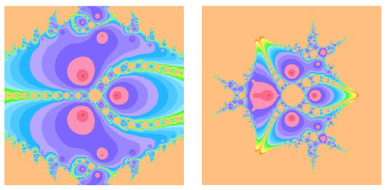
Figure 1. Basin of attractions for (1) with $\beta =0.1$ on $g\left(z\right)=z^3-1$ (left), $g\left(z\right)=z^4-1$ (right).

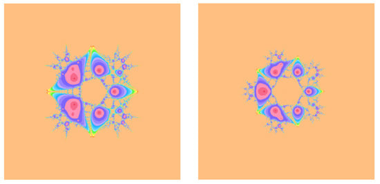
Figure 2. Basin of attractions for (1) with $\beta =0.1$ on $g\left(z\right)=z^5-1$ (left), $g\left(z\right)=z^6-1$ (right).

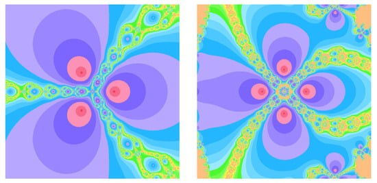
Figure 3. Basin of attractions for (12) with $\beta =p=0.01$ on $g\left(z\right)=z^3-1$ (left), $g\left(z\right)=z^4-1$ (right).

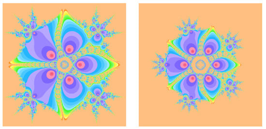
Figure 4. Basin of attractions for (12) with $\beta =p=0.01$ on $g\left(z\right)=z^5-1$ (left), $g\left(z\right)=z^6-1$ (right).

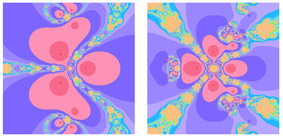
Figure 5. Basin of attractions for (19) with ${\beta }_0=p_0=0.1$ on $g\left(z\right)=z^3-1$ (left), $g\left(z\right)=z^4-1$ (right).

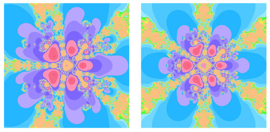
Figure 6. Basin of attractions for (19) with ${\beta }_0=p_0=0.1$ on $g\left(z\right)=z^5-1$ (left), $g\left(z\right)=z^6-1$ (right).

4. Computational Results

Here, we present computational experiments that demonstrate the practical performance of the newly developed Steffensen-type schemes, both with and without memory. All computations were carried out using Mathematica 13.3 with 1500-digit floating-point precision to observe the asymptotic convergence behavior and to avoid premature rounding errors that may obscure the higher-order convergence phenomenon. The results presented here are entirely consistent with the theoretical analysis performed in Section 2 and Section 3, confirming the predicted R-orders, the enhanced convergence radii, and the dynamical robustness of the proposed methods.

To illustrate the advantages of the self-accelerating parameters and the memory mechanism, we consider the oscillatory test function

$$g\left(x\right)=(x-1)\left(x^{10}+x^3+1\right)\sin \left(x\right),$$

(61)

which is known to be challenging for many iterative solvers due to its rapidly oscillating nature and its combination of polynomial and transcendental components. The function has a simple root at $\alpha =1$, but the surrounding landscape contains multiple oscillatory extrema and steep curvature variations, making it a good benchmark for convergence speed and sensitivity to initial guesses.

To visualize the numerical behavior, the iterative trajectories are plotted in Figure 7, where the left frame shows convergence from a moderate initial approximation and the right frame illustrates robustness from a distant starting point. The parameters ${\beta }_0$, $p_0$, and the initial guess $x_0$ used for each scheme are explicitly stated in the figure captions. The simulations reveal that the method with memory not only converges more quickly but also maintains stable behavior in regions where the derivative-free method without memory struggles to converge or becomes sensitive to perturbations.

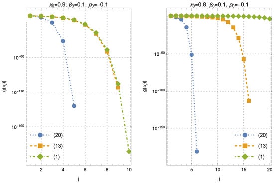
Figure 7. Numerical convergence results for different values of the initial approximations.

The figure shows the residual histories for the test problem (61) using the three derivative-free iterations (1) (Equation $\left(1\right)$, green diamonds), (12) (Equation $\left(13\right)$, orange squares), and the proposed with-memory scheme (19) (Equation $\left(20\right)$, blue circles). In each panel, the vertical axis reports the residual magnitude $\left|g\right(x_j\left)\right|$ on a logarithmic scale versus the iteration index j. Left panel: Starting from the moderate initial approximation $x_0=0.9$ with ${\beta }_0=0.1$ and $p_0=-0.1$, all three schemes converge; however, the with-memory method $\left(20\right)$ produces a markedly steeper decay of $\left|g\right(x_j\left)\right|$, reaching a near-machine residual level within only a few iterations, whereas $\left(1\right)$ and $\left(13\right)$ require substantially more steps to attain comparable residual reductions. Right panel: For the more challenging initial approximation $x_0=0.8$ (with the same initialization ${\beta }_0=0.1$, $p_0=-0.1$), the with-memory scheme $\left(20\right)$ still converges rapidly, the two-parameter method without memory $\left(13\right)$ converges but much more slowly, and the classical Steffensen-type iteration $\left(1\right)$ exhibits stagnation (no visible residual decrease) over the displayed iteration range. Overall, the two panels illustrate that incorporating memory not only accelerates the asymptotic residual decay but also improves robustness with respect to the choice of the initial approximation.

This is consistent with the enlarged attraction basins documented in Section 3, which demonstrate that the interpolation-based parameter updates reinforce the stability properties of the scheme. The numerical experiments support the theoretical findings of Section 2 and Section 3 in two complementary ways. First, for the benchmark (61), the proposed memory-based scheme exhibits a faster residual decay and improved robustness with respect to the initial approximation when compared to the memoryless competitors. Second, the basin-of-attraction study in Section 3 indicates enlarged convergence regions and fewer nonconvergent initial conditions for the with-memory iteration on the tested polynomial families. These results provide evidence of improved efficiency and dynamical robustness.

Before ending this section, we evaluate the performance of the discussed schemes with some other recently proposed schemes [31] as follows ($q_j\in [0, 1]$):

• Moser–Secant method:

  $$\begin{array}{c}\hfill \left\{\begin{array}{c}{x}_{j+1}=x_j-{\overline{A}}_{j}g\left(x_j\right),j\ge 0,\hfill \\ y_{j+1}=x_j+q_j(x_{j+1}-x_j),\hfill \\ {\overline{K}}_{j+1}={\displaystyle \frac{g\left(y_{j+1}\right)-g\left(x_{j+1}\right)}{y_{j+1}-x_{j+1}}},\hfill \\ {\overline{A}}_{j+1}=2{\overline{A}}_j-{\overline{A}}_j{\overline{K}}_{j+1}{\overline{A}}_j,\hfill \end{array}\right.\end{array}$$

  (62)
• Moser–Kurchatov method:

  $$\begin{array}{c}\hfill \left\{\begin{array}{c}{x}_{j+1}=x_j-{\overline{A}}_{j}g\left(x_j\right),j\ge 0,\hfill \\ y_{j+1}=x_j+q_j(x_{j+1}-x_j),\hfill \\ {\overline{K}}_{j+1}={\displaystyle \frac{g(2y_{j+1}-x_{j+1})-g\left(x_{j+1}\right)}{(2y_{j+1}-x_{j+1})-x_{j+1}}},\hfill \\ {\overline{A}}_{j+1}=2{\overline{A}}_j-{\overline{A}}_j{\overline{K}}_{j+1}{\overline{A}}_j.\hfill \end{array}\right.\end{array}$$

  (63)

We have chosen for the initial approximation $x_0=1.2$. The results are provided in Table 1. The schemes (62) and (63) are useful for systems of nonlinear equations, but they are sensitive to the choice of ${\overline{A}}_j$ as an approximation of the first derivative, and thus their convergence radii are lower than that of the Steffensen-type method with memory. Here, we have chosen ${\overline{A}}_0=f^{\prime }{\left(x_0\right)}^{-1}$ and $q_j=1/2$. Numerical results confirm the efficiency of (19).

Table 1. Convergence comparisons for $x_0=1.2$ to solve (61).

	(1)	(12)	(19)	(62)	(63)
$\left|g\right(x_2\left)\right|$	0.5915	0.5911	0.1375	0.2715	0.2934
$\left|g\right(x_3\left)\right|$	0.2549	0.2545	0.0013	0.1271	0.1471
$\left|g\right(x_4\left)\right|$	0.07539	0.0750	$5.213\times {10}^{-11}$	0.0500	0.0639
$\left|g\right(x_5\left)\right|$	0.0104	0.0102	$2.889\times {10}^{-37}$	0.013889	0.0211
$\left|g\right(x_6\left)\right|$	0.0002	0.0002	$5.167\times {10}^{-130}$	0.0019	0.0042
$\left|g\right(x_7\left)\right|$	$1.597\times {10}^{-7}$	$1.479\times {10}^{-7}$	-	0.00007	0.0003
$\left|g\right(x_8\left)\right|$	$6.298\times {10}^{-14}$	$5.362\times {10}^{-14}$	-	$2.450\times {10}^{-7}$	$4.606\times {10}^{-6}$
$\left|g\right(x_9\left)\right|$	$9.791\times {10}^{-27}$	$7.041\times {10}^{-27}$	-	$2.024\times {10}^{-11}$	$3.875\times {10}^{-9}$
Rates	2.00	2.00	3.53	1.61	1.61

5. Concluding Summary

In this work, we improved and analyzed a new Steffensen-type iterative scheme equipped with two free parameters and a memory-based acceleration mechanism. The derivative-free method without memory was shown to achieve optimal quadratic convergence, while its extension with memory attained an R-order of $3.56155$ without requiring any additional functional evaluations. By employing Newton interpolation polynomials to approximate the self-accelerating parameters, the proposed scheme demonstrated improved local convergence behavior, enhanced efficiency index, and enlarged attraction basins. Numerical experiments and dynamical analyses confirmed that the new method performs efficiently.

Future research will focus on broadening the applicability of the proposed framework to systems of nonlinear equations and matrix equations. Some other scholars may study an alternative approximation tools, such as Padé-type rational interpolants or machine-learning-based parameter estimators for enhanced convergence.

References

- Shil, S.; Nashine, H.K.; Soleymani, F. On an inversion-free algorithm for the nonlinear matrix problem . Int. J. Comput. Math. 2022, 99, 2555–2567. [Google Scholar] [CrossRef]
- Bini, D.A.; Iannazzo, B. Computational aspects of the geometric mean of two matrices a survey. Acta Sci. Math. 2024, 90, 349–389. [Google Scholar] [CrossRef]
- Dehdezi, E.K.; Karimi, S. A fast and efficient Newton-Shultz-type iterative method for computing inverse and Moore-Penrose inverse of tensors. J. Math. Model. 2021, 9, 645–664. [Google Scholar]
- Noda, T. The Steffensen iteration method for systems of nonlinear equations. Proc. Jpn. Acad. 1987, 63, 186–189. [Google Scholar] [CrossRef]
- Steffensen, J.F. Remarks on iteration. Skand. Aktuarietidskr. 1933, 16, 64–72. [Google Scholar] [CrossRef]
- Mehta, B.; Parida, P.K.; Nayak, S.K. Convergence analysis of higher order iterative methods in Riemannian manifold. Rend. Circ. Mat. Palermo II. Ser 2026, 75, 8. [Google Scholar] [CrossRef]
- Song, Y.; Soleymani, F.; Kumar, A. Finding the geometric mean for two Hermitian matrices by an efficient iteration method. Math. Methods Appl. Sci. 2025, 48, 7188–7196. [Google Scholar] [CrossRef]
- Zhang, K.; Soleymani, F.; Shateyi, S. On the construction of a two-step sixth-order scheme to find the Drazin generalized inverse. Axioms 2025, 14, 22. [Google Scholar] [CrossRef]
- Traub, J.F. Iterative Methods for the Solution of Equations; Prentice-Hall: New York, NY, USA, 1964. [Google Scholar]
- Kung, H.T.; Traub, J.F. Optimal order of one–point and multi–point iteration. J. ACM 1974, 21, 643–651. [Google Scholar] [CrossRef]
- Arora, H.; Cordero, A.; Torregrosa, J.R. On generalized one-step derivative-free iterative family for evaluating multiple roots. Iran. J. Numer. Anal. Optim. 2024, 14, 291–314. [Google Scholar]
- Ostrowski, A.M. Solution of Equations and Systems of Equations; Academic Press: New York, NY, USA, 1966. [Google Scholar]
- Torkashvand, V. A two-step method adaptive with memory with eighth-order for solving nonlinear equations and its dynamic. Comput. Methods Differ. Equ. 2022, 10, 1007–1026. [Google Scholar]
- Khaksar Haghani, F. A modified Steffensen’s method with memory for nonlinear equations. Int. J. Math. Model. Comput. 2015, 5, 41–48. [Google Scholar]
- Chicharro, F.I.; Cordero, A.; Garrido, N.; Torregrosa, J.R. Stability and applicability of iterative methods with memory. J. Math. Chem. 2019, 57, 1282–1300. [Google Scholar] [CrossRef]
- Džunić, J.; Petković, M.S. On generalized biparametric multipoint root finding methods with memory. J. Comput. Appl. Math. 2014, 255, 362–375. [Google Scholar] [CrossRef]
- Soleymani, F.; Vanani, S.K. A modified eighth-order derivative-free root solver. Thai. J. Math. 2012, 10, 541–549. [Google Scholar]
- Yilmaz, N. Introducing three new smoothing functions: Analysis on smoothing-Newton algorithms. J. Math. Model. 2024, 12, 463–479. [Google Scholar]
- Dehghani-Madiseh, M. A family of eight-order interval methods for computing rigorous bounds to the solution to nonlinear equations. Iran. J. Numer. Anal. Optim. 2023, 13, 102–120. [Google Scholar]
- Sreedeep, C.D.; Argyros, I.K.; Gopika Dinesh, K.C.; Shrestha, N.; Argyros, M. Convergence analysis of a power series based iterative method having seventh order of convergence. Mat. Stud. 2025, 64, 179–193. [Google Scholar] [CrossRef]
- George, S.; Grammont, M.M.L. Derivative-free convergence analysis for Steffensen-type schemes for nonlinear equations. Appl. Numer. Math. 2026, 223, 101–120. [Google Scholar] [CrossRef]
- Wang, X.; Guo, S. Dynamic analysis of a family of iterative methods with fifth-order convergence. Fractal Fract. 2025, 9, 783. [Google Scholar] [CrossRef]
- Ogbereyivwe, O.; Izevbizua, O. A three-free-parameter class of power series based iterative method for approximation of nonlinear equations solution. Iran. J. Numer. Anal. Optim. 2023, 13, 157–169. [Google Scholar]
- Soleymani, F. Some optimal iterative methods and their with memory variants. J. Egypt. Math. Soc. 2013, 21, 59–67. [Google Scholar] [CrossRef]
- Kiyoumarsi, F. On the construction of fast Steffensen–type iterative methods for nonlinear equations. Int. J. Comput. Meth. 2018, 15, 1850002. [Google Scholar] [CrossRef]
- Getz, C.; Helmstedt, J. Graphics with Mathematica Fractals, Julia Sets, Patterns and Natural Forms; Elsevier: Amsterdam, The Netherlands, 2004. [Google Scholar]
- Zhu, J.; Li, Y.; Li, Y.; Liu, T.; Ma, Q. Fourth-order iterative algorithms for the simultaneous calculation of matrix square roots and their inverses. Mathematics 2025, 13, 3370. [Google Scholar] [CrossRef]
- Howk, C.L.; Hueso, J.L.; Martínez, E.; Teruel, C. A class of efficient high–order iterative methods with memory for nonlinear equations and their dynamics. Math. Meth. Appl. Sci. 2018, 41, 7263–7282. [Google Scholar] [CrossRef]
- Wang, S.; Wang, Z.; Xie, W.; Qi, Y.; Liu, T. An accelerated sixth-order procedure to determine the matrix sign function computationally. Mathematics 2025, 13, 1080. [Google Scholar] [CrossRef]
- Mureşan, M. Introduction to Mathematica with Applications; Springer: Cham, Switzerland, 2017. [Google Scholar]
- Argyros, I.K.; Shakhno, S.M.; Shunkin, Y.V. On an iterative Moser–Kurchatov method for solving systems of nonlinear equations. Mat. Stud. 2025, 63, 88–97. [Google Scholar] [CrossRef]
Disclaimer/Publisher’s Note: The statements, opinions and data contained in all publications are solely those of the individual author(s) and contributor(s) and not of MDPI and/or the editor(s). MDPI and/or the editor(s) disclaim responsibility for any injury to people or property resulting from any ideas, methods, instructions or products referred to in the content. |
© 2026 by the authors. Licensee MDPI, Basel, Switzerland. This article is an open access article distributed under the terms and conditions of the Creative Commons Attribution (CC BY) license.