Two-Stage Genetic-Based Optimization for Resource Provisioning and Scheduling of Multiple Workflows on the Cloud Under Resource Constraints

Abstract

Resource provisioning and scheduling are essential challenges in handling multiple workflow requests within cloud environments, particularly given the constraints imposed by limited resource availability. Although workflow scheduling has been extensively studied, few methods effectively integrate resource provisioning with scheduling, especially under cloud resource limitations and the complexities of multiple workflows. To address this challenge, we propose an innovative two-stage genetic-based optimization approach. In the first stage, candidate cloud resources are selected for the resource pool under the given resource constraints. In the second stage, these resources are provisioned and task scheduling is optimized on the selected resources. A key advantage of our approach is that it reduces the search space in the first stage through a novel encoding scheme that enables a caching strategy, in which intermediate results are stored and reused to enhance optimization efficiency in the second stage. The proposed solution is evaluated through extensive simulation experiments, assessing both resource selection and task scheduling across a diverse range of workflows. The results demonstrate that the proposed approach outperforms existing algorithms, particularly for highly parallel workflows, highlighting its effectiveness in managing complex workflow scheduling under resource-constrained cloud environments.

1. Introduction

Business analysis and scientific computing applications often handle large volumes of data. To minimize processing times, data are partitioned and processed in parallel. Intermediate data are then transferred to the sequential steps of the applications. These applications, which involve both parallel and sequential tasks, are typically modeled as workflows [1]. These complex computing tasks centered around the analysis of large-scale data sets require significant computing power [2]. As numerous teams or engineers often conduct different tasks simultaneously, there is a critical need to manage multiple workflows effectively. In this context, cloud computing becomes an indispensable solution, providing the resources required to execute these complex workflows.

In cloud environments, resource allocation is tailored to specific requirements and billed according to usage duration, reflecting the elasticity and pay-per-use characteristics of cloud services. Under-provisioning resources decreases system performance, whereas over-provisioning leads to idle resources [1]. It is important to determine the types and quantities of required resources accurately and allocate an appropriate amount to each workflow as needed, rather than reserving a fixed number in advance [3]. Given the complexity of cloud environments and workflow structures, designing scheduling algorithms specifically for multiple workflows on cloud resources becomes essential [4]. The challenge in cloud resource provisioning and scheduling lies in determining the duration, type, and number of virtual machines (VMs) to rent and release, adapted to the applications’ characteristics [5].

Existing works predominantly concentrate on workflow scheduling with static resource provisioning [6,7], wherein the number of VMs is established before scheduling and remains constant during execution. Estimating VM requirements is challenging due to workflow variability. Unlimited resources expedite completion but cause low utilization and high costs [8]. Resource demand is also influenced by the specific applications in use. Moreover, cloud platforms often set quotas on the number of instances that can be deployed to safeguard against issues like improper resource deployments or excessive consumption. Consequently, there is an upper limit on the number of VM instances for each resource type and a collective maximum limit on the total number of VM instances across all resource types.

Efficient resource provisioning and task mapping are essential for balancing costs and makespan in cloud workflows. From a user’s perspective, the goal is to rent a reasonable number and types of resources at minimal cost to meet these requirements. Meanwhile, from each workflow’s perspective, the objective is to complete execution as quickly as possible. Overall, the aim is to execute all workflows within a reasonable duration while minimizing costs.

To tackle the challenges of provisioning and scheduling in cloud environments under resource constraints, we propose a two-stage GA-based provisioning and scheduling method (2SG-PS). Although several GA-based methods have been proposed for workflow scheduling and resource provisioning, most either assume a fixed resource pool or optimize provisioning and scheduling in a single stage, which leads to a very large search space and makes it difficult to explicitly enforce strict instance-level limits on the number of VM instances. This strategy employs a genetic algorithm to minimize both the total cost of cloud resources and the average makespan of individual workflows. The first stage concentrates on optimizing a candidate resource pool, determining the number of resource instances among various types of available resources while adhering to the given resource constraints. The second stage focuses on selecting resource instances from the candidate pool and refining task scheduling, with an emphasis on evaluating the total cost and the average makespan of individual workflows. This approach efficiently narrows the search space by encoding only the instance numbers for each resource type in the first stage, enhancing caching possibilities for the second stage. Furthermore, we propose a new ranking and selection procedure for the two-stage optimization, selecting Pareto-optimal solutions based on the second-stage outcomes, thereby ensuring more effective resource management. The major contributions of this paper are summarized as follows:

• A two-stage optimization approach for resource provisioning and scheduling multiple workflows under resource constraints, comprising two independent processes: (i) candidate resource pool optimization and (ii) joint resource provisioning and task scheduling.
• Two encoding schemes specifically tailored for resource provisioning and scheduling.
• A novel ranking and selection procedure for the proposed two-stage optimization framework.
• An extensive experimental evaluation using both randomly generated workflows and real scientific workflows.

The remainder of this paper is organized as follows. A review of related works is summarized in Section 2, followed by the problem description and formulation in Section 3. The algorithms proposed in this paper are described in Section 4. Simulation experiments based on different algorithms are performed and results are compared in Section 5. Finally, conclusions and future works are presented in Section 6.

2. Literature Review

The problem of scheduling workflow on distributed resources has been extensively studied in recent years. Many studies have addressed this problem from different perspectives. Table 1 summarizes scheduling on distributed resources. Each work is distinguished by task types and resource types. In the following, we briefly review representative approaches in each category.

Table 1. Summary of Scheduling on Distributed Resources.

Literature	Task Types		Resource Pool Types
	Independent Tasks	Dependent Tasks (Workflow)	Fixed	Flexible
Abrishami et al. [9]		✓	✓
Topcuoglu et al. [10]		✓	✓
Chen and Zhang [11]		✓	✓
Li et al. [12]		✓	✓
Xia et al. [13]		✓	✓
Kumar et al. [14]	✓			✓
Ghobaei-Arani and Shahidinejad [15]	✓			✓
Mao et al. [16]	✓			✓
Bi et al. [17]	✓			✓
Byun et al. [8]		✓		✓
Li and Cai [1]		✓		✓
Arabnejad et al. [18]		✓		✓
Faragardi et al. [19]		✓		✓
Garg et al. [20]		✓		✓
Rajasekar and Palanichamy [21]		✓		✓
Rodriguez and Buyya [22]		✓	✓
Zhu et al. [23]		✓		✓
Malawski et al. [24]		✓		✓

Most existing research assumes that a limited, fixed pool of computing resources is available. For instance, Abrishami et al. [9] developed a heuristic algorithm, partial critical paths, for cloud environments and proposed two workflow scheduling algorithms. Two novel scheduling algorithms, the Heterogeneous Earliest-Finish-Time (HEFT) algorithm and the Critical-Path-on-a-Processor (CPOP) algorithm, were presented in [10] for workflow scheduling. Chen and Zhang [11] proposed an ant colony optimization algorithm to schedule large-scale workflows with various QoS parameters. Li et al. [12] introduced a cloud-based, three-stage workflow scheduling model and employed symbiotic organisms search-based algorithms to optimize an integrated objective function, aiming to minimize completion time and cost while maximizing accuracy. Xia et al. [13] proposed an initialization scheduling sequence scheme based on task data sizes to improve search efficiency in a multi-objective genetic algorithm for workflow scheduling problems. The above-summarized research tends to focus only on scheduling under the assumption that a fixed pool of resources is used execution. The number and types of resources cannot be dynamically adjusted to variable workflows or requirements, and hence fail to provide provisioning strategies that adapt to different situations.

Resource provisioning has recently gained attention, with most methods focusing on independent tasks rather than workflows. Kumar et al. [14] proposed an improved binary particle swarm optimization to optimize various QoS metrics such as makespan, energy consumption, and execution cost. Ghobaei-Arani and Shahidinejad [15] proposed a clustering-based resource approach. First, the workload was clustered using a GA algorithm and fuzzy C-means method, and resource scaling is then determined using a gray wolf optimizer (GWO). Mao et al. [16] proposed a cloud auto-scaling mechanism to change the scale and the type of VMs based on real-time workloads, and the objective was to minimize renting costs while meeting performance requirements. Bi et al. [17] proposed allocating heterogeneous resources to requests using dynamic fine-grained resource provisioning to minimize the number of VMs. These methods only work for independent tasks and do not consider dependencies among tasks within a workflow. Without support for precedence and data-flow dependencies, these approaches cannot exploit critical-path information or inter-task communication costs, and thus are not suitable for complex workflow applications.

Meanwhile, other methods have considered resource provisioning and scheduling within a workflow model. Byun et al. [8] proposed a heuristic algorithm,  partitioned balanced time scheduling, to determine the best number of computing resources per time charge unit required to execute a workflow within a given deadline, minimizing the cost during the entire application lifetime. The algorithm was only conducted in each time partition rather than the whole workflow and only one type of resource is assumed. Li and Cai [1] proposed a multiple rule-based heuristics for provisioning elastic cloud resources for workflows to minimize total resource renting costs, using two main steps: dividing the workflow deadline into task deadlines and scheduling tasks to resources constrained by task deadlines. The resource renting cost was minimized by applying auto-scaling mechanisms. Arabnejad et al. [18] proposed a new heuristic scheduling algorithm, budget and deadline-aware scheduling, constrained by both budget and deadline. Faragardi et al. [19] proposed a novel resource provisioning mechanism and a workflow scheduling algorithm that minimize makespan of the given workflow subject to a budget constraint. The limitation is that the resource provisioning mechanism strictly relies on an hourly-based cost constraint, which cannot be used by other models. Garg et al. [20] proposed an energy- and resource-efficient workflow scheduling algorithm to schedule the workflow tasks and dynamically deploy/un-deploy resources. The limitation is that the threshold must be known to decide when to deploy or un-deploy resources. Rajasekar and Palanichamy [21] presented an adaptive resource provisioning and scheduling algorithm for scientific workflows. If no free resources are available for the current task, a new resource should be leased. However, this approach cannot be applied to a global decision-making process. Although these heuristic approaches can yield optimal solutions, they are problem-specific and require custom design for each scenario. In addition, the computational complexity of heuristic algorithms increases exponentially when the complexity of the problem increases linearly. Moreover, most of these heuristic methods are tailored to single-workflow settings and do not jointly optimize provisioning and scheduling for multiple concurrent workflows under global resource constraints.

In contrast, meta-heuristic algorithms provide general, global search strategies and are used to find near-optimal scheduling schemes in NP-hard optimization problems Shishido et al. [25]. For example, Rodriguez and Buyya [22] proposed a resource provisioning and scheduling strategy based on particle swarm optimization for workflows with a predefined resource pool. Although the pool can be adjusted based on the number of parallel tasks in workflows, it makes an initial resource provisioning pool in advance and is unchanged during the scheduling optimization for workflow. The disadvantage is that the predefined static resource pool cannot avoid unnecessary resource occupation. Zhu et al. [23] proposed an evolutionary multi-objective optimization algorithm to solve the problem of single workflow scheduling and resource provisioning. However, these algorithms remain limited to single workflow scheduling.

More recently, several multi-objective and hybrid meta-heuristic methods have been proposed for workflow and task scheduling [26,27,28,29]. Khan and Rasool [26] use a grey-wolf optimizer to minimize makespan, energy consumption, and monetary cost for independent tasks on a fixed set of virtual machines. Rathi et al. [27] and Mikram et al. [29] combine genetic search with other heuristics to schedule workflows in fog–cloud or cloud data-center environments, and Cai et al. [28] develop a multi-objective evolutionary scheduler for deadline-constrained workflows in multi-cloud environments. However, these studies still assume a given (or virtually elastic) resource pool and do not explicitly decide how many instances of each VM type should be provisioned for multiple concurrent workflows under strict capacity limits.

Resource provisioning and scheduling optimization for multiple workflows has also been studied, particularly with respect to resource scheduling. Malawski et al. [24] considered workflow ensembles rather than individual workflows and proposed static and dynamic provisioning and scheduling methods. The goal is to complete as many high-priority workflows as possible under a fixed budget and deadline. However, they consider budget as a constraint rather than cost minimization as a goal, and only one resource type was considered.

In summary, existing scheduling and provisioning approaches either assume a fixed resource pool, optimize provisioning and scheduling in a single stage (leading to a large search space), or focus on independent tasks or single workflows. Recent multi-objective and hybrid meta-heuristic methods [26,27,28,29] have advanced workflow scheduling but still do not jointly optimize resource provisioning and scheduling for multiple workflows under strict per-type and global VM-instance limits. In contrast, our 2SG-PS method targets multiple dependent workflows sharing a constrained VM pool and (i) optimizes the resource-pool composition under explicit instance constraints in Stage 1 and (ii) refines scheduling in Stage 2 while jointly minimizing total cost and average makespan, thereby filling this gap.

3. Problem Formulation

This section begins with workflow and resource modeling, followed by a discussion on task scheduling and objective formulation. The symbols and variables used in this paper are summarized in Table 2.

Table 2. Symbols and variables.

Symbol	Description
N	The number of workflows.
W	The set of workflows.
T	The set of all tasks in W.
$T_n$	The set of tasks in workflow $W_n$.
$t_i$	A task in the set of tasks.
$D_n$	The set of directed edges in workflow $W_n$.
$\left|T\right|$	The number of tasks in the workflow set.
M	The number of types of cloud computing resources.
R	The set of cloud computing resources.
$R_m$	The set of resource instances for resource type m.
$TS{T}_i$	The tentative start time of task $t_i$.
$AS{T}_i^r$	The actual start time of task $t_i$ on resource r.
$CT$	The communication time.
$FT$	The finish time.
$D{S}_{hi}$	The data size transferred from $t_h$ to $t_i$.
$B{W}_r$	The bandwidth of resource r.
$E{T}_i^r$	The execution time of task $t_i$ on resource r.
$W{L}_i$	The workload of task $t_i$.
$CP{U}_r$	The CPU capacity of resource r.
$Mk\left(W_i\right)$	The makespan of workflow $W_i$.
$C_r$	The cost to lease a resource instance r.
$\mathbf{C}$	The total cost.
${\overline{R}}_m$	The upper bound on the number of resource instances of type m.
$\overline{R}$	The upper bound on the total number of provisioned resource instances.
$RN$	The number of resource instances.

3.1. Workflow and Resource Modeling

Suppose a user possesses a set of N workflows, designated as $W=\{W_0,\dots ,W_{N-1}\}$, which are to be executed on the cloud. Each workflow is represented by a direct acyclic graph (DAG), $W_n=(T_n,D_n)$, where $T_n$ is the set of tasks that make up the workflow, and $D_n$ is a set of directed edges which is denoted by $D_n=\left\{(t_i,t_j)\right|t_i,t_j\in T_n\}$. A task is ready for execution when all preceding tasks are complete and the necessary data is available. Hence, if the execution of task $t_j$ can start only after $t_i$ finishes its execution, this means that there is a precedence constraint between $t_i$ and $t_j$. T is denoted as the set of all tasks in W, such that $T={\bigcup }_{W_n(T_n,D_n)\in W}{T}_n$. The number of tasks in the workflow set is denoted as $\left|T\right|$.

The predecessors of a task $t_j$ are defined as

$$pred\left(t_j\right)=\left\{t_i\right|(t_i,t_j)\in D_n\}$$

(1)

In the workflow set W, $T_{entry}$ denote the set of tasks without any preceding tasks that satisfy

$$\forall t_i\in T_{entry}:pred\left(t_i\right)=\varnothing$$

(2)

and $T_{exit}$ denote the set of tasks without any succeeding tasks that satisfy

$$\forall t_i\in T,pred\left(t_i\right)\cap T_{exit}=\varnothing$$

(3)

Concerning the resource set, we consider M distinct types of cloud computing resources, represented as $\mathbf{R}=\{R_0,\dots ,R_{M-1}\}$ each characterized by specific attributes such as processing capabilities and processing costs. Here, $R_m$ is the set of resource instances corresponding to resource type m. The aggregate resource instances $R={\bigcup }_{R_m\in \mathbf{R}}{R}_m$ represents all instances across resource types.

Each resource type corresponds to a virtual machine (VM) configuration, characterized by its CPU capacity $CP{U}_r$ (operations per time unit) and unit-time cost ${\widehat{C}}_r$ (as defined in Equations (6) and (10)). In our two-stage optimization framework, Stage 1 decides how many VM instances of each type are provisioned (i.e., the size of $R_m$ for each m), and Stage 2 assigns tasks to these provisioned instances and constructs feasible schedules.

We assume that VM instances are elastically provisioned for the duration of their actual use and remain available from the start time of the first assigned task until the completion time of the last assigned task (cf. Section 3.3.2). Running tasks are not migrated between VM instances; once a task starts execution on a VM, it runs to completion on that VM without interruption. This static task-to-VM assignment is a common assumption in cloud workflow scheduling, as it avoids the overhead and complexity of live task migration.

3.2. Task Scheduling

For the scheduling of tasks, it is necessary to compute the start and finish times for each task on the assigned resources. The process is based on certain assumptions:

• Multiple workflows are randomly submitted in batches, and a scheduling sequence for tasks across all workflows is established.
• Once started, each task continues without interruption until it reaches completion.
• Each task runs exclusively on a single resource at a certain occupied time.

Initially, the tentative start time $TS{T}_i$ for task $t_i$ is determined, signifying the earliest start time for execution:

$$TS{T}_i=\left\{\begin{array}{cc}0\hfill & \mathrm{if}{t}_i\in T_{entry}\hfill \\ \underset{t_h\in pred\left(t_i\right)}{max}(F{T}_h^r+C{T}_{hi}^{rs})\hfill & \mathrm{if}{t}_i\notin T_{entry}\hfill \end{array}\right.$$

(4)

where $r,s\in R$. If $t_i$ is an entry task, $TS{T}_i=0$. $C{T}_{hi}^{rs}$ is the communication time between two tasks $t_h$ to $t_i$ which are executed on resource instance r and s, respectively. $F{T}_h^r$ is the finish time of $t_h$ executing on resource r.

The communication time between $t_h$ to $t_i$, $C{T}_{hi}^{rs}$, is defined as follows:

$$C{T}_{hi}^{rs}=\left\{\begin{array}{cc}0\hfill & \mathrm{if}r=s\hfill \\ {\displaystyle \frac{D{S}_{hi}}{min(B{W}_r,B{W}_s)}}\hfill & \mathrm{if}r\ne s\hfill \end{array}\right.$$

(5)

where $D{S}_{hi}$ is the data size transferred from $t_h$ to $t_i$; $B{W}_r$ is the bandwidth of the resource r. If $t_h$ and $t_i$ are executing on the same resource r, then there is no additional communication time. Otherwise, it is determined by the data size to be transferred between resource r and s, constrained by the bandwidth between the resources.

A gap is an idle time interval on a resource between scheduled tasks. To schedule a new task $t_i$, we identify suitable gaps where the task can fit.

Step 1: Execution Time Calculation. The execution time of task $t_i$ on resource r is:

$$E{T}_i^r={\displaystyle \frac{W{L}_i}{CP{U}_r}},$$

(6)

where $W{L}_i$ is the task workload (in operations) and $CP{U}_r$ is the resource capacity (operations per time unit).

Step 2: Gap Identification and Start Time Determination. The actual start time $AS{T}_i^r$ depends on gap availability. Let $t_a$ and $t_b$ be consecutive tasks on resource r, and $t_l$ be the last scheduled task. We define the gap size between consecutive tasks as:

$${\Delta }_{ab}=AS{T}_b^r-F{T}_a^r,$$

which represents the idle time between when $t_a$ finishes and $t_b$ starts.

The scheduling algorithm searches for the earliest feasible slot:

$$AS{T}_i^r=\left\{\begin{array}{cc}F{T}_a^r,\hfill & \mathrm{if}{\Delta }_{ab}\ge E{T}_i^r\wedge TS{T}_i<F{T}_a^r,\hfill \\ TS{T}_i,\hfill & \mathrm{if}{\Delta }_{ab}\ge E{T}_i^r\wedge TS{T}_i\ge F{T}_a^r,\hfill \\ F{T}_l^r,\hfill & \mathrm{if}\forall (t_a,t_b):{\Delta }_{ab}<E{T}_i^r\wedge TS{T}_i<F{T}_l^r,\hfill \\ TS{T}_i,\hfill & \mathrm{if}\forall (t_a,t_b):{\Delta }_{ab}<E{T}_i^r\wedge TS{T}_i\ge F{T}_l^r.\hfill \end{array}\right.$$

(7)

Interpretation of Scheduling Cases:

• Gap-fitting cases (when $\exists {\Delta }_{ab}\ge E{T}_i^r$):

  (a)

  Early arrival ($TS{T}_i<F{T}_a^r$): The task is ready before the gap opens. It must wait until $F{T}_a^r$ when the resource becomes available.

  (b)

  On-time arrival ($TS{T}_i\ge F{T}_a^r$): The task arrives after the gap opens. It can start immediately at its tentative start time $TS{T}_i$, as the resource is already idle.

• No-gap cases (when $\forall {\Delta }_{ab}<E{T}_i^r$):

  (a)

  Early arrival ($TS{T}_i<F{T}_l^r$): No existing gap can accommodate the task. It must wait until all currently scheduled tasks complete, starting at $F{T}_l^r$.

  (b)

  Late arrival ($TS{T}_i\ge F{T}_l^r$): The task arrives after all scheduled tasks complete. The resource is completely free, so the task starts immediately at $TS{T}_i$.

Gap Selection Policy: When multiple suitable gaps exist (multiple ${\Delta }_{ab}\ge E{T}_i^r$), we apply the earliest-fit policy, selecting the gap with the minimum feasible start time to minimize resource idle time.

Step 3: Completion Time. Once scheduled, the task completion time is simply:

$$F{T}_i^r=AS{T}_i^r+E{T}_i^r.$$

(8)

Example: Consider resource r with tasks finishing at times $F{T}_1^r=10$, $F{T}_2^r=25$. A new task with $E{T}_i^r=8$ and $TS{T}_i=12$ would start at $AS{T}_i^r=12$ (case 1b), fitting in the gap $[10,25]$ and completing at $F{T}_i^r=20$.

3.3. Objective Formulation

We aim to solve the following workflow scheduling problem. A set of workflows with a set of tasks in each workflow is submitted to the cloud resources. The problem is to find a schedule S, such that the tasks are scheduled on a set of suitable resource instances, such that $S=\left\{(t_i,r_j)\right\}$ where $t_i\in T$ and $r_j\in R$, based on the objectives under the resource constraint.

Two of the most common objectives for scheduling workflows are makespan and cost. The minimum makespan implies a high execution efficiency. There is more than one workflow in the workflow set, and each workflow aims to be completed with minimal makespan. Hence, the objectives of resource provisioning and allocation are to minimize the mean of the makespan of each workflow and the total cost. The following will introduce these two objectives.

3.3.1. Minimizing Individual Makespan

As stated in the problem formulation, each workflow in $\mathcal{W}$ aims to be completed with minimal makespan. To reflect this per-workflow objective, we use the average makespan as the first optimization goal:

$$\overline{Mk}={\displaystyle \frac{1}{\left|\mathcal{W}\right|}}\sum _{W_i\in \mathcal{W}}Mk\left(W_i\right)$$

(9)

where $Mk\left(W_i\right)$ is the makespan of workflow $W_i$. Minimizing $\overline{Mk}$ encourages every workflow to have a small makespan and penalizes schedules that significantly delay any subset of workflows.

3.3.2. Minimizing Total Cost

To improve the utilization of the leased resources, each resource instance can be shared between tasks belonging to the same or different workflows. The leased resource is only provisioned when the task allocated to it needs to start executing and released when no other tasks from the workflows are allocated to it. Hence, the resource pool is elastic as it scales the resource instances according to the execution of the tasks in the workflows.

When a user submits multiple workflows to the cloud, unlimited resource instances in the cloud will enable the workflows to be completed in the shortest time. However, the pay-per-use billing model is considered in this paper, and partial utilization of the leased VM instance-hour is counted as a full-time period [30]. Unlimited resources may be insufficiently utilized in a billing interval and hence increases rent cost for redundant resources. Hence, apart from makespan, decreasing the monetary cost of execution for all required workflows has always been the other major concern.

First, the cost to lease a resource instance r, $C_r$, is calculated based on the overall execution time of all the tasks allocated to r:

$$\begin{array}{c}\forall (t_a,r),(t_b,s)\in S,\mathrm{where}s=r\hfill \\ C_r=\lceil max\left(F{T}_b^r\right)-min\left(AS{T}_a^r\right)\rceil \times {\widehat{C}}_r\hfill \end{array}$$

(10)

$min\left(AS{T}_a^r\right)$ is the start time of the first task and $max\left(F{T}_b^r\right)$ is the finish time of the last task. The resource is elastic as it is only leased from the start of the first task to the completion of the last task. The total execution time is rounded up to the nearest instance-hour. ${\widehat{C}}_r$ is the cost per time unit for resource instance r.

Next, the total cost, $\mathbf{C}$, is determined by the sum of the cost to lease the required resource instance:

$$\mathbf{C}=\sum _{r\in R}{C}_r$$

(11)

The second objective is to minimize the total cost.

Generally, faster resources are more expensive than slower ones, and vice versa. Hence, minimizing cost may increase makespan. The final solutions should find a trade-off between the two objectives.

3.3.3. Resource Constraints

Typically, cloud providers have quotas and limits on the number of resource instances that can be deployed on the cloud. Quotas are usually user-defined to control resource usage for cost control or to ensure fairness and reduce spikes in usage. Limits are defined by the cloud platform mainly due to system limitations. For example, users may be limited to deployments on a single physical machine, where the number of virtual machine instances is limited by the available physical processing cores. As such, the quotas and limits are modeled as resource constraints. This resource allocation framework is governed by two key constraints:

• For every type of resource, denoted by m, the quantity of resource instances available for allocation is limited by a maximum threshold, ${\overline{R}}_m$. This upper limit ensures that the number of allocated instances, $|R_m|$, does not exceed ${\overline{R}}_m$ (i.e., $|R_m|\le {\overline{R}}_m$).
• There is a ceiling $\overline{R}$ for the number of provisioned resource instances, ensuring that the total $\left|P\right|$, where P represents the set of all provisioned resources, remains within this limit.

4. Proposed Resource Provisioning and Scheduling Method

An effective solution to the elastic resource provisioning and scheduling problem consists of two tightly coupled phases: (i) provisioning a pool of VM instances and (ii) scheduling workflow tasks on this pool. The quality of a schedule is constrained by the chosen resource pool, and the efficiency of a resource pool can only be assessed through the schedules that it supports. In our setting, a candidate resource pool R is first determined, and then a schedule S is constructed that assigns each task to one of the instances in R. The set of actually provisioned resources P is the subset of R that is used by S, so that $P\subseteq R$. Our goal is to jointly decide R and S so as to minimize both the total cost of the provisioned instances and the overall workflow completion times.

4.1. Multi-Objective Optimization Framework

We formulate the resource provisioning and scheduling problem as a bi-objective optimization problem. For a candidate solution x, which represents a resource pool and its corresponding task schedule, we consider the following two objectives.

First, let $Mk(W_i\mid x)$ denote the makespan of workflow $W_i$ under solution x. The average makespan over all workflows is

$$f_1\left(x\right)=\overline{Mk}\left(x\right)={\displaystyle \frac{1}{\left|\mathcal{W}\right|}}\sum _{W_i\in \mathcal{W}}Mk(W_i\mid x).$$

Second, the total cost of the provisioned VM instances is

$$f_2\left(x\right)=C\left(x\right),$$

computed from the leased time and unit-time cost of each VM instance as defined in Section 3.3.2. Thus, the objective vector is

$$\mathbf{f}\left(x\right)=\left(f_1\left(x\right),f_2\left(x\right)\right),$$

subject to the resource constraints on the number of VM instances of each type and the global capacity limit.

To search for trade-off solutions to this bi-objective problem, we adopt the Non-dominated Sorting Genetic Algorithm II (NSGA-II). In NSGA-II, each individual in the population encodes a candidate solution x (a resource-pool configuration in Stage 1 or a resource-aware schedule in Stage 2) and is evaluated with respect to both objectives $\left(f_1\left(x\right),f_2\left(x\right)\right)$. Individuals are ranked by non-dominated sorting, and crowding distance is used to maintain diversity along the Pareto front. Solutions that violate resource constraints are treated as infeasible and are either discarded or regenerated during the evolutionary process. The resulting Pareto set provides a family of provisioning-and-scheduling decisions that represent different trade-offs between average makespan and total cost.

We propose a two-stage optimization method to address the problem of elastic resource provisioning and scheduling, which involves refining S to meet specified objectives. This method is termed the Two-Stage Genetic-Based Resource Provisioning and Scheduling (2SG-PS). The first stage focuses on refining the resource pool, while the second stage concentrates on optimizing the schedule based on the resource pool established in the first stage. Given the complexity of the problem, a genetic-based approach is applied for optimization. The overall method is illustrated in the flowchart shown in Figure 1. We introduce novel encoding schemes and a new selection process in the first stage.

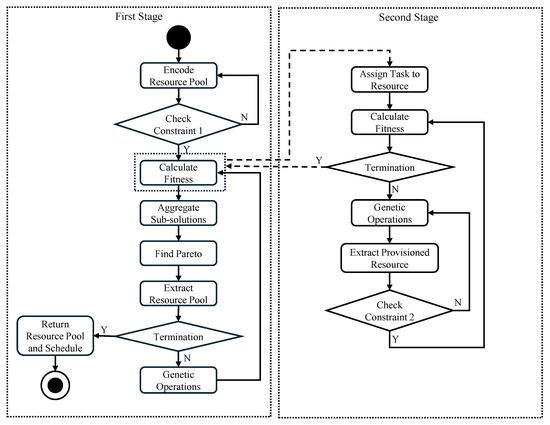
Figure 1. The flowchart of the proposed method.

4.2. Encoding Schemes

The first-stage encoding scheme focuses on optimizing the number of resource instances, denoted by $RN$, for each resource type. This stage involves selecting a potential number of resource instances, yet the actual provisioned resource instances depend on the following task schedule. Each individual in the genetic algorithm for potential resource instance count is represented by a vector of size M and encoded as integers. The range of values possible for each resource type is constrained by ${\overline{R}}_m$. The constraint on the total number of provisioned resource instances is not checked during the first stage. The initial stage proposes a pool of resources, with the actual provisioned resources potentially being less than or equal to this pool. Therefore, the second resource constraint is assessed only in the subsequent stage. Figure 2 exemplifies the proposed encoding scheme. In this scheme, the first layer presents the resource number $RN$, where five types of resources are outlined, namely, $R_0$ to $R_4$. It encodes only the quantity of instances for each resource type; for instance, four instances for $R_0$, three instances for $R_1$, etc.

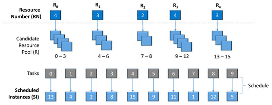
Figure 2. An example of encoding for 2SG-PS.

The second stage is responsible for establishing the schedule, $SI$, to execute the tasks on the provisioned resources. First, the set of potential resource instances, R, is produced based on the quantity of instances received from the first stage. For example, in Figure 2, given the resource number, $RN$, the potential instances for each resource category are as follows: $\{0, 1, 2, 3\}\in R_0$, $\{4, 5, 6\}\in R_1$, $\{7, 8\}\in R_2$, $\{9, 10, 11, 12\}\in R_3$ and $\{13, 14, 15\}\in R_4$. Subsequently, the scheduling assigns tasks to these resource instances, with each task from the workflow being associated with a resource instance.

In the second stage, each individual is encoded by a vector of $\left|T\right|$ size, where $\left|T\right|$ signifies the number of tasks in the workflow set. The tasks are ordered according to the dependencies between the tasks. A schedule of the task mapping is determined based on the resource instances. For instance, task 0 is allocated to the resource instance 13. The same resource instance may be mapped to more than one task, i.e., multiple tasks may be scheduled onto the same resource. This resource pool expands or contracts dynamically in response to workflow demands. For example, the resource instance 13 is provisioned to task 0. Once task 0 is completed, resource instance 13 becomes available for reassignment. If there are no subsequent tasks, it is then relinquished from the resource pool.

Using the above method, we encode only the number of resource instances for each resource type in the first stage. This approach significantly reduces the search space, making the optimization process more efficient. This reduction in complexity not only accelerates the search process but also enhances the algorithm’s ability to find optimal or near-optimal solutions more quickly.

Additionally, this streamlined encoding improves opportunities for caching intermediate results from the second stage. With fewer variables to track, the system can more effectively store and retrieve these intermediate results.

4.3. Stage 1—Optimizing Candidate Resource Pool

For the first stage, we use a Pareto-dominance-based algorithm framework (NSGA-II) to evolve the population. Each resource number is initialized to a value between 0 and ${\overline{R}}_m$ to satisfy Constraint 1. This means that it is also possible that there will be no instances allocated for some resource types.

Algorithm 1 outlines the pseudo-code for the first stage, aiming to generate a new population for the subsequent $g+1$ generation. The process of crossover and mutation operations are first performed on population $R{N}^g$ from the previous generation for each individual. With integers representing the encoding, single-point crossover (SPX) is adopted. If a gene m in $RN$ is selected for mutation, a new valid individual is randomly generated within the range $[0,{\overline{R}}_m)$ with a small probability. This newly generated individual does not undergo direct evaluation as it lacks task-to-resource mapping. Task allocation to resources occurs in the second stage of optimization, yielding a series of sub-solutions. Consequently, each individual possesses a set of performance metrics for every sub-solution from the first stage of optimization. Traditional ranking and selection methods presuppose a corresponding performance metric for each solution. Therefore, a novel ranking and selection approach is proposed to accommodate multiple performance measures for each solution.

Algorithm 1 Stage 1—Generate New Population $g+1$

Require:  Resource Pool ${\mathrm{RN}}^g$ Ensure:  Resource Pool ${\mathrm{RN}}^{g+1}$, Pareto Set $S_p$ 1: $S=\varnothing$ 2: for k = 1 to $pop$ do 3:     ${{\mathrm{RN}}_k}^{\prime }\leftarrow \mathrm{GeneticOps}\left({\mathrm{RN}}_k^g\right)$ 4:     $s\leftarrow \mathrm{OptimizeStage}2\left({{\mathrm{RN}}_k}^{\prime }\right)$ 5:     $S=S\cup s$ 6: end for 7: $S_p=\mathrm{FindPareto}\left(S\right)$ 8: ${\mathrm{RN}}^{g+1}=\varnothing$ 9: for $s\in S_p$ do 10:     ${\mathrm{RN}}^{g+1}={\mathrm{RN}}^{g+1}\cup \mathrm{ExtractResourcePool}\left(s\right)$ 11: end for

4.3.1. Selection Mechanism in Two-Stage Optimization

In Algorithm 1, after optimizing each individual in the second stage, a set of Pareto solutions is obtained for each resource pool (line 4). For instance, as illustrated in Figure 3, there are four individuals from the first stage. After optimizing these individuals in the second stage, the corresponding Pareto sub-solutions are obtained, enumerated as $\{1, 2, 3, 4, 5, 6, 7, 8\}$. These Pareto solutions are consolidated into a set S (line 5). Thereafter, a Pareto set $S_p$ of S is obtained using fast non-dominated sorting (line 7). In Figure 3, sub-solutions $\{3, 5, 8\}$ are identified as the Pareto solutions. Each Pareto solution is mapped back to the initial stage solutions. For instance, sub-solutions $\{3, 5, 8\}$ correspond to stage one solutions $\{1, 2, 4\}$. The unique set of first-stage solutions is then nominated as the first-stage Pareto solutions, which will be evolved in the next generation (line 10).

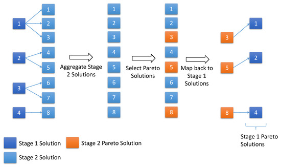
Figure 3. Ranking and Selection for Two-stage Optimization.

4.3.2. Caching Intermediate Results

As the number of resource types is typically much smaller than the number of tasks in the workflow set, i.e., $M<<\left|T\right|$, the search space for $RN$ is considerably smaller. Hence, the population size and number of generations for the first stage can be reduced. Due to the faster convergence in the first stage, the results of the second stage optimization can also be cached to reduce the number of evaluations. To further reduce computational cost, 2SG-PS uses a multi-fidelity approach: during the exploration phase, Stage 2 runs with reduced population and generations (fidelity ratio $=0.3$). After exploration, the top-K resource configurations are re-evaluated with full fidelity to ensure solution quality.

4.4. Stage 2—Optimizing Resource Provisioning and Scheduling

Similar to the first stage, the same genetic algorithm framework is utilized to evolve the population. The initial population is generated by randomly associating each gene in $SI$ with a resource instance from the set R. Algorithm 2 shows the pseudo-code to generate a new population in the second stage. In each generation, crossover (SPX) and mutation operations are performed on $SI$ for each individual. Mutation operations, conducted with a marginal probability, randomly allocate a new resource instance from R. Then the set of provisioned resources, P, is determined by the union of the resource instances used in $SI$ (line 3). After that, Constraint 2 on the total number of provisioned resource instances is checked (line 4). If the constraint is violated, a new individual is regenerated. Finally, the solution is evaluated based on the mean makespan and total cost.

Algorithm 2 Stage 2 – Generate New Population $g+1$

Require:  Scheduled Instance ${\mathrm{SI}}^g$ Ensure:  Scheduled Instance ${\mathrm{SI}}^{g+1}$. 1: for k = 1 to $pop$ do 2:     ${\mathrm{SI}}^{\prime }\leftarrow \mathrm{GeneticOps}({\mathrm{SI}}_k^g)$ 3:     $\mathrm{P}\leftarrow {\bigcup }_{r\in {\mathrm{SI}}^{\prime }}r$ 4:     if $\left|P\right|>\overline{R}$ then 5:         Go to Line 2 6:     end if 7:     $({\overline{Mk}}_k^{g+1},{\mathbf{C}}_k^{g+1})\leftarrow \mathrm{evaluate}({\mathrm{SI}}^{\prime })$ 8: end for

In Stage 2, each candidate solution $S{I}^{\prime }$ is first mapped to a concrete schedule by the gap-based scheduling procedure, which constructs a feasible schedule that respects the workflow DAG precedence constraints and the capacity of each VM instance. The makespan of each workflow is then computed, and the mean makespan over all workflows is obtained accordingly. Because the mean makespan is dominated by long dependency chains (i.e., critical paths) in each workflow, minimizing the mean makespan during NSGA-II evolution naturally prioritizes tasks on these critical paths, as they directly impact the overall completion time. As a result, critical tasks tend to be assigned to faster VMs or scheduled earlier, without requiring explicit critical-path detection.

After the evolution, the Pareto solutions are returned to the first stage for further evolution of the resource pool.

4.5. Algorithm Complexity Analysis

Let T denote the total number of tasks across all workflows, E the total number of dependencies, V the number of VM types, P the population size, and $G_1$ and $G_2$ the numbers of generations in Stage 1 and Stage 2, respectively. Each fitness evaluation in Stage 1 computes provisioning feasibility and cost over V VM types while accounting for task demands, giving $O\left(VT\right)$ time per evaluation and $O\left(G_{1}PVT\right)$ for Stage 1. In Stage 2, schedule evaluation under precedence constraints requires computing task start/finish times and critical-path related measures; this is $O(T+E)$ in typical implementations and $O\left(T^2\right)$ in the worst case. Thus, the overall runtime is $O(G_{1}PVT+G_{2}P(T+E))$ in typical cases and $O(G_{1}PVT+G_{2}P{T}^2)$ as a conservative worst-case upper bound. The memory requirement is $O\left(PT\right)$ for storing P candidate schedules over T tasks.

5. Experiments

5.1. Resource Types

The experiments are based on the instance specifications and pricing scheme of Amazon EC2. We use the on-demand pricing scheme of Amazon EC2, which is also used in [23], as the resource model. The General Purpose instance group in the US East region with the purchasing option of On-Demand Instance is used. Table 3 gives the used parameters.

Table 3. IaaS Parameters Used in Experiments.

Instance Type	Compute Unit	Bandwidth (Bytes/s)	Price ($)
m1.small	1.7	39,321,600	0.06
m1.medium	3.75	85,196,800	0.12
m3.medium	3.75	85,196,800	0.113
m1.large	7.5	85,196,800	0.24
m3.large	7.5	85,196,800	0.225
m1.xlarge	15	131,072,000	0.48
m3.xlarge	15	131,072,000	0.45
m3.2xlarge	30	131,072,000	0.9

5.2. Compared Algorithms

For comparison, one-stage genetic-based provisioning and scheduling (1SG-PS) and evolutionary multi-objective scheduling for cloud (EMS-C) [23] are used. 1SG-PS is based on 2SG-PS, but it optimizes resource provisioning and scheduling together in a single stage, i.e., each individual is a tuple containing the resource number and scheduled instances. Genetic operations are first performed on the resource number to determine the candidate resource pool and on the scheduled instances. Finally, the newly generated individual is evaluated to obtain the performance measure. Since only a single stage is used, standard non-dominated sorting is used to select the individuals for the next generation.

EMS-C is modified to consider the additional Constraint 1 and Constraint 2. The total instances available are constrained by Constraint 2, instead of all possible resource instances. Solutions generated during the evolution that exceed Constraint 1 will be rejected.

For a fair comparison, the total number of resource instances is assigned to 50% of the total number of tasks in the workflow set:

$$\overline{R}=0.5\times \left|T\right|$$

These instances are equally distributed among the resource types:

$${\overline{R}}_m={\displaystyle \frac{\overline{R}}{M}}$$

To compare different scheduling algorithms, we used the same optimization framework, i.e., NSGA-II. We set a population size of 50 and ran 100 generations for 1SG-PS and EMS-C. This parameter setting is similar to [23]. For 2SG-PS, we assign 20 population and 20 generations for the first stage, then 50 population and 100 generations for the second stage.

5.3. Performance Metrics

First, we construct a reference set by pooling the solutions produced by all compared algorithms (across 10 independent runs), and selecting the non-dominated solutions from this mixed set. These non-dominated solutions are used as an approximation of the actual Pareto front.

To mitigate potential reference-set bias, we additionally evaluate HV/IGD using a stricter external reference set built by balanced sampling: we take the same number of best non-dominated points from each method (across independent runs), form the union, and keep only the non-dominated points. We observed that the performance ranking is consistent under both the pooled reference set and the balanced external reference set; unless otherwise stated, we report results using the pooled reference set.

All objective values are normalized to $[0, 1]$ before HV computation. For each objective f, we use global bounds observed across all algorithms and runs:

$$\tilde{f}={\displaystyle \frac{f-f^{min}}{f^{max}-f^{min}}}.$$

This ensures fair scaling across objectives and methods. A reference point $(1.1,1.1)$ is used in the normalized space for HV computation, following the recommendation in [31].

Two performance metrics are used to evaluate the algorithms. Hypervolume (HV) indicates the convergence and diversity of the solutions [32]. HV is defined as the volume of the objective space between the obtained solutions and the reference point. A larger value of HV indicates better convergence and a better distribution. The specific calculation equation is provided below:

$$\begin{array}{c}\hfill HV=\delta ({\cup }_{i=1}^{\left|X\right|}{v}_i)\end{array}$$

(12)

In this equation, $\delta$ refers to the Lebesgue measure. $v_i$ refers to the volume dominated by solution i, and X is the number of non-dominated solutions.

Inverted Generational Distance (IGD) is used to evaluate the distance between the solutions obtained by the methods and the reference set. Smaller IGD means that the obtained solutions are closer to the Pareto front. The specific calculation equation is shown below:

$$\begin{array}{c}\hfill IGD(P,P^{\ast })={\displaystyle \frac{\left({\sum }_{x\in P^{\ast }}mi{n}_{y\in P}dist(x,y)\right)}{\left|P^{\ast }\right|}}\end{array}$$

(13)

Each algorithm is executed ten times to obtain the mean performance.

5.4. Random Workflows

5.4.1. Random Workflow Dataset

A set of workflows is randomly generated based on [33]. Four factors are considered to generate the workflows—(i) the number of workflows in each workflow set (N), (ii) the number of tasks in each workflow ($\left|T\right|$), (iii) the communication to computation ratio ($CCR$), and (iv) the degree of parallelism for tasks in each workflow ($PW$). There are three values for each factor – $N=\{5, 10, 15\}$, $\left|T\right|=\left\{\right[10 - 20], [40 - 60], [10 - 60\left]\right\}$, $CCR=\{0.1,1, 2\}$, and $PW=\{0.1, 0.15, 0.3\}$. Using the Taguchi experiment design, we can get nine experimental combinations, which are shown in Table 4. For the initialization of the population, the tasks are ordered in descending order of the number of tasks in each workflow.

Table 4. Random Workflow Design.

Datasets	Workflow Structures
	# Tasks	# Workflows	CCR	Parallelism
1	10–20	5	0.1	0.05
2	40–60	5	1	0.15
3	10–60	5	2	0.3
4	10–20	10	1	0.3
5	40–60	10	2	0.05
6	10–60	10	0.1	0.15
7	10–20	15	2	0.15
8	40–60	15	0.1	0.3
9	10–60	15	1	0.05

5.4.2. Results on Random Workflows

The Pareto fronts are used to analyze the trade-off solutions obtained by the compared algorithms, which are presented in Figure 4. In the figure, the x-axis is the mean makespan, and the y-axis is the total cost. For overall performance comparison, the bar plots of HV and IGD across ten runs for each algorithm on nine datasets are shown in Figure 5. In the figure, the x-axis denotes the datasets and the y-axis denotes the performance metric.

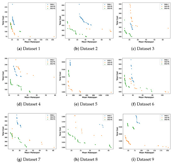
Figure 4. Pareto front obtained by three algorithms for comparison using random workflows. Axes: mean makespan (s) vs. total cost ($).

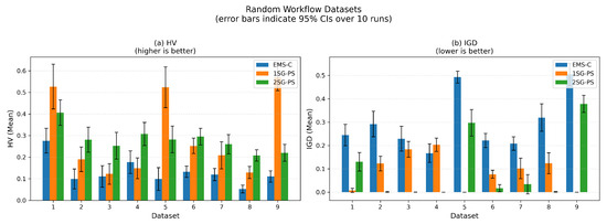
Figure 5. Bar plots of mean HV and IGD with 95% confidence intervals obtained by each algorithm on randomly generated datasets over 10 runs. Higher HV is better; lower IGD is better. The hypervolume reference point is set to $(1.1, 1.1)$ in normalized objective space. Exact mean ± std values are reported in Table 5.

From Figure 4, 2SG-PS found better solutions compared to EMS-C and 1SG-PS in most cases. For datasets 2, 3, 4, 8, the solutions found by 2SG-PS are significantly better than 1SG-PS. For datasets 1, 5, the Pareto front of 2SG-PS and 1SG-PS are overlapping, though 1SG-PS has a larger diversity of solutions. For dataset 9 (see Figure 4i), 2SG-PS found solutions that are worse compared to 1SG-PS.

From Figure 5, 2SG-PS achieves a larger HV than EMS-C, indicating more diverse solutions and larger variance in the quality of the solution compared to EMS-C. Although 2SG-PS has a lower HV compared to 1SG-PS in datasets 1, 5 and 9, it has a higher HV in the remaining datasets. Similarly, in Figure 5, it can be seen that 2SG-PS has a smaller IGD compared to EMS-C, while smaller IGD compared to 1SG-PS in most datasets. This indicates that 2SG-PS find solutions that are closer to the Pareto front compared to EMS-C.

Referring back to the dataset parameters in Table 4, we can observe that 2SG-PS performs best relative to 1SG-PS on datasets with a parallelism degree of 0.3 while performing worse on datasets with a parallelism degree of 0.05. This means that 2SG-PS is more effective for workflows with highly parallel tasks, whereas its advantage diminishes for sequential workflows. When workflows are largely sequential, scheduling offers limited room for improvement because tasks must be executed in order; consequently, performance depends more strongly on resource provisioning than scheduling. In sequential workflows, the potential for parallel execution is limited, leading to fewer opportunities for optimization through scheduling techniques. Therefore, the primary focus shifts to how resources are allocated and provisioned to ensure that the sequential tasks are executed as efficiently as possible. This involves determining the optimal number and type of resources needed to minimize execution time and maximize resource utilization. However, in the 2SG-PS approach, we reduce the search space of the first stage, which focuses on scheduling.  Although this reduction can streamline the process and improve performance for parallel workflows, it can have the unintended consequence of limiting the diversity and quality of solutions available for resource provisioning.

5.4.3. Quantitative Analysis on Random Workflows

RDI serves as a compact summary indicator that reports the relative gap of each method from the best method on the same dataset. For HV (higher is better), we define

$$\mathrm{RDI}:={\displaystyle \frac{H{V}_{\mathrm{current}}-H{V}_{\mathrm{best}}}{H{V}_{\mathrm{best}}}},$$

where $H{V}_{\mathrm{best}}=max\left(\mathrm{HV}\right)$ across methods per dataset. The best method has $\mathrm{RDI}=0$; worse methods yield negative values. We interpret gaps cautiously: if the 95% confidence intervals overlap (or if the gap is within a small tie threshold), we treat the difference as within noise rather than as a meaningful improvement. Raw IGD values are reported in the mean ± std tables for completeness.

To enable a more quantitative comparison, Table 5 reports HV and IGD values (mean ± std) over 10 runs. We also report the Relative Deviation Index (RDI) for HV mean values [34] in Table 6, which shows that 2SG-PS achieves RDI $=0$ (best) on 6 out of 9 datasets, while 1SG-PS is best on the remaining 3 datasets (1, 5, 9).

Table 5. HV and IGD values (mean ± std) on random workflow set over 10 runs. Higher HV is better; lower IGD is better.

Dataset	HV (Mean ± Std)			IGD (Mean ± Std)
	EMS-C	1SG-PS	2SG-PS	EMS-C	1SG-PS	2SG-PS
1	0.276 ± 0.076	0.527 ± 0.138	0.406 ± 0.078	0.245 ± 0.060	0.008 ± 0.012	0.130 ± 0.053
2	0.099 ± 0.061	0.190 ± 0.075	0.281 ± 0.077	0.292 ± 0.073	0.123 ± 0.041	0.001 ± 0.002
3	0.111 ± 0.066	0.122 ± 0.063	0.253 ± 0.082	0.229 ± 0.071	0.184 ± 0.044	0.000 ± 0.000
4	0.177 ± 0.069	0.149 ± 0.063	0.308 ± 0.071	0.167 ± 0.052	0.203 ± 0.038	0.000 ± 0.000
5	0.099 ± 0.070	0.524 ± 0.125	0.282 ± 0.082	0.493 ± 0.034	0.000 ± 0.000	0.297 ± 0.076
6	0.133 ± 0.035	0.252 ± 0.048	0.295 ± 0.051	0.221 ± 0.040	0.077 ± 0.022	0.017 ± 0.021
7	0.119 ± 0.037	0.209 ± 0.083	0.260 ± 0.060	0.208 ± 0.038	0.102 ± 0.058	0.034 ± 0.055
8	0.053 ± 0.023	0.129 ± 0.037	0.208 ± 0.035	0.320 ± 0.078	0.124 ± 0.059	0.001 ± 0.002
9	0.110 ± 0.035	0.570 ± 0.082	0.220 ± 0.052	0.504 ± 0.062	0.000 ± 0.000	0.378 ± 0.048

Table 6. RDI for HV mean on random workflow set. RDI $:=(H{V}_{\mathrm{current}}-H{V}_{\mathrm{best}})/H{V}_{\mathrm{best}}$, where $H{V}_{\mathrm{best}}=max\left(\mathrm{HV}\right)$ per dataset. The best method has RDI $=0$; worse methods yield negative values. Raw IGD values are reported separately in Table 5.

Datasets	EMS-C	1SG-PS	2SG-PS
1	−0.476	0	−0.230
2	−0.648	−0.324	0
3	−0.561	−0.518	0
4	−0.425	−0.516	0
5	−0.811	0	−0.462
6	−0.549	−0.146	0
7	−0.542	−0.196	0
8	−0.745	−0.380	0
9	−0.807	0	−0.614

Table 5 reports the exact mean and standard deviation of HV and IGD over 10 independent runs. To statistically validate the HV differences, Table 7 presents HV-based pairwise comparisons using Wilcoxon signed-rank tests and Cliff’s delta effect sizes. Against EMS-C, 2SG-PS achieves 9 wins out of 9 comparisons with all p-values equal to 0.002 and large effect sizes ($\delta \ge 0.78$). Against 1SG-PS, 2SG-PS wins 6 out of 9 comparisons; the 3 losses occur on datasets 1, 5, and 9 where 1SG-PS performs better, consistent with the observation that 2SG-PS is less effective on low-parallelism workflows. We note that datasets with near-zero RDI values correspond to cases where win/tie/loss counts and effect sizes indicate weak or inconsistent differences, whereas larger-magnitude RDI values align with consistent wins and larger effect sizes for 2SG-PS.

Table 7. Statistical comparison of 2SG-PS against baselines on random workflows based on per-run HV values over 10 runs. W/T/L are counted with a tie threshold $|\Delta HV|<{10}^{-3}$. p-value: Wilcoxon signed-rank test. $\delta$: Cliff’s delta effect size.

Dataset	2SG-PS vs. EMS-C					2SG-PS vs. 1SG-PS
	W	T	L	p-Value	$\mathit{\delta }$	W	T	L	p-Value	$\mathit{\delta }$
1	10	0	0	0.002	0.78	0	0	10	0.002	−0.54
2	10	0	0	0.002	0.90	10	0	0	0.002	0.62
3	10	0	0	0.002	0.84	10	0	0	0.002	0.80
4	10	0	0	0.002	0.78	10	0	0	0.002	0.88
5	10	0	0	0.002	0.90	0	0	10	0.002	−0.92
6	10	0	0	0.002	1.00	10	0	0	0.002	0.52
7	10	0	0	0.002	0.98	7	0	3	0.037	0.36
8	10	0	0	0.002	1.00	10	0	0	0.002	0.86
9	10	0	0	0.002	0.90	0	0	10	0.002	−1.00
Total	90	0	0	-	-	57	0	33	-	-

5.5. Scientific Workflows

5.5.1. Dataset Design

Pegasus project has published the workflows of many complex scientific workflow applications, including Montage, CyberShake, Epigenomics, LIGO Inspiral Analysis, and SIPHT [35,36]. For each workflow, the published details include the workflow, the sizes of data transfer, and the reference execution time based on Intel Xeon@2.33 GHz CPUs. The characteristics of these workflows, including the numbers of tasks and edges, average data size, and average task runtime, are given in Table 8, and the structures of different applications are given in Figure 6. Based on this set of workflows, we generate five datasets of varying sizes $\{10, 20, 30, 40, 50\}$. Each dataset is randomly selected from the set of scientific workflows up to the size of the dataset. In addition, we include Dataset 6 (1000Genome_52), a publicly available workflow instance from WfCommons [37], to broaden the evaluation on modern, data-intensive genomics pipelines.

Table 8. Characteristics of the scientific workflows.

Workflow	# Tasks	# Edges	Av. Data Size (MB)	Av. Task Runtime (s)
CyberShake 30	30	112	747.48	23.77
CyberShake 50	50	188	864.74	29.32
Epigenomics 24	24	75	116.20	681.54
Epigenomics 46	46	148	104.81	844.93
Epigenomics 100	100	322	395.10	3954.90
Inspiral 30	30	95	9.00	206.78
Inspiral 50	50	160	9.16	226.19
Montage 25	25	95	3.43	8.44
Montage 50	50	206	3.36	9.78
Montage 100	100	433	3.23	10.58
Sipht 30	30	91	7.73	178.92
Sipht 60	60	198	6.95	194.48

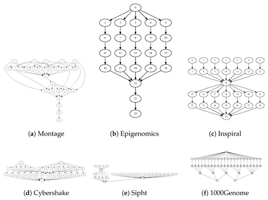
Figure 6. Structures of scientific workflows. (a) Montage, (b) Epigenomics, (c) Inspiral, (d) CyberShake, (e) Sipht, and (f) 1000Genome.

5.5.2. Experimental Results

The Pareto fronts for each dataset are presented in Figure 7, and the bar plots of HV and IGD obtained by ten runs for each algorithm on six datasets are shown in Figure 8. From the figures, it can be seen that 2SG-PS performs better than both EMS-C and 1SG-PS except dataset 5, where there is an overlap on the Pareto front of 2SG-PS and EMS-C (see Figure 7e). However, 2SG-PS has the largest HV on all datasets including dataset 5 shown in Figure 8, which means 2SG-PS performs best among all compared methods. This can also be seen in the very small IGD in Figure 8. This illustrates that the proposed algorithm can find more diverse solutions.

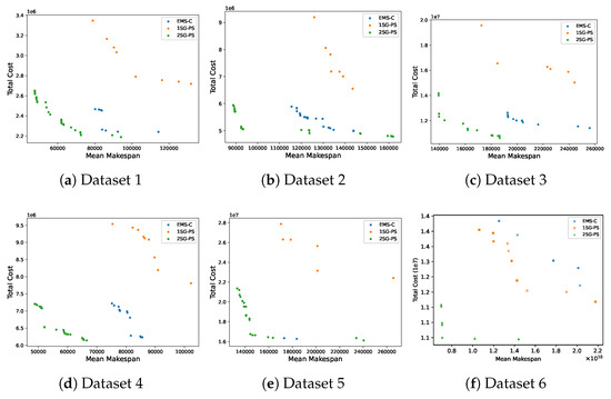
Figure 7. Pareto front obtained by three algorithms for comparison using scientific workflows. Axes: mean makespan (s) vs. total cost ($).

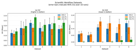
Figure 8. Bar plots of mean HV and IGD with 95% confidence intervals obtained by each algorithm on scientific workflow datasets over 10 runs. Higher HV is better; lower IGD is better. The hypervolume reference point is set to $(1.1, 1.1)$ in normalized objective space. Exact mean ± std values are reported in Table 9.

As seen in the structures of the scientific workflows in Figure 6, these workflows usually contain a large number of parallel tasks. The main purpose of utilizing workflows to run applications is to leverage large computing resources to execute parallel tasks. Therefore, 2SG-PS is effective in allocating suitable resources and finding an optimal schedule for these workflows.

1SG-PS optimizes the resource pool and scheduling concurrently, where both optimizations are interdependent. Therefore, it may hinder convergence, as changing the resource pool may cause the scheduling to be no longer optimized. This is observed in the large gap in the Pareto fronts between 1SG-PS and 2SG-PS in Figure 7. On the other hand, instead of directly optimizing resource provisioning, EMS-C optimizes the instance and resource types to execute tasks, and the number of resource instances is only established based on the instance and type. EMS-C uses a co-evolutionary approach in the crossover operation, i.e., the same crossover point is used for resource instance and type. This limits the diversity of solutions for EMS-C, as seen in Figure 8.

5.5.3. Quantitative Analysis

Table 9 reports the HV and IGD values (mean ± std) on scientific workflows. 2SG-PS achieves the highest HV and lowest IGD across all six datasets. Table 10 shows the HV-based RDI results, where 2SG-PS achieves RDI $=0$ (best HV) on all datasets, confirming its consistent superiority. When RDI differences fall within the reported variability (e.g., overlapping confidence intervals in Figure 8), we do not interpret them as statistically meaningful.

Table 9. HV and IGD values (mean ± std) on scientific workflow set over 10 runs. Higher HV is better; lower IGD is better.

Dataset	HV (Mean ± Std)			IGD (Mean ± Std)
	EMS-C	1SG-PS	2SG-PS	EMS-C	1SG-PS	2SG-PS
1	0.125 ± 0.040	0.117 ± 0.040	0.141 ± 0.040	0.059 ± 0.029	0.065 ± 0.022	0.003 ± 0.007
2	0.176 ± 0.091	0.171 ± 0.088	0.196 ± 0.086	0.051 ± 0.030	0.057 ± 0.021	0.001 ± 0.004
3	0.227 ± 0.036	0.178 ± 0.049	0.283 ± 0.034	0.109 ± 0.028	0.154 ± 0.040	0.001 ± 0.002
4	0.176 ± 0.073	0.142 ± 0.065	0.207 ± 0.070	0.099 ± 0.048	0.141 ± 0.072	0.003 ± 0.006
5	0.214 ± 0.082	0.166 ± 0.078	0.223 ± 0.090	0.068 ± 0.054	0.134 ± 0.049	0.013 ± 0.037
6	0.165 ± 0.048	0.170 ± 0.036	0.229 ± 0.040	0.142 ± 0.083	0.110 ± 0.062	0.017 ± 0.024

Table 10. RDI for HV mean on scientific workflow set. RDI $:=(H{V}_{\mathrm{current}}-H{V}_{\mathrm{best}})/H{V}_{\mathrm{best}}$, where $H{V}_{\mathrm{best}}=max\left(\mathrm{HV}\right)$ per dataset. The best method has RDI $=0$; worse methods yield negative values. Raw IGD values are reported separately in Table 9.

Datasets	EMS-C	1SG-PS	2SG-PS
1	−0.113	−0.170	0
2	−0.102	−0.128	0
3	−0.198	−0.371	0
4	−0.150	−0.314	0
5	−0.040	−0.256	0
6	−0.279	−0.258	0

Table 9 reports the exact mean and standard deviation of HV and IGD over 10 independent runs. The results show that 2SG-PS consistently achieves the highest HV and lowest IGD across all six scientific workflow datasets. To statistically validate the HV differences, Table 11 presents HV-based pairwise comparisons using Wilcoxon signed-rank tests and Cliff’s delta effect sizes. Against EMS-C, 2SG-PS achieves 6 wins out of 6 comparisons with all p-values below 0.05. Against 1SG-PS, 2SG-PS wins all 6 comparisons, demonstrating statistically significant and consistent superiority on scientific workflows.

Table 11. Statistical comparison of 2SG-PS against baselines on scientific workflows based on per-run HV values over 10 runs. W/T/L are counted with a tie threshold $|\Delta HV|<{10}^{-3}$. p-value: Wilcoxon signed-rank test. $\delta$: Cliff’s delta effect size.

Dataset	2SG-PS vs. EMS-C					2SG-PS vs. 1SG-PS
	W	T	L	p-Value	$\mathit{\delta }$	W	T	L	p-Value	$\mathit{\delta }$
1	10	0	0	0.002	0.28	10	0	0	0.002	0.36
2	10	0	0	0.002	0.22	10	0	0	0.002	0.28
3	10	0	0	0.002	0.70	10	0	0	0.002	0.94
4	8	0	2	0.014	0.20	10	0	0	0.002	0.52
5	8	0	2	0.010	0.10	10	0	0	0.002	0.42
6	10	0	0	0.002	0.72	10	0	0	0.002	0.82
Total	56	0	4	-	-	60	0	0	-	-

To provide a single representative solution from each Pareto front, we report the utopia-based knee point for each algorithm. For each algorithm and dataset, we performed 10 independent runs and extracted a knee solution from the final Pareto set in each run. Table 12 reports the mean knee makespan and cost across runs.

Table 12. Knee-point (utopia-based) solutions on the scientific workflow sets.

Dataset	Workflow	Knee Makespan (s)			Knee Cost
		EMS-C	1SG-PS	2SG-PS	EMS-C	1SG-PS	2SG-PS
1	CyberShake 50	$1.440\times {10}^3$	$1.386\times {10}^3$	$1.405\times {10}^3$	$5.115\times {10}^3$	$5.311\times {10}^3$	$4.993\times {10}^3$
2	Epigenomics 46	$4.879\times {10}^4$	$4.749\times {10}^4$	$4.166\times {10}^4$	$1.568\times {10}^5$	$1.618\times {10}^5$	$1.559\times {10}^5$
3	Inspiral 50	$1.257\times {10}^4$	$1.396\times {10}^4$	$1.134\times {10}^4$	$4.850\times {10}^4$	$5.233\times {10}^4$	$4.490\times {10}^4$
4	Epigenomics 100	$2.854\times {10}^5$	$3.575\times {10}^5$	$2.326\times {10}^5$	$1.527\times {10}^6$	$1.620\times {10}^6$	$1.517\times {10}^6$
5	Sipht 60	$1.983\times {10}^4$	$2.270\times {10}^4$	$1.961\times {10}^4$	$4.598\times {10}^4$	$5.145\times {10}^4$	$4.377\times {10}^4$
6	1000Genome 52	$3.075\times {10}^6$	$2.890\times {10}^6$	$1.925\times {10}^6$	$1.080\times {10}^7$	$1.120\times {10}^7$	$1.055\times {10}^7$

To illustrate the search dynamics and convergence behavior on real workflow applications, Figure 9 presents the HV convergence curves over generations for two representative scientific workflow datasets (Sipht_60 and 1000Genome_52). The results show that 2SG-PS achieves rapid early improvement and maintains a stable HV plateau in later generations, benefiting from the two-stage decomposition and caching of intermediate results.

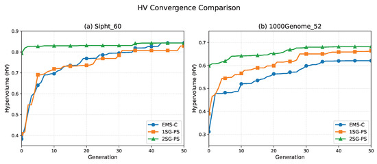
Figure 9. Convergence curves of HV over generations on Sipht_60 (a) and 1000Genome_52 (b).

5.6. Robustness Analysis

We further evaluated robustness to the instance-budget setting by varying the total instance budget $\overline{R}$ by $\pm 20\%$ while keeping the equal per-type split rule unchanged. Table 13 reports HV (final archive mean) under these budget variations, together with convergence indicators measured at $1.0\overline{R}$: runtime (wall-clock seconds), Gen@HV* (first generation reaching the fixed threshold), and SR (success rate).

Table 13. Budget sensitivity and convergence speed under global normalization (HV ref=$(1.1, 1.1)$). HV reports the final archive HV averaged over runs (higher is better). Runtime is the mean wall-clock time of a full 50-generation run at $1.0\overline{R}$. Gen@HV* is the first generation reaching the dataset-wise fixed threshold $H{V}^{\ast }\left(d\right)=0.95·{max}_{m\in \mathcal{M}}{\widetilde{HV}}_{\mathrm{final}}^{\left(m\right)}\left(d\right)$, where ${\widetilde{HV}}_{\mathrm{final}}^{\left(m\right)}\left(d\right)$ is the median final HV of method m over runs. We obtain $H{V}^{\ast }=0.7938$ for Sipht_60 and $H{V}^{\ast }=0.6308$ for 1000Genome_52. Gen@HV* is reported as median [min–max] over successful runs; SR denotes success rate (%).

Dataset	Algo	HV (Final Mean) ↑			At $1.0\overline{\mathit{R}}$ (G = 50)
		$\mathbf{0}.\mathbf{8}\overline{\mathbf{R}}$	$\mathbf{1}.\mathbf{0}\overline{\mathbf{R}}$	$\mathbf{1}.\mathbf{2}\overline{\mathbf{R}}$	Runtime (s)	Gen@HV*	SR
Sipht_60	EMS-C	0.823	0.832	0.840	1.5	35 [31–38]	100%
	1SG-PS	0.797	0.806	0.814	1.1	48 [44–48]	43%
	2SG-PS	0.838	0.845	0.848	78.0	6 [4–8]	100%
1000Genome_52	EMS-C	0.579	0.610	0.610	1.0	47	14%
	1SG-PS	0.602	0.610	0.614	0.9	21	14%
	2SG-PS	0.670	0.674	0.660	55.7	13 [12–16]	100%

Under all three budget levels ($0.8\overline{R}$, $1.0\overline{R}$, $1.2\overline{R}$), the relative ranking of methods remains stable, confirming that the conclusions do not hinge on a single budget choice. Regarding convergence speed, 2SG-PS reaches the target HV level in fewer generations than EMS-C on most datasets, demonstrating efficient early-stage improvement from the two-stage decomposition and caching strategy.

6. Conclusions and Future Work

To address the multi-objective problem of resource provisioning and scheduling, we propose a two-stage genetic-based optimization algorithm considering resource constraints. The first stage optimizes a candidate resource pool, while the second stage optimizes resource provisioning and task scheduling. The first-stage solutions are not evaluated directly in the first stage; they are used to generate the resource instances in the resource pool, which serves as the basis for schedule optimization in the second stage. A new ranking and selection procedure is proposed in the first stage, where the new generation is selected by combining the Pareto solutions from the second stage. To reduce the search space, the first stage utilizes a smaller population size and runs for fewer generations. The intermediate optimization results for the second stage can also be cached to reduce the number of required evaluations.

Experiments demonstrate the effectiveness of the proposed algorithm by comparing it with resource provisioning and scheduling algorithms, 1SG-PS and EMS-C, under the same NSGA-II framework using IGD and HV. Both randomly generated and scientific workflows are used as datasets for comparison. Our proposed algorithm demonstrates more diverse and higher-quality solutions than the two compared methods, especially for workflows with high parallelisms. The key benefit of a two-stage optimization approach is its improved convergence stability of resource provisioning and task scheduling, albeit at the cost of more evaluations.

The superiority of 2SG-PS can be explained by its two-stage structure, which reduces the coupling between provisioning and scheduling decisions under the same VM-instance constraints. Stage 1 determines a cost-effective and feasible resource pool under $|R_m|\le {\overline{R}}_m$ and $\left|P\right|\le \overline{R}$, while Stage 2 refines scheduling decisions on this fixed pool, enabling more effective exploration of cost–makespan trade-offs. This staged design is consistent with the reported set-level improvements (higher HV and lower IGD) and the improved representative knee-point trade-offs in Section 5, compared with 1SG-PS (without staged decomposition) and EMS-C.

Although the proposed two-stage GA improves solution quality, it incurs additional overhead mainly due to repeated fitness evaluations across generations and the cost of schedule evaluation under precedence constraints. Moreover, the current model assumes static VM provisioning within a planning horizon and does not consider dynamic scaling or migration. These limitations indicate that further runtime optimization (e.g., parallel fitness evaluation) and extensions to elastic environments are important future work. In the future, research can focus on methods to reduce the search space and optimize algorithm parameters. Additionally, exploring various combinations of task ordering methods for multiple workflows and different resource provisioning algorithms could be beneficial. In addition, a more accurate model that includes the initial boot time of each instance should be considered.

References

- Li, X.; Cai, Z. Elastic resource provisioning for cloud workflow applications. IEEE Trans. Autom. Sci. Eng. 2015, 14, 1195–1210. [Google Scholar] [CrossRef]
- Taylor, I.J.; Deelman, E.; Gannon, D.B.; Shields, M. (Eds.) Workflows for e-Science: Scientific Workflows for Grids; Springer: London, UK, 2007; Volume 1. [Google Scholar]
- Rodriguez, M.A.; Buyya, R. Scheduling dynamic workloads in multi-tenant scientific workflow as a service platforms. Future Gener. Comput. Syst. 2018, 79, 739–750. [Google Scholar] [CrossRef]
- Mboula, J.E.N.; Kamla, V.C.; Djamegni, C.T. Cost-time trade-off efficient workflow scheduling in cloud. Simul. Model. Pract. Theory 2020, 103, 102107. [Google Scholar] [CrossRef]
- Cai, Z.; Li, Q.; Li, X. Elasticsim: A toolkit for simulating workflows with cloud resource runtime auto-scaling and stochastic task execution times. J. Grid Comput. 2017, 15, 257–272. [Google Scholar] [CrossRef]
- Anwar, N.; Deng, H. A hybrid metaheuristic for multi-objective scientific workflow scheduling in a cloud environment. Appl. Sci. 2018, 8, 538. [Google Scholar] [CrossRef]
- Chen, Z.G.; Zhan, Z.H.; Lin, Y.; Gong, Y.J.; Gu, T.L.; Zhao, F.; Yuan, H.Q.; Chen, X.; Li, Q.; Zhang, J. Multiobjective cloud workflow scheduling: A multiple populations ant colony system approach. IEEE Trans. Cybern. 2018, 49, 2912–2926. [Google Scholar] [CrossRef] [PubMed]
- Byun, E.K.; Kee, Y.S.; Kim, J.S.; Maeng, S. Cost optimized provisioning of elastic resources for application workflows. Future Gener. Comput. Syst. 2011, 27, 1011–1026. [Google Scholar] [CrossRef]
- Abrishami, S.; Naghibzadeh, M.; Epema, D.H. Deadline-constrained workflow scheduling algorithms for infrastructure as a service clouds. Future Gener. Comput. Syst. 2013, 29, 158–169. [Google Scholar] [CrossRef]
- Topcuoglu, H.; Hariri, S.; Wu, M.Y. Performance-effective and low-complexity task scheduling for heterogeneous computing. IEEE Trans. Parallel Distrib. Syst. 2002, 13, 260–274. [Google Scholar] [CrossRef]
- Chen, W.N.; Zhang, J. An ant colony optimization approach to a grid workflow scheduling problem with various QoS requirements. IEEE Trans. Syst. Man Cybern. Part C (Appl. Rev.) 2008, 39, 29–43. [Google Scholar] [CrossRef]
- Li, F.; Liao, T.W.; Cai, W. Research on the collaboration of service selection and resource scheduling for IoT simulation workflows. Adv. Eng. Inform. 2022, 52, 101528. [Google Scholar] [CrossRef]
- Xia, X.; Qiu, H.; Xu, X.; Zhang, Y. Multi-objective workflow scheduling based on genetic algorithm in cloud environment. Inf. Sci. 2022, 606, 38–59. [Google Scholar] [CrossRef]
- Kumar, M.; Sharma, S.C.; Goel, S.; Mishra, S.K.; Husain, A. Autonomic cloud resource provisioning and scheduling using meta-heuristic algorithm. Neural Comput. Appl. 2020, 32, 18285–18303. [Google Scholar] [CrossRef]
- Ghobaei-Arani, M.; Shahidinejad, A. An efficient resource provisioning approach for analyzing cloud workloads: A metaheuristic-based clustering approach. J. Supercomput. 2021, 77, 711–750. [Google Scholar] [CrossRef]
- Mao, M.; Li, J.; Humphrey, M. Cloud auto-scaling with deadline and budget constraints. In Proceedings of the 2010 11th IEEE/ACM International Conference on Grid Computing, Brussels, Belgium, 25–29 October 2010; IEEE: Piscataway, NJ, USA, 2010; pp. 41–48. [Google Scholar]
- Bi, J.; Yuan, H.; Tan, W.; Zhou, M.; Fan, Y.; Zhang, J.; Li, J. Application-aware dynamic fine-grained resource provisioning in a virtualized cloud data center. IEEE Trans. Autom. Sci. Eng. 2015, 14, 1172–1184. [Google Scholar] [CrossRef]
- Arabnejad, V.; Bubendorfer, K.; Ng, B. Budget and deadline aware e-science workflow scheduling in clouds. IEEE Trans. Parallel Distrib. Syst. 2018, 30, 29–44. [Google Scholar] [CrossRef]
- Faragardi, H.R.; Sedghpour, M.R.S.; Fazliahmadi, S.; Fahringer, T.; Rasouli, N. GRP-HEFT: A budget-constrained resource provisioning scheme for workflow scheduling in IaaS clouds. IEEE Trans. Parallel Distrib. Syst. 2019, 31, 1239–1254. [Google Scholar] [CrossRef]
- Garg, N.; Singh, D.; Goraya, M.S. Energy and resource efficient workflow scheduling in a virtualized cloud environment. Clust. Comput. 2021, 24, 767–797. [Google Scholar] [CrossRef]
- Rajasekar, P.; Palanichamy, Y. Adaptive resource provisioning and scheduling algorithm for scientific workflows on IaaS cloud. SN Comput. Sci. 2021, 2, 456. [Google Scholar] [CrossRef]
- Rodriguez, M.A.; Buyya, R. Deadline based resource provisioning and scheduling algorithm for scientific workflows on clouds. IEEE Trans. Cloud Comput. 2014, 2, 222–235. [Google Scholar] [CrossRef]
- Zhu, Z.; Zhang, G.; Li, M.; Liu, X. Evolutionary multi-objective workflow scheduling in cloud. IEEE Trans. Parallel Distrib. Syst. 2015, 27, 1344–1357. [Google Scholar] [CrossRef]
- Malawski, M.; Juve, G.; Deelman, E.; Nabrzyski, J. Algorithms for cost-and deadline-constrained provisioning for scientific workflow ensembles in IaaS clouds. Future Gener. Comput. Syst. 2015, 48, 1–18. [Google Scholar] [CrossRef]
- Shishido, H.Y.; Estrella, J.C.; Toledo, C.F.M.; Arantes, M.S. Genetic-based algorithms applied to a workflow scheduling algorithm with security and deadline constraints in clouds. Comput. Electr. Eng. 2018, 69, 378–394. [Google Scholar] [CrossRef]
- Khan, M.A.; Rasool, R.u. A multi-objective grey-wolf optimization based approach for scheduling on cloud platforms. J. Parallel Distrib. Comput. 2024, 187, 104847. [Google Scholar] [CrossRef]
- Rathi, S.; Nagpal, R.; Srivastava, G.; Mehrotra, D. A multi-objective fitness dependent optimizer for workflow scheduling. Appl. Soft Comput. 2024, 152, 111247. [Google Scholar] [CrossRef]
- Cai, X.; Zhang, Y.; Li, M.; Wu, L.; Zhang, W.; Chen, J. Dynamic deadline constrained multi-objective workflow scheduling in multi-cloud environments. Expert Syst. Appl. 2024, 258, 125168. [Google Scholar] [CrossRef]
- Mikram, H.; El Kafhali, S.; Saadi, Y. HEPGA: A new effective hybrid algorithm for scientific workflow scheduling in cloud computing environment. Simul. Model. Pract. Theory 2024, 130, 102864. [Google Scholar] [CrossRef]
- Rimal, B.P.; Maier, M. Workflow scheduling in multi-tenant cloud computing environments. IEEE Trans. Parallel Distrib. Syst. 2016, 28, 290–304. [Google Scholar] [CrossRef]
- Ishibuchi, H.; Hitotsuyanagi, Y.; Tsukamoto, N.; Nojima, Y. Many-objective test problems to visually examine the behavior of multiobjective evolution in a decision space. In Proceedings of the International Conference on Parallel Problem Solving from Nature, Kraków, Poland, 11–15 September 2010; Springer: Berlin/Heidelberg, Germany, 2010; pp. 91–100. [Google Scholar]
- Zitzler, E.; Thiele, L.; Laumanns, M.; Fonseca, C.M.; Da Fonseca, V.G. Performance assessment of multiobjective optimizers: An analysis and review. IEEE Trans. Evol. Comput. 2003, 7, 117–132. [Google Scholar] [CrossRef]
- Li, F.; Seok, M.G.; Cai, W. A New Double Rank-based Multi-workflow Scheduling with Multi-objective Optimization in Cloud Environments. In Proceedings of the 2021 IEEE International Parallel and Distributed Processing Symposium Workshops (IPDPSW), Portland, OR, USA, 17–21 June 2021; IEEE: Piscataway, NJ, USA, 2021; pp. 36–45. [Google Scholar]
- Li, F.; Jun, W. Multi-objective optimization of clustering-based scheduling for multi-workflow on clouds considering fairness. arXiv 2022, arXiv:2205.11173. [Google Scholar] [CrossRef]
- Bharathi, S.; Chervenak, A.; Deelman, E.; Mehta, G.; Su, M.H.; Vahi, K. Characterization of scientific workflows. In Proceedings of the 2008 THIRD workshop on Workflows in Support of Large-Scale Science, Austin, TX, USA, 17 November 2008; IEEE: Piscataway, NJ, USA, 2008; pp. 1–10. [Google Scholar]
- Juve, G.; Chervenak, A.; Deelman, E.; Bharathi, S.; Mehta, G.; Vahi, K. Characterizing and profiling scientific workflows. Future Gener. Comput. Syst. 2013, 29, 682–692. [Google Scholar]
- Coleman, T.; Casanova, H.; Pottier, L.; Kaushik, M.; Deelman, E.; Ferreira da Silva, R. WfCommons: A Framework for Enabling Scientific Workflow Research and Development. Future Gener. Comput. Syst. 2022, 128, 16–27. [Google Scholar] [CrossRef]
Disclaimer/Publisher’s Note: The statements, opinions and data contained in all publications are solely those of the individual author(s) and contributor(s) and not of MDPI and/or the editor(s). MDPI and/or the editor(s) disclaim responsibility for any injury to people or property resulting from any ideas, methods, instructions or products referred to in the content. |
© 2026 by the authors. Licensee MDPI, Basel, Switzerland. This article is an open access article distributed under the terms and conditions of the Creative Commons Attribution (CC BY) license.