Article

Data-Dependent Weighted E-Value Aggregation for Fusion Learning

1
Department of Statistics, Beijing Normal University at Zhuhai, Zhuhai 519087, China
2
Guangdong Provincial/Zhuhai Key Laboratory of Interdisciplinary Research and Application for Data Science, Beijing Normal-Hong Kong Baptist University, Zhuhai 519087, China
*
Author to whom correspondence should be addressed.
Mathematics 2026, 14(1), 88; https://doi.org/10.3390/math14010088
Submission received: 1 December 2025 / Revised: 20 December 2025 / Accepted: 21 December 2025 / Published: 26 December 2025
(This article belongs to the Special Issue Computational Statistics and Data Analysis, 3rd Edition)

Abstract

We propose a data-dependent weighted e-value aggregation framework for synthesizing discoveries across partially overlapping studies. The key idea is to convert within study p-value-based multiple testing results into e-values and aggregate them using data-dependent leave-one-out weights, thereby mitigating the power loss associated with naive averaging. We show that applying the e-Benjamini–Hochberg procedure to the aggregated e-values yields finite-sample control of the global false discovery rate under standard conditions. Simulation studies and real-data analyses demonstrate the effectiveness and practical advantages of the proposed methods.

1. Introduction

In modern applications with high dimensional data, investigators routinely test many hypotheses simultaneously to detect signals. This multiplicity requires rigorous control of error rates, especially the false discovery rate (FDR) [1], to ensure valid statistical inference.
The Benjamini–Hochberg (BH) procedure [1] is the most widely used method for FDR control. Recently, Barber and Candes [2] introduced the Barber–Candès (BC) procedure, which estimates the number of false discoveries by exploiting the symmetry of null p-values and achieves FDR control under suitable independence conditions. In the recent literature, a growing line of work advocates e-values as convenient tools for multiple testing. An e-value is a non-negative random variable e 0 with expectation at most one under the null hypothesis. There is increasing interest in using e-values to control the FDR in both offline and online settings [3,4,5]. In particular, Wang and Ramdas [6] proposed the e–Benjamini–Hochberg (e-BH) procedure, which applies the BH rule to the inverses of e-values, and proved that it controls the FDR under arbitrary dependence among e-values. Recent work by Li and Zhang [7] establishes an equivalence between several p-value-based methods (including BH and BC) and e-BH when appropriate e-values are constructed; equivalence here means the procedures yield identical rejection sets.
In this paper, we consider J studies that test overlapping subsets of a total of m hypotheses. Study j tests m j hypotheses, where m j m . This partial-overlap regime arises naturally in fusion learning from multiple data sources and has been studied in recent work [8,9,10]. Examples include multicenter clinical trials [11], multicohort genomics [12,13], and federated A/B testing [14]. The goal is to synthesize evidence across studies into a unified set of discoveries while controlling the global FDR.
Principled aggregation is motivated by practical constraints. Studies often examine different subsets of hypotheses, vary in sample size and signal strength, and face data sharing restrictions that provide only summary statistics such as vectors of p-values. Naive aggregation of study specific findings performs poorly in practice. For example, taking the intersection of rejection sets is typically too conservative, whereas taking their union can inflate the global FDR because error control within each study does not automatically imply control of the overall FDR.
Since p-values are the most widely used quantities in multiple testing, we assume that each study applies a p-value-based procedure. Direct aggregation of p-values is difficult, so motivated by Li and Zhang [7], we map each study’s results to e-values and then aggregate across studies using e-values. However, how to combine e-values across studies is a central design choice. A common approach is simple averaging [15], which underlies several recent aggregation methods [7,16]. Ren and Barber [16] propose derandomized knockoffs that aggregate via averaged e-values, while Banerjee et al. [9] introduce an Integrative Ranking and Thresholding (IRT) framework that aggregates only binary decisions. However, our simulations show that naive averaging can substantially reduce power. Motivated by Li and Zhang [17], we adapt leave-one-out (LOO) ideas to construct data-dependent weights for combining e-values across studies. These weights enhance power while preserving global FDR control.
In this work, we propose two e-value-based fusion methods tailored to overlapping studies. The first, BH-based fusion, runs BH within each study, maps its outputs to e-values, combines these e-values across studies using data-dependent weights, and then applies e-BH globally. The second, BC-based fusion, runs BC within each study and proceeds analogously. Our main theoretical results establish finite-sample FDR control for e-BH applied to the aggregated e-values produced by our weighting schemes.
The remainder of the paper is organized as follows. Section 2 reviews preliminaries on FDR, multiple testing procedures, and e-values. Section 3 presents our data-dependent weighted e-value aggregation method for fusion learning. Section 4 reports simulation results, and Section 5 illustrates the method on real data. Section 6 concludes. All proofs and additional numerical results are deferred to the Appendixes Appendix A and  Appendix B.

2. Preliminaries

2.1. Basic Setup and False Discovery Rate

Consider m hypotheses M : = { H 1 , , H m } , indexed by [ m ] : = { 1 , , m } . Let θ = ( θ 1 , , θ m ) { 0 , 1 } m denote the ground truth, where θ i = 0 if H i is a true null and θ i = 1 otherwise. Define the index sets of true nulls and non-nulls as H 0 : = { i [ m ] : θ i = 0 } and H 1 : = { i [ m ] : θ i = 1 } , respectively. A decision rule is a vector δ = ( δ 1 , , δ m ) { 0 , 1 } m , where δ i = 1 indicates rejection of H i and δ i = 0 indicates non-rejection. Throughout, “non-null” and “under the alternative” are used interchangeably.
The false discovery rate (FDR) associated with a decision rule δ is defined as the expectation of the false discovery proportion (FDP):
FDR ( δ ) = E FDP ( δ ) , where FDP ( δ ) = i = 1 m ( 1 θ i ) δ i 1 i = 1 m δ i ,
with a b max { a , b } . The convention 1 i = 1 m δ i prevents division by zero when no hypotheses are rejected. An FDR-controlling procedure guarantees that FDR ( δ ) α for a pre-specified level α ( 0 , 1 ) .
We consider a multi-study setting in which the m hypotheses in M are tested across J studies. Study j tests a subset M j M with index set I j [ m ] , so that M j = { H i : i I j } . Let m j | I j | ; studies may overlap, hence j = 1 J M j = M and j = 1 J m j m . For each hypothesis i, let N i [ J ] denote the set of study indices that test H i : N i = { j [ J ] : i I j } , and  n i | N i | .
For i I j , let δ j , i { 0 , 1 } denote study j’s decision for H i , with  δ j , i = 1 indicating rejection. The results of study j are collected in the decision vector δ j ( δ j , i ) i I j { 0 , 1 } m j . For study j, the false discovery rate is defined as
FDR ( δ j ) = E FDP ( δ j ) , where FDP ( δ j ) = i I j ( 1 θ i ) δ j , i 1 i I j δ j , i .
For each study j, let α j ( 0 , 1 ) be the pre-specified FDR level for which the guarantee FDR ( δ j ) α j holds. Our objective is to synthesize the evidence from all J studies to produce a combined set of rejections for the hypotheses in M , while controlling the overall FDR at a user-specified level α .

2.2. Multiple Testing Procedures

Suppose we observe m p-values p 1 , p 2 , , p m corresponding to the hypotheses H 1 , H 2 , , H m . Li and Zhang [7] showed that several widely used multiple-testing procedures can be expressed in the following unified form. Define
T = sup t T : S ( t ) 1 i = 1 m R i ( t ) α ,
where T is the admissible threshold domain, S ( t ) is a conservative estimator of the number of false rejections at threshold t, and  R i ( t ) indicates whether hypothesis H i should be rejected at threshold t. The rule selects the largest threshold T such that the estimated FDP doesn’t exceed target FDR level α .
To instantiate an FDR-controlling procedure within this framework, one specifies S ( t ) and R i ( t ) . The classical Benjamini–Hochberg (BH) procedure [1] uses
S ( t ) = m t , R i ( t ) = 1 { p i t } ,
which yields FDR α under independence or certain positive dependence conditions of p-values. The Barber–Candès (BC) procedure [2], a model-free approach that exploits the symmetry of null p-values, sets
S ( t ) = 1 + i = 1 m 1 { p i 1 t } , R i ( t ) = 1 { p i t } .
Both procedures fit into (1) by pairing a data-driven, conservative estimate S ( t ) of false discoveries with the candidate rejection set { i : R i ( t ) = 1 } and then selecting the largest threshold t for which the estimated FDP does not exceed α .

2.3. E-Values, E-BH and Equivalence to Multiple Testing Procedures

A non-negative random variable e is called an e-value if, under the null hypothesis, it satisfies E [ e ] 1 . Suppose we observe m e-values e 1 , e 2 , , e m corresponding to hypotheses H 1 , H 2 , , H m . The  α -level e–Benjamini–Hochberg (e-BH) procedure [6] proceeds by sorting the e-values in decreasing order, e ( 1 ) e ( 2 ) e ( m ) , and rejecting the hypotheses associated with the k ^ largest e-values, where
k ^ : = max i { 1 , , m } : e ( i ) m i α .
A key advantage of e-BH, established in Theorem 2 of Wang and Ramdas [6], is that it controls the FDR at level α under arbitrary dependence among the e-values, provided the following condition holds.
Proposition 1
(Wang and Ramdas [6], Theorem 2). Suppose the e-values { e i } i = 1 m satisfy
i H 0 E [ e i ] m .
Then the e-BH procedure controls the FDR at level α.
In multiple testing applications, the requirement E [ e ] 1 under the null in the definition of e-values can be relaxed. Throughout this paper, we will refer to { e i } i = 1 m as a set of e-values whenever they satisfy Condition (2).
Given the threshold T in (1), define e-values by e i = m R i ( T ) / S ( T ) for 1 i m . Then, applying the e-BH procedure to { e i } i = 1 m is equivalent to the original multiple-testing procedure based on the same functions S ( · ) and R i ( · ) [7]. Here, equivalence means that both methods produce exactly the same set of rejections.

3. Data-Dependent Weighted E-Value Aggregation for Fusion Learning

In this paper, leveraging the equivalence between e-BH and other multiple-testing procedures, we use e-values as a bridge to synthesize evidence across all J studies and to construct a combined rejection set while controlling the overall FDR at a user-specified level α .
Let e j , i denote the e-value for the ith hypothesis in the jth study. We define the combined e-value for the ith hypothesis as
e i = j N i w j , i e j , i ,
where w j , i 0 are combination weights. A simple choice is w j , i = 1 / n i , in which case e i is the average of the individual e-values across studies that test hypothesis i. It is well known that the average of e-values is again an e-value [15], and averaging is widely used to combine e-values across studies. For example, Ren and Barber [16] use this idea proposing the derandomized knockoff method, Li and Zhang [7] propose averaging e-values to combine results, and Banerjee et al. [9] adopt averaging in fusion learning. However, our simulations indicate that such a naive aggregation can reduce power. Motivated by Li and Zhang [17], we therefore propose to use data-dependent weights to aggregate e-values in the fusion-learning setting, with the goal of improving power while maintaining FDR control. The data-dependent weights are constructed using a leave-one-out analysis, a key technical tool used to establish FDR control for the BH and BC procedures [1,18].

3.1. Fusion Learning Based on the BH Procedure

Let p j = ( p j , 1 , , p j , m j ) denote the vector of p-values from the jth study, and let T j be the BH rejection threshold in that study. Following Li and Zhang [7], define the e-value for the ith hypothesis in the jth study by
e j , i = 1 T j 1 { p j , i T j } , i M j .
With these e-values, the e-BH procedure at the same target level reproduces the BH rejection set in the jth study.
To construct data-dependent weights, let p j , i be the vector obtained from p j by setting its ith entry to 0. Viewing the BH threshold as a function of p j , let T j , i denote the threshold obtained by applying BH to p j , i . Define the data-dependent weights by
w j , i = 0 , j N i , T j , i T j , i + l j , l N i T l , i , j N i .
Following the discussion in Li and Zhang [17], to make more rejections, we should assign larger weights to e-values associated with relatively large leave-one-out thresholds. Consequently, the weight w j , i is designed to increase when the leave-one-out threshold T j , i is large relative to the corresponding thresholds from other studies.
The following theorem establishes finite-sample FDR control for the e-BH procedure applied to the combined e-values in (3) with data-dependent weights in (4).
Theorem 1.
In each study, suppose the null p-values are mutually independent, satisfy super-uniformity, and are independent of the nonnull p-values. Then the e-values defined in (3) with weights given by (4) satisfy Condition (2). Consequently, the corresponding e-BH procedure controls the overall FDR in finite samples.
Proof. 
See in the Appendix A.    □
Although our data-dependent weighting scheme is inspired by Li and Zhang [17], our setting differs from theirs. Whereas Li and Zhang [17] focus on combining outputs from different testing methods, we aggregate e-values across multiple studies. Specifically, Li and Zhang [17] study multi-procedure aggregation within a single study: multiple procedures (or tuning choices) are applied to the same vector of p-values and their e-values are combined. In contrast, we consider multi-study aggregation: a fixed procedure is applied across distinct studies, each providing its own study specific vector of p-values, with heterogeneity in sample size and signal strength. Consequently, unlike the equal length, perfectly aligned e-value vectors in the multi-procedure setting, the e-value vectors we aggregate across studies can differ in length and index sets because different studies test different subsets of hypotheses. This lack of alignment induces missingness and indexing issues that complicate aggregation and motivate our study level weighting and combination rules designed to remain valid under such heterogeneity.

3.2. Fusion Learning Based on the BC Procedure

Besides the BH procedure, another well-known method is the BC procedure [2], which exploits symmetry to estimate the FDR. Let p j = ( p j , 1 , , p j , m j ) denote the vector of p-values from the jth study, and, with a slight abuse of notation, let T j be the BC rejection threshold in that study. In practice, we assume that all studies use the same multiple-testing procedure, so this notation is unambiguous regardless of the method employed. Following Li and Zhang [7], Ren and Barber [16], define the e-value for the ith hypothesis in the jth study by
e j , i = m j 1 { p j , i T j } 1 + l = 1 m j 1 { p j , l 1 T j } .
With these e-values, the e-BH procedure at the same target level reproduces the BC rejection set in the jth study.
To define data-dependent weights under the BC framework, we adopt the following convention (with a slight abuse of notation) for this section: let p j , i be the same vector as p j , except that its ith element is replaced by min { p j , i , 1 p j , i } . Viewing the BC threshold T j as a function of p j , let T j , i denote the threshold obtained by applying the BC procedure to p j , i . The data-dependent weights are then defined as
w j , i = 0 , j N i , m m j 1 + l M j , l i 1 { p j , l 1 T j } 1 + l M j , l i 1 { p j , l 1 T j } + s j l M s 1 { p s , l 1 T s , l } , j N i .
For J = 2 and all studies test m hypotheses, the weights simplify to
w 1 , i = 1 + l i 1 { p 1 , l 1 T 1 } 1 + l i 1 { p 1 , l 1 T 1 } + l = 1 m 1 { p 2 , l 1 T 2 , l } , w 2 , i = 1 + l i 1 { p 2 , l 1 T 2 } l = 1 m 1 { p 1 , l 1 T 1 , l } + 1 + l i 1 { p 2 , l 1 T 2 } .
The following theorem establishes finite-sample FDR control for the e-BH procedure applied to the combined e-values in (3) with data-dependent weights in (5), provided that
P ( p j , i a ) P ( p j , i 1 a ) = P ( 1 p j , i a ) , for all 0 a 0.5 , i H 0 , j N i .
is satisfied. Condition (6) is the usual mirror-conservativeness assumption: under the null, large p-values are at least as likely as small p-values in a symmetric fashion. This ensures that the BC-type estimator does not underestimate the number of false discoveries.
Theorem 2.
Suppose the null p-values are mutually independent, satisfy (6), and are independent of the alternative p-values. Additionally, assume that, for each hypothesis, the p-values are independent across studies. Then the e-values defined in (3) with weights given by (5) satisfy Condition (2). Consequently, the corresponding e-BH procedure controls the overall FDR in finite samples.
Proof. 
See in Appendix A.    □
In our aggregation framework, each hypothesis i may be tested in multiple studies. For the same hypothesis H i , under the BH procedure, our analysis provides FDR control without requiring independence among p j , i and p s , i for j s with j , s N i , which enhances its practical applicability. In contrast, the BC procedure does require independence between p j , i and p s , i . This difference arises from distinct leave-one-out arguments used in the two proofs. When this assumption fails, the weights must be revised to
w j , i = 0 , j N i , m m j 1 + l M j , l i 1 { p j , l 1 T j } 1 + l M j , l i 1 { p j , l 1 T j } + sup q [ 0 , 1 ] s j l M s 1 { p s , l 1 T s , l , i q } , j N i .
where T s , l , i q denotes the BC threshold obtained from the p-value vector p s after replacing p s , l with min { p s , l , 1 p s , l } and setting p s , i = q . The following theorem establishes finite-sample FDR control for the e-BH procedure applied to the combined e-values in (3) with the data-dependent weights in (7).
Theorem 3.
Suppose the null p-values are mutually independent, satisfy (6), and are independent of the alternative p-values. Then the e-values defined in (3) with weights given by (7) satisfy Condition (2). Consequently, the corresponding e-BH procedure controls the overall FDR in finite samples.
Proof. 
See in Appendix A.    □
The construction of w j , i involves taking a supremum over q [ 0 , 1 ] , which is crucial for the proof. This step ensures that w j , i is independent of all p l , i with l N i , a property used in the analysis. The idea of defining weights via supremum has appeared elsewhere—for instance, in the τ -censored weighted BH procedure of Zhao and Zhou [19]. However, our construction differs in goal. The  τ -censored weighted BH procedure is a variant of the weighted BH method that uses a leave-one-out technique to define the weights, whereas our method is built upon the BC procedure and employs weights solely to combine e-values across studies.
In our simulation studies, we observed that the weights defined in (5) empirically control the FDR even if there is dependence structure between studies. Furthermore, these weights are computationally more efficient than those defined in (7), which require solving an optimization problem without a closed-form solution. Accordingly, we recommend non-supremum weights as the default in routine applications, reserving supremum-based weights for settings where the independence assumption is untenable and formal guarantees under potential dependence are essential.

4. Numerical Studies

In this section, we conduct simulation studies to evaluate the performance of the proposed method. We adopt the simulation framework of Banerjee et al. [9] to test the hypotheses H 0 i : μ i = 0 versus H 1 i : μ i 0 or μ i > 0 . For any a R , let δ ( a ) denote a point mass at a. In each simulation setting, study j conducts m j hypothesis tests based on data X i j . The distributions of μ i and X i j will be specified below.
Throughout all settings, we fix the total number of hypotheses at m = 1000 , consistent with the simulation design of Banerjee et al. [9]. We also consider m = 500 and m = 1500 ; the results are qualitatively similar to those for m = 1000 , so we defer the details to Appendix B.1 For the target FDR level, we set the nominal significance level to α = 0.05 , and let α j = 0.025 for all j. The choice of α j influences the power of the combined tests but, by construction, does not affect the overall FDR controlled at level α . The choice of conservative FDR across studies follows earlier e-value aggregation work [16]. A detailed discussion of the choice of α j is provided in Appendix B.2. In brief, to ensure adequate power one should choose α j < α ; if α j is too large, the proposed method can have essentially zero power. In practice, we recommend α j = α / 2 .
In each simulation setting, we conduct 500 replicates and report the average FDP and the expected number of true positives (ETP). The average FDP serves as an estimator of the FDR; in all our settings, the FDR-controlling method should control the FDR at or below α = 0.05 . For a fixed target FDR level, a higher ETP indicates better performance.
We denote by eBH-BH the proposed method that (i) applies the BH procedure within each study, (ii) converts the resulting per-hypothesis evidence to e-values, and (iii) aggregates these e-values across studies using the weights in (4). The variant that uses the BC procedure within each study with aggregated weights (5) is denoted by eBH-BC. In practice, neither BH nor BC uniformly dominates each other; their relative performance depends on distributional characteristics among the p-values. For a detailed comparison of BH and BC, see Arias-Castro and Chen [20].
We compare our methods against state-of-the-art alternatives from the Integrative Ranking and Thresholding (IRT) framework of Banerjee et al. [9], namely IRT, IRT, and IRT-H. A key advantage of these IRT-based methods is that they operate using only the binary decision vectors δ j from each study and do not require access to the exact per-hypothesis p-values; see Banerjee et al. [9] for methodological and implementation details. As an additional baseline, we consider a Fisher-combination approach that pools p-values from all studies via Fisher’s method [21], followed by BH correction. We refer to this method as Fisher hereafter.
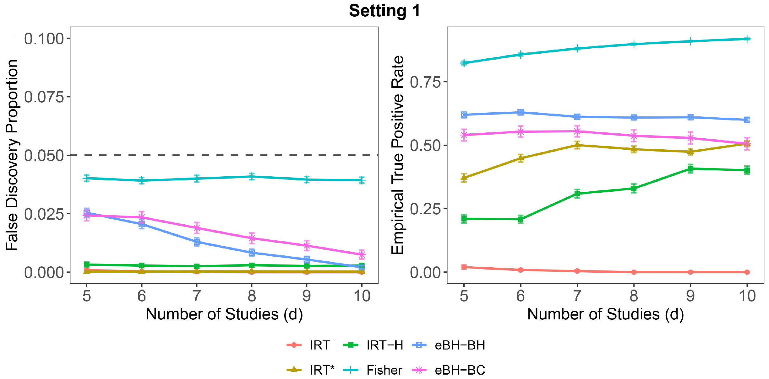
  • Setting 1.
In Setting 1, we consider J independent studies. We would like to test the hypotheses H 0 i : μ i = 0 versus H 1 i : μ i 0 , where the effect sizes are generated from the mixture distribution μ i 0.8 δ ( 0 ) + 0.1 N ( 3 , 1 ) + 0.1 N ( 3 , 1 ) . For study j { 1 , , J } and hypothesis i { 1 , , m j } , we generate
X j , i μ i , σ j ind . N ( μ i , σ j 2 ) , σ j i . i . d . Unif ( 0.75 , 2 ) .
We set m j = m for all j and vary the number of studies J { 5 , 6 , , 10 } . When the null distribution of the test statistic is correctly specified and the resulting p-values are mutually independent, Fisher’s combination test is expected to have higher power than the competing methods. Additionally, in this setting, all methods have theoretical FDR control.
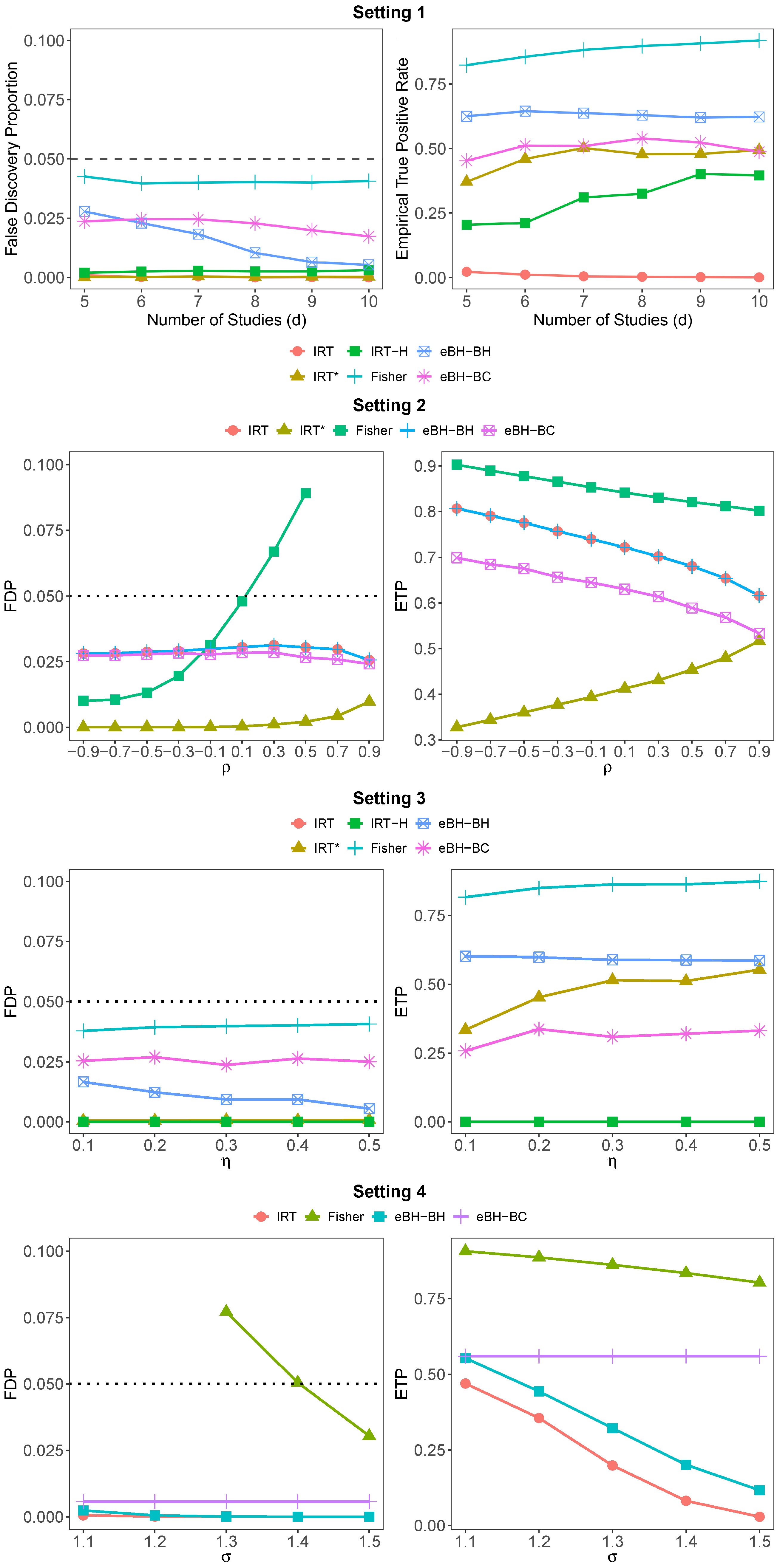
Figure 1 displays the average FDP and ETP across methods. As expected, the Fisher method outperforms the alternatives. Relative to the IRT-based method, the proposed eBH-BC and eBH-BH achieve better performance, with eBH-BH outperforming eBH-BC in this setting. Among the IRT-based procedures, IRT performs best, whereas the standard IRT procedure exhibits nearly zero power.
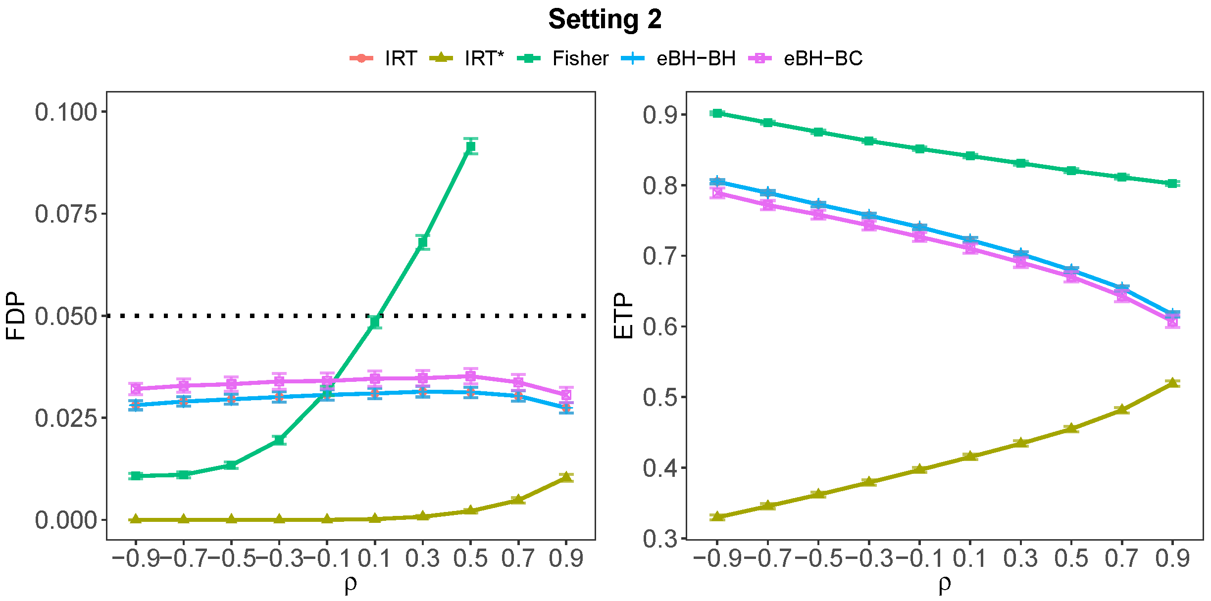
  • Setting 2.
In Setting 2, we allow dependence across J = 2 studies and evaluate methods using one-sided p-values. Specifically, we test H 0 i : μ i = 0 versus H 1 i : μ i > 0 , where μ i i . i . d . 0.8 δ ( 0 ) + 0.2 N ( 3 , 1 ) . Conditional on μ i , the study-level statistics are jointly Gaussian: for each i,
( X 1 , i , , X d , i ) N ( μ i 1 d , Σ ) , Σ j j = σ j 2 = 1 , Σ j k = ρ for j k ,
i.e., Corr ( X j , i , X k , i ) = ρ for all j k . We vary ρ over a grid of equally spaced values in [ 0.9 , 0.9 ] .
Figure 2 reports the average FDP and ETP across methods. In this setting, Fisher, eBH-BC, and IRT do not have theoretical FDR guarantees. Empirically, eBH-BC and IRT control the FDR, whereas Fisher exhibits FDR inflation, especially for large ρ ; accordingly, we omit some points of Fisher from the FDP plot because its average FDP often exceeds the y-axis limit of 0.1. In terms of power, eBH-BH and IRT perform similarly, with eBH-BC slightly less powerful. Notably, in this setting IRT outperforms IRT, in contrast to Setting 1.
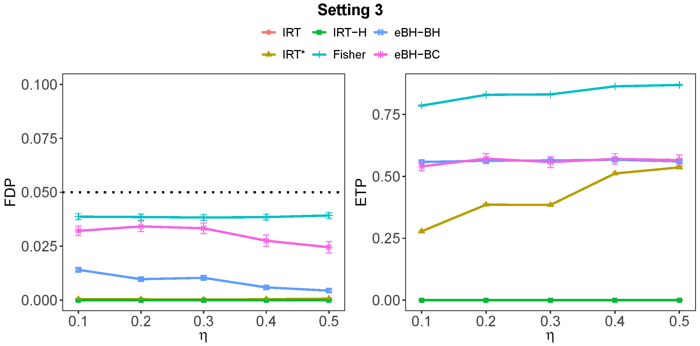
  • Setting 3.
In Setting 3, the data are generated as in Setting 1 with σ j = 1 for all j, and  J = 5 , but we allow the study-specific numbers of tested hypotheses m j to vary across the J studies. We fix the maximum across studies at m max = max { m 1 , , m d } = 900 and define the imbalance ratio ζ = min { m 1 , , m d } / m max ( 0 , 1 ] . For a given ζ , we draw m 1 , , m d independently and uniformly from the integers in [ ζ m max , m max ] . Given these m j ’s, for each study j we then select m j hypotheses uniformly at random without replacement from the m total hypotheses.
Figure 3 reports the average FDP and ETP across methods. In this independent setting, all methods have theoretical FDR control, and Fisher again attains the highest power. Among the IRT-based methods, only IRT achieves nontrivial power, whereas IRT and IRT_H exhibit negligible power. For the proposed methods, eBH-BH and eBH-BC perform similarly and both outperform IRT.
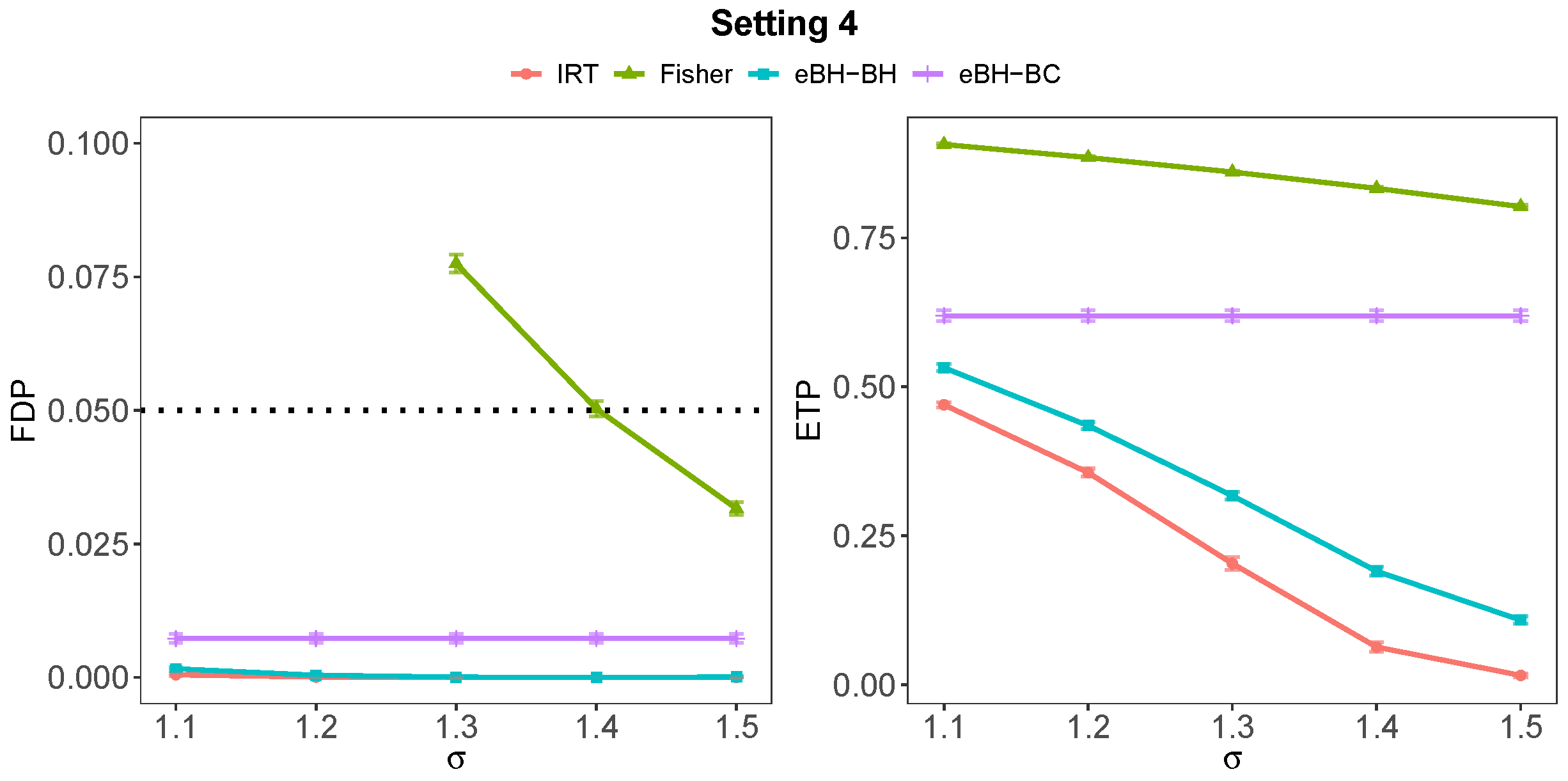
  • Setting 4.
In Setting 4, we consider a scenario in which the study-specific p-values are conservative, under which eBH-BC is more stable and achieves higher power than eBH-BH. Specifically, we set m j = m for all j and J = 5 . For study j and hypothesis i, the summary statistics satisfy X j , i N ( μ i , 1 ) , where the effects μ i are i.i.d. from the mixture 0.8 δ ( 0 ) + 0.2 N ( 3 , 1 ) . We test H 0 i : μ i = 0 versus H 1 i : μ i > 0 , and compute p-values as p i j = Φ ( X j , i / σ ) for σ { 1.1 , 1.2 , 1.3 , 1.4 , 1.5 } . Thus, as  σ increases, the p-values become more conservative. To induce dependence across studies, we set Cov ( X j , i , X k , i ) = 0.5 for all j k (for each fixed i).
Figure 4 reports the average FDP and ETP across methods. In this dependent setting, Fisher and eBH-BC lack theoretical FDR guarantees. While eBH-BC empirically control the FDR, Fisher exhibits inflation. Therefore, Fisher results exceeding the 0.1 y-axis limit are excluded from the FDP plot. From Setting 2, the IRT method performed best among IRT-based procedures; hence, we display only IRT here. In this setting, eBH-BC performs best, and its power does not decrease as the p-values become more conservative. By contrast, the power of the other methods decreases with increasing conservativeness. Additionally, eBH-BH outperforms IRT in all cases.

5. Real Data Analysis

We illustrate the proposed methods using J = 4 publicly available microarray studies of human prostate cancer. These include datasets from Welsh et al. [22] ( m 1 = 8799 ), Singh et al. [23] ( m 2 = 8798 ), Nanni et al. [24] ( m 3 = 12,688), and Wallace et al. [25] ( m 4 = 9703 ). These datasets were also utilized in Banerjee et al. [9]. For each study j { 1 , , J } , the observed data consist of an expression matrix X j with dimension m j × d j , where m j denotes the number of genes profiled and d j denotes the sample size. Each sample is labeled as either case or control. The hypothesis for each gene i within a study is a two-group test for differential expression. After merging features across platforms and mapping probe sets to genes, we obtained a total of m = 16,779 unique genes.
Our objective is to apply the proposed methods to produce a unified list of rejected genes, thereby aggregating evidence across studies to improve the reliability of the results. Before analysis, we merged features across platforms by gene symbol, removed probes with missing or duplicated mappings, and applied standard normalization as implemented in the limma pipeline. In each study, we first employed the limma package [26] to fit gene-wise linear models and compute vectors of p-values. We set the target FDR level for each individual study at 0.05 and the overall target FDR level at 0.1 . We implemented the proposed methods, eBH-BH and eBH-BC, and compared them against IRT and P2E. The P2E algorithm is an e-value-based method implemented in Banerjee et al. [9]; we refer readers to that work for implementation details.
The results of the analysis are presented in Table 1. In this setting, IRT yielded no discoveries. Both proposed eBH-based methods significantly outperformed the P2E method by identifying a larger number of differentially expressed genes. We also observed that eBH-BC generated more rejections than eBH-BH. This is likely because the signal in these datasets is dense (with over 1 / 3 of hypotheses rejected by eBH-BC). In such dense signal settings, the BC procedure is often outperformed than the BH procedure, a phenomenon also observed in Arias-Castro and Chen [20] and Li and Zhang [17].

6. Conclusions

Motivated by Li and Zhang [17], we propose a data-dependent weighting framework for aggregating e-values to synthesize discoveries across partially overlapping studies. By combining within-study e-values, the method produces study-integrated e-values that leverage information across studies. Extensive simulations indicate that data-dependent weighting substantially increases power relative to naive averaging, while maintaining finite-sample control of the FDR across a range of realistic scenarios.
Several avenues merit further investigation. First, beyond the BH and BC procedures, extending the framework to additional multiple-testing paradigms, including structure-adaptive methods, would broaden its applicability. Second, developing aggregation strategies that accommodate settings in which different studies implement heterogeneous within-study procedures is a natural next step. Third, building on the equivalence established in Li and Zhang [7], our current construction assigns a fixed e-value to each rejected hypothesis within a study; designing p-to-e calibrations that preserve more information from the original p-values while maintaining e-value validity remains an important direction for future work.

Author Contributions

Conceptualization, G.L.; methodology, J.G. and G.L.; formal analysis, J.G. and G.L.; investigation, J.G. and H.C.; writing—original draft preparation, G.L.; writing—review and editing, J.G. and H.C.; funding acquisition, G.L. All authors have read and agreed to the published version of the manuscript.

Funding

G.L. was supported by the Fundamental Research Funds for the Central Universities and the National Natural Science Foundation of China, Grant No. 12501350.

Data Availability Statement

The data and code presented in this study are openly accessible from 25 December 2025 and are available in https://drive.google.com/drive/folders/1xSmA-RadQPjCmk1d5s6k6ZqzxC9ZtzB_?usp=sharing and https://github.com/guanxunli/ddwea-fusion/.

Conflicts of Interest

The authors declare no conflicts of interest.

Appendix A. Proofs of Main Results

We first state the following propositions which will be used in the subsequent proofs.
Proposition A1 
(Lemma 6 of Barber et al. [18]). Let T i be the threshold for the BC method when p i is replaced with min { p i , 1 p i } . For any i, j, if  min ( p i , p j ) 1 max { T i , T j } , then we have T i = T j .
Proof. 
Given a p-value vector p = ( p 1 , , p n ) , define
g ( p , t ) : = 1 + l = 1 n 1 { 1 p l t } l = 1 n 1 { p l t } , 0 < t < 0.5 ,
and recall that the threshold for the BC procedure is
T = max 0 < t < 0.5 :   g ( p , t ) α .
For each i { 1 , , n } , set p ˜ i : = min { p i , 1 p i } and
p i : = ( p 1 , , p i 1 , p ˜ i , p i + 1 , , p n ) ,
and define
T i : = max 0 < t < 0.5 :   g ( p i , t ) α .
Fix i j . Without loss of generality, assume T i T j . Suppose moreover that
max { 1 p i , 1 p j } max { T i , T j } = T i .
Then 1 p i T i < 0.5 and 1 p j T i < 0.5 , which imply
p i > 0.5 and p j > 0.5 .
In particular, p i > T i and p j > T i .
Consider
g ( p j , T i ) = 1 + l = 1 n 1 { 1 p j , l T i } l = 1 n 1 { p j , l T i } , where p j , l is the l - th entry of p j .
We compare the denominator and numerator with those of g ( p i , T i ) .
For the denominator,
l = 1 n 1 { p j , l T i } = l = 1 n 1 { p i , l T i } + 1 { p j , j T i } = 1 + 1 { p j , i T i } = 0 1 { p i , j T i } = 0 1 { p i , i T i } = 1 .
Indeed, p j , j = p ˜ j = 1 p j T i (so the first underbrace equals 1), p j , i = p i > T i (so the second underbrace equals 0), p i , j = p j > T i (third underbrace equals 0), and  p i , i = p ˜ i = 1 p i T i (fourth underbrace equals 1). Hence,
l = 1 n 1 { p j , l T i } = l = 1 n 1 { p i , l T i } .
Similarly, for the numerator,
l = 1 n 1 { 1 p j , l T i } = l = 1 n 1 { 1 p i , l T i } + 1 { 1 p j , j T i } = 0 + 1 { 1 p j , i T i } = 1 1 { 1 p i , j T i } = 1 1 { 1 p i , i T i } = 0 .
Here, 1 p j , j = 1 ( 1 p j ) = p j > T i (first underbrace equals 0), 1 p j , i = 1 p i T i (second underbrace equals 1), 1 p i , j = 1 p j T i (third underbrace equals 1), and  1 p i , i = 1 ( 1 p i ) = p i > T i (fourth underbrace equals 0). Therefore,
l = 1 n 1 { 1 p j , l T i } = l = 1 n 1 { 1 p i , l T i } .
Combining the two displays yields
g ( p j , T i ) = g ( p i , T i ) .
By definition of T i , we have g ( p i , T i ) α ; hence g ( p j , T i ) α , which implies T i T j by maximality of T j . Thus T i = T j . □
Proof of Theorem 1.
Let R j ( p j , i 0 ) denote the number of rejections in study j when the p-value p j , i is replaced by 0. By a leave-one-out argument, for any j N i , i = 1 , , m , we have
E [ w j , i e j , i ] = E T j , i T j , i + l j , l N i T l , i · 1 T j 1 { p j , i T j } = i H 0 k = 1 m E T j , i T j , i + l j , l N i T l , i · 1 T j ( k ) 1 { p j , i T j ( k ) , R j ( p j , i 0 ) = k } ,
where the second equality uses the fact that if the ith hypothesis is rejected (i.e., p j , i T j ), then T j = T j , i .
Let F i denote the σ -algebra generated by { p l , i } l N i . Conditioning on F i , we obtain
k = 1 m E T j , i T j , i + l j , l N i T l , i · 1 T j ( k ) 1 { p j , i T j ( k ) , R j ( p j , i 0 ) = k } | F i = k = 1 m T j , i T j , i + l j , l N i T l , i · 1 T j ( k ) P ( p j , i T j ( k ) ) E [ 1 { R j ( p j , i 0 ) = k } F i ] T j , i l N i T l , i ,
since all T l , i for l N i are measurable with respect to F i . Thus,
E [ e i ] = j N i E [ w j , i e j , i ] 1 ,
for any i = 1 , , m , by construction. Therefore,
i H 0 E [ e i ] i H 0 1 m .
 □
Proof of Theorem 2.
Let F j , i denote the σ -algebra generated by { p 1 , , p j 1 , p j , i , p j + 1 , , p m } . By a leave-one-out argument, for any j N i , i = 1 , , m , we have
E [ w j , i e j , i ] = E 1 + l M j , l i 1 { p j , l 1 T j } 1 + l M j , l i 1 { p j , l 1 T j } + s j l M s 1 { p s , l 1 T s , l } × m 1 { p j , i T j } 1 + l M j 1 { p j , l 1 T j } = E E m 1 { p j , i T j , i } 1 + l M j , l i 1 { p j , l 1 T j , i } + s j l M s 1 { p s , l 1 T s , l } | F j , i = E m 1 + l M j , l i 1 { p j , l 1 T j , i } + s j l M s 1 { p s , l 1 T s , l } × E [ 1 { p j , i T j , i } F j , i ] ] E m 1 + l M j , l i 1 { p j , l 1 T j , i } + s j l M s 1 { p s , l 1 T s , l } × E [ 1 { p j , i 1 T j , i } F j , i ] ] = E m 1 { p j , i 1 T j , i } 1 + l M j , l i 1 { p j , l 1 T j , i } + s j l M s 1 { p s , l 1 T s , l } ,
where:
(i)
the second equality uses the fact that T j , i = T j whenever p j , i T j ;
(ii)
in the third equality, both T j , i and T s , l (for s j , l M s ) are F j , i -measurable;
(iii)
the inequality follows from assumption (6).
By Proposition A1, we have
1 { p j , i 1 T j , i } 1 + l M j , l i 1 { p j , l 1 T j , i } + s j l M s 1 { p s , l 1 T s , l } = 1 { p j , i 1 T j , i } l M j 1 { p j , l 1 T j , l } + s j l M s 1 { p s , l 1 T s , l } .
Indeed, if p j , i < 1 T j , i , both sides are zero, so the equality holds trivially. If  p j , i 1 T j , i , we claim that
1 p j , l 1 T j , i = 1 p j , i 1 T j , l .
If p j , l < 1 T j , i but p j , l 1 T j , l , then T j , i < T j , l , which further implies
min { p j , i , p j , l } = p j , l 1 T j , l = 1 max { T j , i , T j , l } .
By Proposition A1, we have T j , i = T j , l , which contradicts the assumption T j , i < T j , l . The converse follows analogously.
Hence,
1 { p j , i 1 T j , i } 1 + l M j , l i 1 { p j , l 1 T j , i } + s j l M s 1 { p s , l 1 T s , l } = 1 { p j , i 1 T j , i } l M j 1 { p j , l 1 T j , l } + s j l M s 1 { p s , l 1 T s , l } = 1 { p j , i 1 T j , i } s = 1 J l M s 1 { p s , l 1 T s , l } .
Therefore,
i = 1 m E [ e i ] = j = 1 J i M j E [ w j , i e j , i ] = j = 1 J i M j E m 1 { p j , i 1 T j , i } s = 1 J l M s 1 { p s , l 1 T s , l } m .
Proof of Theorem 3.
Define the leave-one-out vector
p ˜ l , i = [ p l , 1 , , p l , i 1 , p l , i + 1 , , p l , m ] ,
and let F ˜ j , i be the σ -algebra generated by { p ˜ l , i } l N i , l j { p j , i } . By a leave-one-out argument and the tower property, for any i { 1 , , m } and any j N i ,
E [ w j , i e j , i ] = E 1 + l M j , l i 1 { p j , l 1 T j } 1 + l M j , l i 1 { p j , l 1 T j } + sup q [ 0 , 1 ] s j l M s 1 { p s , l 1 T s , l , i q } × m 1 { p j , i T j } 1 + l M j 1 { p j , l 1 T j } = E E m 1 { p j , i T j , i } 1 + l M j , l i 1 { p j , l 1 T j , i } + sup q [ 0 , 1 ] s j l M s 1 { p s , l 1 T s , l , i q } | F ˜ j , i = E m 1 + l M j , l i 1 { p j , l 1 T j , i } + sup q [ 0 , 1 ] s j l M s 1 { p s , l 1 T s , l , i q } × E [ 1 { p j , i T j , i } F ˜ j , i ] ] E m 1 + l M j , l i 1 { p j , l 1 T j , i } + sup q [ 0 , 1 ] s j l M s 1 { p s , l 1 T s , l , i q } × E [ 1 { p j , i 1 T j , i } F ˜ j , i ] ] = E m 1 { p j , i 1 T j , i } 1 + l M j , l i 1 { p j , l 1 T j , i } + sup q [ 0 , 1 ] s j l M s 1 { p s , l 1 T s , l , i q } E m 1 { p j , i 1 T j , i } 1 + l M j , l i 1 { p j , l 1 T j , i } + s j l M s 1 { p s , l 1 T s , l } ,
where:
(i)
the second equality uses that T j , i = T j whenever p j , i T j ;
(ii)
in the third equality, both T j , i and T s , l , i q (for s j , l M s , q [ 0 , 1 ] ) are F ˜ j , i -measurable, so the inner expectation is taken only over p j , i ;
(iii)
the first inequality follows from Assumption (6);
(iv)
the second inequality follows since
s j l M s 1 { p s , l 1 T s , l } sup q [ 0 , 1 ] s j l M s 1 { p s , l 1 T s , l , i q } ,
i.e., by taking q = p j , i , for which T s , l , i q = T s , l .
Following the same argument as in the proof of Theorem 2, we obtain
i = 1 m E [ e i ] m .

Appendix B. Additionally Numerical Results

Appendix B.1. Additional Numerical Results for Varying Numbers of Hypotheses

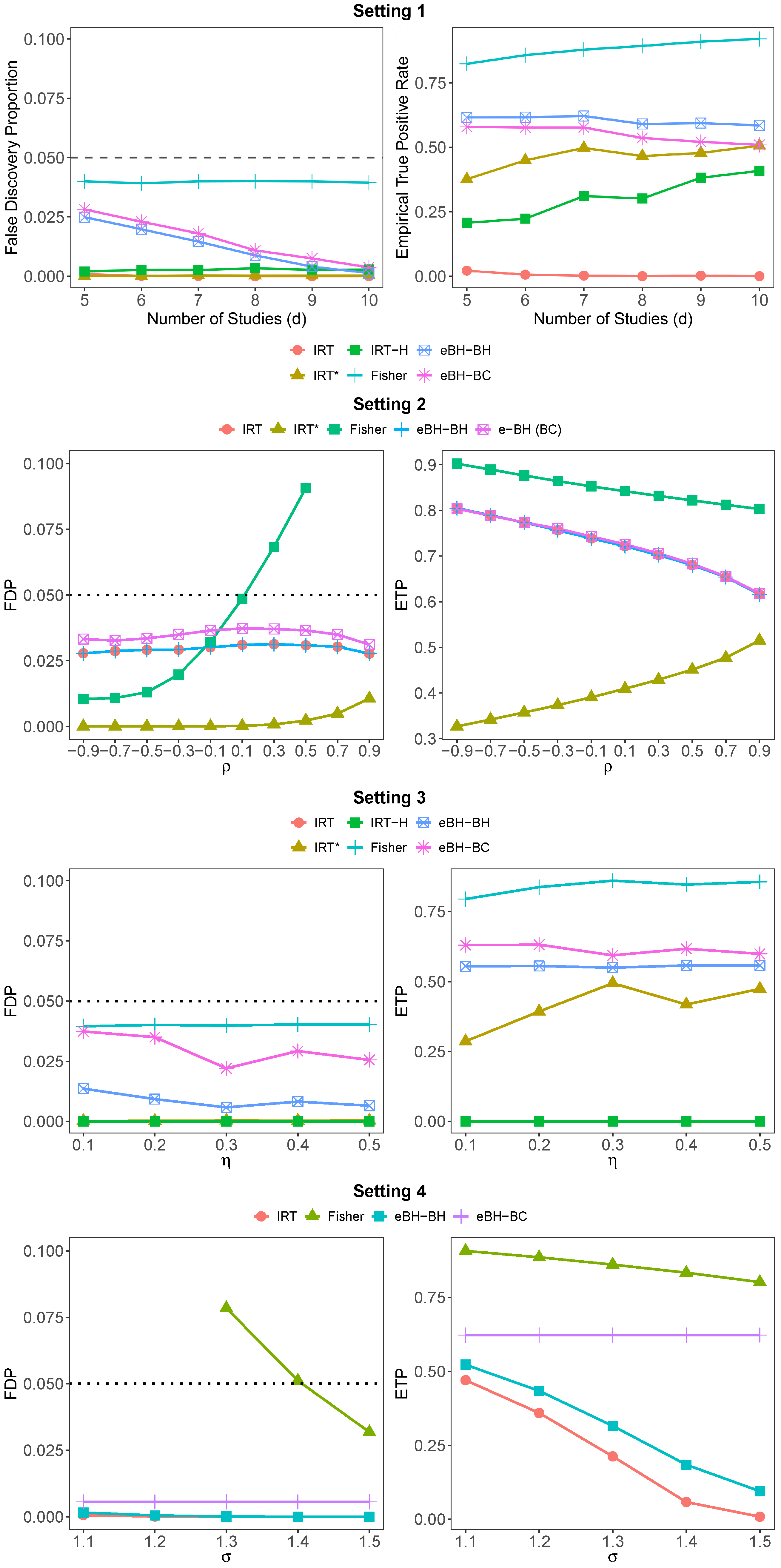
In the main text, we fixed the number of hypotheses at m = 1000 , following Banerjee et al. [9]. Here we report results for other values of m. Figure A1 and Figure A2 show the results for m = 500 and m = 1500 , respectively, across all four settings. The qualitative findings mirror those in the main text and can be summarized as follows:
1.
Fisher’s combination test outperforms the alternatives when hypotheses are independent across studies, but it fails to control the FDR under dependence.
2.
All other methods empirically control the FDR.
3.
eBH-BC and eBH-BH generally outperform the IRT-based method in most cases.
4.
eBH-BC performs best when the study-specific p-values are conservative.
  • Moreover, as m increases, the relative performance of eBH-BC improves compared with the other methods.

Appendix B.2. Additionally Numerical Results for Varying Target FDR Level

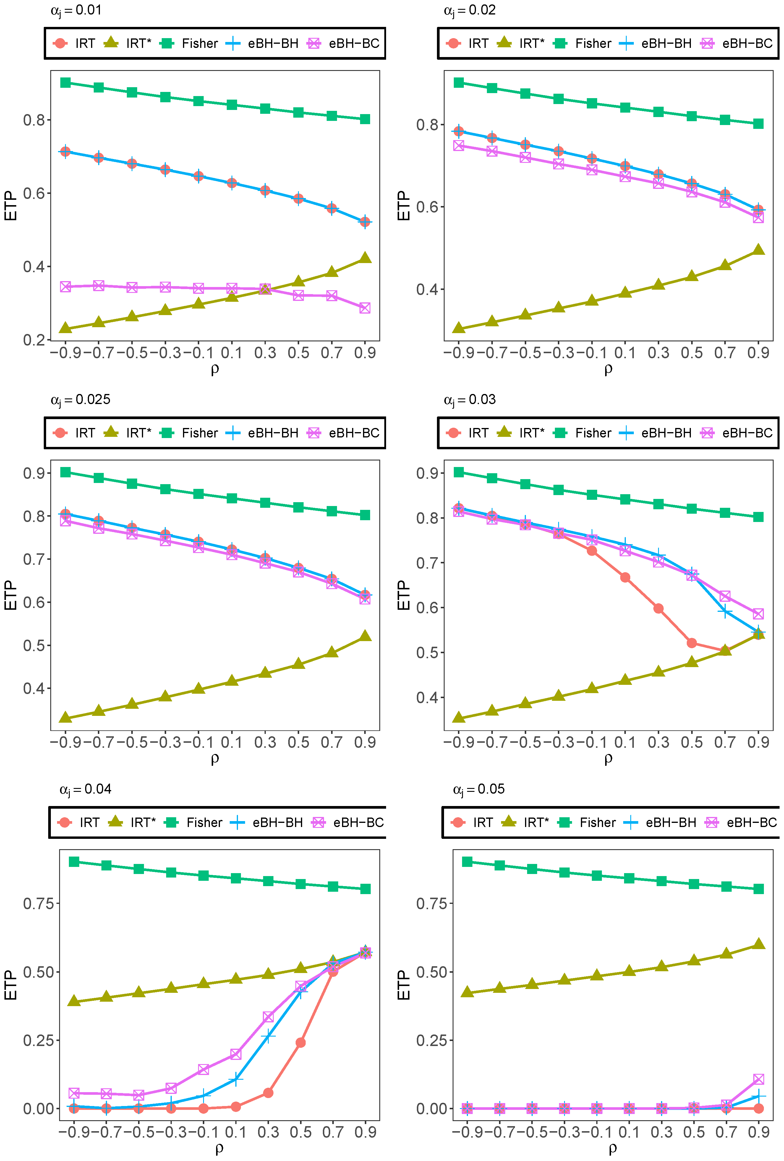
This section discusses the choice of the per-study level α j and the target FDR level α . Following Section 3.2 of Ren and Barber [16], the proposed method achieves adequate power only when α j < α , and they further recommend taking α j < α / 2 . To assess the sensitivity of power to α j of our proposed method, we fix Setting 3 (the dependent setting), set α = 0.05 , and vary α j { 0.01 , 0.02 , 0.025 , 0.03 , 0.04 , 0.05 } . The resulting power and FDR are shown in Figure A3.
The figures indicate that all methods control the FDR. Regarding power, when α j α / 2 , the power of the proposed method increases as α j increases, reflecting the conservativeness of very small α j . However, once α j exceeds approximately 0.04 , the power drops sharply, a phenomenon also reported by Ren and Barber [16].
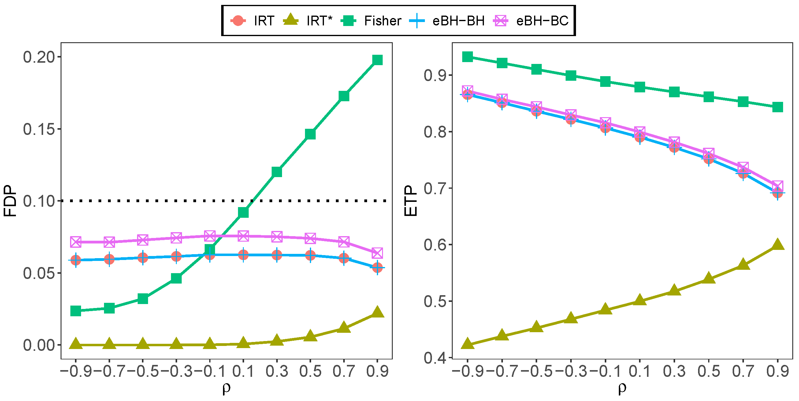
We also examined the pair α j = 0.05 and α = 0.1 ; see Figure A4. The qualitative behavior is the same as described above, and eBH-BH and eBH-BC perform particularly well.
Figure A1. Average FDP and ETP across methods among different settings with m = 500 .
Mathematics 14 00088 g0a1
Figure A2. Average FDP and ETP across methods among different settings with m = 1500 .
Mathematics 14 00088 g0a2
Figure A3. Average ETP across methods in dependent studies (Setting 3) for fixed α and varying α j .
Mathematics 14 00088 g0a3
Figure A4. Average FDP and ETP across methods in independent partially overlapping studies (Setting 3) with α = 0.1 and α j = 0.05 .
Mathematics 14 00088 g0a4

References

  1. Benjamini, Y.; Hochberg, Y. Controlling the false discovery rate: A practical and powerful approach to multiple testing. J. R. Stat. Soc. Ser. B (Methodol.) 1995, 57, 289–300. [Google Scholar] [CrossRef]
  2. Barber, R.F.; Candès, E.J. Controlling the false discovery rate via knockoffs. Ann. Stat. 2015, 43, 2055–2085. [Google Scholar] [CrossRef]
  3. Ignatiadis, N.; Wang, R.; Ramdas, A. Compound e-values and empirical bayes. arXiv 2024, arXiv:2409.19812. [Google Scholar] [CrossRef]
  4. Xu, Z.; Ramdas, A. Online multiple testing with e-values. In Proceedings of the International Conference on Artificial Intelligence and Statistics, PMLR, Valencia, Spain, 2–4 May 2024; pp. 3997–4005. [Google Scholar]
  5. Fischer, L.; Xu, Z.; Ramdas, A. Online generalizations of the e-BH and BH procedure. arXiv 2024, arXiv:2407.20683. [Google Scholar] [CrossRef]
  6. Wang, R.; Ramdas, A. False discovery rate control with e-values. J. R. Stat. Soc. Ser. B Stat. Methodol. 2022, 84, 822–852. [Google Scholar] [CrossRef]
  7. Li, G.; Zhang, X. A note on e-values and multiple testing. Biometrika 2025, 112, asae050. [Google Scholar] [CrossRef]
  8. Liu, D.; Liu, R.Y.; Xie, M.g. Nonparametric fusion learning for multiparameters: Synthesize inferences from diverse sources using data depth and confidence distribution. J. Am. Stat. Assoc. 2022, 117, 2086–2104. [Google Scholar] [CrossRef]
  9. Banerjee, T.; Gang, B.; He, J. Harnessing The Collective Wisdom: Fusion Learning Using Decision Sequences from Diverse Sources. Biometrika 2025, asaf080. [Google Scholar] [CrossRef]
  10. Guo, Z.; Li, X.; Han, L.; Cai, T. Robust inference for federated meta-learning. J. Am. Stat. Assoc. 2025, 120, 1695–1710. [Google Scholar] [CrossRef] [PubMed]
  11. Heimbach, D.; Luterman, A.; Burke, J.; Cram, A.; Herndon, D.; Hunt, J.; Jordan, M.; McManus, W.; Solem, L.; Warden, G. Artificial dermis for major burns. A multi-center randomized clinical trial. Ann. Surg. 1988, 208, 313. [Google Scholar] [CrossRef]
  12. Andres-Terre, M.; McGuire, H.M.; Pouliot, Y.; Bongen, E.; Sweeney, T.E.; Tato, C.M.; Khatri, P. Integrated, multi-cohort analysis identifies conserved transcriptional signatures across multiple respiratory viruses. Immunity 2015, 43, 1199–1211. [Google Scholar] [CrossRef]
  13. Shafi, A.; Nguyen, T.; Peyvandipour, A.; Nguyen, H.; Draghici, S. A multi-cohort and multi-omics meta-analysis framework to identify network-based gene signatures. Front. Genet. 2019, 10, 159. [Google Scholar] [CrossRef]
  14. Kohavi, R.; Tang, D.; Xu, Y.; Hemkens, L.G.; Ioannidis, J.P. Online randomized controlled experiments at scale: Lessons and extensions to medicine. Trials 2020, 21, 150. [Google Scholar] [CrossRef] [PubMed]
  15. Vovk, V.; Wang, R. E-values: Calibration, combination and applications. Ann. Stat. 2021, 49, 1736–1754. [Google Scholar] [CrossRef]
  16. Ren, Z.; Barber, R.F. Derandomised knockoffs: Leveraging e-values for false discovery rate control. J. R. Stat. Soc. Ser. B Stat. Methodol. 2024, 86, 122–154. [Google Scholar] [CrossRef]
  17. Li, G.; Zhang, X. A General Framework for Multiple Testing via E-value Aggregation and Data-Dependent Weighting. arXiv 2025, arXiv:2312.02905. [Google Scholar]
  18. Barber, R.F.; Candès, E.J.; Samworth, R.J. Robust inference with knockoffs. Ann. Stat. 2020, 48, 1409–1431. [Google Scholar] [CrossRef]
  19. Zhao, H.; Zhou, H. τ-censored weighted Benjamini–Hochberg procedures under independence. Biometrika 2024, 111, 479–496. [Google Scholar] [CrossRef]
  20. Arias-Castro, E.; Chen, S. Distribution-free multiple testing. Electron. J. Stat. 2017, 11, 1983–2001. [Google Scholar] [CrossRef]
  21. Fisher, R.A. Combining independent tests of significance. Am. Stat. 1948, 2, 30. [Google Scholar]
  22. Welsh, J.B.; Sapinoso, L.M.; Su, A.I.; Kern, S.G.; Wang-Rodriguez, J.; Moskaluk, C.A.; Frierson, H.F., Jr.; Hampton, G.M. Analysis of gene expression identifies candidate markers and pharmacological targets in prostate cancer. Cancer Res. 2001, 61, 5974–5978. [Google Scholar] [PubMed]
  23. Singh, D.; Febbo, P.G.; Ross, K.; Jackson, D.G.; Manola, J.; Ladd, C.; Tamayo, P.; Renshaw, A.A.; D’Amico, A.V.; Richie, J.P.; et al. Gene expression correlates of clinical prostate cancer behavior. Cancer Cell 2002, 1, 203–209. [Google Scholar] [CrossRef]
  24. Nanni, S.; Narducci, M.; Della Pietra, L.; Moretti, F.; Grasselli, A.; De Carli, P.; Sacchi, A.; Pontecorvi, A.; Farsetti, A. Signaling through estrogen receptors modulates telomerase activity in human prostate cancer. J. Clin. Investig. 2002, 110, 219–227. [Google Scholar] [CrossRef][Green Version]
  25. Wallace, T.A.; Prueitt, R.L.; Yi, M.; Howe, T.M.; Gillespie, J.W.; Yfantis, H.G.; Stephens, R.M.; Caporaso, N.E.; Loffredo, C.A.; Ambs, S. Tumor immunobiological differences in prostate cancer between African-American and European-American men. Cancer Res. 2008, 68, 927–936. [Google Scholar] [CrossRef] [PubMed]
  26. Ritchie, M.E.; Phipson, B.; Wu, D.; Hu, Y.; Law, C.W.; Shi, W.; Smyth, G.K. Limma powers differential expression analyses for RNA-sequencing and microarray studies. Nucleic Acids Res. 2015, 43, e47. [Google Scholar] [CrossRef] [PubMed]
Figure 1. Average FDP and ETP across methods in the independent-studies setting (Setting 1). Error bars indicate ±2 standard errors. The x-axis shows the number of independent studies. Fisher denotes Fisher’s combination test; IRT, IRT-H, and IRT are three integrative ranking-and-thresholding (IRT) methods; eBH-BH and eBH-BC are the proposed e-value aggregation methods with data-dependent weights.
Mathematics 14 00088 g001
Figure 2. Average FDP and ETP across methods in dependent setting (Setting 2). Error bars indicate ±2 standard errors. The x-axis shows the correlation between dependent studies. Fisher denotes Fisher’s combination test; IRT and IRT are two Integrative Ranking and Thresholding (IRT)-based methods; eBH-BH and eBH-BC are the two proposed e-value aggregation methods with data-dependent weights.
Mathematics 14 00088 g002
Figure 3. Average FDP and ETP across methods in independent partially overlapping studies (Setting 3). Error bars indicate ± 2 standard errors. The x-axis ζ quantifies cross-study imbalance as the ratio of the smallest to the largest study-specific number of tested hypotheses. Fisher denotes Fisher’s combination test; IRT, IRT H and IRT* are three Integrative Ranking and Thresholding (IRT)-based methods; eBH-BH and eBH-BC are the two proposed e-value aggregation methods with data-dependent weights.
Mathematics 14 00088 g003
Figure 4. Average FDP and ETP across methods in conservative and dependent setting (Setting 4). Error bars indicate ±2 standard errors. The x-axis σ parameterizes the degree of conservativeness in the study-specific p-values. Fisher denotes Fisher’s combination test; IRT and IRT are two Integrative Ranking and Thresholding (IRT)-based methods; eBH-BH and eBH-BC are the two proposed e-value aggregation methods with data-dependent weights.
Mathematics 14 00088 g004
Table 1. Number of rejections for different methods across the real data sets.
MethodIRTP2EeBH-BHeBH-BC
Number of Rejections0149431236314
Disclaimer/Publisher’s Note: The statements, opinions and data contained in all publications are solely those of the individual author(s) and contributor(s) and not of MDPI and/or the editor(s). MDPI and/or the editor(s) disclaim responsibility for any injury to people or property resulting from any ideas, methods, instructions or products referred to in the content.