Analytical Solutions and Analyses for the Deflection of Nonlinear Waves on Kirchhoff Plates Underlying a Pasternak-like Nonlinear Elastic Foundation

Abstract

The present study models the deflection of nonlinear waves over a Kirchhoff plate underlying a Pasternak-like elastic foundation. A promising version of the tanh expansion analytical method has been deployed for the construction of regular exact solutions for the model, including the application of certain ansatz functions for validations and yet construction of more solutions. The resulting frequency equation and the modulation instability spectrum have been obtained for the linearized model, including the expressions for the related phase and group velocities. In addition, the study examines the equilibrium status of the resulting dynamical system with the help of the bifurcation analysis. Numerically, nonlinear deflection and dispersion of waves have been simulated through the acquired expressions and equations. Notably, the study notes that increasing both the Pasternak-like nonlinear parameter $\eta$ and time variation (for $x>0$) decreases the nonlinear deflection in the plate, while increasing the stiffness of the Winkler foundation increases deflection in the medium. In addition, the study establishes, concerning the determined frequency equation, that increasing the Winkler foundation stiffness increases the dispersion of nonlinear waves in the medium, while an opposite trend has been noted concerning the imposed Pasternak-like nonlinear foundation. In addition, both phase and group velocities, the gain function for modulation instability, and the resulting dynamical system have been noted to be greatly affected by the variation of the imposed foundational parameters. Lastly, this study has potential applications in various engineering fields while modeling and analysis of mechanical structures supported by additional structures.

1. Introduction

The deflection and propagation of edge waves in elastic plates have been characterized with vast relevance in contemporary fields of engineering applications, including fields like the structural engineering, civil engineering, aerospace and marine engineering, and in the construction of biomedical and miniature structures, among others, where engineers and modelers make use of the fundamentals of elasticity to perfectly model the governing momentum equation(s) of motion(s) [1,2,3]. The quest for structural stability and optimization concerning material, size, and durability is all directed towards the optimal setting for the geometrical and structural configuration [4,5]. Mathematically, various theorists have proposed different models for the deflection of linear waves in plates and beams, even though modern, realistic processes have shown that nonlinearities emerge in most practical applications. Thus, this study is directed towards the study of nonlinear deflection in beams and plates. Besides this, linear deflections in plates have been extensively studied in both recent and past scripts concerning both the methodology and application. As an instance, Althobaiti et al. [6] gave an account for how a moving surface loading affects the deflection of waves in orthotropic plates using the Fourier integral transform method; Althobaiti and Prikazchikov [7] examined the dispersion of bending edge waves over an elastic plate, while Althobaiti and Hawwa [8] modeled the deflection of flexural waves over an induced piezoelectric plate through harmonic wave analysis. Moreover, recent studies have featured the significance of incorporating external forces and internal effects, including thermal stress force, foundational supports, and porosities, among others, into the dynamics of plates and beams—see the recent findings reported in Kumari et al. [9], Althobaiti et al. [6] and Althobaiti and Prikazchikov [7], to state but a few. Furthermore, as foundational supports further enrich the structural stability of the plates, in addition to other industrial and engineering applications of elastic foundations, Wang et al. [10] have perfectly captured the use of various forms of elastic foundations, and some of the well-known methods in the study of linear deflection plates placed on elastic foundations. In addition, the work by Doyle and Pavlovic [11] on modeling the impact of weak foundational supports on the vibration of flexural waves has been greatly acknowledged, while that of Zhou [12] on the effect of moving Winkler foundation on the dispersion of flexural waves has received numerous applauds. Accordingly, the optimal choice of materials in multilayered plates has been a matter of much concern industrially. Thus, Schulze et al. [13] described the propagation of bending of waves and material characterization in composite plates, and Sayyad and Ghugal [14] described the bending of waves in multiple-layered beams. In addition, Sahin [15] adopted the asymptotic analysis technique to describe the low-frequency deflection in an elastic plate, and the work by Sahin et al. [16], which proposed an approximation method for bending characterization in elastic beam-plates. What is more, the reader is referred to the recent works by Ebrahimi and Seyfi [17], Erbas et al. [18], and Mubaraki [19], among others, which examined various wave scenarios concerning the presence of foundational supports attached to the governing elastic structures. However, in all the aforementioned references, interaction of elastic plates and structures with dissimilar foundational supports was examined while the involved elastic foundations were linear. In the light of this, a burning curiosity emerged, which resulted in an in-depth search into literature and able to the identification of a few works that examined nonlinear foundational supports in structures. In this regard, it is very pertinent to mention the study by Fu [20] that theoretically examined, through an asymptotic approach, the stability aspect of an elastic beam underlying a nonlinear foundation. Moreover, even though the work by Fu [20] is aimed at examining the stability of elastic structures subjected to superior deformations asymptotically, however, one ones the presence of nonlinear deflection in favour of the imposed nonlinear foundation amidst the attendance of bifurcated terms. In addition, the study by Lenci and Clementi [21] described a sort of foundational support using a unilateral function that takes into account a nonlinearity possibility. What is more, the paper by Collet and Pouget [22] explicitly proposed a nonlinear elastic foundational support into the dynamics of flexural waves deflection on a thin plate under the action of initial pre-stresses. Therefore, with the study by Collet and Pouget [22], various studies follow suit with dissimilar nonlinear foundational supports, including the recent study by Althobaiti et al. [23], which analytically examines the deflection of plates underlying three different forms of nonlinear foundations. In fact, the presence of nonlinear terms in the model changes the overall setting of the equations. Thus, looking at these equations as nonlinear evolution equations, researchers for exact solutions of differential equations have proposed various analytical methods for analytical analysis. In this regard, some of the promising methods used to construct exact solitonic equations include the modified extended tanh function method [24], the Kudryashov technique [25], the improved version of Kudryashov technique [26], ansatz method using exponential function [27], the Hirota bilinear method [28], the symmetry technique by Lie [29], the Adomian method of decomposition [30], the variational iteration approach [31], the auxiliary equation method [32], the improved version of the auxiliary equation method [33], and the enhanced modified Sardar-sub equation method [34], among others.

However, with the advent of the studies by, specifically Collet and Pouget [22], and the recent study by Althobaiti et al. [23] on the propagation of bending flexural waves geared by a nonlinear foundation, this study thus models the deflection of nonlinear waves over a Kirchhoff plate that rests on a Pasternak-like nonlinear elastic foundation.Moreover, classical Pasternak elastic foundation [5,10] was improved upon the original Winkler foundation to account for two parameters for the stiffness of the material for the foundational supports, and that of the accompanying Pasternak spring. Beside, several applications of elastic foundations have been greatly noted in physical systems that require the stiffness of the foundation to exhibit nonlinearity properties; uses of such foundations have been identified in the control of vibrations in plates and beams [35], among others. Equally, such kind of foundations have been observed in to perfectly model real-world engineering applications, including underground structures, and rail ways, and are further noted to be highly relevant in the structural design and analysis of modern structures in mechanical, civil and structural engineering to mention a few [36,37]. Thus, in this study, a Pasternak-like nonlinear elastic foundation is introduced, with the accomplishment of the findings in [22,23]. In addition, the said modified extended tanh method [24] will be deployed for the analytical investigation of the model, including seeking the help of certain ansatz function methods [27,38] for validation and more solutions. In addition, the resulting frequency equation of the linearized model will be acquired and analyzed, including the acquisition of the subsequent expressions for the phase and group velocities. Further, the modulation instability spectrum will be examined in the study, coupled with the analysis of the bifurcation possibility of the resulting dynamical system. More so, numerical results will be presented through numerical simulation and will characterize the overall deflection dynamics in the medium. Lastly, this study is organized in the form that follows: Section 2 gives the outline of the basic equations. Section 3 states the statement of the aiming problem. Section 4 gives the outline of the adopted analytical technique and the acquired solutions by the adopted method. Section 5 presents the resulting frequency equation and the modulation study. Section 6 gives the dynamical study of the model. Section 7 presents the numerical results and discussion, while Section 8 provides some recaps of the work achieved.

2. Governing Equation for Kirchhoff Plates

We consider the equation of motion, over an isotropic plate that occupys the area $-\infty <x_1<\infty ,$ $0\le x_2<\infty ,$ $-h\le x_3\le h,$ to be governed by the shear forces, and bending moments equations, respectively, in tensorial form as follows [39]

$$\begin{array}{cc}\hfill N_{x_1{x}_1,x_1}+N_{x_1{x}_2,x_2}& =\rho {u_1}_{\tau \tau },\hfill \\ \hfill N_{x_1{x}_2,x_1}+N_{x_2{x}_2,x_2}& =\rho {u_2}_{\tau \tau },\hfill \end{array}$$

(1)

and

$$\begin{array}{cc}\hfill M_{x_1{x}_1,x_1{x}_1}+2M_{x_1{x}_2,x_1{x}_2}+M_{x_2{x}_2,x_2{x}_2}& =\rho h{u_3}_{\tau \tau },\hfill \end{array}$$

(2)

where $N_{ij}$, and $M_{ij}$ for $i=j=x_1,x_2,x_3$ are in-plane forces, and bending moments, respectively, defined as

$$\begin{array}{cc}\hfill N_{ij}& ={\int }_{-h/2}^{h/2}{\sigma }_{ij}d{x}_3,M_{ij}={\int }_{-h/2}^{h/2}{x}_3{\sigma }_{ij}d{x}_3,\hfill \end{array}$$

(3)

where, $u_k=u_k(x_1,x_2,\tau )$ for $k=1,2,3$ are displacement (deflection) fields in the spatial variables $x_1,x_2$ and the temporal variable $\tau .$ In addition h is the half-thickness of the plate, $\rho$ is the density of the material; while the variable that follows after the respective commas signifies a derivative with the respective to that variable. More so, ${u_1}_{\tau \tau }={\displaystyle \frac{{\partial }^2{u}_1}{\partial {\tau }^2}},$ and ${u_2}_{\tau \tau }={\displaystyle \frac{{\partial }^2{u}_2}{\partial {\tau }^2}},$ and ${u_3}_{\tau \tau }={\displaystyle \frac{{\partial }^2{u}_3}{\partial {\tau }^2}},$ are the accelerations. What is more, ${\sigma }_{ij}$ is the related stress tensor [8,39], while the displacement fields $u_1$ and $u_2$ are further re-considered as follows

$$\begin{array}{cc}\hfill u_1& =-x_3{u}_{3,x_1},u_2=-x_3{u}_{3,x_2},\hfill \end{array}$$

(4)

where $u_3$ is the longitudinal displacement field. Thus, without much delay, and further considering the field $u_3=\overline{u},$ one obtains the governing equation for the deflection of flexural waves, from the above equations, on an isotropic plate as follows

$$D\overline{\Delta }\overline{\Delta }\overline{u}+2\rho h{\overline{u}}_{\tau \tau }=0,$$

(5)

where $\overline{u}=\overline{u}(x_1,x_2,\tau ),$ is the displacement fields in the spatial variables $x_1,x_2$ and time variable $\tau ,$ while $\rho ,h$ and D are the density, half-thickness, and the stiffness of the plate, respectively. Additionally, $\overline{\Delta }$ is the Laplacian operator, defined as

$$\overline{\Delta }={\displaystyle \frac{{\partial }^2}{\partial x_1^2}}+{\displaystyle \frac{{\partial }^2}{\partial x_2^2}},\overline{\Delta }\overline{\Delta }={\displaystyle \frac{{\partial }^4}{\partial x_1^4}}+2{\displaystyle \frac{{\partial }^4}{\partial x_1^2\partial x_2^2}}+{\displaystyle \frac{{\partial }^4}{\partial x_2^4}}.$$

(6)

In particular, with the consideration of the two-parameter elastic foundation [5], the so-called Pasternak foundation, which is assumed to occupy the area $-\infty <x_1<\infty ,$ $0<x_2<\infty ,$ $2h\le x_3\le \infty ,$ renders Equation (5) to be re-expressed as follows

$$D\overline{\Delta }\overline{\Delta }\overline{u}+\beta \overline{u}-c\overline{\Delta }\overline{u}+2\rho h{\overline{u}}_{\tau \tau }=0,$$

(7)

where $\beta$ and c are the stiffnesses of the Winkler elastic foundation, and the Pasternak spring, respectively. What is more, when $c=0$ in the latter equation, the so-called Pasternak foundation reduces to the Winkler elastic foundation, which was asymptotically examined in [5]. Moreover, when both c and $\beta$ vanished, Equation (7) returns to Equation (5).

Notably, Equation (7) can equally be re-expressed in form as follows [5]

$$\overline{\Delta }\overline{\Delta }\overline{u}+{\lambda }^{-4}\overline{u}-2{\chi }^{-2}\overline{\Delta }\overline{u}+{\lambda }^{-4}\ddot{\overline{u}}=0,$$

(8)

where the characteristic lengths $\lambda$ and $\chi$ take the following expressions

$$\lambda ={\displaystyle \frac{\sqrt[4]{D}}{\sqrt[4]{\beta }}},\mathrm{and}\chi ={\displaystyle \frac{\sqrt{2D}}{\sqrt{c}}},$$

(9)

where the double dots in $\overline{u}$ stands for the second differentiation with respect to the dimensionless time variable $t=\tau \sqrt{\beta }/\sqrt{2\rho h}.$ Moreover, with the consideration of the following a positive dimensionless ratio $\eta$ as

$${\eta }_1={\displaystyle \frac{\lambda }{\chi }}=\sqrt[4]{{\displaystyle \frac{c^2}{4\beta D}}},$$

(10)

coupled with the dimensionless coordinates x and y as follows

$$x={\displaystyle \frac{x_1}{\lambda }},\mathrm{and}y={\displaystyle \frac{x_2}{\lambda }},$$

(11)

thereby re-expressing Equation (8) as follows

$$\Delta \Delta u+u-2{\eta }_1^2\Delta u+\ddot{u}=0,$$

(12)

where $u=u(x,y,t)$ in the displacement field in the spatial variables $x,y$ and the temporal variable $t.$

3. Problem Statement

Motivated by the insufficient works in the literature about the significance of nonlinear elastic foundations on the deflection of elastic plates, this study thus aims to consider a nonlinear Pasternak-like elastic foundation attached to the governing Kirchhoff plate, as discussed in Equation (7), and subsequently modified in Equation (12) as follows

$$\Delta \Delta u+\xi u-\eta \Delta u^2+\ddot{u}=0,$$

(13)

where $u=u(x,y,t)$ is the displacement field in space $x,y$ and t time variables, and $\xi ,$ and $\eta$ are systematically scaled parameters to account for the effects of the stiffness of the Winkler foundation and Pasternak-like nonlinear spring, respectively. Moreover, in the absence of the nonlinearity, and setting $\xi =1,$ and $\eta =2{\eta }_1^2,$ one recovers Equation (12) from Equation (13). In this regard, it is pertinent to mention here that the related stiffness of the nonlinear Pasternak-like foundation $\eta$ is dimensionless, with the consideration of $\eta =2{\eta }_1^2/h,$ while stiffness of the Winkler foundation $\xi$ is presumed to lie within $0<\xi \le 1,$ affirming the adopted dimensionalization of the earlier Equation (12). Besides, one captures the situation of realizing soft Winkler elastic foundation $\xi <<1$ [18]. Additionally, $\Delta$ in Equation (13) is the Laplacian operator, defined as

$$\Delta ={\displaystyle \frac{{\partial }^2}{\partial x^2}}+{\displaystyle \frac{{\partial }^2}{\partial y^2}},\Delta \Delta ={\displaystyle \frac{{\partial }^4}{\partial x^4}}+2{\displaystyle \frac{{\partial }^4}{\partial x^2\partial y^2}}+{\displaystyle \frac{{\partial }^4}{\partial y^4}}.$$

(14)

Accordingly, one re-expresses Equation (13) through Equation (14) more explicitly to obtain the following nonlinear equation of motion as follows

$$u_{xxxx}+2u_{xxyy}+u_{yyyy}+\xi u-\eta \left({\left(u^2\right)}_{xx}+{\left(u^2\right)}_{yy}\right)+u_{tt}=0,$$

(15)

where $\xi$ and $\eta$ account for the effects of the stiffness of the Winkler foundation and Pasternak-like nonlinear spring, respectively.

What is more, a couple of analytical methods will be utilized in the present study to investigate Equation (15) concerning the existence, or rather the admittance of assorted analytical solutions. In addition, the equation will equally be examined to get a general view of how elastic waves disperse in the plate; of course, this will be carried out after the equation is first linearized. In addition, the modulation instability of the system will also be studied. Lastly, the equation will be equally analyzed through its resulting dynamical system for the bifurcation analysis version. Thus, several graphical depictions will be supplied in the end. Besides, it will be pertinent to mention here that a few researchers investigated the action of simple nonlinear foundations on the dispersion of nonlinear edge waves, including quadratic forms by [22,23], and the quadratic, cubic, and quadratic-cubic nonlinearities by Saad et al. [23], among others. In particular, Saad et al. [23] analyzed the quadratic-cubic nonlinear foundation with initial pre-stresses in the plate equation as follows

$$u_{xxxx}+2u_{xxyy}+u_{yyyy}+\mu u_{xx}+\lambda u_{yy}+\xi u-{\eta }_1{u}^2-{\eta }_2{u}^3+u_{tt}=0,$$

(16)

where $\mu$ and $\lambda$ are the respective longitudinal and transverse initial pre-stresses, while $\xi$ is the stiffness of the Winkler foundation, and ${\eta }_1$ and ${\eta }_2$ are constants due to the quadratic and cubic nonlinear foundations, correspondingly. Beside, one may equally consult some of the very recent advances on well-posedness, regularity and asymptotic behavior of the dynamic Kirchhoff equation in the works of Li et al. [40], and Arora et al. [41], among others that examined the relevance of weak solutions to Kirchhoff problems in high dimensions amidst a logarithmic type perturbation, and the state-of-the-art of a Kirchhoff-type model that includes a nonlinear term of sub-critical growth and a parametric singular term, respectively. These studies are indeed very apt for formalization, in addition to being a monograph for foundational perspective on Kirchhoff plate model in modern times; see also the studies by Lv [42], and Shibata [43] that provided contemporary mathematical literature on the physical regime, which the adopted nonlinear foundation model remains meaningful.

4. Construction of Displacement Fields

4.1. Adopted Analytical Method

To begin with, the governing model in Equation (15) is first transformed to its corresponding ordinary differential equation using the following wave transformation

$$u(x,y,t)=V\left(\vartheta \right),\vartheta =k(x+y)-\omega t$$

(17)

as follows

$$G\left(V\left(\vartheta \right),V^{\prime }\left(\vartheta \right),V^{″}\left(\vartheta \right),V^{″\prime }\left(\vartheta \right),\dots \right)=0,$$

(18)

where the primes ${\{}^{\prime }{,}^{″}{,}^{″\prime },\dots \}$ in $V\left(\vartheta \right)$ above are derivatisations.

In this regard, the adopted analytical is the renown modified tanh expansion method, which further assumed the latter differential equation in Equation (18) to be satisfied by the follows presumed series solution [24]

$$V\left(\vartheta \right)=\sum _{j=0}^N{f}_j{\varphi }^j\left(\vartheta \right)+\sum _{j=1}^N{g}_j{\varphi }^{-j}\left(\vartheta \right),$$

(19)

where $f_0,f_j,$ and $g_j,$ for $j=1,2,3,\dots$ are constants, which not all equal zero that are be determined, while N is a positive integer, which is equally to be determined by balancing the highest linear (differential) and nonlinear terms in the governing equation using the following relations

$$\begin{array}{c}\hfill D\left\{V^X\left(\vartheta \right)\right\}=XN,D\left\{{\displaystyle \frac{d^{Y}V\left(\vartheta \right)}{d{\vartheta }^Y}}\right\}=N+Y,D\left\{V^X\left(\vartheta \right){\left({\displaystyle \frac{d^{Z}V\left(\vartheta \right)}{d{\vartheta }^Z}}\right)}^W\right\}=XN+W(N+Y),\end{array}$$

(20)

where $W,X,Y$ and Z are whole numbers, D stands for the degree of the bracketed term(s).

In particular, the infused function $\varphi \left(\vartheta \right)$ in Equation (19) has been noted to satisfy the following first-order nonlinear differential equation

$${\varphi }^{\prime }\left(\vartheta \right)=s+{\varphi }^2\left(\vartheta \right),$$

(21)

where $s\ne 0$ is a real number. What is more, Equation (21) satisfies the following exact solutions

(i).

For $s=0$,

$$\begin{array}{c}\hfill \varphi \left(\vartheta \right)=-{\displaystyle \frac{1}{\vartheta }}.\end{array}$$

(22)

(ii).

For $s<0$, one gets the following hyperbolic solutions

$$\begin{array}{c}\hfill \varphi \left(\vartheta \right)=\left\{-\sqrt{-s}coth\left(\sqrt{-s}\vartheta \right),\sqrt{-s}tanh\left(\sqrt{-s}\vartheta \right)\right\}.\end{array}$$

(23)

(iii).

For $s>0$, one gets the following periodic solutions

$$\begin{array}{c}\hfill \varphi \left(\vartheta \right)=\left\{-\sqrt{s}cot\left(\sqrt{s}\vartheta \right),\sqrt{s}tan\left(\sqrt{s}\vartheta \right)\right\}.\end{array}$$

(24)

Therefore, upon substituting the presumed solution in Equation (19) together with its respective derivatives into the reduced differential equation in Equation (18), of course, through Equations (22) and (23), one gets an algebraic system of equations that will be solved for the explicit expressions for $f_0, f_j, g_j(j\ge 1)$ and s. Consequently, dissimilar exact solutions for Equation (18) are obtained, which further yields the solution of the governing partial differential equation through Equation (17). Remarkably, this study makes use of the Wolfram Mathematica 9.0 for the computational purpose.

4.2. Displacement Fields by the Adopted Method

Accordingly, with the presented method in the above subsection, one deploys the wave transformation in Equation (17) into the governing nonlinear beam equation in Equation (15) to thus obtain the following nonlinear differential equation

$$V^{\left(4\right)}\left(\vartheta \right)+{\displaystyle \frac{{\omega }^2}{4k^4}}{V}^{″}\left(\vartheta \right)+{\displaystyle \frac{\xi }{4k^4}}V\left(\vartheta \right)-{\displaystyle \frac{\eta }{k^2}}V\left(\vartheta \right)V^{″}\left(\vartheta \right)-{\displaystyle \frac{\eta }{k^2}}{V}^{\prime }{\left(\vartheta \right)}^2=0.$$

(25)

Next, the homogeneous balance, between the highest linear derivative term and the nonlinear term in the latter equation, that is, between

$$V^{\left(4\right)}\left(\vartheta \right)\mathrm{and}V\left(\vartheta \right)V^{″}\left(\vartheta \right),\mathrm{or}{V}^{\left(4\right)}\left(\vartheta \right)\mathrm{and}{V}^{\prime }\left(\vartheta \right),$$

(26)

both yield the natural number N as follows

$$N=2.$$

(27)

Consequently, Equation (26) admits, through Equation (19), the following solution form

$$V\left(\vartheta \right)=f_0+f_1\varphi \left(\vartheta \right)+f_2{\varphi }^2\left(\vartheta \right)+g_1{\varphi }^{-1}\left(\vartheta \right)+g_2{\varphi }^{-2}\left(\vartheta \right),$$

(28)

where $f_0,f_j(j=12)$ and $g_j(j=1,2),$ are constants (not all zero) that will be determined. Moreover, substituting Equation (28), alongside Equation (21), into the nonlinear differential equation in Equation (26) gives a system of algebraic equations as follows

$$480g_2{k}^4{s}^4-40\eta g_2^2{k}^2{s}^2=0,96g_1{k}^4{s}^4-48\eta g_1{g}_2{k}^2{s}^2=0,$$

$$-24f_0\eta g_2{k}^2{s}^2+960g_2{k}^4{s}^3-12\eta g_1^2{k}^2{s}^2-64\eta g_2^2{k}^{2}s+6g_2{s}^2{\omega }^2=0,$$

$$-8f_0\eta g_1{k}^2{s}^2-8f_1\eta g_2{k}^2{s}^2+160g_1{k}^4{s}^3-72\eta g_1{g}_2{k}^{2}s+2g_1{s}^2{\omega }^2=0,$$

$$-32f_0\eta g_2{k}^{2}s+544g_2{k}^4{s}^2-24\eta g_2^2{k}^2-16\eta g_1^2{k}^{2}s+g_2\xi +8g_{2}s{\omega }^2=0,$$

$$-8f_0\eta g_1{k}^{2}s-8f_1\eta g_2{k}^{2}s+64g_1{k}^4{s}^2-24\eta g_1{g}_2{k}^2+g_1\xi +2g_{1}s{\omega }^2=0,$$

$$-8f_2\eta g_1{k}^{2}s+64f_1{k}^4{s}^2-24f_1{f}_2\eta k^2{s}^2-8f_0{f}_1\eta k^{2}s+f_1\xi +2f_{1}s{\omega }^2=0,$$

$$544f_2{k}^4{s}^2-24f_2^2\eta k^2{s}^2-16f_1^2\eta k^{2}s-32f_0{f}_2\eta k^{2}s+f_2\xi +8f_{2}s{\omega }^2=0,$$

$$-8f_2\eta g_1{k}^2+160f_1{k}^{4}s-8f_0{f}_1\eta k^2-72f_1{f}_2\eta k^{2}s+2f_1{\omega }^2=0,480f_2{k}^4-40f_2^2\eta k^2=0,$$

$$960f_2{k}^{4}s-12f_1^2\eta k^2-24f_0{f}_2\eta k^2-64f_2^2\eta k^{2}s+6f_2{\omega }^2=0,96f_1{k}^4-48f_1{f}_2\eta k^2=0,$$

$$-8f_0\eta g_2{k}^2+64f_2{k}^4{s}^3-4f_1^2\eta k^2{s}^2-8f_0{f}_2\eta k^2{s}^2+f_0\xi +2f_2{s}^2{\omega }^2+64g_2{k}^{4}s-4\eta g_1^2{k}^2+2g_2{\omega }^2=0.$$

Accordingly, in what follows, the later the algebraic system is solved, where several solution sets are revealed.

4.2.1. Rational Displacement Fields When $s=0$

Here, upon solving the resulting algebraic system of of nonlinear (which was omitted for brevity) for $s=0$ from Equation (21), one obtains two solution sets for propagation of rational solution fields, including

$$Set\left(1\right):f_0=-{\displaystyle \frac{{\omega }^2}{8\eta k^2}},f_1=0,f_2=0,g_1=0,g_2={\displaystyle \frac{\xi }{24\eta k^2}},$$

(29)

which yields the following rational displacement field

$$u(x,y,t)={\displaystyle \frac{-{\omega }^2}{8\eta k^2}}+{\displaystyle \frac{\xi {(k(x+y)-\omega t)}^2}{24\eta k^2}},$$

(30)

and

$$Set\left(2\right):f_0={\displaystyle \frac{48{\eta }^2{g}_1^2{k}^4-\xi {\omega }^2}{8\eta k^2\xi }},f_1=0,f_2=0,g_1=g_1,g_2={\displaystyle \frac{\xi }{24\eta k^2}},$$

(31)

that reveals the following rational displacement field

$$u(x,y,t)={\displaystyle \frac{48{\eta }^2{g}_1^2{k}^4-\xi {\omega }^2}{8\eta k^2\xi }}-g_1(k(x+y)-\omega t)+{\displaystyle \frac{\xi {(k(x+y)-\omega t)}^2}{24\eta k^2}}.$$

(32)

4.2.2. Hyperbolic Displacement Fields When $s<0$

Equally, with the consideration of $s<0$ from Equation (21), two hyperbolic solution sets are obtained, which give rise to the construction of hyperbolic displacement fields for the governing nonlinear model as follows

$$Set\left(1\right):f_0={\displaystyle \frac{32k^{4}s+{\omega }^2}{4\eta k^2}},f_1=0,f_2=\left\{0,{\displaystyle \frac{12k^2}{\eta }}\right\},g_1=0,g_2=\left\{{\displaystyle \frac{12k^2{s}^2}{\eta }},0\right\},\xi =0,$$

(33)

that leads to the acquisition of the following singular solitonic solution

$$\begin{array}{cc}\hfill u(x,y,t)& ={\displaystyle \frac{32k^{4}s+{\omega }^2}{4\eta k^2}}-{\displaystyle \frac{12k^{2}s{coth}^2\left(\sqrt{s}(k(x+y)-\omega t)\right)}{\eta }},\hfill \end{array}$$

(34)

and the following dark solitonic solution

$$\begin{array}{cc}\hfill u(x,y,t)& ={\displaystyle \frac{32k^{4}s+{\omega }^2}{4\eta k^2}}-{\displaystyle \frac{12k^{2}s{tanh}^2\left(\sqrt{s}(k(x+y)-\omega t)\right)}{\eta }}.\hfill \end{array}$$

(35)

In addition, the solution of the system equally yields the following hyperbolic solution set

$$Set\left(2\right):f_0={\displaystyle \frac{32k^{4}s+{\omega }^2}{4\eta k^2}},f_1=0,f_2={\displaystyle \frac{12k^2}{\eta }},g_1=0,g_2={\displaystyle \frac{12k^2{s}^2}{\eta }},\xi =0,$$

(36)

that leads to the realization of the following dark-singular solitonic solution

$$u(x,y,t)={\displaystyle \frac{32k^{4}s+{\omega }^2}{4\eta k^2}}-{\displaystyle \frac{12k^{2}s{tanh}^2\left(\sqrt{s}(k(x+y)-\omega t)\right)}{\eta }}-{\displaystyle \frac{12k^{2}s{coth}^2\left(\sqrt{s}(k(x+y)-\omega t)\right)}{\eta }}.$$

(37)

4.2.3. Periodic Displacement Fields When $s>0$

In the same manner, considering $s>0$ from Equation (21), two periodic solution sets are obtained through the adopted modified extended tanh method for the governing nonlinear model as follows

$$Set\left(1\right):f_0={\displaystyle \frac{32k^{4}s+{\omega }^2}{4\eta k^2}},f_1=0,f_2=\left\{0,{\displaystyle \frac{12k^2}{\eta }}\right\},g_1=0,g_2=\left\{{\displaystyle \frac{12k^2{s}^2}{\eta }},0\right\},\xi =0,$$

(38)

which reveals the following periodic solutions

$$\begin{array}{cc}\hfill u(x,y,t)& ={\displaystyle \frac{32k^{4}s+{\omega }^2}{4\eta k^2}}+{\displaystyle \frac{12k^{2}s{cot}^2\left(\sqrt{s}(k(x+y)-\omega t)\right)}{\eta }},\hfill \end{array}$$

(39)

and

$$\begin{array}{cc}\hfill u(x,y,t)& ={\displaystyle \frac{32k^{4}s+{\omega }^2}{4\eta k^2}}+{\displaystyle \frac{12k^{2}s{tan}^2\left(\sqrt{s}(k(x+y)-\omega t)\right)}{\eta }}.\hfill \end{array}$$

(40)

Accordingly, the algebraic system, when solved yields the second solution set for the examining model as follows

$$Set\left(2\right):f_0={\displaystyle \frac{32k^{4}s+{\omega }^2}{4\eta k^2}},f_1=0,f_2={\displaystyle \frac{12k^2}{\eta }},g_1=0,g_2={\displaystyle \frac{12k^2{s}^2}{\eta }},\xi =0,$$

(41)

which precisely leads to the following periodic solution for the nonlinear beam equation

$$u(x,y,t)={\displaystyle \frac{32k^{4}s+{\omega }^2}{4\eta k^2}}+{\displaystyle \frac{12k^{2}s{tan}^2\left(\sqrt{s}(k(x+y)-\omega t)\right)}{\eta }}+{\displaystyle \frac{12k^{2}s{cot}^2\left(\sqrt{s}(k(x+y)-\omega t)\right)}{\eta }}.$$

(42)

4.3. Displacement Fields by Ansatz Method

First, having balanced the governing equation, and identified the positive integer, that is, $N=2$ (see Equations (26) and (27)), we then proceed to deploy ansatz method to equally predicts the existence of certain exact solutions for the nonlinear model. Thus, motivated by the value of N (even though not always helpful in ansatz method), the following ansatz functions are adopted [27]

$$Hyperbolicansatz:V\left(\vartheta \right)=\{A{\csc \mathrm{h}}^2\left(B\vartheta \right),A{\sec \mathrm{h}}^2\left(B\vartheta \right)\},$$

(43)

and

$$Periodicansatz:V\left(\vartheta \right)=\{A{\csc }^2\left(B\vartheta \right),A{\sec }^2\left(B\vartheta \right)\},$$

(44)

where $A,$ and B are non-zero constants to be determined by solving the resulting algebraic equations, as explained in Section 4. Accordingly, upon substituting the ansatz expressed in Equations (43) and (44) into the reduced equation in Equation (25), one gets, after solving the resulting consequential algebraic equations (this algebraic system of equations is ignored for brevity in this case) the following respective solution sets

$$Set\left(1\right):A=\left\{-{\displaystyle \frac{3{\omega }^2}{4\eta k^2}},{\displaystyle \frac{3{\omega }^2}{4\eta k^2}}\right\},B=\left\{\pm i{\displaystyle \frac{\omega }{4k^2}},\pm i{\displaystyle \frac{\omega }{4k^2}}\right\},\xi =0,$$

(45)

and

$$Set\left(2\right):A={\displaystyle \frac{3{\omega }^2}{4\eta k^2}},B=\left\{-{\displaystyle \frac{\omega }{4k^2}},{\displaystyle \frac{\omega }{4k^2}}\right\},\xi =0,$$

(46)

where the above sets collectively yield periodic solutions for the governing nonlinear wave equation as follows

$$u(x,y,t)={\displaystyle \frac{3{\omega }^2}{4\eta k^2}}{csc}^2\left({\displaystyle \frac{\omega }{4k^2}}(k(x+y)-\omega t)\right),$$

(47)

and

$$u(x,y,t)={\displaystyle \frac{3{\omega }^2}{4\eta k^2}}{sec}^2\left({\displaystyle \frac{\omega }{4k^2}}(k(x+y)-\omega t)\right).$$

(48)

Notably, as the imaginary number $i(i^2=-1)$ appears in the solution set in Equation (46), it thus necessitates the resulting solutions to be periodic as reported in the solutions given in Equations (48) and (49).

In the same vein, for more investigation, the following exponential function ansatz is equally adopted [38]

$$Exponentialansatz:V\left(\vartheta \right)=A+B{\displaystyle \frac{exp\left(\vartheta \right)}{{(exp\left(\vartheta \right)+1)}^2}},$$

(49)

where $A,$ and B are equally non-zero constants to be determined. Consequently, on substituting the ansatz in Equation (49) into Equation (25), one gets, after solving the resulting algebraic equations the following respective solution sets

$$Set\left(1\right):A=A,B=-{\displaystyle \frac{12k^2}{\eta }},\omega =\pm 2\sqrt{A\eta k^2-k^4},\xi =0,$$

(50)

which reveals the following hyperbolic solutions

$$u(x,y,t)=A-{\displaystyle \frac{6k^2}{\eta cosh\left(k(x+y)+2t\sqrt{A\eta k^2-k^4}\right)+\eta }},$$

(51)

and

$$u(x,y,t)=A-{\displaystyle \frac{3k^2}{\eta }}{\sec \mathrm{h}}^2\left({\displaystyle \frac{1}{2}}k(x+y)-t\sqrt{A\eta k^2-k^4}\right).$$

(52)

$$Set\left(2\right):A=0,B=-{\displaystyle \frac{12k^2}{\eta }},\omega \pm 2i{k}^2,\xi =0,$$

(53)

with the latter set yielding the periodic and exponential solutions, respectively, as follows

$$u(x,y,t)=-{\displaystyle \frac{3k^2}{\eta }}{sec}^2\left({\displaystyle \frac{1}{2}}k(2kt-i(x+y))\right),$$

(54)

and

$$u(x,y,t)=-{\displaystyle \frac{12k^2{e}^{k(2ikt+x+y)}}{\eta {\left(e^{k(x+y)}+e^{2i{k}^{2}t}\right)}^2}}.$$

(55)

Remarkably, it is very pertinent to mention here that all the acquired solutions in this section are special since the Winkler elastic parameter vanished, that is, $\xi =0,$ except for the reported rational solutions in Equations (30) and (32), which are the only general solutions that feature both the Winkler foundation parameter $\xi ,$ and the nonlinear foundation parameter $\eta .$ Thus, in Section 7, the acquired solution in Equation (32), alongside the dark solitonic solution reported in Equation (35) will be numerically be studied through graphical depiction in Figure 1 and Figure 2, to see how the deflection of the governing nonlinear beam responses to the variation of time t, Winkler elastic parameter $\xi ,$ and the nonlinear foundation parameter $\eta .$ Certainly, the disappearance of the stiffness parameter of the Winkler foundation in many solutions, with the exception of the reported solutions Equations (30) and (32), is admittedly associated with the limitation of the adopted analytical method; however, this limitation is let go since the said solutions are general, and this is the reason the method is not discarded. Moreover, other sophisticated modified methods could equally be employed, including the improved modified extended tanh method [24].

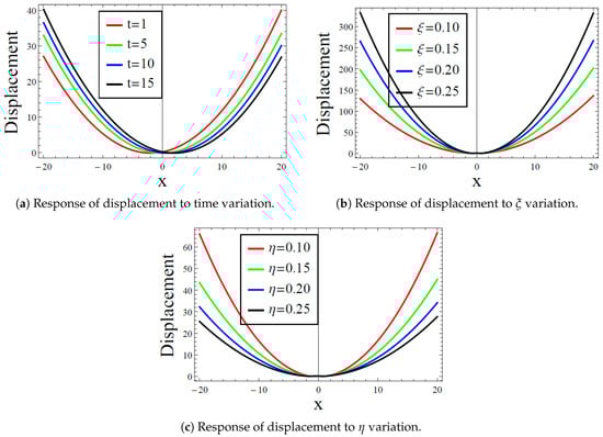
Figure 1. Displacement curve (32) response to the variation in: (a) time variation t when $g_1=-0.3,$ $\xi =0.1,$ $\eta =0.2.$ (b) Winkler foundation parameter $\xi$ when $g_1=-0.26, \eta =0.05, t=1.$ (c) Pasternak-line nonlinear foundation parameter $\eta$ when $g_1=-0.07, t=1, \xi =0.1.$ In addition, other parameters are fixed in all the figures as follows $k=0.6, \omega =0.25,$ $y=x.$

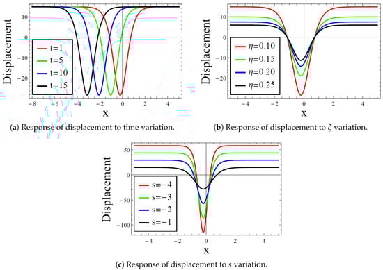
Figure 2. Displacement curve (35) response to the variation in: (a) time variation t when $\xi =0.1,$ $s=-1,$ $\eta =0.1.$ (b) Pasternak-line nonlinear foundation parameter $\eta$ when $t=1, \xi =0.1, s=-1.$ (c) Adopted method foundation parameter s when $\xi =0.1, \eta =0.1, t=1.$ In addition, other parameters are fixed in all the figures as follows $k=0.6, \omega =-0.25,$ $y=x.$

5. Frequency Equation and Modulation Instability

For the analyses of the overall frequency equation and modulation instability concerning the examined nonlinear beam equation, it is mentioned here that the tools at hand only apply to the linear model. Thus, we are left with two options here: (i) disregarding the nonlinear terms, whereby examining the corresponding linear model similar to the study by Kaplunov and Nobili [5], and (ii) linearizing the model, thereby analyzing the resulting linearized model considering a steady-state solution for Equation (15) as follows [44,45]

$$u(x,y,t)=(v(x,y,t)+\sqrt{q})e^{iqt},$$

(56)

where $v(x,y,t)$ is the perturbed displacement field, i is the imaginary unit, with $i^2=-1,$ while q is the incident power; moreover, this study is equally well-informed about other forms of perturbed solutions, aimed at nonlinearization, including the form deployed by Yao et al. [46], which got sense of the modulation instability of the modified Benjamin-Bona-Mohony equation. Accordingly, plugging Equation (56) into Equation (15) yields a linearized (perturbed) model as follows

$$v_{xxxx}+2v_{xxyy}+v_{yyyy}+(\xi -q^2)v+2i{v}_t+v_{tt}=0,$$

(57)

which is a sort of Schrodinger equation with the discovery of imaginary number in the equation. Beside, the utilization of the form in Equation (56) is favour of getting the sense of full temporal variation arising from the involving acceleration in the governing model (see the second to the last term in the latter equation), which the frequency in the later harmonic solution $\omega$ captures.

However, the second option lies in the consideration of the linearized part of Equation (15) as follows

$$u_{xxxx}+2u_{xxyy}+u_{yyyy}+\xi u-\eta (u_{xx}+u_{yy})+u_{tt}=0,$$

(58)

indeed, the equation of plates admits the action of the classical Pasternak foundation. Notably, we utilize the second equation, expressed in Equation (58) in favour of the presence of both $\xi$ and $\eta ,$ the respective stiffnesses Winkler and Pasternak foundation parameters, where $0<\xi \le 1,$ and $\eta =2{\eta }_1^2.$ In this regard, motivated by several studies on the possible modulation instability being posed by solitons and solitary-like wave solutions under the shade of nonlinear evolution equations, this study thus make a consideration of option (ii) to deeply examine the relevance of the involved stiffnesses.

5.1. Frequency Equation

Here, to derive the aiming frequency equation, a harmonic wave solution of the following form is adopted [5,6]

$$u(x,y,t)=A{e}^{i(Kx-\Omega t)-Kpy},$$

(59)

where K is the wave number, $\Omega$ is the frequency, while p is the attenuation parameter. Accordingly, upon substituting the latter assumed solution into Equation (58), one gets the following frequency equation

$$K^4{\left(p^2-1\right)}^2+\eta K^2\left(1-p^2\right)+\xi -{\Omega }^2=0,$$

(60)

where one notes that when the attenuation parameter p is fixed at $p=1,$ the dispersion of the wave in the medium becomes independent of the wave number. Moreover, setting both $\xi$ and $\eta$ to be unity, one gets the dispersion relation reported by Kaplunov and Nobili [5]. In addition, one vividly deduces two special frequency equations from Equation (60) when $\eta =0,$ and $\xi =0,$ respectively, as follows

$$K^4{\left(p^2-1\right)}^2+\xi -{\Omega }^2=0,$$

(61)

and

$$K^4{\left(p^2-1\right)}^2+\eta K^2\left(1-p^2\right)-{\Omega }^2=0,$$

(62)

What is more, one further deduces the related phase and group velocities $V^{ph}$ and $V^g$ from Equation (60), correspondingly, as follows

$$V^{ph}={\displaystyle \frac{\Omega }{K}}={\displaystyle \frac{\sqrt{2}\Omega \sqrt{p^2-1}}{\sqrt{\sqrt{{\eta }^2-4\xi +4{\Omega }^2}+\eta }}},$$

(63)

and

$$V^g={\displaystyle \frac{\mathrm{d}\Omega }{\mathrm{d}K}}={\displaystyle \frac{\sqrt{p^2-1}\sqrt{{\eta }^2-4\xi +4{\Omega }^2}\sqrt{\sqrt{{\eta }^2-4\xi +4{\Omega }^2}+\eta }}{\sqrt{2}\Omega }}.$$

(64)

Notably, upon setting $\eta =\xi =0$ in the above velocities, one gets that both velocities are equal, that is,

$$V^{ph}=V^g=\sqrt{(p^2-1)\Omega }.$$

(65)

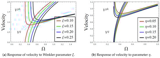
Graphically, both the frequency equation, expressed in Equation (60), and the respective velocities in Equations (63) and (64) will be numerically analyzed through Figure 3 and Figure 4, respectively.

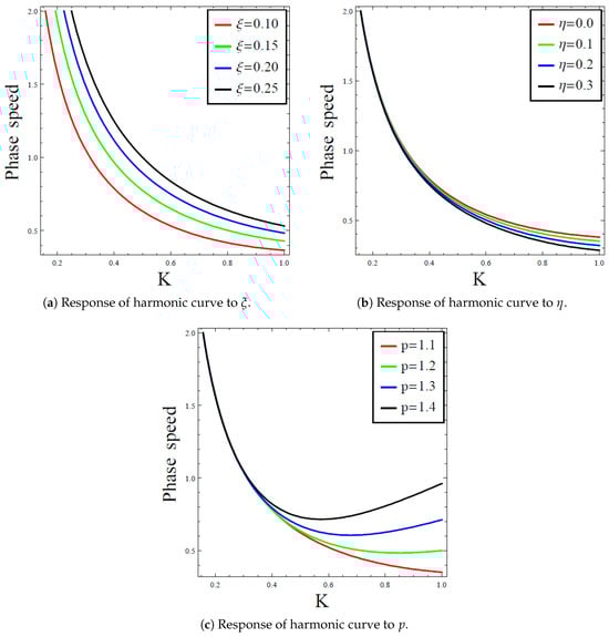
Figure 3. Harmonic curve (60) response to the variation in: (a) Winkler foundation parameter $\xi$ when $p=1.1, \eta =0.05.$ (b) Pasternak-line nonlinear foundation parameter $\eta$ when $p=1.1, \xi =0.1.$ (c) attenuation parameter p when $\eta =0.1, \xi =0.1$.

Figure 4. Response of the phase $V^{ph}$ and group $V^g$ velocities (63) and (64) to variation of: (a) Winkler foundation parameter $\xi$ at $p=1.5, \eta =0.05$. (b) Pasternak-like nonlinear foundation parameter $\eta$ at $p=1.5$, $\xi =0.1$.

5.2. Modulation Instability Analysis

To analyze the expected modulation instability, we again refer to the derived frequency equation in Equation (60) and make the frequency $\Omega$ the subject of the formula as follows

$$\Omega =\pm \sqrt{{\gamma }^2{K}^4-\eta \gamma K^2+\xi },$$

(66)

where

$$\gamma =p^2-1.$$

(67)

Furthermore, an instability in the modulation is expected when the expression under the square root in Equation (66) satisfies the following inequality

$$\gamma K^2+{\displaystyle \frac{\xi }{\gamma K^2}}<\eta .$$

(68)

Remarkably, the expression for $\gamma ,$ as expressed in Equation (68) plays a vital role in this regard, where one can observe a complete modulation stability when $\gamma <0;$ recall that both $\xi$ and $\eta$ for positives, having considered the nonlinear elastic foundation to lay under the governing Kirchhoff plate. In addition, the resulting gain function $G\left(K\right)$ can equally be obtained from Equation (66) as follows

$$G\left(K\right)=2\Im (\Omega ),$$

(69)

where $\Omega$ is expressed in Equation (66), and $\Im (.)$ stands for the imaginary part of the bracketed function; moreover, see Figure 5 for the numerical analysis of the resultant gain function.

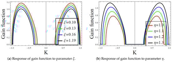
Figure 5. Response of the gain function $G\left(K\right)$ (69) to variation of: (a) Winkler foundation parameter $\xi$ at $p=1.5, \eta =1.33$. (b) Pasternak-like nonlinear foundation parameter $\eta$ at $p=1.5, \xi =0.1.$

6. Bifurcation Analysis

With appropriate Galilean transformation, viz,

$$Y_1=V,Y_2=Y_1^{\prime },Y_3=Y_2^{\prime },Y_4=Y_3^{\prime },$$

(70)

the fourth-order nonlinear differential equation expressed Equation (25), which is the reduced form of the governing nonlinear beam equation is transformed to the system of first-order nonlinear dynamical equations as follows

$$\begin{array}{cc}\hfill Y_1^{\prime }& =Y_2,\hfill \\ \hfill Y_2^{\prime }& =Y_3,\hfill \\ \hfill Y_3^{\prime }& =Y_4,\hfill \\ \hfill Y_4^{\prime }& =({\alpha }_1{Y}_3-{\alpha }_2)Y_1+\left(2{\alpha }_1{Y}_2\right)Y_2+({\alpha }_1{Y}_1-{\alpha }_3)Y_3,\hfill \end{array}$$

(71)

where

$$\begin{array}{c}\hfill {\alpha }_1={\displaystyle \frac{\eta }{2k^2}},{\alpha }_2={\displaystyle \frac{\xi }{4k^4}},\mathrm{and}{\alpha }_3={\displaystyle \frac{{\omega }^2}{4k^4}}.\end{array}$$

(72)

Accordingly, one may obtain the related Hamiltonian from the above dynamical system [47,48], including the subsequent kinetic and potential energy functions. Moreover, to obtain the equilibrium points for the said system, one equates the equations in Equation (71) to zero to get as follows

$$\begin{array}{c}\hfill Y_2=Y_3=Y_4=0,{\alpha }_2{Y}_1=0.\end{array}$$

(73)

Thus, from the last equation in Equation (73), since ${\alpha }_2\ne 0,$ it implies that $Y_1=0.$ Consequently, the only equilibrium point is the trivial one, that is, $E_0=(0,0,0,0).$

Next, we compute the Jacobian determinant of the resulting Jacobian of the system in Equation (71) as follows

$$\begin{array}{c}\hfill det\left(J\right)=\left|\begin{array}{cccc}0& 1& 0& 0\\ 0& 0& 1& 0\\ 0& 0& 0& 1\\ {\alpha }_1{Y}_3-{\alpha }_2& 4{\alpha }_1{Y}_2& {\alpha }_1{Y}_1-{\alpha }_3& 0\end{array}\right|={\alpha }_2-{\alpha }_1{Y}_3.\end{array}$$

(74)

Hence, one realizes the Jacobian determinant determined in Equation (74) at the equilibrium point $E_0$ as follows

$$\begin{array}{c}\hfill {det\left(J\right)|}_{E_0}=-{\alpha }_2.\end{array}$$

(75)

Accordingly, with the realization of the Jacobian determinant at the equilibrium point $E_0$ in Equation (75), one confidently notes the existence of the following scenarios:

(i)

A saddle point when ${det\left(J\right)|}_{E_0}<0;$ which is made possible with the consideration of ${\alpha }_2>0,$

(ii)

A center point when ${det\left(J\right)|}_{E_0}>0;$ which is made possible with the consideration of ${\alpha }_2<0.$

Notably, it is pertinent to recall that ${\alpha }_2={\displaystyle \frac{\xi }{4k^2}},$ where $\xi$ is the stiffness of the Winkler elastic foundation upon which the governing plate is underlyied. In this case, with the accompanying positive sign for $\xi$ in Equation (15), one theoretically placed the elastic foundation above the governing place when $\xi >0;$ while for $\xi <0,$ the plate is assumed to be under the elastic foundation [23]; see [35] for a different interpretation related to the signs of elastic foundations. What is more, for the completeness of the established results, one seeks to further analyze the linearized version of the system in Equation (73); of course, the overall trace of the Jacobian has been noted to be zero. Accordingly, the linearization are obtained from the Jacobian at the equilibrium point $E_0$ as follows

$$\begin{array}{c}\hfill {J|}_{E_0}=\left(\begin{array}{cccc}0& 1& 0& 0\\ 0& 0& 1& 0\\ 0& 0& 0& 1\\ -{\alpha }_2& 0& -{\alpha }_3& 0\end{array}\right),\mathrm{at}{E}_0,\end{array}$$

(76)

which eventually leads to the following linearized system at $E_0$

$$\begin{array}{cc}\hfill Z_1^{\prime }& =Z_2,\hfill \\ \hfill Z_2^{\prime }& =Z_3,\hfill \\ \hfill Z_3^{\prime }& =Z_4,\hfill \\ \hfill Z_4^{\prime }& =-{\alpha }_2{Z}_1-{\alpha }_3{Z}_3.\hfill \end{array}$$

(77)

with the coefficient matrix, being invertible posing the following eigenvalues:

$$\begin{array}{c}\hfill {\lambda }_{1,2}=\pm {\displaystyle \frac{1}{\sqrt{2}}}\sqrt{-{\alpha }_3-\sqrt{{\alpha }_3^2-4{\alpha }_2}},{\lambda }_{3,4}=\pm {\displaystyle \frac{1}{\sqrt{2}}}\sqrt{-{\alpha }_3+\sqrt{{\alpha }_3^2-4{\alpha }_2}}.\end{array}$$

(78)

Noticeably, upon disregarding the Winkler elastic foundation in the model, that is, when $\xi =0,$ which leads ${\alpha }_2=0,$ one gets from the latter eigenvalues

$$\begin{array}{c}\hfill {\lambda }_{1,2}=0,{\lambda }_{3,4}=\pm i\sqrt{{\alpha }_3},\end{array}$$

(79)

which gives a degenerate case. Consequently, several other cases could equally be checked, including for example when ${\alpha }_3^2-4{\alpha }_2>0,$ and $-{\alpha }_3\pm \sqrt{{\alpha }_3^2-4{\alpha }_2}>0,$ which gives real eigenvalues, and posing nodal sink/source, otherwise, the contrary gives complex roots eigenvalues that lead to spirals sink/source or a center as the case maybe. In essence, more analysis is required with the consideration of numerical data.

7. Numerical Results and Discussion

7.1. Displacement Fields Analysis

This subsection gives graphical depictions and discussion for some of the acquired exact analytical solutions for the deflection of nonlinear waves on the governing Kirchhoff plate. In particular, the constructed rational solution in Equation (32), and the dark solitonic solution in Equation (35) will be respectively examined through Figure 1 and Figure 2, correspondingly, as a case of interest. Moreover, the remaining constructed solutions can equally be analyzed in the same manner, which are intentionally left here for conciseness. However, having already stated that the adopted method gives only rational solutions, expressed in Equations (30) and (32), that account for the effect both the stiffness of the Winkler elastic foundation $\xi ,$ and that of the Pasternak-like nonlinear parameter $\eta ,$ Figure 1 thus examines the variational effect, or rather, the response of the nonlinear deflection to time variation in Figure 1a, effect of the Winkler elastic foundation in Figure 1b, and the significance of the varying the Pasternak-like nonlinear parameter in Figure 1c. Notably, one notes from Figure 1a that for $x>0,$ an increase in temporal variation decreases the nonlinear deflection in the plate; see the case, where a reverse trend occurs when $x<0.$ In addition, one notes from Figure 1b that increasing the stiffness of the Winkler foundation increases the deflection in the medium. What is more, an increase in the Pasternak-like nonlinear parameter $\eta$ has been observed to decrease the deflection in the medium, see Figure 1c. In the same vein, Figure 2 basically portrays the same interpretation. Indeed, one notes from Figure 2a that an increase in time variation retrogresses the deflection in the medium, while an increase in the Pasternak-like nonlinear parameter $\eta ,$ and the adopted method parameter $s,$ respectively, decrease the deflection of nonlinear waves in the governing plate as given in Figure 2b,c, correspondingly.

7.2. Frequency Equation and Modulation Instability Analyses

The obtained frequency equation in Equation (60) for the linearized model is analyzed in Figure 3 through phase speed $(\Omega /K)$ versus the wave number (K) plots, while the response of the acquired phase $V^{ph}$ and group $V^g$ velocities in Equations (63) and (64), respectively are examined in Figure 4. In addition, the resulting gain function $G\left(K\right)$, found in Equation (69) for the modulation instability, is examined in Figure 5. Therefore, from Figure 3, one observes how, from Figure 3a, the dispersion of the harmonic waves changes with an increase in the stiffness of the Winkler foundation in an increasing manner. Thus, one can confidently say that an increase in the Winkler foundation stiffness increases the dispersion of waves in the governing isotropic plate. In addition, an opposite trend has been observed in Figure 3b about the increase of the Pasternak-like nonlinear parameter, which vividly decreases the dispersion of waves with an increase in the wave number. Additionally, having originally considered the attenuation parameter p from Equation (59), where one notes from the frequency equation in Equation (60) that there is no attenuation of waves when $p=1,$ including the absence of both the effects of $\xi$ and $\eta .$ Thus, from Figure 3c that an increase in the attenuation parameter increases the dispersion of harmonic waves in the media. Aside, the consideration of the purely Pasternak structural foundation reduces the governing model to the study by Kaplunov and Nobili [5], all the reported findings in [5] can thus be deduced admits the presence of linearization of the model. In the same vein, upon disregarding the structural nonlinear elastic foundation in the present study, one gets the submission by Althobaiti et al. [6] with the exclusion of the orthotropic material property in the study. Accordingly, as the mentioned references made use of asymptotic methods in their analysis, however, with the imposition of appropriate boundary conditions, the present study is set to match their individual submissions.

What is more, we proceed to Figure 4, where the acquired phase $V^{ph}$ and group $V^g$ velocities in Equations (63) and (64), respectively are examined with respective to the variation of Winkler $\xi ,$ and nonlinear $\eta$ foundation parameters, respectively. Basically, one observes from Figure 4a that an increase the Winkler foundation parameter increases the phase velocity $V^{gh},$ while at the same time causing the group velocity $V^g$ to decrease; see also Figure 4b, where opposite trend of Figure 4a is observed with an increase in the Pasternak-like nonlinear foundation parameter. Lastly, Figure 5 captures the dependency of the gain function $G\left(K\right)$ on the wave number $K,$ where one notes from Figure 5a that this dependency increases with an increase in the Winkler foundation stiffness; while decreases with an increase in the Pasternak-like nonlinear foundation parameter as captured in Figure 5b. Besides, the findings of Figure 5a coincide with those of Althobaiti et al. [6] upon considering ideal isotropic material, characterizing the deflection of edge waves over a plate underlying a Winkler elastic foundation; see the respective incidences, where the phase and group velocity coincides.

7.3. Bifurcation Analysis

The study of phase portraits for the acquired dynamical system presented in Equation (71) allows the visualization of the qualitative behavior of a dynamical system in its state space, making it possible to identify equilibrium points, attractors, repellers, and transient trajectories that describe how solutions evolve over time or space [47,48]. Indeed, by examining these trajectories, one determines local and global stability and detect nonlinear patterns such as convergence, divergence, limit cycles, or chaotic motion, among others [49]. Similarly, bifurcation diagrams investigate how the long-term behavior of the system changes when a control parameter varies [50,51]. These diagrams reveal stability switches, emergence of periodic orbits, period-doubling cascades, and transitions to chaos, thus enabling the identification of critical parameter values at which qualitative changes occur [52]. In addition, one or more initial conditions ${\mathbf{X}}_0$ are then selected to explore representative trajectories in the phase space. The system is numerically integrated over a specified interval, commonly using schemes such as the fourth-order Runge–Kutta method. For two-dimensional systems, the portrait is obtained by plotting $Y_j^{\prime }$ versus $Y_j$, which visually illustrates the system’s evolution. The resulting trajectories are subsequently analyzed to identify fixed points, attractors, limit cycles, and other stability features through the convergence or divergence of the solutions. To construct a bifurcation diagram, a control parameter p is first selected, whose variation may induce qualitative changes in the system dynamics [47,51]. A parameter interval $[p_{\min },p_{\max }]$ together with a suitable step size $\Delta p$ are defined, and for each value of p the system is numerically integrated using a fixed initial condition, allowing sufficient time for transient effects to decay.

In particular, concerning the system expressed in Equation (71), the involved parameters are fixed as $k=0.5$ and $\omega =2.5$, being the wavenumber and the frequency, which arise from the adopted harmonic wave solution. Additionally, the control variables are $\xi$ and $\eta$, which stand for the stiffness of the Winkler elastic foundation, and the coefficient of the nonlinear foundation term, respectively, are studied with regards to their effects in the examining dynamical system. Accordingly, it is pertinent to recall that soft Winkler foundations are attained upon considering $\xi <<1$ [18], while the contrary will serve stiff structural foundations, accordingly. What is more, the numerical simulations are carried out using the initial conditions $Y_1\left(0\right)=0.1$, $Y_2\left(0\right)=0$, $Y_3\left(0\right)=1$, and $Y_4\left(0\right)=0$. In addition, Figure 6 presents the bifurcation diagrams obtained by varying the parameter $\xi$, which represents the stiffness of the Winkler elastic foundation, while keeping the Pasternak-like nonlinear foundation parameter $\eta$ fixed at $0.1$, and $0.5$; Figure 6a is obtained when $\eta =0.1,$ while Figure 6b is for $\eta =0.5.$ The quantities $Y_1$, $Y_2$, $Y_3$, and $Y_4$ denote the asymptotic steady-state values computed at large propagation distances. Notably, as shown in Figure 6a,b, fluctuations in the steady-state responses appear in the form of vertically aligned sets of points, corresponding to multi-periodic oscillations. These branches become increasingly dense as $\eta$ increases, indicating a transition toward more complex dynamics and the onset of chaotic behavior [53]. Furthermore, Figure 7 displays representative phase portraits for the system at a fixed value $\xi =1$; this is, indeed made possible by plotting these portraits in Figure 7a when $\eta =0.1,$ while in Figure 7b when $\eta =1.5.$ For $\eta =0.1$, only the $Y_1$ component exhibits a chaotic attractor, whereas $Y_2$, $Y_3$, and $Y_4$ converge to multi-periodic limit cycles. When $\eta$ takes larger values (e.g., $\eta =1.5$), as captured in Figure 7b, the trajectories of $Y_2$, $Y_3$, and $Y_4$ evolve into patterns closely resembling chaotic motion, while the chaotic attractor previously observed in $Y_1$ transforms into a limit cycle characterized by two stable steady states. In essence, only Figure 6 and Figure 7 are provided here for the pictorial analysis for brevity.

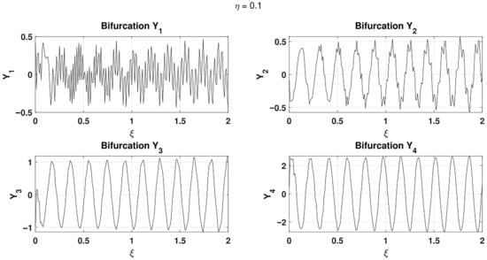
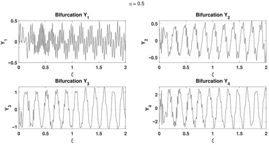
Figure 6. Bifurcation diagrams under the control parameter $\xi$ for $\eta =0.1,0.5$.

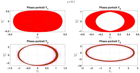
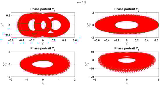
Figure 7. Phase portraits for different values of $\eta$ at $\xi =1$.

8. Conclusions

In conclusion, the present study modeled the deflection of waves over an elastic isotropic plate using a Pasternak-like nonlinear elastic foundation. A promising analytical method of examination has been proposed through the application of the modified extended tanh expansion method; moreover, a couple of ansatz function methods were deployed for validations and the construction of more solutions. The frequency equation of the linear model has been acquired and analyzed concerning the subsequent expressions for the phase and group velocities. The modulation instability spectrum has been acquired and examined, in addition to the establishment of bifurcation analysis of the overall dynamical system of the reduced differential equations. Further, some numerical results have been presented for clarity and justification of the proposed nonlinear model. Notably, it is concluded that an increase in both the Pasternak-like nonlinear parameter $\eta$ and time variation (for $x>0$) decreased the nonlinear deflection in the plate, while an increase in the stiffness of the Winkler foundation increased deflection in the medium. What is more, the study also notes that increasing the Winkler foundation stiffness increased the dispersion of nonlinear waves in the governing isotropic plate, while the presence of Pasternak-like nonlinear parameter decreased the dispersion of waves with an increase in the wave number. Equally, both the phase and group velocities are noted to be significantly affected, including the gain function of the modulation instability. Finally, taken together, phase portraits and bifurcation diagrams provided a complete framework for understanding the global dynamics of nonlinear systems, predicting regions of stability or instability, and characterizing complex phenomena such as limit cycles and chaotic attractors. In the end, this study provides a framework for a complete analysis of the dispersion of nonlinear waves in beams and plates, paramount structures arising in diverse engineering applications. In addition, this study will benefit a wide range of professions, including optical communication, nonlinear vibration, and fluid-solid interaction areas, among others.

References

- Ewing, W.M. Elastic Waves in Layered Media; McGraw Hill Book Company Inc.: New York, NY, USA, 1957. [Google Scholar]
- Daniel, I.M.; Ishai, O.; Daniel, I.M.; Daniel, I. Engineering Mechanics of Composite Materials; Oxford University Press: New York, NY, USA, 2006. [Google Scholar]
- Abd-Alla, A.M.; Abo-Dahab, S.M.; Khan, A. Rotational effects on magneto-thermoelastic Stoneley, Love, and Rayleigh waves in fibre-reinforced anisotropic general viscoelastic media of higher order. Comput. Mater. Contin 2017, 53, 49–72. [Google Scholar]
- Norris, A.N. Letters to the Editor: Flexural edge waves. J. S. Vib. 1994, 171, 571–573. [Google Scholar] [CrossRef]
- Kaplunov, J.; Nobili, A. The edge waves on a Kirchhoff plate bilaterally supported by a two-parameter elastic foundation. J. Vib. Control 2015, 23, 2014–2022. [Google Scholar] [CrossRef]
- Althobaiti, S.N.; Kaplunov, J.; Prikazchikov, D.A. An edge moving load on an orthotropic plate resting on a Winkler foundation. Precedia Eng. 2017, 199, 2579–2584. [Google Scholar] [CrossRef]
- Althobaiti, S.; Prikazchikov, D.A. The flexural edge waves of arbitrary profile in an orthotropic elastic plate. Proc. Natl. Acad. Sci. Armen. Mech. 2016, 69, 16–24. [Google Scholar]
- Althobaiti, S.; Hawwa, M.A. Flexural edge waves in a thick piezoelectric film resting on a Winkler foundation. Crystal 2022, 12, 640. [Google Scholar] [CrossRef]
- Kumari, T.; Som, R.; Althobaiti, S.; Manna, S. Bending waves at the edge of a thermally affected functionally graded poroelastic plate. Thin-Walled Struct. 2023, 186, 110719. [Google Scholar] [CrossRef]
- Wang, Y.H.; Tham, L.G.; Cheung, Y.K. Beams and plates on elastic foundations: A review. Prog. Struct. Eng. Mater. 2005, 7, 174–182. [Google Scholar] [CrossRef]
- Doyle, P.F.; Pavlovic, M.N. Vibration of beams on partial elastic foundations. Earthquake Eng. Struct. Dyn. 1982, 10, 663–674. [Google Scholar] [CrossRef]
- Zhou, D. A general solution to vibrations of beams on variable Winkler elastic foundation. Compos. Struct. 1993, 47, 83–90. [Google Scholar] [CrossRef]
- Schulze, S.H.; Pander, M.; Naumenko, K.; Altenbach, H. Analysis of laminated glass beams for photovoltaic applications. Int. J. Solids Struct. 2012, 49, 2027–2036. [Google Scholar] [CrossRef]
- Sayyad, A.S.; Ghugal, Y.M. Bending, buckling and free vibration of laminated composite and sandwich beams: A critical review of literature. Compos. Struct. 2017, 171, 486–504. [Google Scholar] [CrossRef]
- Sahin, O. Vibration of a composite elastic beam on an inhomogeneous elastic foundation. J. Appl. Math. Comp. Mech. 2020, 19, 107–119. [Google Scholar]
- Sahin, O.; Erbas, B.; Kaplunov, J.; Savsek, T. The lowest vibration modes of an elastic beam composed of alternating stiff and soft components. Arch. Appl. Mech. 2020, 90, 339–352. [Google Scholar] [CrossRef]
- Ebrahimi, F.; Seyfi, A. A wave propagation study for porous metal foam beams resting on an elastic foundation. Waves Random Complex Med. 2024, 34, 182–196. [Google Scholar] [CrossRef]
- Erbas, B.; Kaplunov, J.; Nobili, A.; Kilic, G. Dispersion of elastic waves in a layer interacting with a Winkler foundation. J. Acoust Soc. Am. 2018, 144, 2918–2925. [Google Scholar] [CrossRef]
- Mubaraki, A.M. Asymptotic consideration for Rayleigh waves on a coated orthorhombic elastic half-space reinforced by the elastic Winkler foundation. Math. Comput. Appl. 2023, 28, 109. [Google Scholar] [CrossRef]
- Fu, Y.B. Perturbation Methods and Nonlinear Stability Analysis; Cambridge University Press: Cambridge, MA, USA, 2009. [Google Scholar]
- Lenci, S.; Clementi, F. Flexural wave propagation in unilateral elastic foundation. Nonlinear Dyn. 2020, 99, 721–735. [Google Scholar] [CrossRef]
- Collet, B.; Pouget, J. Two-dimensional modulation and instabilities of flexural waves of a thin plate on nonlinear elastic foundation. Wave Mot. 1998, 27, 341–354. [Google Scholar] [CrossRef]
- Althobaiti, S.; Mubaraki, A.M.; Nuruddeen, I.R. Dispersion of flexural waves on an initially pre-stressed thin plate resting on nonlinear elastic foundations. Acta Mech. 2025, 236, 6141–6159. [Google Scholar] [CrossRef]
- Abdullah, E.H.; Zaghrout, A.A.; Ahmed, H.M.; Bahnasy, A.I.A.; Rabie, W.B. Soliton dynamics and travelling wave solutions for higher-order nonlinear Schrodinger equation in birefringent fibers using improved modified extended tanh method. Opt. Quant. Electron. 2024, 56, 1184. [Google Scholar] [CrossRef]
- Kudryashov, N.A. One method for finding exact solutions of nonlinear differential equations. Commun. Nonlinear Sci. Numer. Simul. 2012, 17, 2248–2253. [Google Scholar] [CrossRef]
- Rabie, W.B.; Ahmed, H.M.; Marin, M.; Syied, A.A.; Abd-Elmonem, A.; Abdallah, N.S.E.; Ismail, M.F. Thorough investigation of exact wave solutions in nonlinear thermoelasticity theory under the influence of gravity using advanced analytical methods. Acta Mech. 2025, 236, 1599–1632. [Google Scholar] [CrossRef]
- Abdelrahman, M.A.E.; Zahran, E.H.M.; Khater, M.M.A. The e−ψ(θ)-expansion method and its application for solving nonlinear evolution equations. Int J. Mod. Nonlinear Theory Appl. 2015, 4, 37–47. [Google Scholar] [CrossRef]
- Rizvi, S.T.R.; Seadawy, A.R.; Farah, N.; Ahmad, S.; Althobaiti, A. The interactions of dark, bright, parabolic optical solitons with solitary wave solutions for nonlinear Schrodinger-Poisson equation by Hirota method. Opt. Quant. Electron. 2024, 56, 1162. [Google Scholar] [CrossRef]
- Nass, A.M. Lie symmetry analysis and exact solutions of fractional ordinary differential equations with neutral delay. Appl. Math. Comput. 2019, 347, 370–380. [Google Scholar] [CrossRef]
- Al Qarni, A.A.; Bodaqah, A.M.; Mohammed, A.S.H.F.; Alshaery, A.A.; Bakodah, H.O.; Biswas, A. Dark and singular cubic-quartic optical solitons with Lakshmanan-Porsezian-Daniel equation by the improved Adomian decomposition scheme. Ukrainian J. Phys. Opt. 2023, 24, 46. [Google Scholar] [CrossRef]
- Wazwaz, A.M. A variety of optical solitons for nonlinear Schrodinger equation with detuning term by the variational iteration method. Optik 2019, 196, 163169. [Google Scholar] [CrossRef]
- Yomba, E. A generalized auxiliary equation method and its application to nonlinear Klein-Gordon and generalized nonlinear Camassa-Holm equations. Phys. Let. A 2008, 372, 1048–1060. [Google Scholar] [CrossRef]
- Muhammad, S.; Althobaiti, A.; Nuruddeen, R.I.; Sambo, H.S.; Kim, H. Application of guaranteeing analytical methods in the construction of optical structures for nonlinear Schrodinger equations. Mod. Phys. Lett. A 2025, 40, 2550189. [Google Scholar] [CrossRef]
- Demirbilek, U.; Danladi, A.; Bulut, H.; Seadawy, A.R.; Ahmed, K.K. Exploring optical solitons, modulation instability and chaotic behavior in the Schrodinger-Hirota equation. Rend. Fis. Acc. Lincei 2025, 36, 1093–1108. [Google Scholar] [CrossRef]
- Songong, E.F. Nonlinear Vibration of Beams and Plates Resting on Elastic Foundations Having Nonlinear Stiffness Properties. Ph.D. Thesis, University of Cape Town, Cape Town, South Africa, 2023. Available online: http://hdl.handle.net/11427/39424 (accessed on 6 November 2025).
- Lee, C.; Hwang, Y.G.; Jang, T.S. Application of pseudo-parameter iteration method to nonlinear deflection analysis of an infinite beam cross-sections on a nonlinear elastic foundation. Heliyon 2024, 10, e28176. [Google Scholar] [CrossRef] [PubMed]
- Malikan, M.; Eremeyev, V.A. On nonlinear bending study of a piezo-flexomagnetic nanobeam based on an analytical-numerical solutions. Nanomaterials 2020, 10, 1762. [Google Scholar] [CrossRef] [PubMed]
- Seadawy, A.R.; Nuruddeen, R.I.; Aboodh, K.S.; Zakariya, Y.F. On the exponential solutions to three extracts from extended fifth-order KdV equation. J. King Saud Univ. Sci. 2019, 32, 765–769. [Google Scholar] [CrossRef]
- Selim, M.M.; Althobaiti, S. Longitudinal vibration of defected single-layer nanoplate using nonlocal elasticity theory. Contemp. Math. 2025, 6, 8794. [Google Scholar] [CrossRef]
- Li, Q.; Han, Y.; Guo, B. A critical Kirchhoff problem with a logarithmic type perturbation in high dimension. Commun. Anal. Mech. 2024, 16, 578–598. [Google Scholar] [CrossRef]
- Arora, R.; Fiscella, A.; Mukherjee, T.; Winkert, P. On double phase Kirchhoff problems with singular nonlinearity. Adv. Nonlinear Anal. 2023, 12, 20220312. [Google Scholar] [CrossRef]
- Lv, W. Ground states of a Kirchhoff equation with the potential on the lattice graphs. Commun. Anal. Mech. 2023, 15, 792–810. [Google Scholar] [CrossRef]
- Shibata, T. Bifurcation diagrams of one-dimensional Kirchhoff-type equations. Adv. Nonlinear Anal. 2023, 12, 356–368. [Google Scholar] [CrossRef]
- Qawaqneh, H.; Manafian, J.; Alharthi, M.; Alrashedi, Y. Stability analysis, modulation instability, and beta-time fractional exact soliton solutions to the Van der Waals equation. Mathematics 2024, 12, 2257. [Google Scholar] [CrossRef]
- Demirbilek, U.; Tedjani, A.H.; Seadawy, A.R. Analytical solutions of the combined Kaitat II-X equation: A dynamical perspective on bifurcation, chaos, energy, and sensitivity. AIM Math. 2025, 10, 13664–13691. [Google Scholar] [CrossRef]
- Yao, S.-W.; Tariq, K.U.; Inc, M.; Tufail, R.N. Modulation instability analysis and soliton solutions of the modified BBM model arising in dispersive medium. Rest. Phy. 2023, 46, 106274. [Google Scholar] [CrossRef]
- Luo, A.C.J. Bifurcation and Stability in Nonlinear Dynamical Systems; Springer: Cham, Switzerland, 2020. [Google Scholar]
- Khalil, H.K. Nonlinear Systems, 4th ed.; Prentice Hall: Saddle River, NJ, USA, 2022. [Google Scholar]
- Chen, X. Dynamical systems of differential equations based on information technology: Effects of integral step size on bifurcation and chaos control of discrete Hindmarsh-Rose models. Mobile Inf. Syst. 2022, 1, 1425403. [Google Scholar] [CrossRef]
- Aguirre, P.; Hong, Y.; Wang, Y. Recent advances in bifurcation analysis: Theory and applications. Front. Appl. Math. Stat. 2022, 8, 893759. [Google Scholar] [CrossRef]
- Chahlaoui, Y.; Ali, A.; Ahmad, J.; Javed, S. Dynamical behavior of chaos, bifurcation analysis and soliton solutions to a Konno-Onno model. PLoS ONE 2023, 18, e0291197. [Google Scholar] [CrossRef] [PubMed]
- Kato, K.; Itoh, Y.; Kousaka, T. Predicting bifurcation points using machine-learning-assisted time-series reconstruction. Int. J. Bifur. Chaos 2025, 35, 1–15. [Google Scholar]
- Allogmany, R.; Sarrah, A.; Abdoon, M.A.; Alanazi, F.J.; Berir, M.; Alharbi, S.A. A comprehensive analysis of complex dynamics in the fractional-order Rossler system. Mathematics 2025, 13, 3089. [Google Scholar] [CrossRef]
Disclaimer/Publisher’s Note: The statements, opinions and data contained in all publications are solely those of the individual author(s) and contributor(s) and not of MDPI and/or the editor(s). MDPI and/or the editor(s) disclaim responsibility for any injury to people or property resulting from any ideas, methods, instructions or products referred to in the content. |
© 2025 by the authors. Licensee MDPI, Basel, Switzerland. This article is an open access article distributed under the terms and conditions of the Creative Commons Attribution (CC BY) license.