Bifurcation Geometry, Global Stability, and Nonlinear Nematicon Dynamics of the Generalized Hunter–Saxton Model

Abstract

This study examines the generalized nonlinear Hunter–Saxton (HS) model: ${\Phi }_{tx}=\Phi {\Phi }_{xx}+\gamma {\Phi }_x^2,\gamma \ne 0,$ that describes the evolution of spatial potential and angular velocity in the vector field of nematic liquid crystals. Closed-form nematicons are derived via the order reduction of the traveling wave ODE. The qualitative structures are analyzed for different values of the nonlinear parameter $\gamma$. The solutions are graphically depicted to discover rich nematicon geometries including parabolic, cuspon, kink, and singular wave structures. A comprehensive dynamic analysis of the reduced nonlinear ordinary system is performed using the phase plane method, which helps to reveal the non-isolated continuity of equilibrium and the role of singular manifolds in shaping the system’s sensitivity and stability. Bifurcation cases are investigated for distinct values of $\gamma$, and various transitions in trajectory geometry and semi-stability features are shown. The novelty appears in the comprehensive integrating of analytic and dynamic characterizations, through global phase and bifurcation analysis, of the generalized HS equation (HSE), which uncovers the control of nonlinear coefficient $\gamma$ in governing the geometry and stability of the nematicons. Also, the analysis confirms the non-chaotic nature of the associated two-dimensional system, compatible with the Poincaré–Bendixson theorem.

1. Introduction

The Hunter–Saxton equation (HSE) was initially designed to asymptotically model the propagation of weak nonlinear waves in the orientation domains of massive nematic liquid crystals. The formal (1+1)-dimensional HSE, that represents the non-linear and non-perturbed evolution of gradients in the director orientation, is derived to be [1]

$${\Phi }_{tx}=\Phi {\Phi }_{xx}+\frac{1}{2}{\Phi }_x^2,$$

(1)

where $\varphi (x,t)$ represents the direction of local orientation in a one-dimensional nematic liquid crystal.

The equation allows for gradient inflation over a finite time, where ${\Phi }_x$ becomes infinite while $\Phi$ remains continuous [2]. This mechanism is closely related to the geometric nature of the equation, which can be interpreted as geodesic flow in homogeneous space [3]. A continuous semi-group of weak dissipative solutions to Equation (1) was constructed by Bressan and Constantin [4]. The HSE is also related to the Camassa–Holm equation with a shortwave asymptotic limit, further solidifying its place within the broader theory of integrated shallow-water models and directing field models [5]. Global and conservative unique solutions on a line for the Cauchy-type HSE were proved in [6]. Accordingly, the Lie symmetry analysis is employed to obtain the corresponding conservation laws [7]. Numerical solutions of the considered model were achieved using the exponential cubic B-spline collocation [8], Hosoya polynomial [9], and cell average-based neural network methods [10]. The generalized characteristics method has been employed to derive numerical $\alpha$-dissipative solutions to the initial-valued HSE [11]. See also the listed references therein.

The generalized version of the HSE Equation (1) is given as follows [12]:

$${\Phi }_{tx}=\Phi {\Phi }_{xx}+\gamma {\Phi }_x^2,\gamma \ne 0.$$

(2)

The non-linear parameter $\gamma$ influences the qualitative shape, strength, and type of the traveling wave solutions. If $\beta \ne 1/2$, Equation (2) models the Einstein–Weil geometry structure [12,13]. $\Phi (x,t)$ represents the spatial potential angular velocity in the liquid crystal’s directional field. The generalized form Equation (2) preserves integrability and allows Lax pairs and iteration operators [2,14]. Weak solutions and frameworks have been developed for energy acceptance in both conservative and dissipative environments [2]. Numerical processing of the generalized Hunter–Saxton model Equation (2) due to a sinc collocation approach along with the $\theta$-weighted method was conducted by Ahmad et al. [15].

Since this topic has not been thoroughly discussed to our knowledge, the present analysis addresses the mathematical effect of the nonlinear coefficient $\gamma$ on the structure and stability of traveling wave solutions. We precisely determine how variations in $\gamma$ affect the existence, qualitative geometry, and global stability of nematicons (spatial optical solitons in nematic liquid crystals [16]) through precise reduction and nonlinear dynamical analysis.

In what follows, Section 2 presents a traveling wave reduction and derives exact closed-form solutions. Section 3 provides graphical illustrations of the resulting wave profiles. Section 4 develops a qualitative dynamical analysis, including phase plane structure, sensitivity, stability, and bifurcation behavior. Section 5 concludes the paper and outlines directions for future work.

2. Mathematical Analysis

Applying the traveling wave transformation $\zeta =\kappa x-\nu t$, $\kappa \ne 0$ and $\nu \ne 0$ is the wave speed constant in Equation (2), and transforms it into the following nonlinear ordinary differential equation (NODE):

$$-\kappa \left({\varphi }^{″}\left(\zeta \right)(\kappa \varphi \left(\zeta \right)+\nu )+\gamma \kappa {\varphi }^{\prime }{\left(\zeta \right)}^2\right)=0,$$

(3)

where $\Phi (x,t)=\varphi \left(\zeta \right)$.

Equation (3) is classified as $\zeta$-independent, so it is solvable. For $\kappa \ne 0$, assuming that

$$F\left(\varphi \right)={\varphi }^{\prime }\left(\zeta \right)\Rightarrow {\varphi }^{″}\left(\zeta \right)=F\left(\varphi \right)F^{\prime }\left(\varphi \right).$$

Substituting into Equation (3), and solving the obtained separated variables’ first-order NODE gives:

$${\displaystyle \frac{d\varphi }{d\zeta }}=C_1{(\kappa \varphi +\nu )}^{-\gamma }.$$

(4)

Solving for $\varphi \left(\zeta \right)$ and by backward substitution, the exact solutions of Equation (2) are

$$\Phi (x,t)={\displaystyle \frac{C_2{e}^{C_1\kappa (\kappa x-\nu t)}-\nu }{\kappa }},if\gamma =-1,$$

(5)

and,

$$\Phi (x,t)={\displaystyle \frac{{\left(C_1(\kappa x-\nu t)+C_2\right)}^{\frac{1}{\gamma +1}}-\nu }{\kappa }},if\gamma \ne -1,$$

(6)

where $C_i$ is the arbitrary constant of integration.

The general solution to this equation is algebraic when $\gamma \ne -1$ and exponential when $\gamma =-1$, and is therefore monotonic or exponential on its domain of definition. Consequently, the solution cannot be bounded or oscillatory, thus excluding the existence of nontrivial periodic real solutions for the traveling waves. Furthermore, applying The ansatz-trigonometric [17] and hyperbolic methods [18] to Equation (3) yields only trivial constant solutions. Therefore, the generalized Hunter–Saxton equation does not admit any non-trivial periodic or hyperbolic traveling wave solutions.

3. Illustrations

Graphical representations of the obtained traveling wave solutions (Equations (5) and (6)) are presented for different values of parameter $\gamma$. In all cases the integration’s constants $C_1$ and $C_2$ are assumed to be one. Also, the domains are chosen to clearly show the wave flow in each case.

Figure 1 shows the exponential growth, as the space x increases and time t vanishes, of the molecular angular velocity $\Phi (x,t)$ in Equation (5) with suitable parameters $\kappa =\nu =1$. It can also be used to study the angular velocity behavior of the director field.

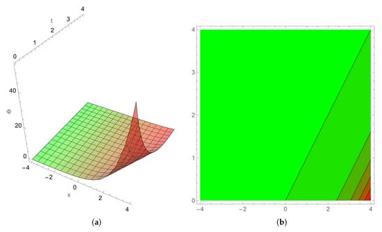
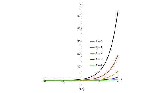
Figure 1. The potential spatial angular velocity (a) 3D semi-kink nematicon, the (b) corresponding contour plot, and (c) 2D profiles for $\gamma =1$ and $t\in \left\{0,2,\dots ,8\right\}$.

For $\kappa =\nu =1$ in Equation (6), the singular spatial potential angular velocity with $\gamma =-2$ is depicted in Figure 2. Figure 3 represents the corresponding angular velocity which is the most significant variable in the nematic liquid crystal interpretation.

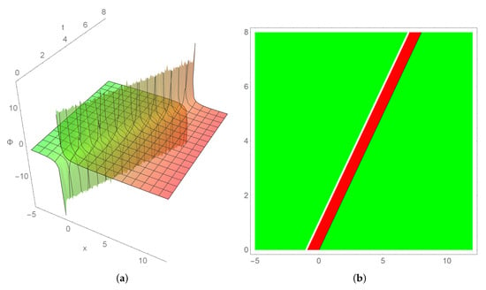
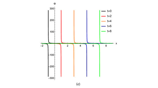
Figure 2. The potential spatial angular velocity. (a) 3D singular-kink nematicon, (b) the corresponding contour plot, and (c) 2D profiles for $\gamma =-2$ and $t\in \left\{0,2,\dots ,8\right\}$.

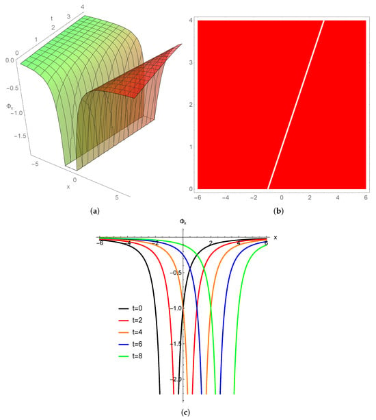
Figure 3. The angular velocity (a) 3D parabolic nematicon, the (b) corresponding contour plot, and (c) 2D profiles for $\gamma =-2$ and $t\in \left\{0,2,\dots ,8\right\}$.

For $\gamma =-0.5$, Figure 4 and Figure 5 show the steady state of the spatial potential angular velocity ($\Phi$) and the director alignment strain (${\Phi }_x$) in Equation (6), respectively.

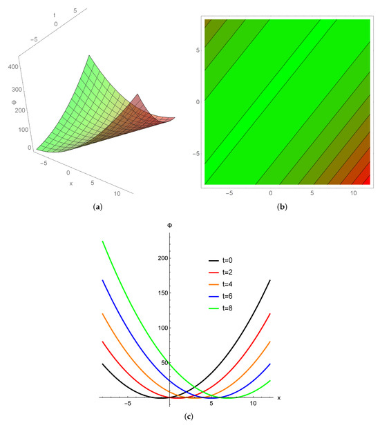
Figure 4. The potential spatial angular velocity. (a) 3D parabolic nematicon, the (b) corresponding contour plot, and (c) 2D profiles for $\gamma =-0.5$ and $t\in \left\{0,2,\dots ,8\right\}$.

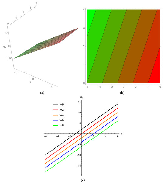
Figure 5. The angular velocity. (a) 3D oblique linear nematicon, (b) the corresponding contour plot, and (c) 2D profiles for $\gamma =-0.5$ and $t\in \left\{0,2,\dots ,8\right\}$.

In Figure 6, for $\gamma =2$, we illustrate the spatial growth possibilities of angular velocity in a cuspon-type nematicon (the soliton in liquid crystal case [19]). The corresponding increasing oblique nematicon of angular velocity is shown in Figure 7.

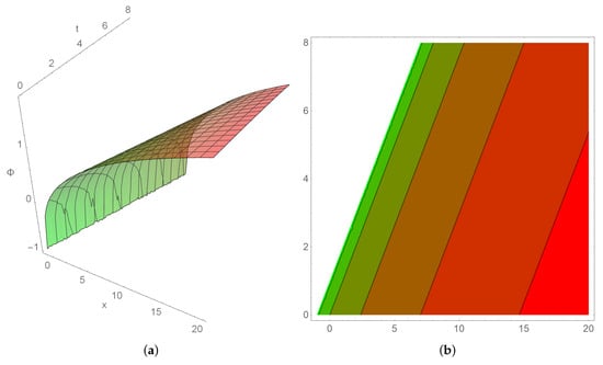
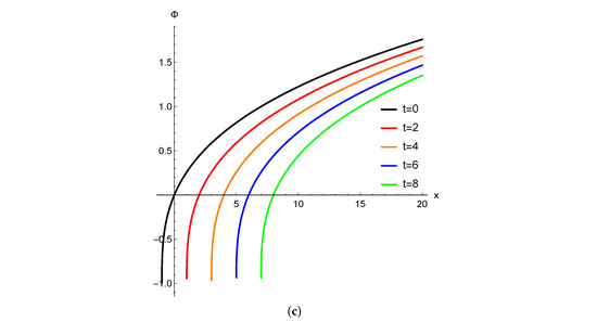
Figure 6. The potential spatial angular velocity. (a) 3D cuspon nematicon, (b) the corresponding contour plot, and (c) 2D profiles for $\gamma =2$ and $t\in \left\{0,2,\dots ,8\right\}$.

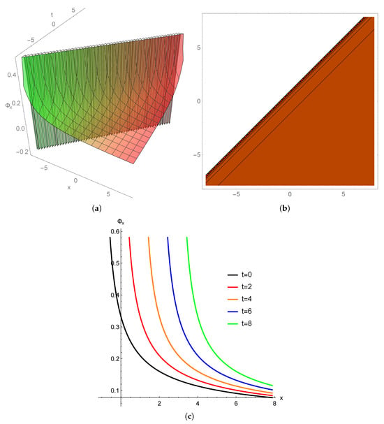
Figure 7. The angular velocity (a) 3D cuspon nematicon, the (b) corresponding contour plot, and (c) 2D profiles for $\gamma =2$ and $t\in \left\{0,2,\dots ,8\right\}$.

4. Dynamical Analysis

In parallel to previous works [17,20,21], this part focuses on studying the qualitative characteristics of the reduced NODE Equation (3). The analysis includes the sensitivity to initial data, stability near stationary points, and possibility of chaotic conductance.

The model under study Equation (3) can be formulated as a couple of first-order NODEs:

$${\displaystyle \frac{d\varphi }{d\zeta }}=\psi ,{\displaystyle \frac{d\psi }{d\zeta }}=-{\displaystyle \frac{\gamma \kappa }{\kappa \varphi +\nu }}{\psi }^2.$$

(7)

Here, $\varphi \left(t\right)$ and $\psi \left(t\right)$ are state variables that illustrate angular displacement and velocity, respectively. The set of equilibrium (stationary) points is the entire $\varphi$-axis. i.e., the set $\left\{\right(z,0):z\in \mathbb{R}\}$. The vertical line $\varphi =(-\nu /\kappa ,0)$ represents the singular line in the $\varphi \psi$-plane (phase plane). As the line $\psi =0$ consists of all stationary solutions, the velocity vanishes on it, and the solutions stay constant.

4.1. The Phase Plane Method

The phase plane method is a useful technique used to qualitatively analyses systems of NODEs by examining the curves of their solutions in the $\varphi \psi$-plane rather than dealing with time t. The phase plane technique is a helpful technique that allows to understand the global behavior of the solutions, visualize the motion in the $\varphi \psi$-plane, analyze solutions near critical stationary points, and classify each critical point. Even when linearization is insufficient or the starting data is far from stationary, the phase plane profile still provides worthy information [22] (p. 384).

Sequentially, the system in Equation (7) can be expressed as

$${\displaystyle \frac{d\varphi }{d\psi }}=-{\displaystyle \frac{\kappa \varphi +\nu }{\gamma \kappa \psi }}.$$

(8)

Solving the obtained separated-variables NODE gives

$$\psi =C{(\kappa \varphi +\nu )}^{-\gamma },C\in \mathbb{R}.$$

(9)

Equation (9) shows the solutions shapes in the phase plane. That is, the solution curves satisfy a conserved quantity (each solution path lies on one of those curves). Also, we can obtain that the solution curve $\varphi$ remains constant while the velocity $\psi =0$.

4.2. Sensitivity Dynamics

Dynamical systems are typically characterized by their sensitivity to initial conditions, model parameters, and perturbation tools. Small initial changes may cause diverge trajectories over long-time (which is linearly related to the space $\zeta$ through traveling wave transformation in Section 2). The sensitivity conducts to understand the system’s evolution depending on the parameter $\gamma$.

For $\kappa =\nu =1$, the numerical simulations through the Runge–Kutta method of the fourth order (RK4), and with the aid of Mathematica package 11, are shown in Figure 8 for $\gamma =1$ and Figure 9 for $\gamma =-1$. The initial positions and velocities are chosen at the points $P_1=(\varphi \left(0\right)=0,\psi \left(0\right)=0.01)$, $P_2=(0,0.015)$, and $P_3=(0,0.02)$ near the pole.

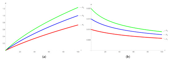
Figure 8. The (a) displacement and (b) velocity trajectories in Equation (7) near the origin for $\gamma =1$.

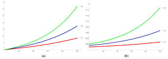
Figure 9. The (a) displacement and (b) velocity trajectories in Equation (7) near the origin for $\gamma =-1$.

In Figure 10 and Figure 11, we plot the comparison of displacements $\varphi \left(\zeta \right)$, part $\left(a\right)$, and corresponding velocities $\psi \left(\zeta \right)$, part $\left(b\right)$, for $\gamma =1,-0.5$, respectively, near the singular line $\varphi =-1$. The starting values are $P_1=(\varphi \left(0\right)=-0.99,\psi \left(0\right)=0.01)$, $P_2=(-0.99,0.015)$, and $P_3=(-0.99,0.02)$.

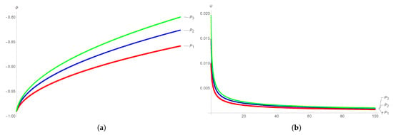
Figure 10. The (a) displacement and (b) velocity trajectories in Equation (7) near the singular line for $\gamma =1$.

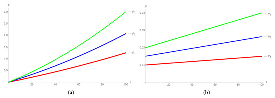
Figure 11. The (a) displacement and (b) velocity trajectories in Equation (7) near the singular line for $\gamma =-0.5$.

The figures illustrate how small perturbations in the initial values gradually cause a marked divergence in the evolution of the displacement trajectories $\varphi \left(\zeta \right)$. This demonstrates the system’s long-term memory and expansion behavior, and leads to potential instability.

For positive $\gamma$, Figure 8 and Figure 10, the velocity $\psi \left(t\right)$ converges smoothly. The results confirm the stabilizing effect of a positive $\gamma$ on the velocity, which remains smooth and controlled. For a negative $\gamma$, the divergence of the velocity paths becomes rapid and uncontrolled, indicating potential instability, as in the case of displacement. That is, the results confirm the potential instability as illustrated in Figure 9 and Figure 11.

4.3. Bifurcation Dynamics

As mentioned before, the system in Equation (7) possesses equilibria on line of non-isolated stationary points $\left\{\right(z,0):z\in \mathbb{R},z\ne -\nu /\kappa \}$ (one-dimensional manifold of fixed points). The linearization algorithm produces the following nilpotent Jacobian matrix:

$$J\left(z,0\right)=\left(\begin{array}{cc}0& 1\\ 0& 0\end{array}\right).$$

This implies the linearization decadence of the nonlinear system, while it is critically stable (non-hyperbolic) for the corresponding linear system. In this situation, the equilibrium manifold acts as a center manifold, and the system exhibits critical (neutral) stability along the equilibrium direction.

Based on the above, the qualitative behavior of the nonlinear system Equation (7) will be established through the phase plane solution Equation (9). Without loss of generality, the phase portraits of our system are considered with a choice of parameters $\kappa =\nu =1$.

For $\gamma <0$, the corresponding phase plane trajectories are plotted in Figure 12 with $\gamma =-2,-1$ and $-0.5$. The behavior near the singular line $\varphi =-\nu /\kappa =-1$ (red vertical line) shows parabolic tangents as $\gamma =-2$, straight lines pass through the singular point $(-1,0)$ with different slopes as $\gamma =-1$, and cusps (of the square root type) as $\gamma =-0.5$. Invariant phase curves for several values of C in Equation (9) are included to clearly show the path of these curves. The trajectories vanish near the singular line, approach the equilibrium form from one side, and alienate from the other. In such case, semi-stability occurs.

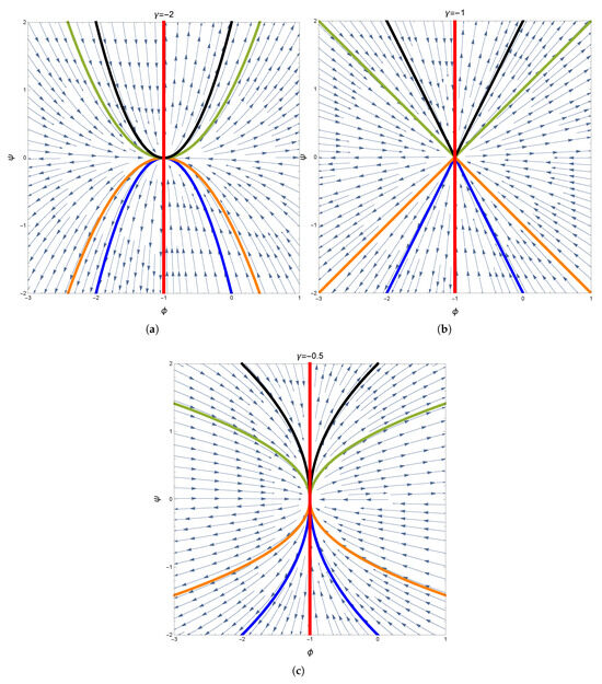
Figure 12. The phase portraits for different values of (a) $\gamma$ = −2, (b) $\gamma$ = −1, and (c) $\gamma$ = −0.5. The red vertical line is the singular line; blue arrows represent the vector field. Continuous colored curves represent the solution in Equation (9) with C = −2 (blue), C = −1 (orange), C = 1 (black), and C = 2 (green).

On the other hand, for $\gamma >0$, Figure 13 shows the semi-stability for $\gamma =0.5,1$ and 2. The trajectories diverge at the singular line and decay to the equilibrium away from it. The blow-up is directly relative with the magnitude of parameter $\gamma$. The case $\gamma =0.5$ represents a conservative blow-up, while $\gamma =1$ and $\gamma =2$ correspond to hyperbolic and strong diverges, respectively.

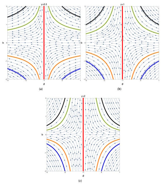
Figure 13. The phase portraits for different values of (a) $\gamma$ = 0.5, (b) $\gamma$ = 1, and (c) $\gamma$ = 2. The red vertical line is the singular line; blue arrows represent the vector field. Continuous colored curves represent the solution in Equation (9) with C = −2 (blue), C = −1 (orange), C = 1 (black), and C = 2 (green).

Changes in $\gamma$ and the related curvature of phase trajectories illustrate the bifurcation in the trajectories’ geometry. This comparison clarifies a bifurcation situations obtained by the variance of $\gamma$. The phase trajectories switch from closing to at the singular line for $\gamma <0$ to blowing up for $\gamma >0$. Hence, the parameter $\gamma$ governs both the local geometry near the singular line and the global stability behavior, playing a crucial role in the qualitative analysis and in the efficiency of numerical solvers.

Finally, the neutral stability occurs when $\gamma =0$. Figure 14 shows the trajectories in horizontal straight lines. In this case, the system undergoes degenerate manifold bifurcation, comparable to a trans-critical bifurcation along an entire curve of stationary points.

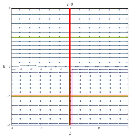
Figure 14. The phase portrait for $\gamma =0$. The red vertical line is the singular line; blue arrows represent the vector field. Continuous colored curves represent the solution in Equation (9) with C = −2 (blue), C = −1 (orange), C = 1 (black), and C = 2 (green).

In summary, The transverse stability of an equilibrium manifold is entirely governed by nonlinearities. Phase plane analysis shows that the trajectories may approach the equilibrium line from one side while diverging from the other, resulting in semi-stability, or may remain neutrally stable depending on the value of the nonlinear coefficient $\gamma$. Thus, the stability of the system is not determined locally by eigenvalues, but globally by the geometry of the invariant curves and the presence of the singular manifold.

4.4. Chaotic Dynamics

The system is two-dimensional and autonomous, and according to the Poincaré–Bendixson theorem ([23]; Theorem 16.2, p. 389), neither periodic nor chaotic trajectories exist. All trajectories either converge, diverge, or transition neutrally. Therefore, the system demonstrates non-oscillatory and non-chaotic dynamics.

5. Conclusions and Future Work

This study presents an analytic/dynamic framework for the generalized Hunter–Saxton equation, which simulates the evolution of orientation and angular velocity in one-dimensional nematic liquid crystals. traveling wave reductions produce closed-form parabolic, cuspon, kink, and singular nematic solutions, and correspond to distinct modes of director field deformation. These features provide explicit descriptions of local and singular orientation patterns that may arise in nematic media under the influence of nonlinear elastic effects.

Nonlinear dynamical analysis reveals that the reduced system possesses a continuum of equilibrium states representing uniform wave alignment, as well as a singular manifold associated with critical orientation gradients. Physically, a singular structure represents a limit beyond which the angular velocity increases dramatically, leading to strong distortions in the liquid crystal. This behavior cannot be observed by linear analysis, indicating that the system becomes highly nonlinear near these stationary conditions.

Changes in the nonlinear coefficient $\gamma$ were shown to directly regulate the physical response of the system. Positive values of $\gamma$ lead to smoothing and controlled evolution of the angular velocity, consistent with stabilizing elastic interactions, while negative values promote rapid growth and sensitivity to disturbances, indicating physically unstable alignment systems. Therefore, the observed bifurcation scenarios represent transitions between distinct physical deformation mechanisms in the nematic structure.

Finally, the model is shown to exhibit no chaotic motion, in agreement with the Poincaré–Bendixson theorem, highlighting the necessity of nonlinear analytical and numerical approaches when studying degenerate wave systems. This work therefore provides a solid analytical and dynamical basis for extending the Hunter–Saxton framework to more general settings, including higher-dimensional, fractional-order, and dissipative models of nematic liquid crystals.

References

- Hunter, J.K.; Saxton, R. Dynamics of director fields. SIAM J. Appl. Math. 1991, 51, 1498–1521. [Google Scholar] [CrossRef]
- Hunter, J.K.; Zheng, Y. On a completely integrable nonlinear hyperbolic variational equation. Physical D 1994, 79, 361–386. [Google Scholar] [CrossRef]
- Lenells, J. The Hunter–Saxton equation: A geometric approach. SIAM J. Math. Anal. 2008, 40, 266–277. [Google Scholar] [CrossRef]
- Bressan, A.; Constantin, A. Global solutions of the Hunter–Saxton equation. SIAM J. Math. Anal. 2005, 37, 996–1026. [Google Scholar] [CrossRef]
- Cotter, C.J.; Deasy, J.; Pryer, T. The r-Hunter–Saxton equation: Smooth and singular solutions and their approximation. Nonlinearity 2020, 33, 7016–7039. [Google Scholar] [CrossRef]
- Grunert, K.; Holden, H. Uniqueness of conservative solutions for the Hunter–Saxton equation. Res. Math. Sci. 2022, 9, 19. [Google Scholar] [CrossRef]
- Kakuli, M.C.; Sinkala, W.; Masemola, P. Conservation laws and symmetry reductions of the Hunter–Saxton equation via the double reduction method. Math. Comput. Appl. 2023, 28, 92. [Google Scholar] [CrossRef]
- Thube, N.H.; Lodhi, R.K. Numerical solution of Hunter–Saxton type equation via exponential cubic B-spline collocation method. Bound. Value Probl. 2025, 2025, 156. [Google Scholar] [CrossRef]
- Nirmala, A.; Kumbinarasaiah, S. Numerical solution of nonlinear Hunter–Saxton, Benjamin–Bona–Mahony, and Klein–Gordon equations using Hosoya polynomial method. Results Control Optim. 2024, 14, 100388. [Google Scholar] [CrossRef]
- Zhang, C.; Qiu, C.; Zhou, X.; He, X. Cell-average based neural network method for Hunter–Saxton equations. Adv. Appl. Math. Mech. 2024, 16, 833–859. [Google Scholar] [CrossRef]
- Christiansen, T.; Grunert, K.; Nordli, A.; Solem, S. A convergent numerical algorithm for α-dissipative solutions of the Hunter–Saxton equation. J. Sci. Comput. 2024, 99, 14. [Google Scholar] [CrossRef]
- Tod, K.P. Einstein–Weyl spaces and third-order differential equations. J. Math. Phys. 2000, 41, 5572–5581. [Google Scholar] [CrossRef]
- Dryuma, V. Applications of Riemannian and Einstein–Weyl geometry in the theory of second-order ordinary differential equations. Theor. Math. Phys. 2001, 128, 845–855. [Google Scholar] [CrossRef]
- Morozov, O.I. Integrability structures of the generalized Hunter–Saxton equation. Anal. Math. Phys. 2021, 11, 50. [Google Scholar] [CrossRef]
- Ahmad, I.; Ilyas, H.; Kutlu, K.; Anam, V.; Hussain, S.I.; Guirao, J.L.G. Numerical computing approach for solving Hunter–Saxton equation through sinc collocation method. Heliyon 2021, 7, e07600. [Google Scholar] [CrossRef]
- Assanto, G.; Peccianti, M.; Conti, C. Nematicons: Optical spatial solitons in nematic liquid crystals. Opt. Photonics News 2003, 14, 44–48. [Google Scholar] [CrossRef]
- Az-Zo’bi, E.A.; Hussain, E.; Iqbal, M.; Alomari, M.; Shah, A.; Yaro, D.; Aljawi, S.; Alsubaie, A.S.; Tashtoush, M.A. Chaotic and soliton dynamics of the nonlinear coupled Konno–Oono system in a magnetic field. AIP Adv. 2025, 15, 095101. [Google Scholar] [CrossRef]
- Hassaballa, A.A.; Gumma, E.A.E.; Adam, A.M.A.; Hamed, O.M.A.; Satty, A.; Salih, M.; Abdalla, F.A.; Mohammed, Z.M.S. Exact analytical solutions of the STFKS equation using Tanh–Coth and HSI methods. Front. Appl. Math. Stat. 2025, 11, 1568757. [Google Scholar] [CrossRef]
- Altawallbeh, Z.; Az-Zo’bi, E.; Alleddawi, A.O.; Senol, M.; Akinyemi, L. Novel liquid crystal model and its nematicons. Opt. Quantum Electron. 2022, 54, 795. [Google Scholar] [CrossRef]
- Al Zubi, M.A.; Afef, K.; Az-Zo’bi, E.A. Assorted spatial optical dynamics of a generalized fractional quadruple nematic liquid crystal system. Symmetry 2024, 16, 778. [Google Scholar] [CrossRef]
- Qiao, C.; Long, X.; Yang, L.; Zhu, Y.; Cai, W. Dynamical substitute for the Earth–Moon system via Hamiltonian analysis. Astrophys. J. 2025, 991, 46. [Google Scholar] [CrossRef]
- Zill, D.G.; Cullen, M.R. Differential Equations with Boundary-Value Problems, 7th ed.; Brooks/Cole Cengage Learning: Belmont, CA, USA, 2009. [Google Scholar]
- Coddington, E.A.; Levinson, N. Theory of Ordinary Differential Equations; Krieger: Malabar, FL, USA, 1984. [Google Scholar]
Disclaimer/Publisher’s Note: The statements, opinions and data contained in all publications are solely those of the individual author(s) and contributor(s) and not of MDPI and/or the editor(s). MDPI and/or the editor(s) disclaim responsibility for any injury to people or property resulting from any ideas, methods, instructions or products referred to in the content. |
© 2025 by the author. Licensee MDPI, Basel, Switzerland. This article is an open access article distributed under the terms and conditions of the Creative Commons Attribution (CC BY) license.