A Stochastic Formulation for the Dig-Limit Definition Problem in Short-Term Mine Planning Under Grade Uncertainty

Abstract

Uncertainty in short-term grade estimations can significantly affect destination policies and dig-limit definitions in open-pit mining. However, most dig-limit techniques still rely on deterministic methods and manual procedures. This study proposes a stochastic optimization model for the dig-limit definition problem that incorporates geological uncertainty through multiple grade scenarios and explicitly controls deviations from production targets. Two real case studies were evaluated to compare the stochastic formulation against deterministic and manual definitions. Results show that the stochastic model systematically improves economic performance, with profit increases of up to 2.3% over deterministic policies and up to 4.3% when compared against manual solutions. The stochastic solution also reduces deviations from metal and grade targets, producing more stable outcomes across scenarios. The model is computationally efficient, with solution times below 25 s for all case studies, which are compatible with practical short-term planning workflows. Overall, our findings demonstrate that incorporating grade variability into the dig-limit definition improves profitability and reliability in short-term mine planning horizons.

1. Introduction

Open-pit mining is the most widely used mining method globally, accounting for more than 80% of total metal production [1]. In this method, ore is extracted from the surface through a series of horizontal layers known as benches [2]. Each bench contains different types of materials: high-grade ore, which is typically sent to the processing plant; low-grade or marginal ore, which is commonly stockpiled for future use; and waste material, which is disposed of in waste dumps. The large scale of open-pit operations often requires many years to fully exploit a deposit, giving rise to several key strategic decisions. One of the most fundamental is determining the final limits of the excavation, known as the final-pit problem. This decision is critical, as it defines the portion of the orebody that will be considered economically viable for extraction [3,4,5]. Another essential decision is the extraction sequence within the final pit, which directly influences the net present value (NPV) of the project, which is one of the most commonly used economic indicators for assessing the viability of a mining operation [6,7,8]. In this work, we focus on another key decision at shorter planning horizons: the operational definition of material destinations, referred to as the dig-limit definition, which operationalizes the extraction sequence [9,10,11].

Given the importance of these decisions in determining the economic and operational feasibility of mining projects, Operations Research has become a vital tool for supporting planners across the mineral value chain. An extensive body of literature has addressed the most prominent problems in open-pit mine planning, offering mathematical formulations and solution strategies that are now widely used in the mining industry [3,6,12,13,14,15]. For example, the final-pit problem has been formulated as an integer program that maximizes the economic value of extracting individual blocks while satisfying geotechnical requirements expressed as precedence constraints between blocks [16,17,18]. The phase-design problem, where large production volumes must be defined to meet operational requirements imposed by mining equipment while maximizing net present value, has also been modeled through linear programming [3,4,19,20]. Similarly, the production scheduling problem, which determines the extraction sequence within the final pit, has been extensively studied. Numerous models have been proposed to define extraction sequences that satisfy geotechnical stability, processing and mining capacities, quality targets, and other operational requirements [15,21,22,23,24].

While strategic decisions are typically defined over long-term horizons spanning years or decades, mining operations must also make key decisions to operationalize long-term plans. Short-term mine planning focuses on determining extraction and destination policies over much shorter timescales, such as months, weeks, or days [14]. Short-term plans generally aim to maximize revenue or metal production while meeting long-term production targets and incorporating several operational constraints, such as shovel and truck availability, plant performance, and available working space on each bench [25,26,27]. In addition, short-term plans must integrate new sources of information. For example, block models, which represent the geological understanding of the deposit, are updated with blasthole samples obtained during extraction operations [10,28]. Estimates of shovel and truck productivity are refined using actual production data and current operational conditions [29,30]. Although key decisions in short-term planning have been studied in the mining literature, this research area remains less developed than its long-term counterpart [14]. Still, a variety of Operations Research methods have been proposed to enhance the profitability and operational feasibility of short-term plans.

A well-known problem in short-term planning is the definition of dig-limits. This problem arises because the block size used in short-term block models is typically smaller than the operational selectivity of shovel equipment. In practice, shovels cannot extract individual blocks at this fine scale. Therefore, destination assignments cannot be determined on a block-by-block basis [10,28]. To incorporate these operational constraints, geologists define operational boundaries (or dig-limits) between different material types within each bench, ensuring that each resulting zone satisfies the minimum area requirements imposed by the loading equipment.

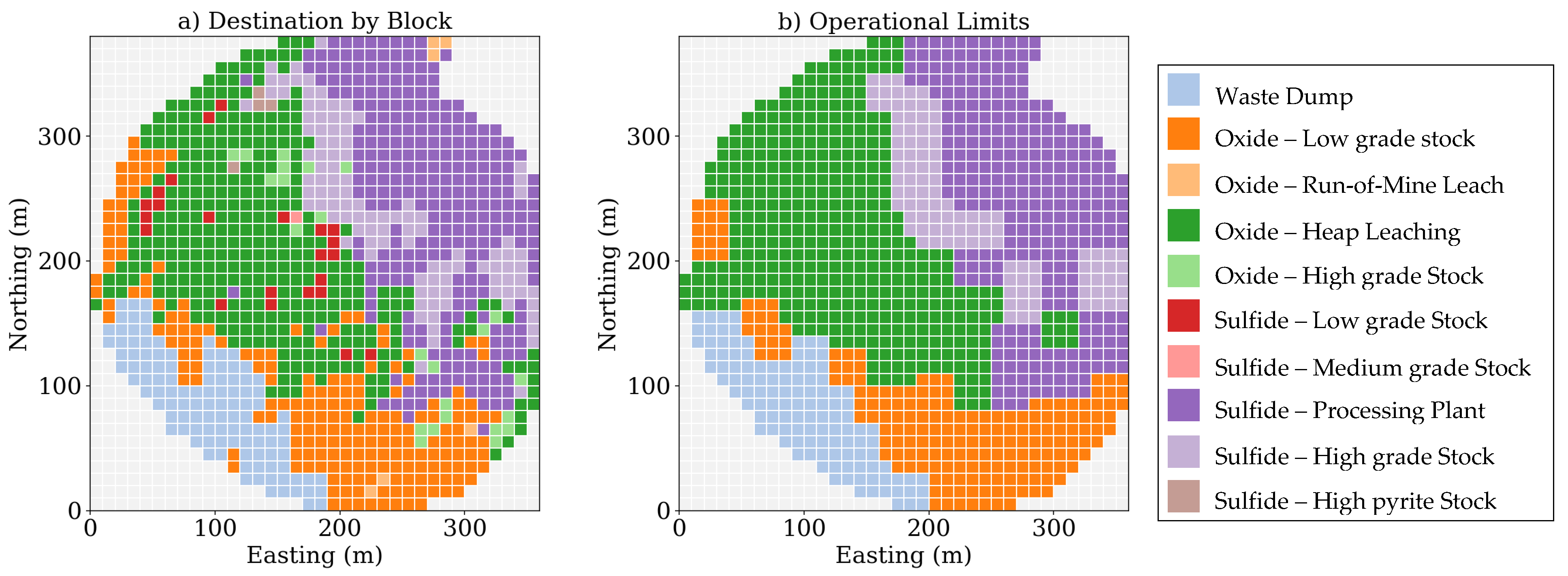
Figure 1 shows an example of the dig-limit definition. In Figure 1a, each block is assigned to its optimal destination based on geological characteristics such as metal content, contaminants, and secondary elements, along with the criteria associated with each processing stream. Figure 1b presents an operational dig-limit configuration, where each block must satisfy an equipment-based operational requirement. Here, a minimum continuous area of 30 × 30 m² was imposed, i.e., each block must have a neighborhood of at least 30 × 30 m² in which all blocks share the same destination. To meet this requirement, geologists adjust the original block-by-block destination assignments, resulting in the modification of the destination of several blocks. These misclassifications reduce the overall profitability of the operation and contribute to misalignment between short- and long-term planning objectives [10,31,32].

Several optimization models and algorithms have been proposed to define optimal dig-limits that maximize profit or enhance compliance with long-term plans. Early research focused on the concept of generating mining polygons, in which a set of vertices is positioned on each bench to delineate ore and waste zones. The dimensions of these polygons and the angles at their vertices were constrained to ensure operational compatibility while simultaneously seeking to maximize the economic value of the resulting assignments. To determine the final positions of the vertices, simulated annealing heuristics were employed, guided by a two-part objective function that sought to maximize economic profit and minimize penalties associated with non-operational or irregular shapes [33,34,35].

Over the past two decades, research has increasingly focused on defining dig-limits at the block level, i.e., determining a destination assignment for each individual block while enforcing an operational metric that reflects equipment selectivity. The minimum operational space has been formalized as a minimum number of contiguous blocks that must share the same destination, a requirement interpreted either as a linear mining width [31] or as a minimum operational shape [9,36]. Various heuristic methods have been proposed to generate or refine solutions under this framework, including greedy algorithms [31], genetic algorithms [9,37,38], random search procedures [39], and simulated annealing [36,40,41]. While these methods satisfy the minimum operational space requirements and consistently produce positive economic outcomes, their reliance on heuristics prevents the guarantee of globally optimal solutions.

More recently, Mixed Integer Programming (MIP) formulations have been introduced to address the dig-limit definition problem. These approaches are typically based on a set-covering framework [42,43], in which each block must be “covered” by at least one feasible operational shape whose constituent blocks share the same destination. This framework has proven both effective in modeling equipment selectivity and tractable when solved using commercial optimization software. Initial studies considered only two destinations and reported revenue improvements of up to 6% compared with manual designs [10,44]. Later works extended this framework to support multiple destinations, reflecting the broader range of routing alternatives present in short-term planning [45]. More recent works incorporate capacity and blending constraints to better represent the requirements associated with each destination [11], with reported gains in profit of up to 7% relative to manual designs.

Notably absent from the dig-limit literature is the explicit incorporation of uncertainty. A major source of uncertainty in this context is grade variability, which can substantially influence ore recovery, processing performance, and overall project profitability. Traditional deterministic planning approaches often fail to capture the stochastic nature of ore deposits, potentially leading to suboptimal or overly risky decisions. In contrast, optimization techniques that explicitly account for uncertainty have proven to be effective in long-term planning, where they enable the development of more robust schedules that better satisfy production targets while improving the expected economic return of the project.

In short-term horizons, even with an increase in geological information from blasthole sampling, grade uncertainty still poses a significant challenge and can impact the compliance with production goals [46,47]. Blasthole data can be unreliable because the sampling process is not always accurate or representative of the true grade of the deposit [48]. In addition, blasthole drilling patterns are often irregular or incomplete, leaving portions of the bench under-sampled and therefore prone to higher estimation error [32,49]. To address short-term uncertainty, geostatistical simulation has become the preferred approach in the mining literature. In this framework, blasthole data serve as an additional source of conditioning information, and multiple grade scenarios are generated through simulation algorithms [48,50,51]. These simulated realizations represent the range of plausible outcomes of the true grade distribution: although each scenario differs from the others, all are consistent with the available sampling data and with the spatial correlation structure of the regionalized variable [52,53,54].

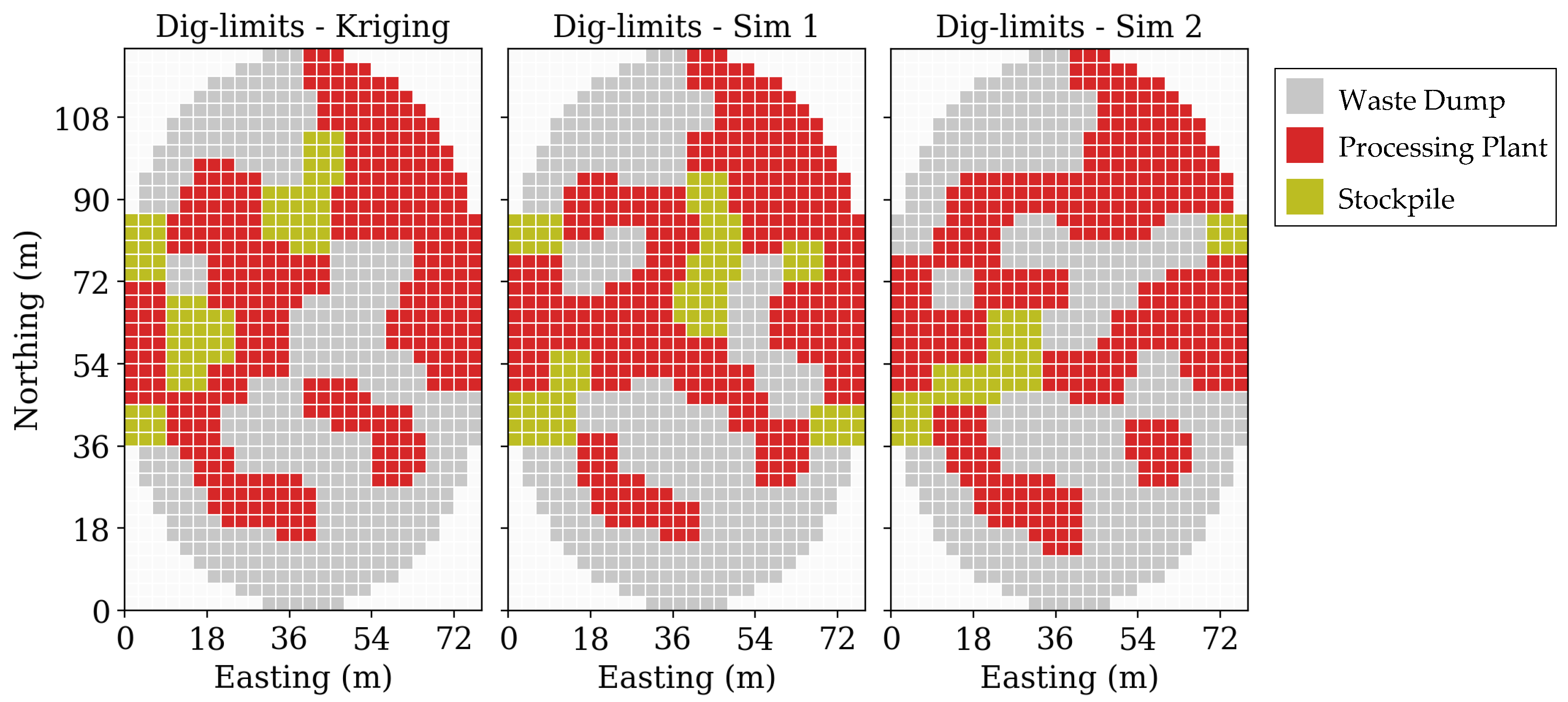
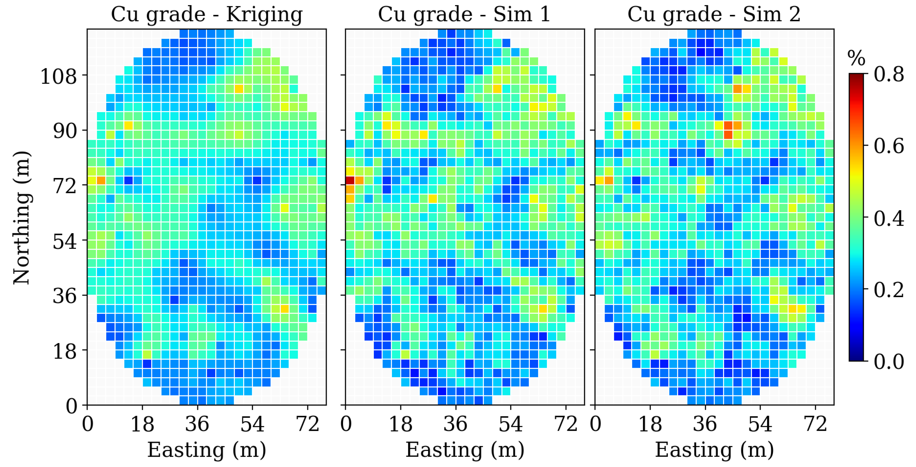
To illustrate the impact of geological variability on the dig-limit definition problem, Figure 2 presents three simulated grade scenarios for a single bench together with their corresponding dig-limit designs. Even when short-term information is available, the resulting dig-limits differ markedly across simulations and relative to the kriged estimate. This variability implies that grade uncertainty can induce misclassification of blocks, ultimately reducing profitability, metal recovery, and compliance with production targets.

Several methods have been proposed to incorporate grade uncertainty into long-term planning models [7,18,55,56,57,58,59]. In contrast, stochastic short-term models, particularly incorporating operational space requirements, remain relatively scarce.

One of the earliest and most widely used approaches in the short-term context is the minimization of deviations from production targets, analogous to long-term stochastic planning models. In these formulations, extraction and destination decisions are selected to maximize an economic objective while simultaneously minimizing deviations from production targets across a set of grade scenarios. Within this framework, several studies have integrated blasthole data to update simulated scenarios or to adjust long-term schedules, thereby reducing short-term variability in production outcomes [50]. The same approach has also been combined with uncertainty in equipment performance, producing short-term plans that better account for both geological and operational variability in single-pit and multi-pit settings when compared with traditional deterministic methods [30,60,61].

Adaptive policies have also been explored for optimizing short-term plans under uncertainty. In this approach, an initial schedule is revised as new information becomes available, typically through additional blasthole samples from recently mined blocks or through updated performance indicators for mining and processing equipment. Early comparisons between a state-dependent adaptive policy and a greedy (max-value) heuristic demonstrated that the adaptive approach yields higher total profit while maintaining ore feed requirements at the processing plant [62]. Rolling-horizon adaptive policies, in which sequential extraction decisions progressively reduce grade uncertainty, have also shown promising results, particularly in settings where geological information is sparse, improving both compliance with production targets and overall profitability [63,64].

Several machine learning techniques have also been proposed within adaptive frameworks, both to approximate the value of new information and to enhance decision-making as the model learns different extraction and destination strategies. Ensemble Kalman filters have been applied to update geological information using blasthole samples [29,65], while deep neural networks have been employed to estimate the value and performance of short-term extraction and destination decisions [66]. Reinforcement learning frameworks have shown promising results in learning and updating short-term policies and equipment allocation decisions to improve compliance with long-term production goals and short-term cash-flow when compared with fixed schedules that do not incorporate updating mechanisms [29,65,66,67,68,69].

While previous research provides several approaches for managing uncertainty in short-term horizons, the consideration of loading-equipment selectivity remains largely absent. Most studies assume that short-term decisions can be made independently for each block. However, in practice, operational cuts or dig-limits must be defined to reflect the actual digging dynamics and selectivity constraints of shovel equipment [52].

In the mining-cut literature, where distinct volumes are defined for daily or weekly extraction, the incorporation of uncertainty has been limited and predominantly addressed through heuristic approaches. Hierarchical clustering based on possible worlds [70] and loss functions [52] has been used to generate mining cuts that account for uncertainty in grade distribution [29,71]. These methods rely on distance metrics that summarize information across multiple grade simulations to guide cluster formation.

The first application of a stochastic Mixed Integer Program for generating mining cuts was developed under the framework of minimizing deviations from production targets [72]. This model extended a previous deterministic formulation that enforced destination-based precedence constraints between blocks to satisfy minimum operational space requirements in short-term production schedules [28]. Although this stochastic model achieved improvements in economic value and target compliance compared with its deterministic counterpart [28], it was unable to guarantee the operational compatibility of the resulting mining cuts in all cases.

For the dig-limit definition problem, risk-minimization approaches have been proposed to incorporate geological uncertainty. In these formulations, a moving-neighborhood heuristic aggregates blocks based on their expected value while simultaneously attempting to minimize a risk measure evaluated over a set of simulated grade scenarios [73]. More recent studies have introduced a multi-step methodology to account for grade uncertainty arising from both geological variability and blasthole movement [44,45]. In this approach, simulated scenarios are generated by combining grade realizations conditioned on blasthole data with movement simulations derived from blasting-tracker measurements. These scenarios are then pre-processed to determine an optimal destination for each block based on the maximum expected profit across all simulations. The resulting destinations are subsequently incorporated into a deterministic dig-limit optimization model to obtain a final set of operationally compatible destinations.

To the best of our knowledge, there are currently no stochastic formulations for the dig-limit definition problem that can be solved to optimality. Such formulations would be highly valuable for designing destination policies that perform well across a wide range of geological scenarios, maximizing expected value while controlling the risk of failing to meet production goals, particularly in situations where blasthole sampling is incomplete or imperfect.

In this work, we propose a stochastic formulation of the dig-limit definition problem based on the minimization-of-deviations framework. The main contribution of this study is the development of an efficient optimization model that delivers dig-limit definitions that maximize the expected profit of destination assignments, satisfy operational selectivity constraints, and minimize deviations from both short- and long-term production targets under grade uncertainty. In contrast to previous approaches, this is, to the best of our knowledge, the first optimization model to explicitly incorporate grade scenarios within the mathematical formulation to control production deviations, while remaining solvable to optimality using a general-purpose solver.

2. Materials and Methods

In this section, we present the methodological approach developed to incorporate grade uncertainty into the dig-limit definition problem. We begin by outlining the general framework and the key assumptions adopted to emulate the decision-making process used in short-term planning under geological uncertainty. Then, we introduce the mathematical formulation of the Stochastic Dig-Limit Optimization Program (ST-DIGOPT), which formalizes the integration of multiple grade realizations into a unified optimization model.

2.1. Framework for Short-Term Dig-Limit Definition Under Uncertainty

As discussed in the literature review, several studies have proposed optimization frameworks that explicitly incorporate geological uncertainty into mine planning models. A common assumption in these approaches is that uncertainty can be quantified and represented through a collection of equiprobable scenarios, each honoring the available hard data and reflecting the expected variability in the underlying uncertain variables. In line with this perspective, our work assumes that it is possible to generate multiple grade scenarios that honor the most recent and operationally relevant information: blasthole samples. These samples constitute the final source of geological data acquired immediately before extraction and destination decisions are executed.

In most stochastic mine planning models, uncertainty in the input parameters is addressed through a two-stage modeling approach, in which first-stage variables are fixed across all scenarios, and new information triggers a second-stage decision that may vary by scenario and correct any inaccurate assumptions made initially. For example, in long-term stochastic models under grade uncertainty, first-stage decisions typically correspond to the extraction sequence, defined using drillhole data and enforced to maximize NPV. In the short-term, these models commonly assume a recourse action in the form of destination decisions. Once blasthole data becomes available, the updated geological information allows the model to distinguish between scenarios and assign different destinations to each block, ensuring compliance with processing, blending, or other operational constraints while maximizing NPV in each scenario, subject to the first-stage mining sequence.

In short-term horizons, however, the relevant source of uncertainty is post–blasthole information, that is, the imperfection of the blasthole sampling strategy. Because we consider uncertainty after the “true” grade of the bench is revealed, we cannot rely on the same decision framework used in long-term models. For this reason, we follow the approach described in previous short-term stochastic models [72]. Since no additional information becomes available after the blasthole data that could justify adjusting destinations, we treat the destination policy defined by the dig-limits as a first-stage decision that must remain fixed across all scenarios. The only recourse action in this context is the management of deviations from production targets in each scenario. Each geological simulation produces a different grade distribution, and therefore the fixed destination policy yields scenario-specific metal production and grade outcomes. To ensure compliance with long-term production goals, our stochastic dig-limit formulation seeks to minimize the deviations of these quantities from their respective targets in each scenario, as described in the following section.

2.2. Mathematical Formulation

In this section, we present the optimization model used to incorporate geological uncertainty into the dig-limit definition problem. The formulation extends a previous deterministic model for dig-limit definition with multiple destinations, originally described in [11].

Formally, let $\mathcal{B}$ be the set of blocks in a bench and $\mathcal{D}$ the set of available destinations in the mining operation. The true grade of each block $b\in \mathcal{B}$ is unknown but can be described through a set of geological scenarios $\mathcal{S}$. Each block must be assigned to one destination, and this assignment yields a profit that depends on the destination specifications, block attributes, and the geological scenario, denoted as $p_{bds}$. Equivalently, in the case where uncertainty is not considered, the expected profit for each block–destination pair is denoted as ${\widehat{p}}_{vd}$, computed from the estimated block attributes.

The destination assignment must satisfy the operational requirements imposed by shovel selectivity. We assume a minimum operational requirement represented by a structuring element, whose size and shape are determined by the loading equipment assigned to each destination. Let ${\mathcal{F}}_d$ be the set of structuring elements that satisfy the selectivity requirements for $d\in \mathcal{D}$. Each structuring element $f\in {\mathcal{F}}_d$ covers a subset of blocks denoted as ${\mathcal{B}}_f\subset \mathcal{B}$, defined as those located within its spatial limits. The size of set ${\mathcal{B}}_f$ is denoted by $k_f$, which represent the number of blocks covered by element $f$. If all blocks $b\in {\mathcal{B}}_f$ are assigned to the same destination, the structuring element $f$ generates a valid cover. This valid-cover condition ensures that the destination assignment is compatible with the loading equipment selectivity. To produce a feasible dig-limit definition, every block $b$ must belong to at least one subset ${\mathcal{B}}_f$ for which $f$ generates a valid cover. Because different structuring elements may cover the same block, we define ${\mathcal{F}}_d^b$ as the set of structuring elements compatible with the selectivity requirements of destination $d$ that cover block $b$.

The assignment is also constrained by resources requirements at each destination. Destinations may impose hard limits on the utilization of certain resources. For example, a processing plant may specify a maximum allowable tonnage or require a minimum throughput for operational stability. Let $\mathcal{R}$ be the set of resources associated with the destination assignment. When a block $b$ is assigned to a destination $d$, it consumes an amount $w_{rbd}$ of resource $r\in \mathcal{R}$. Each resource has upper and lower bounds, ${\overline{W}}_{rd}$ and ${\underset{¯}{W}}_{rd}$, respectively, and a feasible destination assignment must satisfy both.

Additional constraints may arise from average-grade requirements at the destinations. A plant may impose upper and lower limits on the average content of metals or contaminants to avoid processing inefficiencies, and stockpiles may be defined by grade ranges to maintain controlled metal content for future periods. Let $\mathcal{Q}$ be the set of relevant grades attributes. Each block $b$ has a grade $g_{qbd}$ associated with its assignment to a destination $d$. The average grade of element $q\in \mathcal{Q}$ of all blocks assigned to destination $d$ must lie within the bounds ${\overline{G}}_{qd}$ and ${\underset{¯}{G}}_{qd}$. Note that for the average grade calculation, a weight parameter is also defined, which usually comes from the set of resources and is also denoted as $w_{rbd}$.

To introduce grade variability, we incorporate desired (soft) production targets. These targets represent the preferred production outcomes for each destination but are not enforced as hard constraints. Instead, deviations from the targets across scenarios are penalized in the objective function. We define production targets ${\widehat{W}}_{rd}$, representing the desired utilization of resource $r$ at destination $d$, and average-grade targets ${\widehat{G}}_{qd}$, representing the desired mean grade of element $q$ of all blocks assigned to destination $d$. Deviations from these targets are penalized using cost parameters, ${\overline{c}}_{rd}$ and ${\underset{¯}{c}}_{rd}$ for resource targets, and ${\overline{c}}_{qd}$ and ${\underset{¯}{c}}_{qd}$ for grade targets. These costs reflect the expected economic loss associated with failing to meet the targets, although they may also serve as tuning parameters to control the strictness of target compliance.

To evaluate deviations under uncertainty, we denote by $w_{rbds}$ the amount of resource $r$ consumed when block $b$ is assigned to destination $d$ in scenario $s$, and by $g_{qbds}$ the corresponding grade of element $q$ in block $b$ when assigned to destination $d$ in scenario $s$. Decision variables are defined in Equations (1)–(6).

$$x_{bd}=\left\{\begin{array}{c}1, \mathrm{i}\mathrm{f} \mathrm{b}\mathrm{l}\mathrm{o}\mathrm{c}\mathrm{k} b \mathrm{i}\mathrm{s} \mathrm{a}\mathrm{s}\mathrm{s}\mathrm{i}\mathrm{g}\mathrm{n}\mathrm{e}\mathrm{d} \mathrm{t}\mathrm{o} \mathrm{d}\mathrm{e}\mathrm{s}\mathrm{t}\mathrm{i}\mathrm{n}\mathrm{a}\mathrm{t}\mathrm{i}\mathrm{o}\mathrm{n} d \\ 0, \mathrm{o}\mathrm{t}\mathrm{h}\mathrm{e}\mathrm{r}\mathrm{w}\mathrm{i}\mathrm{s}\mathrm{e} \end{array}\right.$$

(1)

$$v_{fd}=\left\{\begin{array}{c}1, \mathrm{i}\mathrm{f} \mathrm{a}\mathrm{l}\mathrm{l} \mathrm{b}\mathrm{l}\mathrm{o}\mathrm{c}\mathrm{k}\mathrm{s} b\in {\mathcal{B}}_f are \mathrm{a}\mathrm{s}\mathrm{s}\mathrm{i}\mathrm{g}\mathrm{n}\mathrm{e}\mathrm{d} \mathrm{t}\mathrm{o} \mathrm{d}\mathrm{e}\mathrm{s}\mathrm{t}\mathrm{i}\mathrm{n}\mathrm{a}\mathrm{t}\mathrm{i}\mathrm{o}\mathrm{n} d \in D \\ 0, \mathrm{o}\mathrm{t}\mathrm{h}\mathrm{e}\mathrm{r}\mathrm{w}\mathrm{i}\mathrm{s}\mathrm{e} \end{array}\right.$$

(2)

$${\overline{e}}_{rds}=\mathrm{Surplus} \mathrm{from} \mathrm{production} \mathrm{target} {\widehat{W}}_{rd}\mathrm{in} \mathrm{scenario} s\in \mathcal{S}$$

(3)

$${\underset{¯}{e}}_{rds}=\mathrm{Deficit} \mathrm{from} \mathrm{production} \mathrm{target} {\widehat{W}}_{rd}\mathrm{in} \mathrm{scenario} s\in \mathcal{S}$$

(4)

$${\overline{e}}_{qds}=\mathrm{Surplus} \mathrm{from} \mathrm{average} \mathrm{target} \mathrm{grade} {\widehat{G}}_{qd}\mathrm{in} \mathrm{scenario} s\in \mathcal{S}$$

(5)

$${\underset{¯}{e}}_{qds}=\mathrm{Deficit} \mathrm{from} \mathrm{average} \mathrm{target} \mathrm{grade} {\widehat{G}}_{qd}\mathrm{in} \mathrm{scenario} s\in \mathcal{S}$$

(6)

The optimization model for the Stochastic Dig-limit Problem (hereafter referred to as (ST-DIGOPT)) is presented through Equations (7)–(21). Appendix B offers a summary of all parameters, variables and sets used in the formulation.

$$\max {\displaystyle \frac{1}{\left|S\right|}}\sum _{s\in \mathcal{S}}\sum _{d\in \mathcal{D}}\left(\sum _{b\in \mathcal{B}}{p}_{bds}{x}_{bd}-\sum _{q\in \mathcal{Q}}\left({\overline{e}}_{qds}{\overline{c}}_{qd}+{\underset{¯}{e}}_{qds}{\underset{¯}{c}}_{qd}\right)-\sum _{r\in \mathcal{R}}({\overline{e}}_{rds}{\overline{c}}_{rd}+{\underset{¯}{e}}_{rds}{\underset{\_}{c}}_{rd})\right)$$

(7)

$$s.t. v_{fd}\le {\displaystyle \frac{1}{k_f}}\sum _{b\in {\mathcal{B}}_f}{x}_{bd} \forall d\in \mathcal{D},f\in {\mathcal{F}}_d$$

(8)

$$\sum _{d\in D}\sum _{f\in {\mathcal{F}}_d^b}{v}_{fd}\ge 1 \forall b\in \mathcal{B}$$

(9)

$$\sum _{d\in \mathcal{D}}{x}_{bd}=1 \forall b\in \mathcal{B}$$

(10)

$$\sum _{b\in \mathcal{B}}{x}_{bd}{w}_{rbd}\ge {\underset{¯}{W}}_{rd} \forall d\in \mathcal{D},r\in \mathcal{R}$$

(11)

$$\sum _{b\in \mathcal{B}}{x}_{bd}{w}_{rbd}\le {\overline{W}}_{rd} \forall d\in \mathcal{D},r\in \mathcal{R}$$

(12)

$$\sum _{b\in \mathcal{B}}\left({\overline{G}}_{qd}-g_{qb}\right)x_{bd}{w}_{rbd}\ge 0 \forall d\in \mathcal{D},r\in \mathcal{R},q\in \mathcal{Q}$$

(13)

$$\sum _{b\in \mathcal{B}}\left({\underset{¯}{G}}_{qd}-g_{qb}\right)x_{bd}{w}_{rbd}\le 0 \forall d\in \mathcal{D},r\in \mathcal{R},q\in \mathcal{Q}$$

(14)

$$\sum _{b\in \mathcal{B}}{x}_{bd}{w}_{rbds}+{\underset{¯}{e}}_{rds}\ge {\widehat{W}}_{rd} \forall d\in \mathcal{D},r\in \mathcal{R},s\in \mathcal{S}$$

(15)

$$\sum _{b\in \mathcal{B}}{x}_{bd}{w}_{rbds}-{\overline{e}}_{rds}\le {\widehat{W}}_{rd} \forall d\in \mathcal{D},r\in \mathcal{R},s\in \mathcal{S}$$

(16)

$$\sum _{b\in \mathcal{B}}\left({\widehat{G}}_{qd}-g_{qbs}\right)x_{bd}{w}_{rbds}+{\underset{¯}{e}}_{qds}\ge 0 \forall d\in \mathcal{D},r\in \mathcal{R},q\in \mathcal{Q},s\in \mathcal{S}$$

(17)

$$\sum _{b\in \mathcal{B}}\left({\widehat{G}}_{qd}-g_{qbs}\right)x_{bd}{w}_{rbds}-{\overline{e}}_{qds}\le 0 \forall d\in \mathcal{D},r\in \mathcal{R},q\in \mathcal{Q},s\in \mathcal{S}$$

(18)

$$v_{fd}\in \left\{\mathrm{0,1}\right\} \forall f\in {\mathcal{F}}_d,d\in \mathcal{D}$$

(19)

$$x_{bd}\in \left\{\mathrm{0,1}\right\} \forall b\in \mathcal{B},d\in \mathcal{D}$$

(20)

$${\underset{¯}{e}}_{qds}, {\overline{e}}_{qds}\in {\mathbb{R}}_0^{+} \forall q\in \mathcal{Q},d\in \mathcal{D},s\in \mathcal{S}$$

(21)

$${\underset{¯}{e}}_{rds}, {\overline{e}}_{rds}\in {\mathbb{R}}_0^{+} \forall r\in \mathcal{R},d\in \mathcal{D},s\in \mathcal{S}$$

(22)

Equation (7) defines the objective function, which comprises three components: the profit from the destination assignment, the deviation costs associated with resource production targets, and the deviation costs associated with average grade targets. All three components are averaged over the set of geological scenarios in a risk-neutral manner.

Equation (8) imposes the valid-cover constraint. For each structuring element, the right-hand side counts how many blocks are assigned to a given destination. If this count matches the size of the structuring element, $k_f$, the expression evaluates to 1, indicating that all blocks within the structuring element share the same destination, and therefore the cover is valid. In such cases, variable $v_{fd}$ is allowed to take the value 1. This constraint enforces the minimum selectivity requirement for each destination, since the size and shape of the structuring elements are fully determined by the shovel equipment used in the operation. Equation (8) operates jointly with Equation (9), which requires every block in the bench to be covered by at least one valid structuring element. Together, these constraints ensure that any feasible solution to (ST-DIGOPT) satisfies the operational requirements of the dig-limit definition problem.

Equation (10) ensures that every block is assigned to exactly one destination. Note that leaving a block unextracted is not an option within this planning horizon, as all material in short-term plans must be mined to comply with the long-term extraction sequence.

Equations (11) and (12) impose the resource-limit constraints. For each destination and each resource considered in the planning horizon, the total amount of resource contributed by all blocks assigned to the destination must fall within the specified bounds. This constraint is general, and in some cases no practical limit exists for a given resource–destination pair. For instance, waste dumps are typically modeled as destinations with no tonnage restriction. For this case, the lower bound, ${\underset{¯}{W}}_{rd}$, can be set to zero and the upper bound ${\overline{W}}_{rd}$ to infinity. For simplicity, we refer explicitly to resource constraints only when the corresponding upper bound is finite or the lower bound is nonzero.

Equations (13) and (14) represent the average grade constraints of the destination assignment. The average grade of all blocks sent to a given destination must satisfy the corresponding quality requirements in terms of metal grades and contaminants. As with the resource constraints, and for simplicity, we explicitly refer to average grade constraints only for those triples ($d,r,q)\in \mathcal{D}\times \mathcal{R}\times \mathcal{Q}$ for which the upper limit ${\overline{G}}_{qd}$ is finite or the lower limit ${\underset{¯}{G}}_{qd}$ is nonzero.

Equations (15) and (16) quantify the deviations from the production targets. These constraints resemble the resource limit constraints but incorporate deviation variables. These variables record the shortfall or excess with respect to the production target in each scenario, given that the destination assignment is fixed across all scenarios as a first-stage decision. For instance, if the total production of resource $r$ assigned to destination $d$ in scenario $s$ is lower than the target ${\widehat{W}}_{rd}$, the corresponding deviation variable ${\underset{¯}{e}}_{rds}$ in Equation (15) captures this deficit to satisfy the constraint. Although the deviation variable could take any value greater than ${\widehat{W}}_{rd}-\sum _{b\in \mathcal{B}}{x}_{bd}{w}_{rbds}$ to maintain feasibility, the objective function penalizes deviations, ensuring that the model sets each deviation variable exactly equal to the actual shortfall or excess relative to the target.

Equations (17) and (18) define the analogous deviation constraints for average grade targets. These constraints function similarly to Equations (13) and (14) but include additional variables that measure the deviation from the desired average grade in each scenario.

Finally, Equations (19)–(22) specify the domain of all decision variables.

2.3. Experimental Setup

To evaluate the performance of the proposed optimization model, we consider two case studies based on real data from copper deposits located in northern and central Chile. For both cases, we showcase different applications of (ST-DIGOPT).

In the first case, we apply (ST-DIGOPT) to control deviations from total metal production targets, ensuring steady metal output across the set of grade scenarios. In the second case, deviations are used to regulate the average grade of the material sent to the processing plant, thereby promoting optimal performance in the recovery stage. A detailed description of each case study is provided in Section 3.

To compare the value of applying the proposed stochastic formulation, we report four types of dig-limit definitions for both case studies:

(1)

Stochastic Definition: These dig-limits are obtained by applying (ST-DIGOPT) to each case study. In both cases, we use 20 grade scenarios as the set of simulations.

(2)

Deterministic Definition: These limits are obtained by applying the deterministic variant of ST-DIGOPT, which is equivalent to using a single estimated scenario as the complete set of simulations. For both case studies, we use an ordinary kriging grade estimate as the deterministic scenario.

(3)

Manual Definition: These limits are generated manually by a mining engineer with prior experience in defining dig-limits in copper deposits. The engineer was provided with the kriged grade distribution, the cut-off grade, the minimum selectivity size imposed by the loading equipment, and the desired production targets. The dig-limits were defined by prioritizing profit maximization, while attempting to meet the production targets as a secondary objective. The resulting dig-limit definition was required to satisfy the hard constraints of the problem, namely the minimum selectivity size and resource bounds. Although no strict time limit was imposed, the engineer completed the task in approximately 30 min for each case study.

(4)

Perfect Knowledge Definitions: In this case, we obtain a distinct dig-limit definition for each simulated grade scenario by applying the deterministic variant of (ST-DIGOPT). This corresponds to assuming perfect knowledge of the deposit before defining dig-limits. Such information is unattainable in practice, so this solution provides a clairvoyant upper bound on the maximum achievable profit in each scenario and serves as a benchmark for other definitions.

To evaluate the performance of (ST-DIGOPT), we use different simulation sets. As noted earlier, a training set of 20 scenarios is employed to obtain the stochastic definition. A separate set of 100 scenarios is used as the testing set. These scenarios, although not used in the construction of the stochastic dig-limit definition, are representative of the expected variability of the deposit. All results presented in Section 3 were evaluated using the testing set, while the results obtained for the training set are provided in Appendix A. To assess whether the differences in profit between definitions were statistically significant, we applied a paired t-test on the average profit across grade scenarios, using a p-value threshold of 0.05.

Finally, we analyze the impact of the number of scenarios used in the training set for (ST-DIGOPT). For both case studies, we vary the size of the training set and evaluate the resulting dig-limit definition over an independent testing set to assess how the number of grade simulations affects profit and production deviations. In addition, we provide a brief analysis of the impact of the training set size on the computational performance of the proposed model. All cases were implemented in Python 3.12 and solved using Gurobi 12.0.1 on a laptop equipped with an Intel Core i7-1365U processor (Intel Corporation, Santa Clara, CA, USA) and 16 GB of RAM.

2.4. Cases Description

2.4.1. Case A

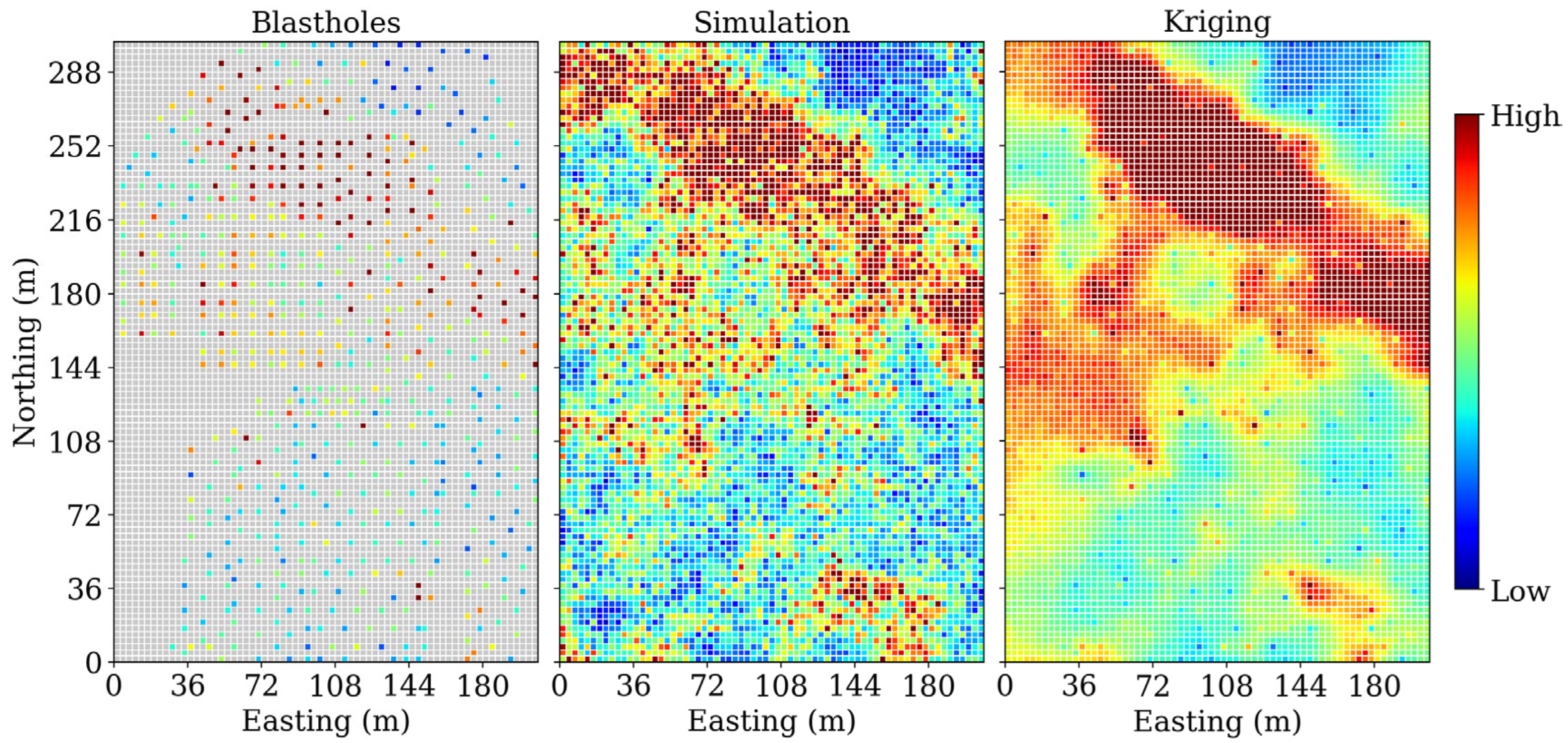
This case study corresponds to a porphyry copper deposit located in northern Chile. We extracted a single bench section from a former production phase. The blasthole pattern is regular but incomplete: some areas of the bench were not sampled during mining operations. This gap in sampling is attributable to the low geological variability expected in that zone. The bench comprises 6969 blocks (set of blocks, $\mathcal{B}$) and 656 blastholes. The average copper grade of the blastholes is 0.46%, with a standard deviation of 0.21%. For this case study, the set of simulations, $\mathcal{S}$, includes 120 grade realizations generated by the mining operation from blasthole data using the Sequential Gaussian Simulation algorithm [74]. A kriging grade estimate was also provided by the company. The minimum selectivity size is defined as 3 × 3 blocks (9 × 9 m²). Figure 3 presents the blasthole data, the kriging estimate, and a representative simulation for this case study.

The bench is scheduled to be extracted within a single month, which imposes a strict upper limit on the processing capacity of 1.4 Mt of ore. The remaining material can either be stockpiled for later processing or discarded if its metal content falls below the cut-off grade. Accordingly, three possible destinations were considered in the model ($\mathcal{D}$): processing plant, stockpile and waste dump. To enforce the maximum plant capacity, Equation (12) was applied using $w_{rbd}$ as the tonnage ($r$) of the block ($b$) processed in the plant ($d$) and ${\overline{W}}_{rd}$ set to 1.4 Mt. For this case study, a steady metal production of 7000 t is targeted. Thus, an additive deviation constraint was included following Equation (15) and (16), with the metal content ($r$) of the block ($b$) in each simulation ($s$) assigned to the processing plant ($d$) defined as the additive attribute $w_{rbds}$, and a production target ${\widehat{W}}_{rd}$ of 7000 t. Note that the metal content varies across simulations because it depends on the block’s grade.

The use of an additive deviation constraint requires specifying deviation costs ${\underset{\_}{c}}_{rd}$ and ${\overline{c}}_{rd}$. For this case, both the underproduction and overproduction penalties were set to 1000 USD/t to promote a stable production profile. The profit associated with each block and destination, $p_{bds}$, was calculated using Equation (23), with the economic parameters summarized in

Table 1. Economic Parameters.

Parameter	Waste Dump	Plant	Stockpile
Mine Cost ($Mcost$) (USD/t)	1.8	1.8	1.8
Processing Cost ($Pcos{t}_d$) (USD/t)	0	12	13.5
Recovery ($Re{c}_d$)	0	0.88	0.88
Refinement Cost ($Rcos{t}_d$) (USD/lb Cu)	0	0.4	0.4
Copper Price ($C{u}_{price}$) (USD/lb Cu)	3.5	3.5	3.5
Discount rate ($dis{c}_d$)	0	0	0.01

. It is important to note that the stockpile option involves higher processing costs to account for material reclamation, as well as a small discount rate reflecting the deferred revenue associated with processing the material in future periods.

$$p_{bds}={\displaystyle \frac{w_{tonnage,bd}}{(1+dis{c}_d)}}\left(\left(C{u}_{price}-Rcos{t}_d\right)Re{c}_d\times g_{cu,bs}\times 2204.6-\left(Mcost+Pcos{t}_d\right)\right)$$

(23)

2.4.2. Case B

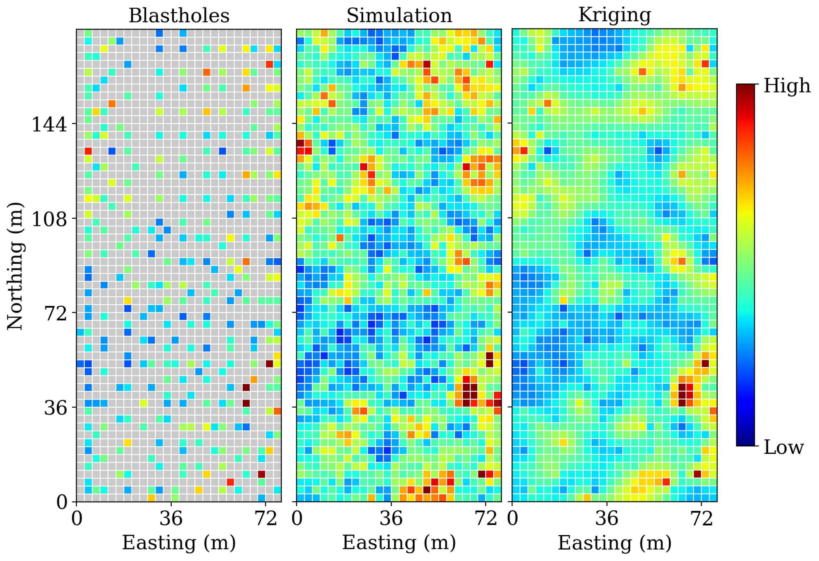
Case B corresponds to a low-grade copper deposit located in central Chile. The mining company provided a medium-sized bench with 1560 blocks ($\mathcal{B}$). The blasthole dataset contains 327 samples arranged in a pseudo-regular pattern. The average blasthole grade is 0.36%, with a standard deviation of 0.12%. Based on these data, 120 grade scenarios were obtained, together with an ordinary kriging estimate. Because small shovels are used in this operation, a minimum selectivity size of 2 × 2 blocks (6 × 6 m²) was imposed for all destinations (6 × 6 m²). Figure 4 shows the blasthole data, the estimated scenario and one simulated scenario for this case study.

In this case study, the processing plant has an upper capacity limit of 280,000 t per week, which corresponds to the expected planning horizon for the bench. Consequently, Equation (12) was imposed with $w_{rbd}$ representing the tonnage ($r$) of the block ($b$) sent to the plant ($d$), and ${\overline{W}}_{rd}$ set to 280 kt. The remaining material can either be sent to the waste dump or stored for later processing in the stockpile.

A critical operational constraint is the weekly average grade of the material sent to the processing plant. To ensure proper metallurgical performance, an average grade of 0.45% is required. Because ore grades fluctuate across scenarios, we imposed Equations (17) and (18) to control deviations from this target. Specifically, $g_{qbs}$ was defined as the copper grade ($q$) of the block ($b$) in a simulated scenario $\left(s\right)$, weighted by the block tonnage, $w_{rbd}$, and the target average copper grade in the processing plant, ${\widehat{G}}_{qd}$, was set to 0.45%. Deviation costs were fixed at 25 USD/t.

Block valuation for each destination and simulation was calculated using Equation (23) with the same economic parameters reported in Table 1.

3. Results

In this section, we present the main results obtained using (ST-DIGOPT) for both case studies described previously. We compare the resulting dig-limit definitions, the expected tonnage assigned to each destination, the profit distribution across scenarios, and the deviations from the corresponding production targets.

3.1. Case A

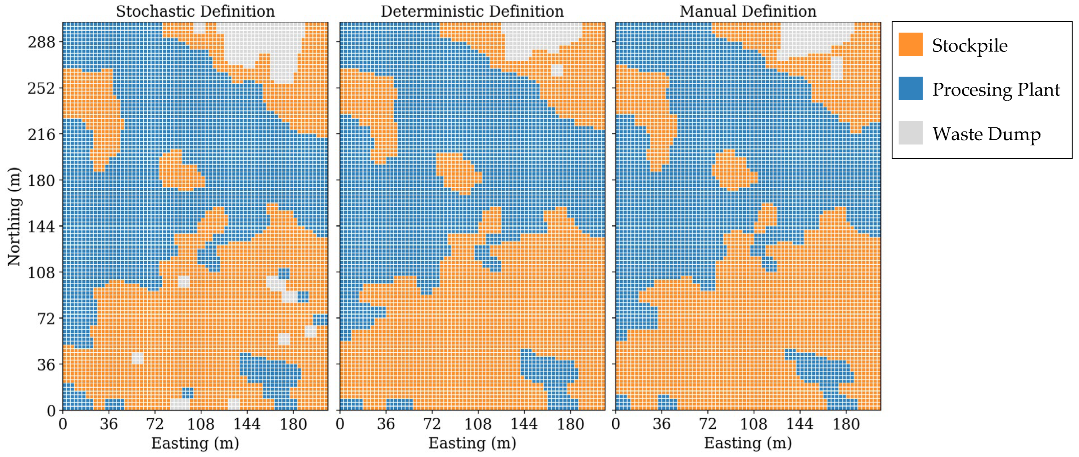
The first set of results corresponds to the dig-limit definitions obtained with the stochastic, deterministic, and manual approaches. Figure 5 presents the three resulting definitions. All solutions fully comply with the minimum selectivity size of 9 × 9 m² imposed for this case study.

As shown in the figure, because most of the bench lies above the cut-off grade, the majority of blocks are classified either as ore for the processing plant or as stockpile material. All definitions tend to saturate the plant’s maximum capacity, sending the remaining ore blocks to the stockpile. While the Deterministic and Manual definitions are quite similar, the Stochastic formulation assigns less material to the stockpile This aligns with the Perfect Knowledge definitions, which, on average, allocate even less material to the stockpile. For this case study, incorporating grade scenarios appears to reduce the number of blocks classified as ore, reflecting the variability observed across simulations. Following the same trend, waste assignment also varies across definitions: the Stochastic model classifies 148.4 kt as waste, whereas the Deterministic and Manual definitions are less conservative, classifying 86.7 kt and 87.9 kt, respectively. Because both the Deterministic and Manual definitions rely on the kriged estimate, they exhibit similar tonnage allocation patterns.

Table 2. Tonnage and Average grade by destination for each definition—Case A.

Definition	Waste Dump		Plant		Stockpile
	Tonnage (kt)	Grade (%)	Tonnage (kt)	Grade (%)	Tonnage (kt)	Grade (%)
Deterministic	86.7	0.192 ± 0.017	1399.5	0.493 ± 0.013	1323.7	0.441 ± 0.011
Stochastic	148.4	0.218 ± 0.012	1393.5	0.532 ± 0.011	1268.1	0.407 ± 0.012
Perfect Knowledge	269.1 ± 73.5	0.206 ± 0.012	1398.4 ± 7.1	0.531 ± 0.003	1142.4 ± 74.4	0.431 ± 0.023
Manual	87.9	0.192 ± 0.016	1389.8	0.48 ± 0.013	1332.2	0.455 ± 0.009

summarizes the tonnages and grades by destination for all definitions.

Although ore tonnage sent to the plant is similar across definitions, the Stochastic formulation yields a higher average grade, making better use of the available plant capacity and increasing metal output. This result is consistent with the expected metal production target imposed in the case study. In contrast, the grade of the material assigned to the stockpile is lower across scenarios compared with both the Manual and Deterministic solutions.

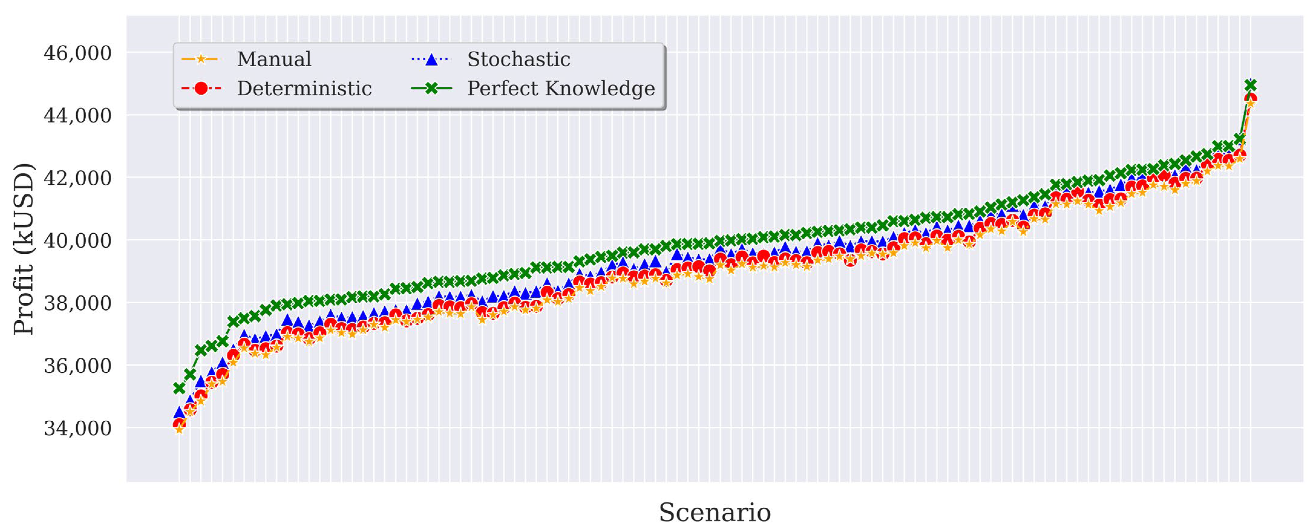
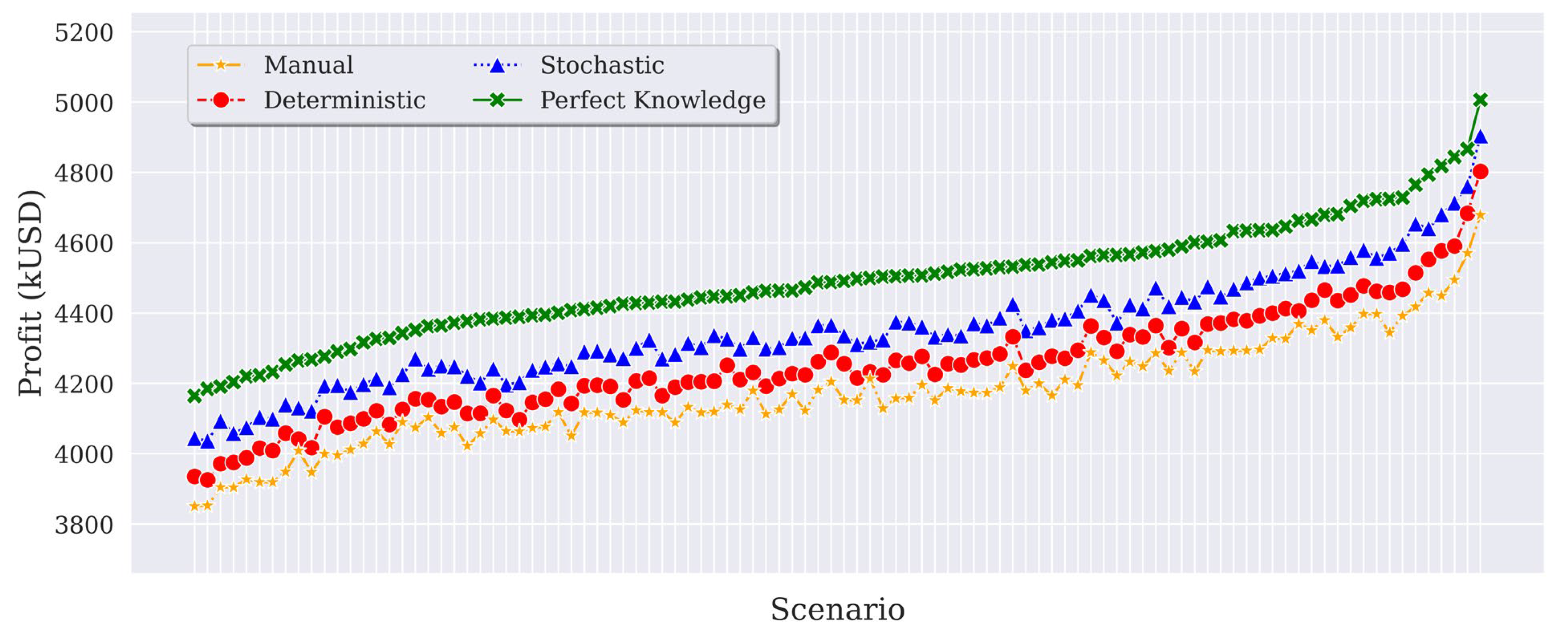
In this case study, a considerable number of blocks shift their classification between the plant and the stockpile across the three definitions. However, both destinations yield similar levels of profit according to Equation (23). Thus, even if the dig-limit maps appear different, these destination changes may not meaningfully affect the total profit. To assess the magnitude of this effect, we evaluated the performance of all definitions over the testing set of 100 scenarios, as shown in Figure 6.

The profit differences among the definitions are relatively small, primarily since the two ore destinations yield similar economic outcomes. Therefore, variations in the dig-limit definitions do not translate into substantial profit differences in this case study, where most of the bench is classified as ore. However, the expected profit shows small but statistically significant differences. The deterministic definition achieves a 0.36% higher profit than the Manual definition (p-value = 3.44 × 10⁻³⁴), while the Stochastic definition outperforms the deterministic one by 0.86% (p-value = 2.55 × 10⁻⁶⁰). Overall, adopting the stochastic definition instead of the manual one results in an average profit increase of 1.22% (p-value = 3.55 × 10⁻⁷²). Finally, the value of information, defined as the expected difference between the Stochastic and Perfect Knowledge definitions, is 1.17% (p-value = 5.46 × 10⁻⁴⁰).

In terms of profit dispersion, all definitions exhibit substantial variability across scenarios. For instance, the interpercentile range between the 95th and 5th percentiles is large for all four definitions, varying from 5.65 MUSD for the perfect knowledge definition to 6.07 MUSD for the deterministic one. These ranges correspond to between 14.1% and 15.4% of the average profit, depending on the definition. This result indicates that even in cases with limited variability in destination assignment, a single dig-limit policy can lead to markedly different economic outcomes across grade scenarios.

Table 3. Average profit and deviation costs by definition—Case A.

Definition	Avg. Profit (kUSD)	Avg. Deviation Cost (kUSD)
Deterministic	39,092.9 ± 1946.5	586.5 ± 187.5
Stochastic	39,428.9 ± 1933.6	131 ± 101.9
Perfect Knowledge	39,890.1 ± 1756.1	3.7 ± 11.3
Manual	38,953.1 ± 1960.9	818.6 ± 198.3

provides a summary of profit and deviation costs for each definition.

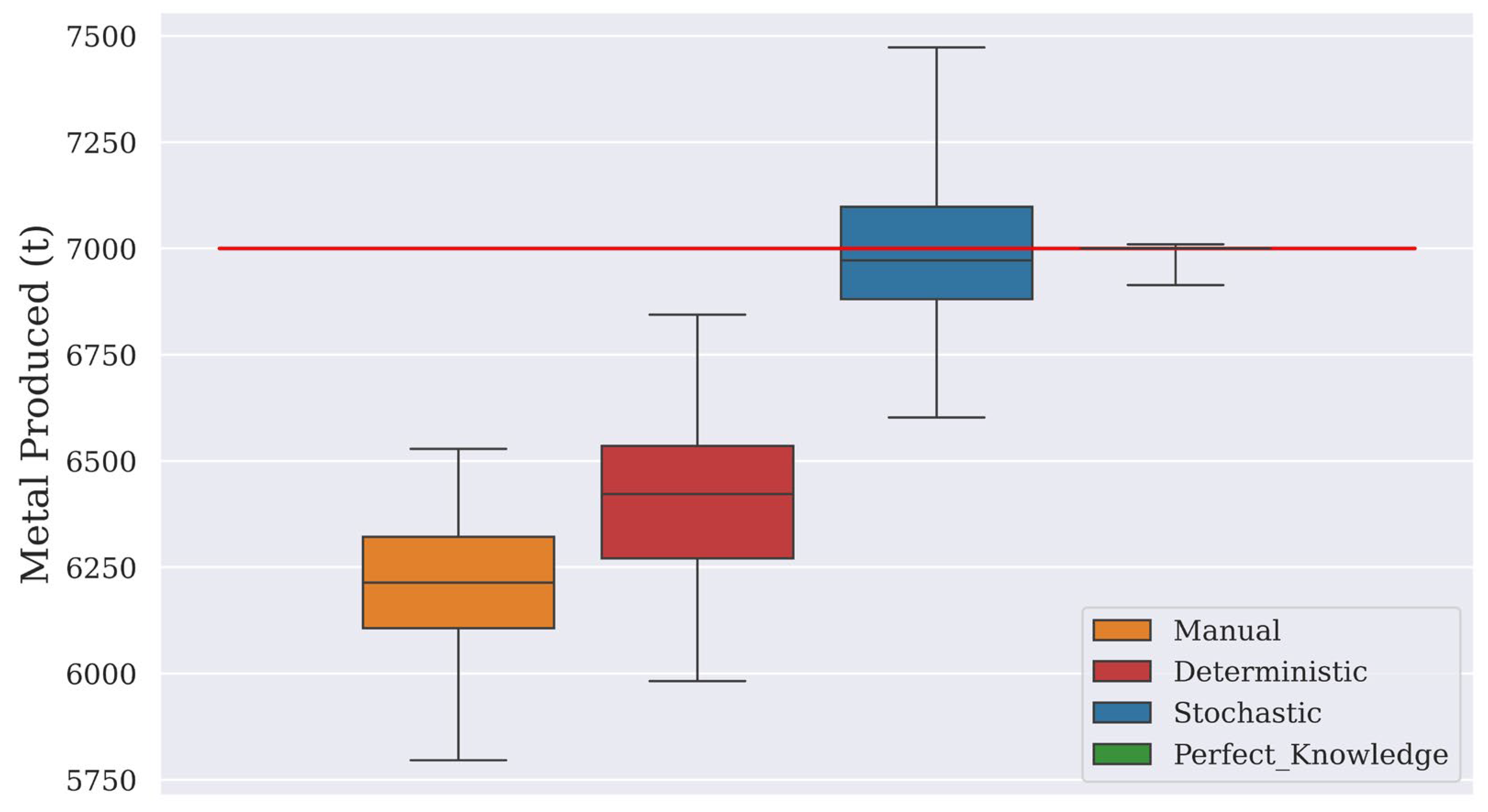
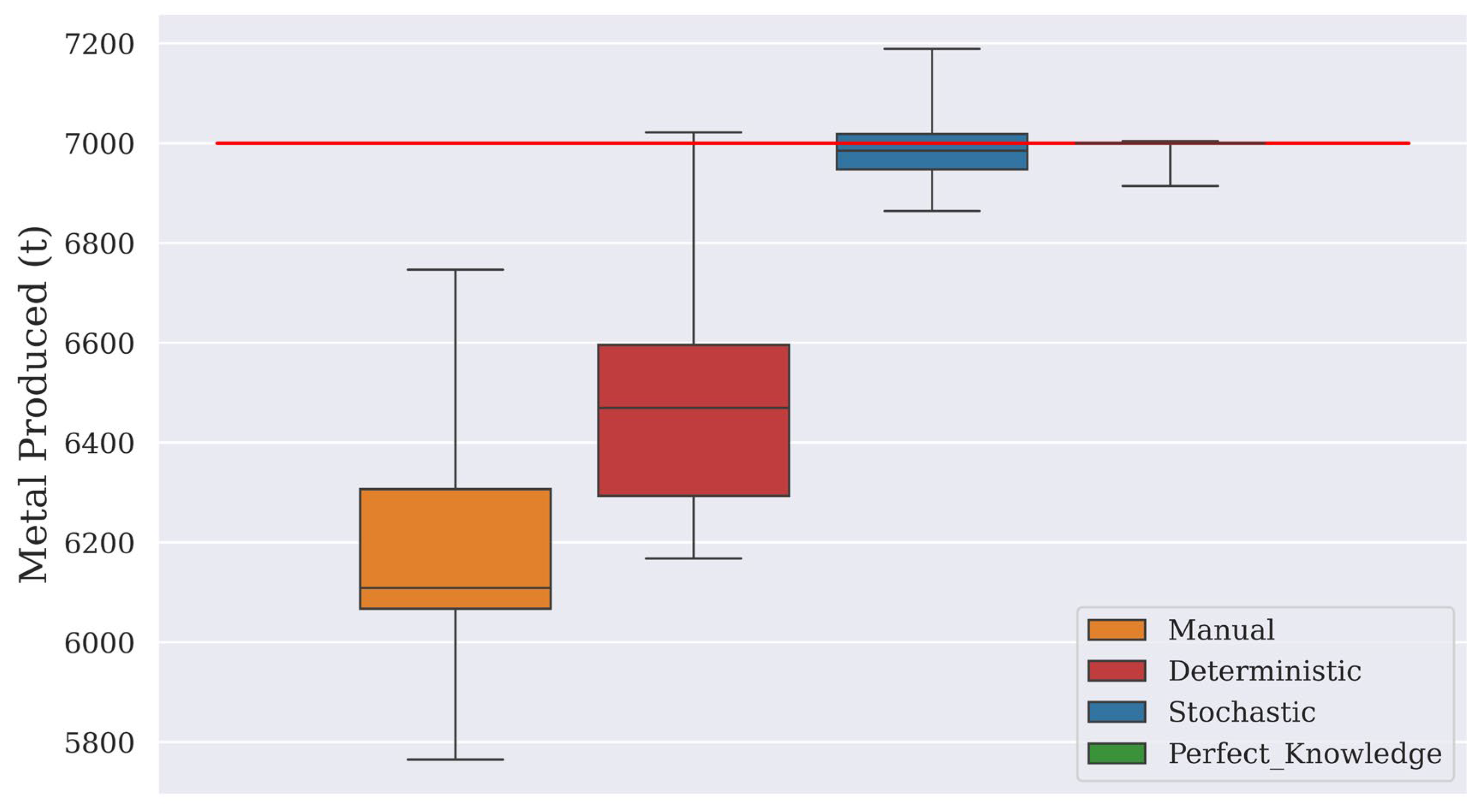
In terms of deviations, Figure 7 presents a boxplot of the production and the required metal target for each definition. As expected, the Stochastic definition complies more closely with the target by adjusting the ore sent to the plant. Both the Deterministic and Manual definitions perform worse in this respect, showing larger average deviations and an overall tendency toward underproduction. In this sense, the inclusion of deviation variables in (ST-DIGOPT) effectively controls metal production across all grade scenarios. Although the average production under the Stochastic definition is close to the 7000 t requirement, some variability persists across scenarios, as a single dig-limit definition cannot perform optimally for every grade simulation. In contrast, the Perfect Knowledge definition can adjust the destination policy independently in each scenario, yielding a much tighter compliance with the target. The Deterministic policy aligns metal production with the kriging estimate, which fails to capture the expected variability, resulting on average in underproduction. The Manual definition also performs poorly in this regard, as adjusting production targets manually is a more cumbersome and imprecise process for the engineer.

For this case study, the Stochastic definition reduces deviation costs by an average of 77% relative to the Deterministic result and by 84% relative to the Manual solution, which highlights the model’s ability to mitigate penalties associated with over- and underproduction across scenarios. Deviation costs are small compared with the profit component of the objective function, and thus the reduction in deviations does not substantially affect overall profit. However, the Stochastic model achieves a better balance between profitability and target compliance, outperforming both the Manual and Deterministic solutions in terms of penalties and profit.

3.2. Case B

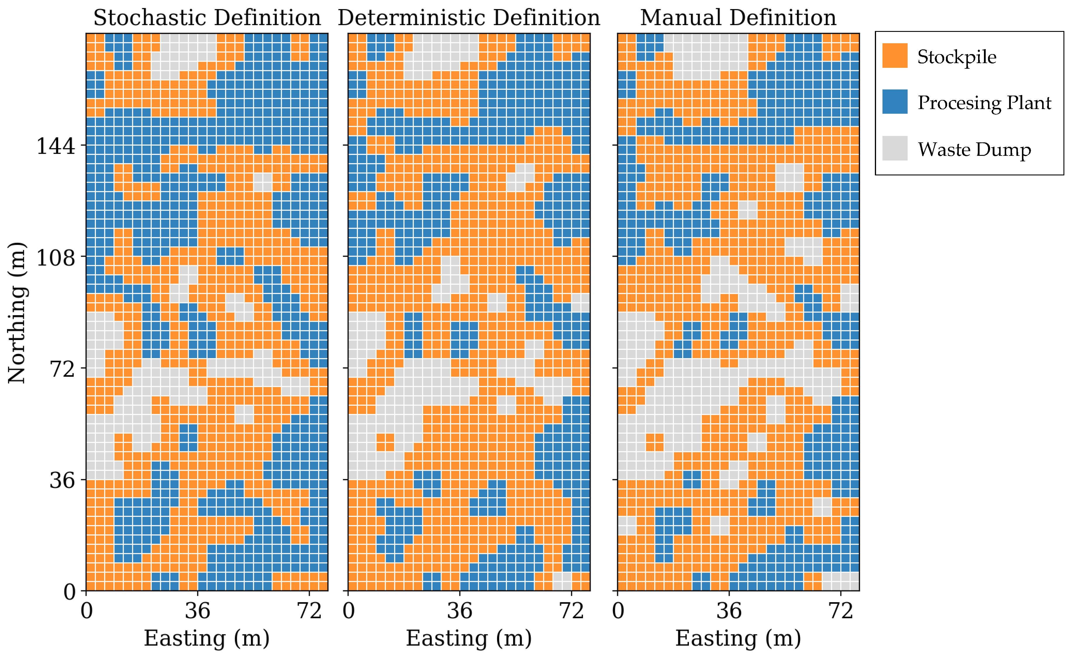
The resulting dig-limit definitions are shown in Figure 8. As in Case A, all definitions fully comply with the minimum selectivity size of 6 × 6 m² imposed for this case study. Although the main zones allocated to plant, stockpile, and waste are broadly consistent, the specific dig-limit contours show notable shifts in each definition. In terms of ore tonnage, the Stochastic definition assigns 268.9 kt to the plant, while the Deterministic variant assigns only 203.6 kt. The Manual definition is closer to the Deterministic solution but even more conservative, allocating just 178.6 kt to the plant. It is important to note that none of the definitions meet the company’s maximum plant capacity of 280 kt, reflecting the low-grade nature of the bench. However, incorporating grade scenarios substantially increases the ore tonnage assigned to the plant, resulting in a more effective utilization of the available processing capacity.

The numerical results for all definitions are presented in

Table 4. Tonnage and average grade by destination for each definition—Case B.

Definition	Waste Dump		Plant		Stockpile
	Tonnage (kt)	Grade (%)	Tonnage (kt)	Grade (%)	Tonnage (kt)	Grade (%)
Deterministic	81.4	0.236 ± 0.006	203.6	0.464 ± 0.006	343.9	0.327 ± 0.004
Stochastic	68.5	0.234 ± 0.007	268.9	0.441 ± 0.005	291.5	0.313 ± 0.004
Perfect Knowledge	93.7 ± 8.9	0.221 ± 0.003	272.5 ± 9.2	0.45 ± 0	262.8 ± 11.2	0.315 ± 0.004
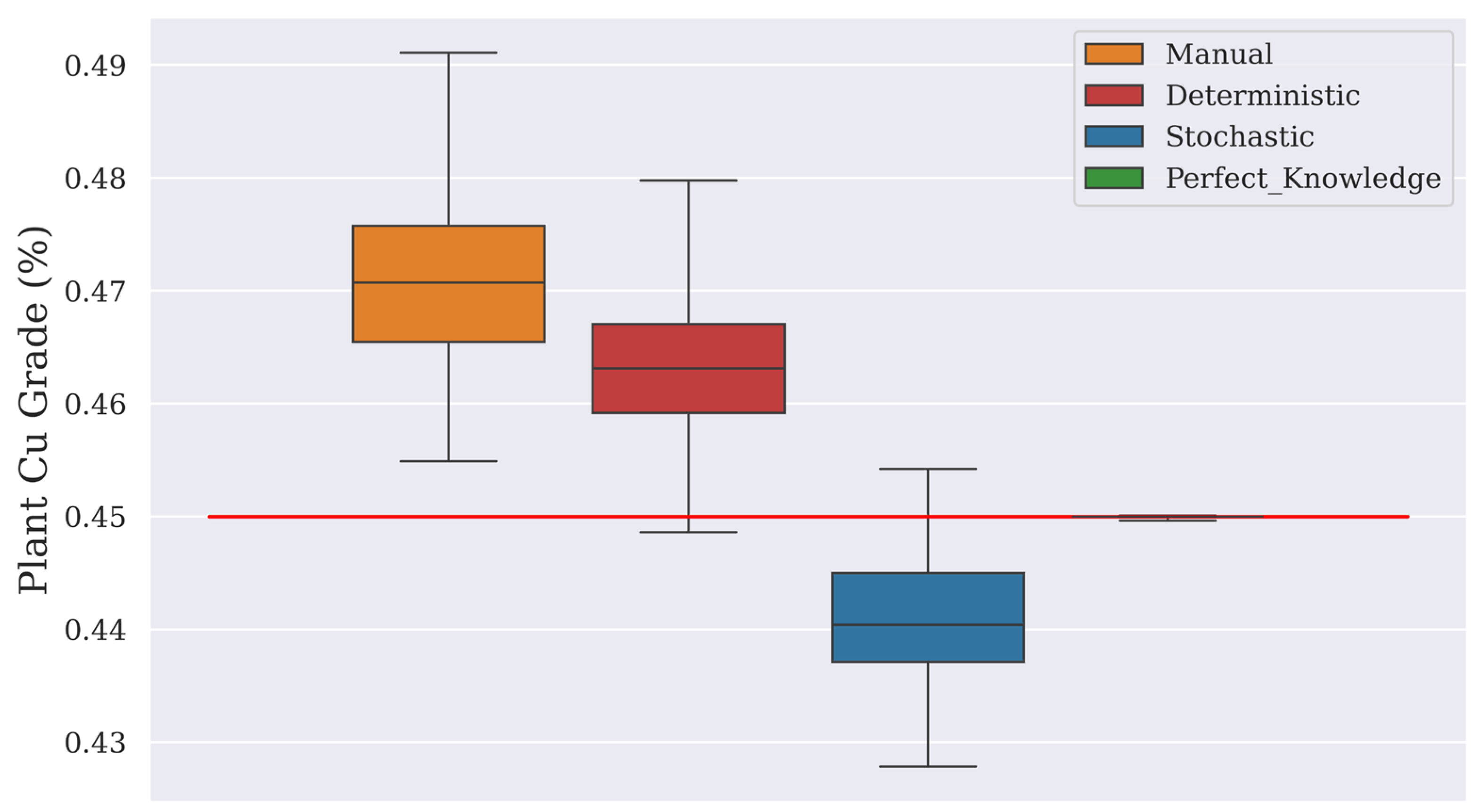
Manual	121.8	0.247 ± 0.005	178.62	0.471 ± 0.007	328.6	0.34 ± 0.004

. The higher ore tonnage assigned to the plant under the Stochastic solution leads to a lower average feed grade across scenarios: 0.441% for the Stochastic solution, compared with 0.464% and 0.471% for the Deterministic and Manual solutions, respectively. By incorporating information from all scenarios, the Stochastic solution prioritizes processing a larger tonnage even at a lower grade, while the other definitions focus on directing only the highest-grade material to the plant based on the estimated scenario.

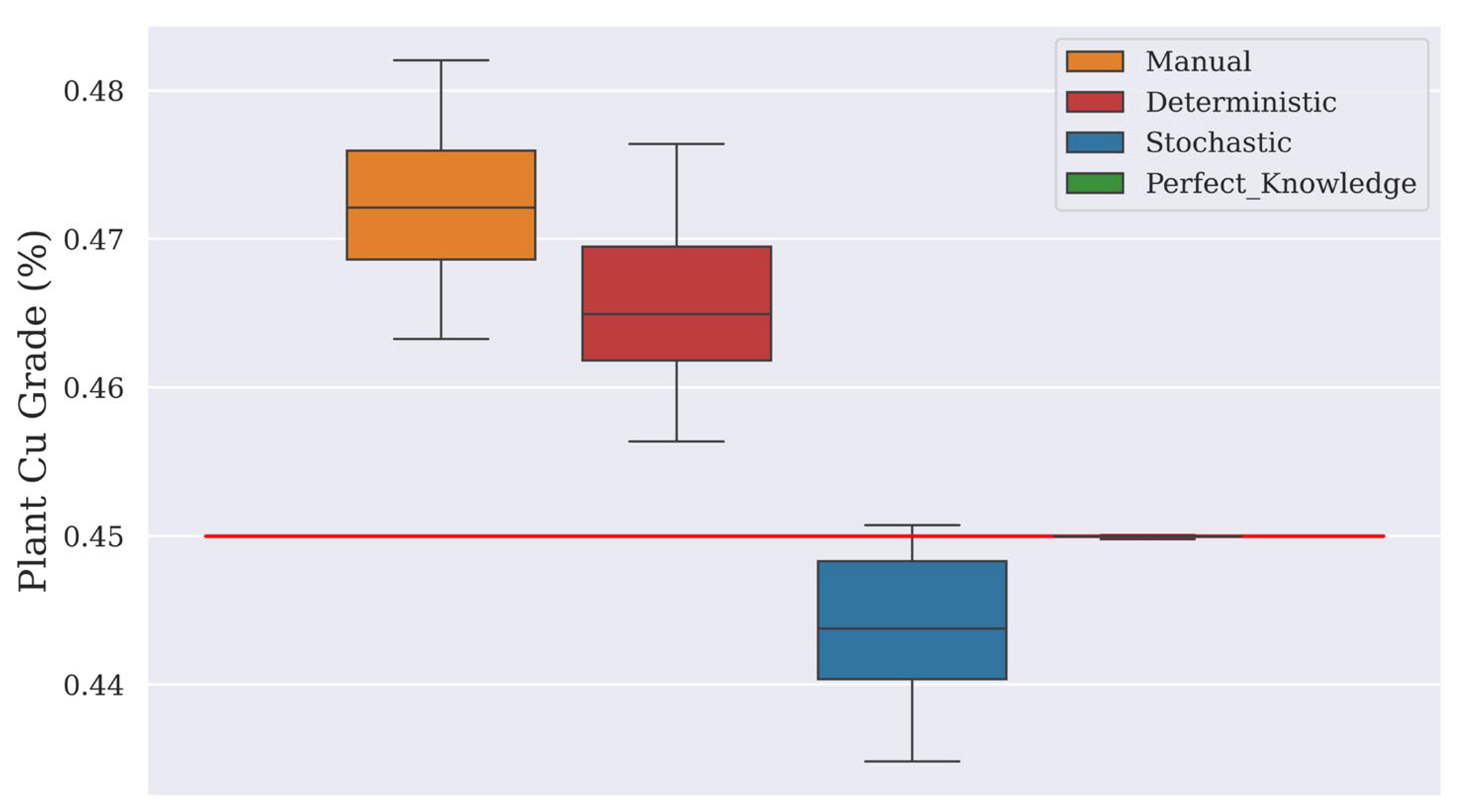
The differences in average grade are also a direct consequence of the production targets defined for this case study, as illustrated in Figure 9. The Stochastic model achieves an average grade that remains close to the 0.45% target, while the Deterministic solution exhibits both higher grades and greater dispersion across scenarios. This behavior stems from the limited information available to the deterministic formulation: the kriging estimate alone does not capture enough grade variability to effectively control deviations across simulations. The Manual solution shows similarly large deviations for the same reason: the estimated scenario obscures the true variability of the deposit. Moreover, the manual procedure depends heavily on the engineer’s judgment, and the common practice of directing the highest-grade material to the plant may conflict with maintaining the target grade across all scenarios.

The stockpile, as the secondary ore destination, serves as a buffer to regulate the average grade and improve the overall profitability of the definitions. Because the plant and stockpile destinations yield similar economic value, directing relatively high-quality material to the stockpile remains a profitable option. All three definitions exploit this alternative to some degree: the Stochastic definition allocates 291.5 kt to the stockpile, compared with 343.9 kt for the Deterministic solution and 328.6 kt for the Manual definition. Notably, even when combining plant and stockpile assignments, the Stochastic definition still yields the highest total ore tonnage at 560.4 kt. Conversely, in terms of waste tonnage, the Stochastic definition assigns the least: only 68.5 kt. In contrast, the Deterministic and Manual definitions send 81.4 kt and 121.7 kt to waste, respectively, with the latter being nearly twice the waste tonnage of the Stochastic definition. This highlights how the additional information contained in the range of grade scenarios enables the optimization model to identify extra ore blocks, increasing the total tonnage processed and stored in this case study.

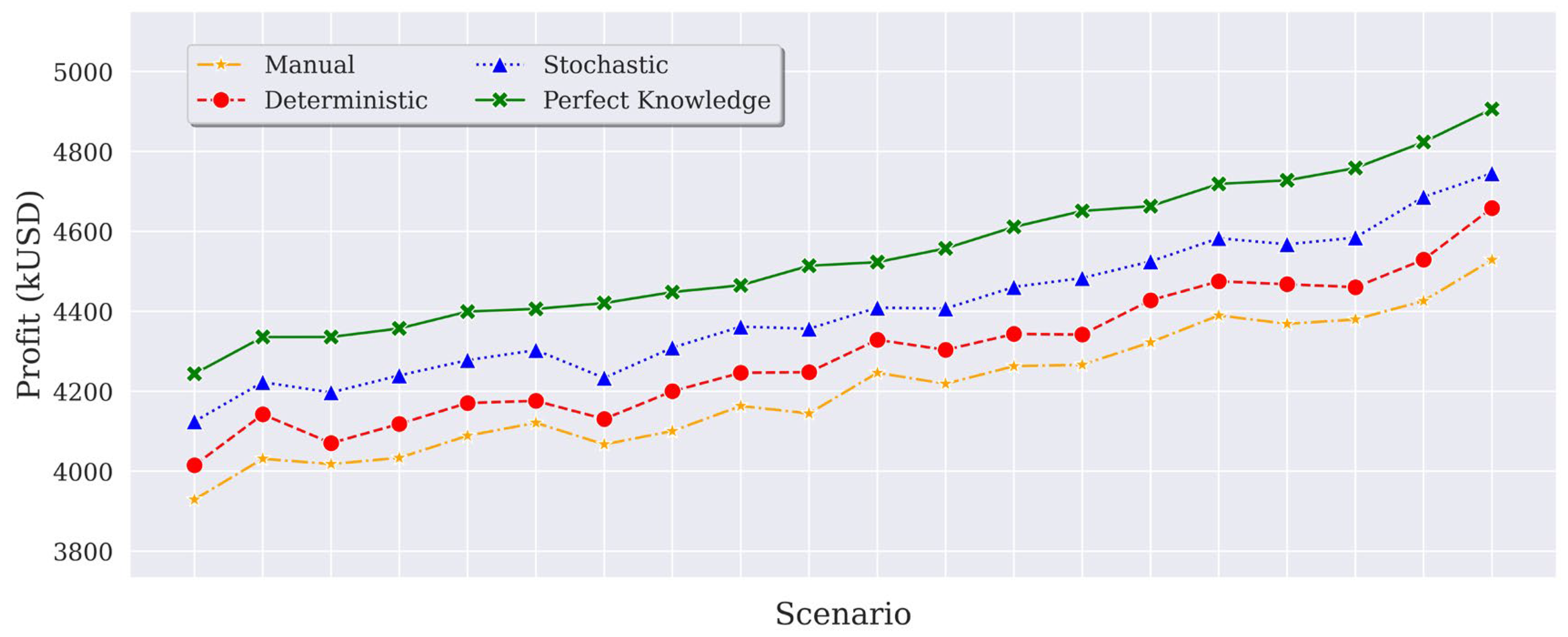
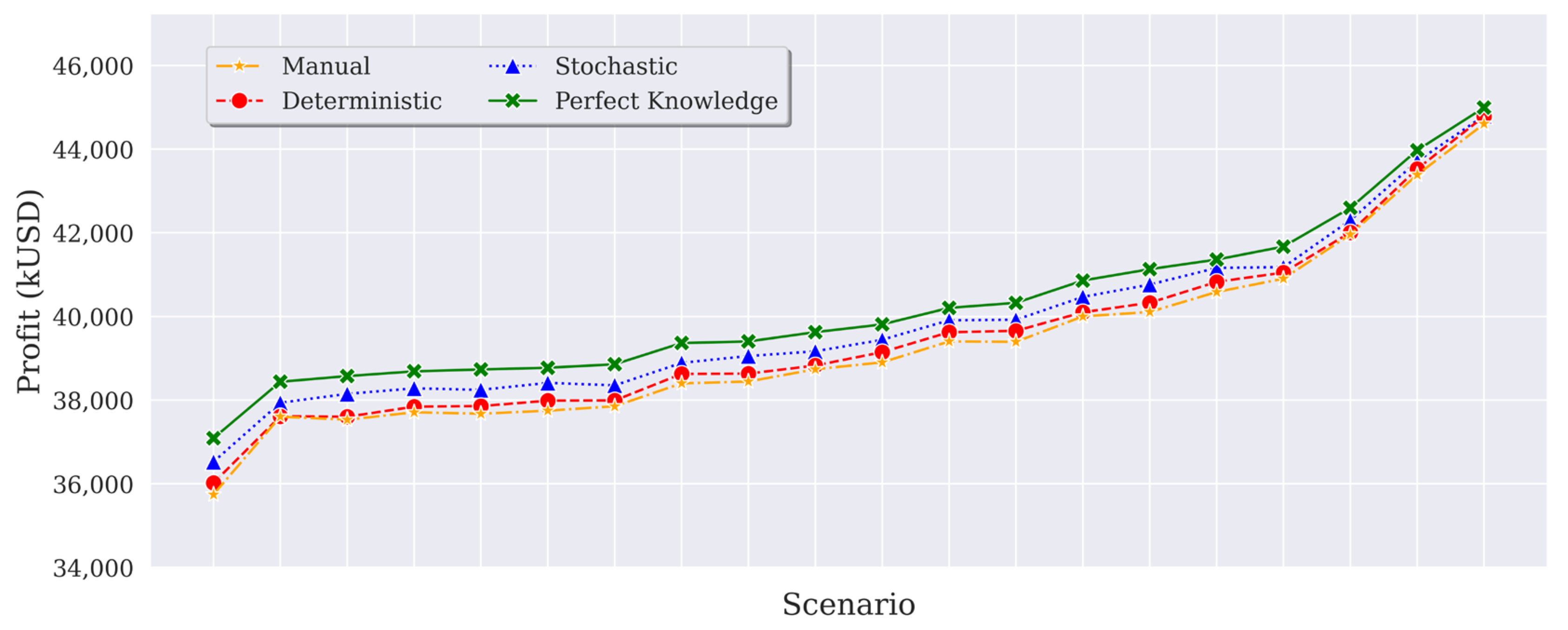
Given that this case study corresponds to a low-grade deposit, even small changes in destination assignment can materially affect economic outcomes. Figure 10 presents the profit distribution for all three definitions across all scenarios, alongside the Perfect Knowledge benchmark.

As shown in Figure 10 and

Table 5. Average profit and deviation costs by definition—Case B.

Definition	Avg. Profit (kUSD)	Avg. Deviation Cost (kUSD)
Deterministic	4251.4 ± 158.3	69.3 ± 31.5
Stochastic	4350.3 ± 160	63.2 ± 32.2
Perfect Knowledge	4491.4 ± 161.2	0.3 ± 0.4
Manual	4172.1 ± 151.7	93.4 ± 30

, the Stochastic definition outperforms both the Deterministic and Manual solutions. Although the profit increases are mostly moderate, they are consistent and statistically significant across scenarios. On average, the deterministic solution provides 1.90% higher profit than the Manual one (p-value: 3.11 × 10⁻⁶³), again highlighting the advantages of optimization-based approaches over manual procedures. The Stochastic solution delivers an additional 2.33% improvement over the deterministic definition (p-value: 5.14 × 10⁻⁸⁷), which further demonstrates that the stochastic model improves economic outcomes even within short-term planning horizons. Overall, the stochastic definition yields a 4.27% higher profit compared to the manual solution (p-value: 5.20 × 10⁻⁸⁸). The higher variability and lower grades of this case study also increase the value of information, which reaches 3.32% (p-value: 3.11 × 10⁻⁶³).

The dispersion in profit across scenarios is also significant in this case study. The difference in profit between the 5th and 95th percentiles ranges from 417.9 kUSD for the deterministic definition to 496.6 kUSD for the Perfect Knowledge definition. These ranges correspond to approximately 10–11% of the mean profit for the respective cases.

Regarding deviation costs, the reduction achieved by the Stochastic formulation is lower than in the previous case study: 8.9% relative to the deterministic solution and 32% relative to the Manual solution. Despite these moderate reductions, the Stochastic formulation still yields higher profit with lower deviations across scenarios, once again outperforming both the Deterministic and Manual definitions.

3.3. Computational Performance and Scenario Sensitivity

In this final section, we analyze the effect of the number of scenarios used in the stochastic formulation on both the computational performance of (ST-DIGOPT) and its results in terms of profit and deviation metrics.

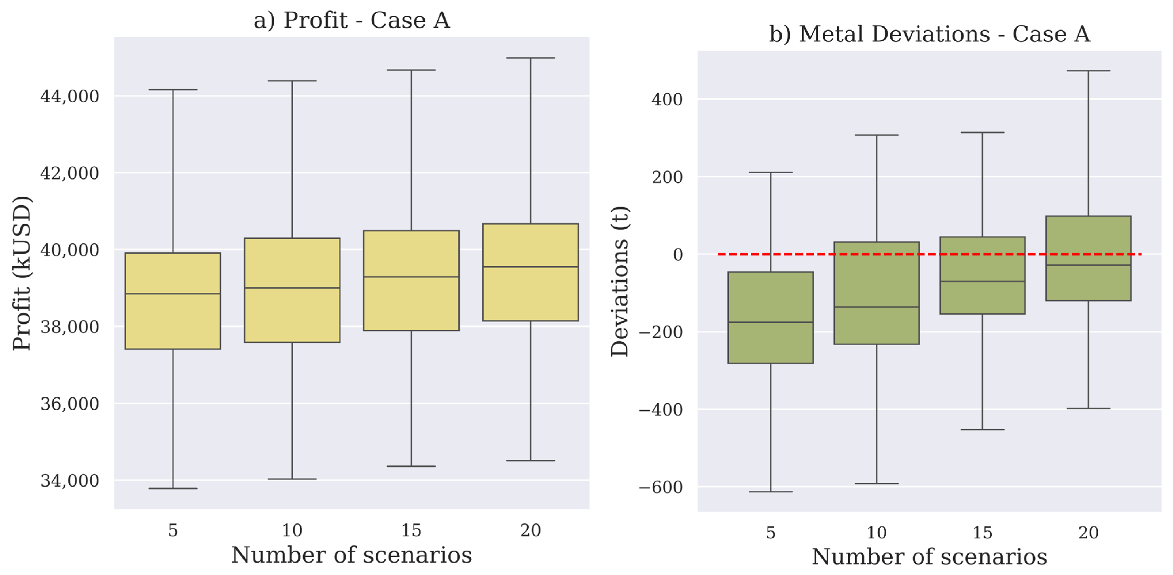
Focusing first on the main performance indicators (expected profit and deviation costs) we analyze case A. Figure 11 shows the distributions of profit and deviations obtained from the stochastic definition using different numbers of scenarios in the training set, with performance evaluated over the testing set, following the same methodology adopted in the previous sections. The figure indicates that increasing the size of the training set leads to modest improvements in economic performance, both in terms of median profit and reduced dispersion across scenarios. This behavior is expected, as a larger training set provides additional information about grade uncertainty, allowing the model to make more informed destination decisions. However, the overall profit improvements achieved with larger training sets are relatively small, reflecting the low level of uncertainty in this case study. While larger sets consistently yield slightly better profitability, the marginal gains remain limited.

In terms of deviations, however, the size of the training set has a clearer impact on target fulfillment in Case A. Metal production deviations tend to be closer to zero as the number of training scenarios increases, indicating that the additional information provided by a larger set of grade realizations improves the model’s ability to control metal production across the testing set.

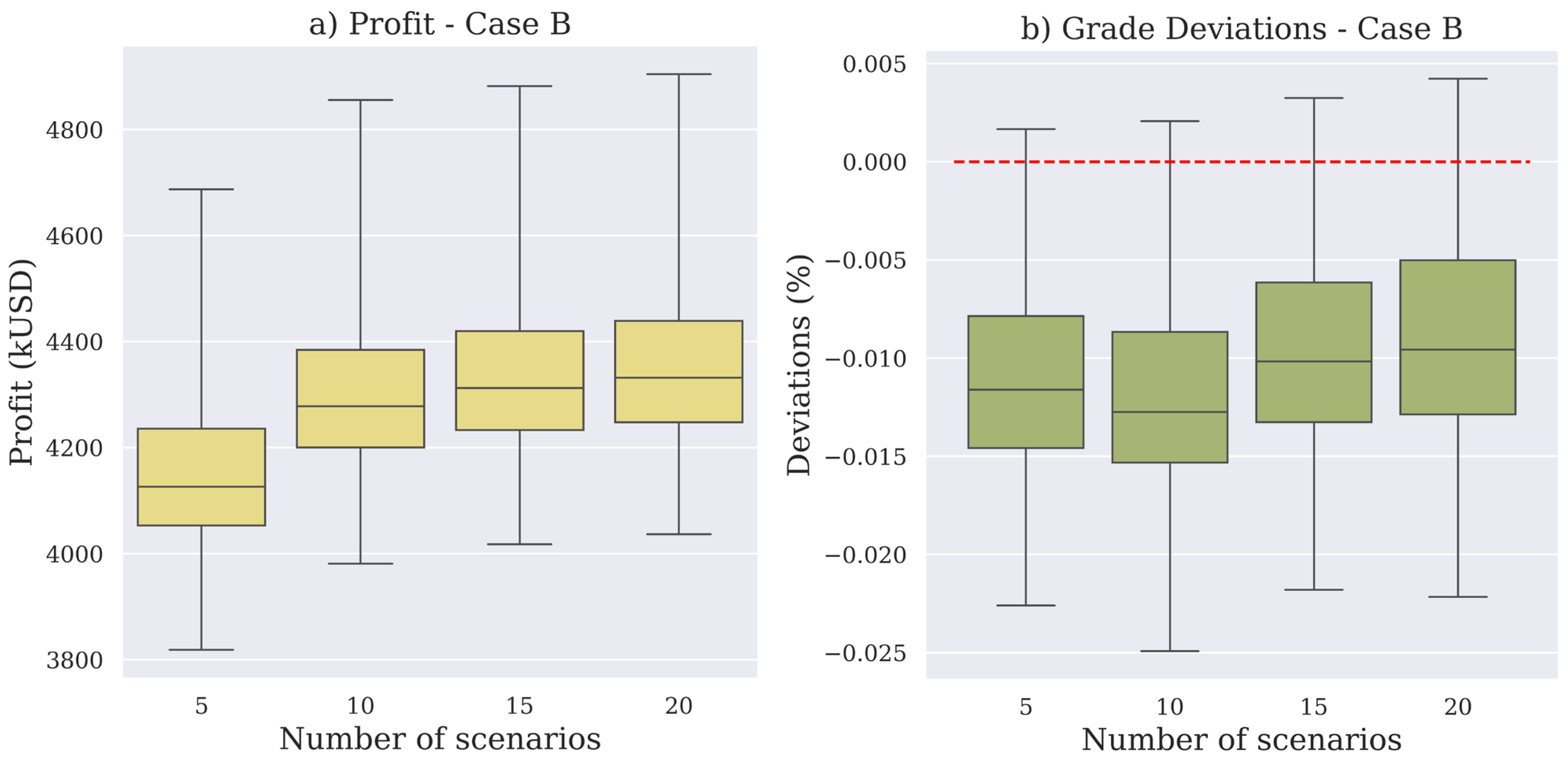
Figure 12 presents the profit and deviation distributions for Case B. In this case, the size of the training set has a more pronounced impact on economic performance. In particular, the median profit increases by nearly 5% when comparing the results obtained with 5 scenarios to those obtained with 20 scenarios. This indicates that, for this case study, the number of scenarios used in the stochastic formulation has a noticeable effect on the profitability of the resulting dig-limit definition. Moreover, the profit tends to stabilize after approximately 15 scenarios, which is expected, as additional scenarios do not necessarily provide new or informative realizations for improving the stochastic decision.

In terms of deviations, the behavior is less systematic than in Case A. Although larger training sets generally lead to improved fulfillment of the target grade, the trend is not as clear or monotonic as for profit. This may be explained by the structure of the objective function, where profit maximization dominates the optimization process, while deviation penalties play a secondary role. As a result, once the model identifies economically favorable destination assignments, further increases in the number of scenarios have a limited impact on reducing deviations.

For both case studies, profit and deviation tend to stabilize with 20 scenarios as the training set. Appendix A presents the results discussed in the previous section but evaluated over the training set. The main performance indicators, including profit and deviations, are similar across both the training and testing sets, further confirming that a training set of 20 scenarios is sufficient for these case studies.

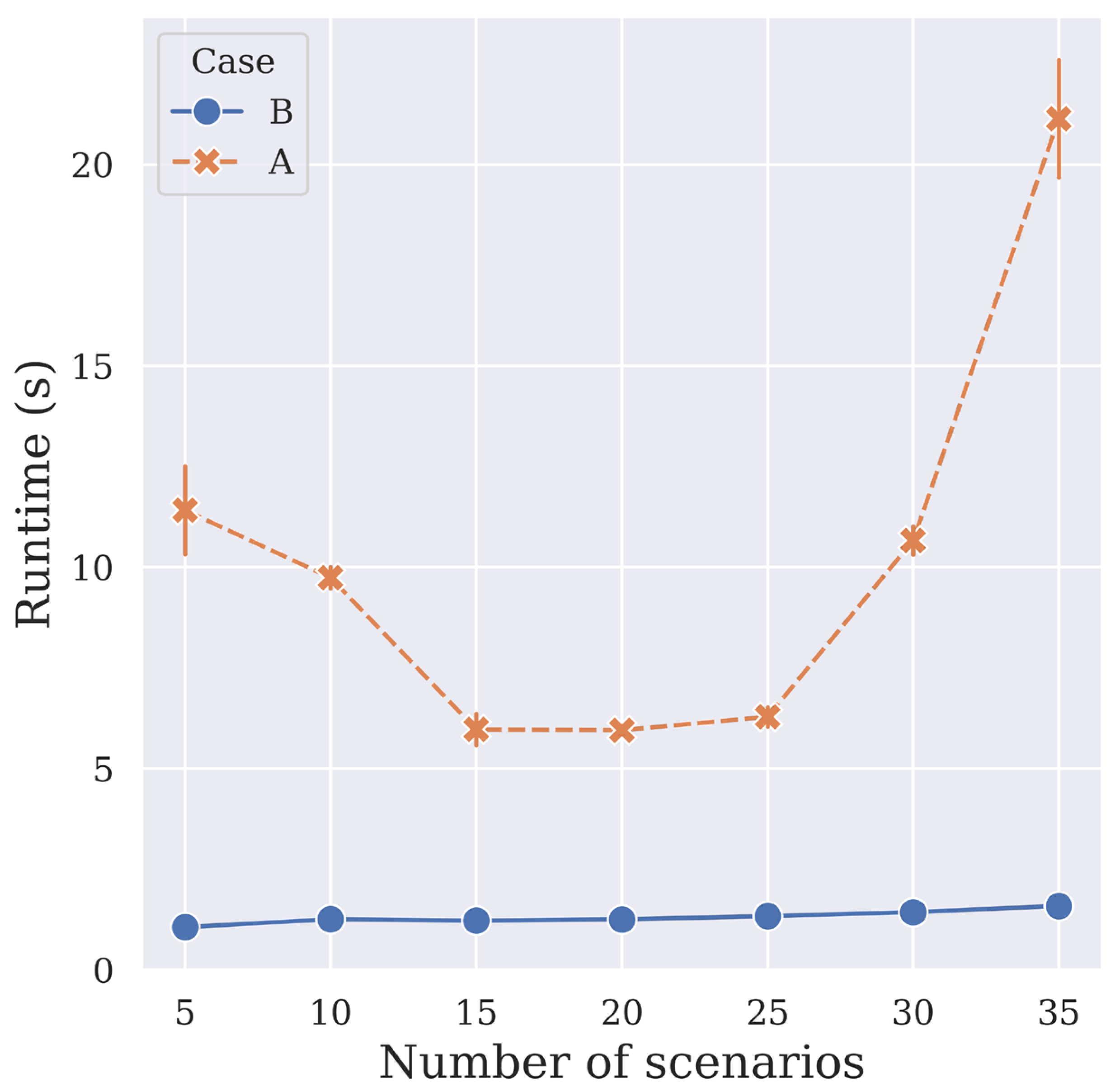
Figure 13 shows the runtime of (ST-DIGOPT) for both case studies as a function of the training set size. As the number of scenarios increases, the number of deviation variables and their associated constraints also increases, as discussed in Section 2, which can raise the computational difficulty of the optimization model and, consequently, the runtime.

For Case B, a mild increasing trend in runtime can be observed as the training set grows; however, the effect is limited, and all instances are solved, on average, in less than 2 s, even for the largest scenario sets. The low runtimes in this case can be explained by the relatively small block model and the small structuring element, both of which have been shown in previous research to have a significant impact on the computational performance of the model. As a reference, the deterministic variant for this case study was solved in 0.63 s, indicating that the stochastic formulation does increase runtimes, although they remain fully compatible with short-term planning requirements.

For Case A, which involves a larger block model, runtimes are overall higher than those observed in Case B. The larger structuring element also contributes to increased computational effort across all configurations. More interestingly, this case study exhibits a non-monotonic runtime pattern. Runtimes tend to decrease as the training set increases from 5 to 20 scenarios and then increase again for larger sets. While unexpected, this behavior can be attributed to the difficulty of solving the dig-limit definition problem under high spatial grade variability. When only a few scenarios are used, the expected block profits tend to exhibit higher spatial variability, which has been shown to increase the complexity of the optimization problem and, consequently, the runtime. As the number of scenarios increases, this variability is smoothed, facilitating the optimization process. However, for even larger training sets, the growing number of deviation variables and associated constraints increases the model complexity, leading to higher runtimes, as expected. For this case study, the deterministic variant also presents higher runtimes than in Case B, reaching an average of 2.24 s.

Overall, all instances for both case studies were solved in less than 25 s, which is fully compatible with the time constraints of short-term planning workflows and significantly faster than a manual dig-limit definition procedure.

4. Discussion

The results indicate that incorporating grade uncertainty can modify destination policies in the dig-limit definition problem. Across both case studies, the proposed stochastic optimization model consistently outperforms both the Manual and Deterministic solutions. However, the magnitude of the additional profit is strongly case-dependent. In settings with higher grade variability and lower average grades, the stochastic model delivers more pronounced economic gains. Conversely, in high-grade benches with lower variability, the benefits of the stochastic formulation are present but comparatively modest.

In both cases, the magnitude of the profit increase is modest but statistically significant. This aligns with previous research showing that stochastic models for copper deposits typically yield low-to-moderate profit improvements over deterministic approaches [18,55,56,75,76]. It is important to note that in short-term planning models, the only available recourse action is controlling deviations from production targets, since both the destination policy and the extraction sequence are fixed. By contrast, long-term models can exploit grade scenarios to adjust not only destination decisions but also the extraction sequence, which often leads to greater economic gains. Even so, the results presented here demonstrate that meaningful advantages can still be obtained from stochastic definitions in the short-term horizon. Moreover, in deposits where additional sources of uncertainty (rock type, alteration, or other geological variables) play a significant role, the stochastic framework proposed in this work could yield larger benefits.

The stochastic model also controls deviations from production targets more effectively than both the Manual and Deterministic policies. The ability to regulate grade or metal production across a range of scenarios can influence operational performance in ways that extend beyond profit or deviation costs alone. For instance, plant performance depends on achieving expected grade targets, which are typically set to maximize metallurgical recovery. Deviations from these targets may directly affect the actual metal recovered, offering an additional advantage to the stochastic approach. Similarly, maintaining steady metal production is often tied to long-term planning objectives, where failure to meet targets can incur penalties or generate extra costs associated with rehandling material. In all these respects, the stochastic formulation provides a more reliable and consistent destination policy.

The deterministic version of the dig-limit definition problem is known to suffer from long runtimes, particularly when larger structuring elements are used [10,11]. Our implementation of (ST-DIGOPT) extends a previously developed deterministic variant that has been shown to be computationally efficient, and the stochastic extension follows the same trend. Although the stochastic formulation is more computationally demanding than the deterministic variant in both case studies, all runtimes remain fully compatible with short-term planning horizons.

Runtimes are also influenced by the heterogeneity of the grade distribution and the block model size. This effect is more pronounced in Case A, where smaller training sets tend to produce longer runtimes than medium-sized sets. This behavior can be attributed to the higher spatial variability present in the bench when only a limited number of scenarios is considered, relative to the averaged profit obtained with larger training sets in the stochastic formulation and the smoothed kriging estimate used in the deterministic model. This observation is further reinforced by the performance of the Perfect Knowledge definition, which required substantially longer runtimes, with an average of 42 s and a standard deviation of 31.59 s. This indicates that the most challenging instances arise from high spatial variability in the grade distribution, while the large dispersion suggests that computational difficulty is highly scenario dependent. Overall, these results indicate that the complexity of the optimization problem is driven primarily by the spatial variability of the grade realization, and secondarily by the size of the block model and the structuring element. This finding is consistent with previous research, where increased spatial variability has been shown to significantly impact the complexity and runtime of similar optimization problems [77].

The evaluation using the training set of the stochastic policy is virtually indistinguishable from the testing set in terms of both average profit and deviations (Appendix A). This indicates that the use of 20 scenarios is adequate for the short-term planning horizon and for the level of variability present in these case studies, which aligns with previous research on stochastic models for short-term mine planning. Given that the model remains computationally efficient, increasing the number of scenarios is feasible in contexts where higher geological variability is expected. This may be particularly relevant when incorporating additional sources of grade uncertainty that have gained traction in the recent literature, such as rock type, geometallurgical responses, or blast-induced movement. As long as the underlying uncertainty can be represented through grade or profit scenarios, the proposed framework is flexible enough to accommodate it. This flexibility could help identify which source of uncertainty is most critical within this planning horizon. However, the proposed model does not account for other sources of uncertainty, such as truck and shovel productivity, which can significantly affect ore and waste production targets and have been incorporated into previous short-term planning models [60,61]. Consequently, an important avenue for future research is the integration of equipment productivity uncertainty into the dig-limit definition problem, with the aim of further improving target compliance in short-term planning horizons.

The minimization-of-deviations framework requires the specification of deviation cost parameters. The most common approach in the literature relies on a trial-and-error process to balance expected profit and compliance with production targets. In this work, we followed a similar procedure, adjusting the deviation costs for each case study until both the deterministic and stochastic formulations achieved an acceptable level of target control. However, this process is manual and dependent on expert judgment, which constitutes a limitation of the proposed approach. While previous studies have analyzed the impact of deviation costs in planning problems under uncertainty [72,78], there are still no clear guidelines for selecting these parameters systematically. Future research could focus on developing objective criteria for setting deviation costs based on the relative importance and economic consequences of deviations from the desired targets.

Finally, our results indicate that even in case studies with relatively low variability, the distribution of profit exhibits a wide range of outcomes across scenarios, with differences ranging between 10% and 15% of the average profit across dig-limit definitions. Since the proposed model is risk-neutral, all scenarios are weighted equally, and no particular emphasis is placed on adverse cases. Several risk-averse and robust optimization approaches have been proposed in the literature to address this limitation [17,18]. Future research could therefore focus on extending the stochastic framework to incorporate risk-averse criteria, enabling the formulation of dig-limit definitions that explicitly account for downside risk and deliver more stable economic performance, with a higher probability of target compliance under unfavorable scenarios.

5. Conclusions

Our work introduced a novel stochastic optimization model for dig-limit definition problem that incorporates grade uncertainty through multiple geological scenarios. Across two case studies, the proposed formulation consistently outperformed both deterministic and manual approaches. Although the profit gains were generally modest, they were statistically significant and more pronounced in low-grade, high-variability settings.

The stochastic solutions also provided better control of production targets, reducing deviations in metal output and achieving more stable grades across scenarios. This improved reliability is valuable for short-term planning where fluctuations can affect plant performance, recovery, and long-term production goals.

The results show that considering grade variability can enhance short-term destination policies, offering both economic and operational benefits. Future work may extend the framework toward equipment performance uncertainty and risk-averse formulations to further improve robustness under uncertainty.