Scrutinizing the General Conic Equation

Abstract

We present a general formula that transforms any conic of the form $A{x}^2+Bxy+C{y}^2+Dx+Ey+F=0$, with $B\ne 0$, into $A^{\prime }{\left(x^{\prime }\right)}^2+C^{\prime }{\left(y^{\prime }\right)}^2+D^{\prime }{x}^{\prime }+E^{\prime }{y}^{\prime }+F=0$, without requiring the rotation angle $\theta$. This directly eliminates the cross term $xy$, simplifying the rotated conics analysis. As consequences, we obtain new formulae that remove both rotations and translations, a novel proof of the discriminant criterion, improved expressions for eccentricity, and a detailed taxonomy of all loci described by the general conic equation.

1. Introduction

Analytic Geometry is often relegated to secondary status, primarily serving pedagogical purposes in pre-calculus courses. Consequently, classical methods for eliminating the cross term $xy$ in the general conic equation

$$A{x}^2+Bxy+C{y}^2+Dx+Ey+F=0$$

(1)

with $B\ne 0$, remain largely unquestioned. Traditionally, this involves applying a rotation of axes to express the conic as

$$A^{\prime }{\left(x^{\prime }\right)}^2+C^{\prime }{\left(y^{\prime }\right)}^2+D^{\prime }{x}^{\prime }+E^{\prime }{y}^{\prime }+F=0.$$

(2)

This reduction is achieved via the standard rotation transformations:

$$\begin{array}{ccc}\hfill x& =& x^{\prime }cos\theta -y^{\prime }sin\theta ,\hfill \end{array}$$

(3)

$$\begin{array}{ccc}\hfill y& =& x^{\prime }sin\theta +y^{\prime }cos\theta ,\hfill \end{array}$$

(4)

where $\theta \in ]0,\pi /2[$ is chosen to nullify the $xy$-term. This approach is universally presented in classical texts (see p. 68 in [1], p. 141 in [2], p. 138 in [3], pp. 186-187 in [4], Chapters 5.3 and 7.5 in [5], and Chapter 1 in [6]), presuming the necessity of the rotation angle $\theta$ in every instance of the process of transforming (1) into (2).

Theorem 1

(First Theorem of the Rotation Angle). Let $A,B,C,D,E,F\in \mathbb{R}$ be such that (1) represents a locus in ${\mathbb{R}}^2$ different from any single straight line and any circumference (degenerate or not). If this conic is generated by a rotation angle $\theta \in ]0,\pi /2[$, then $B\ne 0$, and also

(i) $A=C$ if and only if $\theta =\pi /4$,

(ii)  $\theta \in ]0,\pi /4[\cup ]\pi /4,\pi /2[$ if and only if $tan\left(2\theta \right)={\displaystyle \frac{B}{A-C}}$.

Plugging x and y from (3) and (4) into (1) yields (2). To illustrate this process, consider the following three examples.

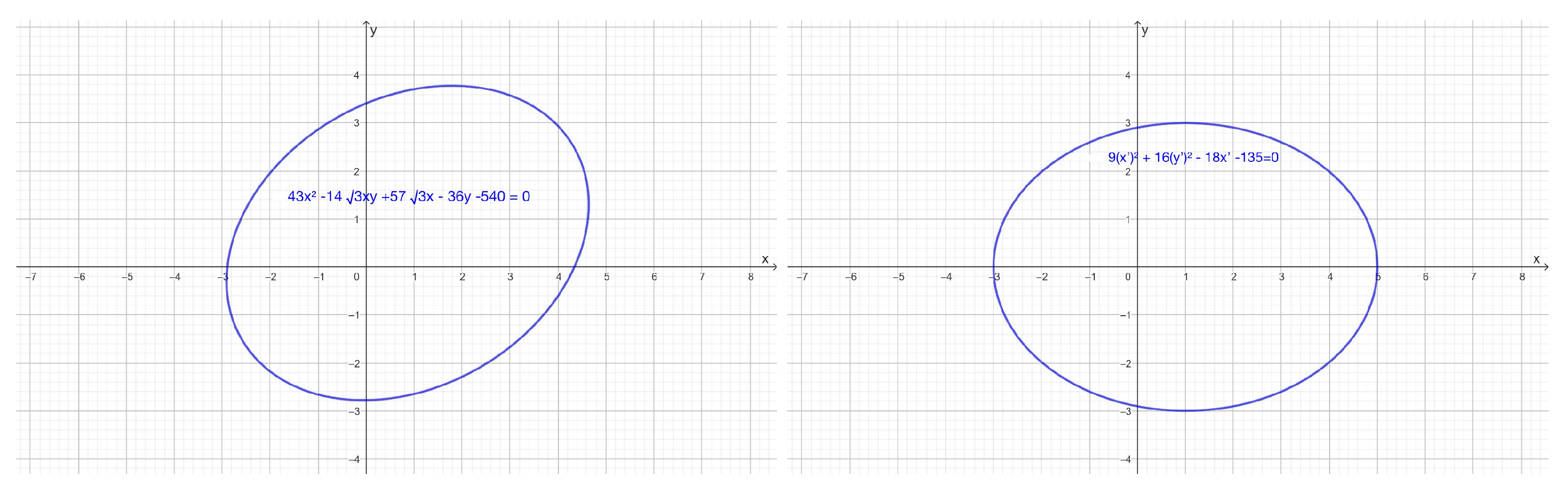
Example 1.

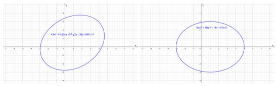
If $43x^2-14\sqrt{3}xy+57y^2-36\sqrt{3}x-36y-540=0$, then Theorem 1 implies that $\theta ={\displaystyle \frac{1}{2}}arctan\left({\displaystyle \frac{B}{A-C}}\right)={\displaystyle \frac{1}{2}}arctan\left(-{\displaystyle \frac{14\sqrt{3}}{43-57}}\right)={30}^{\circ },$ so $sin\theta =sin{30}^{\circ }={\displaystyle \frac{1}{2}}$ and $cos\theta =cos{30}^{\circ }={\displaystyle \frac{\sqrt{3}}{2}}$; hence, (3)–(4) imply $x={\displaystyle \frac{\sqrt{3}{x}^{\prime }-y^{\prime }}{2}}$ and $y={\displaystyle \frac{(x^{\prime }+\sqrt{3}{y}^{\prime })}{2}}.$ Thus: $43{\left({\displaystyle \frac{\sqrt{3}{x}^{\prime }-y^{\prime }}{2}}\right)}^2-14\sqrt{3}{\displaystyle \frac{\sqrt{3}{x}^{\prime }-y^{\prime }}{2}}{\displaystyle \frac{x^{\prime }+\sqrt{3}{y}^{\prime }}{2}}+57{\left({\displaystyle \frac{x^{\prime }+\sqrt{3}{y}^{\prime }}{2}}\right)}^2-36\sqrt{3}{\displaystyle \frac{\sqrt{3}{x}^{\prime }-y^{\prime }}{2}}-36{\displaystyle \frac{x^{\prime }+\sqrt{3}{y}^{\prime }}{2}}-540=0$, and after several (and busy) algebraic manipulations, we obtain $9{\left(x^{\prime }\right)}^2+16{\left(y^{\prime }\right)}^2-18x^{\prime }-135=0$. Therefore, the given equation corresponds to the general equation of a rotated ellipse whose canonical form without rotations is ${\displaystyle \frac{{(x^{\prime }-1)}^2}{16}}+{\displaystyle \frac{{\left(y^{\prime }\right)}^2}{9}}=1.$ See Figure 1.

Figure 1. Plots from Example 1: $43x^2-14\sqrt{3}xy+57y^2-36\sqrt{3}x-36y-540=0$ (on the left) and $9{\left(x^{\prime }\right)}^2+16{\left(y^{\prime }\right)}^2-18x^{\prime }-135=0$ (on the right).

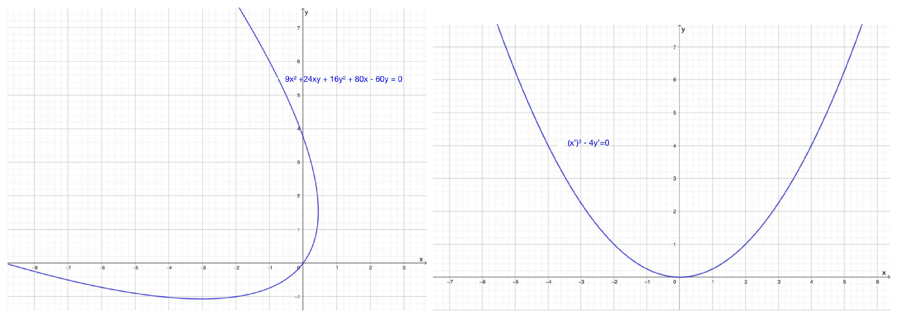
Example 2.

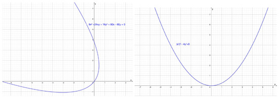
If $9x^2+24xy+16y^2+80x-60y=0$, then, by Theorem 1, $tan\left(2\theta \right)={\displaystyle \frac{24}{9-16}}=-{\displaystyle \frac{24}{7}}$ and $\theta ={\displaystyle \frac{1}{2}}arctan\left(-{\displaystyle \frac{24}{7}}\right)\approx 53.{13}^{\circ }$. So, if the two trigonometric identities $sin\alpha =\sqrt{{\displaystyle \frac{1}{2}}\left(1+{\displaystyle \frac{1}{\sqrt{1+{tan}^2\left(2\alpha \right)}}}\right)}$ and $cos\alpha =\sqrt{{\displaystyle \frac{1}{2}}\left(1-{\displaystyle \frac{1}{\sqrt{1+{tan}^2\left(2\alpha \right)}}}\right)}$ hold for $\theta \in \left]{\displaystyle \frac{\pi }{4}},{\displaystyle \frac{\pi }{2}}\right]$ (see [7] [Chapter 7]), then $tan\left(2\theta \right)=-{\displaystyle \frac{24}{7}}$, which implies that $sin\theta ={\displaystyle \frac{4}{5}}$ and $cos\theta ={\displaystyle \frac{3}{5}}$. Hence, (3) and (4) yield $x={\displaystyle \frac{3x^{\prime }-4y^{\prime }}{5}}$ and $y={\displaystyle \frac{4x^{\prime }+3y^{\prime }}{5}}$. Thus, $9{\left({\displaystyle \frac{3x^{\prime }-4y^{\prime }}{5}}\right)}^2+24{\displaystyle \frac{3x^{\prime }-4y^{\prime }}{5}}{\displaystyle \frac{4x^{\prime }+3y^{\prime }}{5}}+16{\left({\displaystyle \frac{4x^{\prime }+3y^{\prime }}{5}}\right)}^2+80{\displaystyle \frac{3x^{\prime }-4y^{\prime }}{5}}-60{\displaystyle \frac{4x^{\prime }+3y^{\prime }}{5}}=0$, which, after many tedious algebraic calculations, is reduced to ${\left(x^{\prime }\right)}^2-4y^{\prime }=0$. Therefore, the given equation corresponds to a rotated parabola whose vertex coincides with the origin of the Cartesian plane (see Figure 2).

Figure 2. Plots from Example 2: $9x^2+24xy+16y^2+80x-60y=0$ (on the left) and ${\left(x^{\prime }\right)}^2-4y^{\prime }=0$ (on the right).

Example 3.

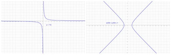
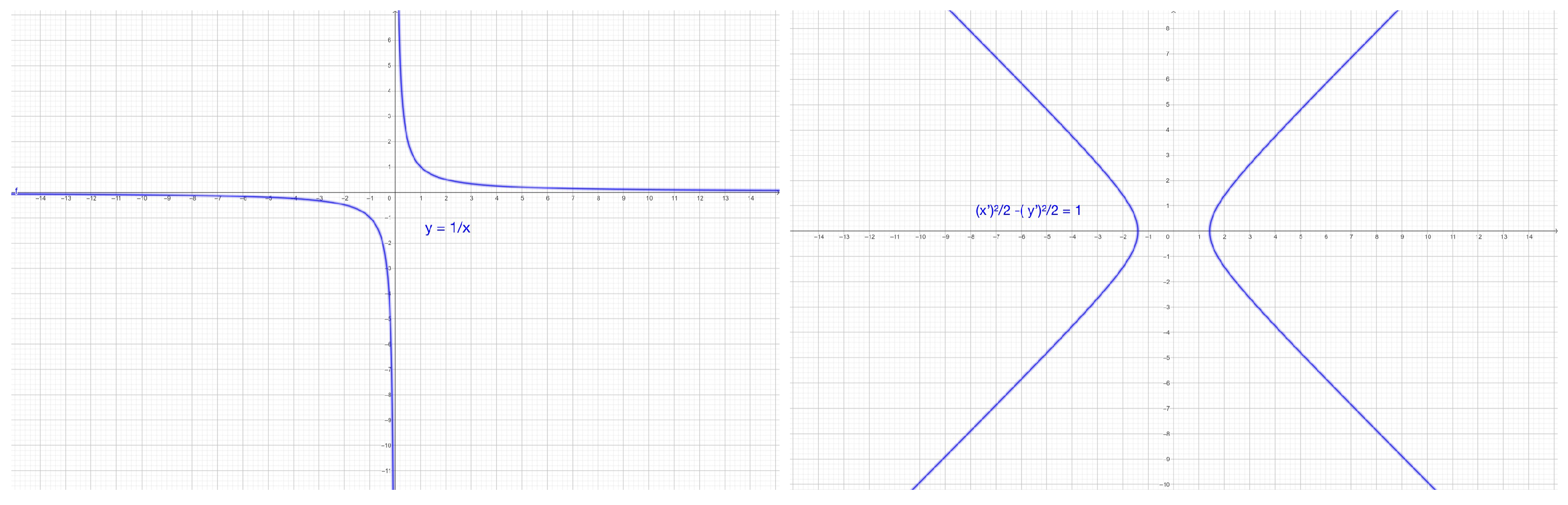
If $y={\displaystyle \frac{1}{x}}$, then $xy-1=0$ and Theorem 1 implies $\theta ={45}^{\circ }$ due to the fact that $A=C=0$, so $sin\theta =sin{45}^{\circ }=cos\theta =cos{45}^{\circ }={\displaystyle \frac{\sqrt{2}}{2}}$. Hence, by (3) and (4), we have that $x={\displaystyle \frac{\sqrt{2}{x}^{\prime }-\sqrt{2}{y}^{\prime }}{2}}$ and $y={\displaystyle \frac{\sqrt{2}{x}^{\prime }+\sqrt{2}{y}^{\prime }}{2}}$; thus, ${\displaystyle \frac{\sqrt{2}{x}^{\prime }-\sqrt{2}{y}^{\prime }}{2}}{\displaystyle \frac{\sqrt{2}{x}^{\prime }+\sqrt{2}{y}^{\prime }}{2}}-1=0,$ which is reduced to ${\displaystyle \frac{{\left(x^{\prime }\right)}^2}{2}}-{\displaystyle \frac{{\left(y^{\prime }\right)}^2}{2}}=1$. Therefore, the given equation corresponds to the general equation of a rotated equilateral hyperbola (see Figure 3).

Figure 3. Plots from Example 3: $y={\displaystyle \frac{1}{x}}$ (on the left) and ${\displaystyle \frac{{\left(x^{\prime }\right)}^2}{2}}-{\displaystyle \frac{{\left(y^{\prime }\right)}^2}{2}}=1$ (on the right).

Despite advances in computational tools, students often find the algebraic manipulations in analytic geometry, such as those in Examples 1–3, tedious. This paper introduces a more efficient approach to these problems via a new result of general applicability.

The structure is as follows: Section 2 outlines the necessary preliminaries. Section 3 presents our main contribution, Theorem 3, along with related results. In Section 4, we apply Theorem 3 to revisit classical results and examine special and degenerate cases. Section 5 addresses the instant simplification of the general conic equation under rotations and translations. Section 6 explores further properties of conics, including eccentricity, and a full taxonomy in ${\mathbb{R}}^2$. We conclude with a brief discussion in Section 7.

2. Preliminaries

It is important to briefly review some important known facts related to (1) and other mathematical tools.

2.1. Properties of the General Conic Equation and the Sign Function

We start by considering that if (3) and (4) are substituted in (1), we obtain

$$\begin{array}{c}\hfill \left(A{cos}^2\theta +Bsin\theta cos\theta +C{sin}^2\theta \right){\left(x^{\prime }\right)}^2+\left[B\left({cos}^2\theta -{sin}^2\theta \right)-2(A-C)sin\theta cos\theta \right]x^{\prime }{y}^{\prime }\\ \hfill +\left(A{sin}^2\theta -Bsin\theta cos\theta +C{cos}^2\theta \right){\left(y^{\prime }\right)}^2+(Dcos\theta +Esin\theta )x^{\prime }+(-Dsin\theta +Ecos\theta )y^{\prime }+F=0\end{array}$$

(5)

(see p. 213 in [2]). The importance of the former expression lies in the fact that it is identical to (2) member to member, which implies the following four relations:

$$\begin{array}{ccc}\hfill A^{\prime }& =& A{cos}^2\theta +Bsin\theta cos\theta +C{sin}^2\theta ,\hfill \end{array}$$

(6)

$$\begin{array}{ccc}\hfill C^{\prime }& =& A{sin}^2\theta -Bsin\theta cos\theta +C{cos}^2\theta ,\hfill \end{array}$$

(7)

$$\begin{array}{ccc}\hfill D^{\prime }& =& Dcos\theta +Esin\theta ,\hfill \end{array}$$

(8)

$$\begin{array}{ccc}\hfill E^{\prime }& =& -Dsin\theta +Ecos\theta .\hfill \end{array}$$

(9)

In addition, (5) and Theorem 1 guarantee $B^{\prime }=B\left({cos}^2\theta -{sin}^2\theta \right)-2(A-C)sin\theta cos\theta =Bcos\left(2\theta \right)-(A-C)sin\left(2\theta \right)=0.$ Meanwhile, (1), (2), and (5) have the same independent term F. On the other hand, consider the sign function, which, according to p. 378 in [8], is defined for all $a\in \mathbb{R}$ as follows:

$$\mathrm{sgn}\left(a\right):=\left\{\begin{array}{cc}-1,& \mathrm{i}\mathrm{f} a<0\\ 0,& \mathrm{i}\mathrm{f} a=0\\ 1,& \mathrm{i}\mathrm{f} a>0.\end{array}\right.$$

(10)

This definition implies the following properties of the sign function:

• Property 1: $a=\left|a\right|·\mathrm{sgn}\left(a\right) \mathrm{for}\mathrm{all} a\in \mathbb{R}$,
• Property 2: $\left|a\right|=a·\mathrm{sgn}\left(a\right) \mathrm{for}\mathrm{all} a\in \mathbb{R}$,
• Property 3: ${\mathrm{sgn}}^2\left(a\right)=1 \mathrm{for}\mathrm{all} a\in \mathbb{R}\setminus \left\{0\right\}$.

Finally, let us consider the definition of the matrix of the quadratic equation (see, for instance, p. 30 in [9]), which is given as $Q:=\left(\begin{array}{ccc}A& {\displaystyle \frac{B}{2}}& {\displaystyle \frac{D}{2}}\\ {\displaystyle \frac{B}{2}}& C& {\displaystyle \frac{E}{2}}\\ {\displaystyle \frac{D}{2}}& {\displaystyle \frac{E}{2}}& F\end{array}\right).$ This matrix is relevant in our context because (1) can be rewritten as ${\mathbf{X}}^{\top }Q\mathbf{X}=0,$ where $\mathbf{X}:=(x,y,1)\in {\mathbb{R}}^3$. So, the conic determinant is defined as follows:

$$\Delta :=det\left(Q\right)=\left|\begin{array}{ccc}A& {\displaystyle \frac{B}{2}}& {\displaystyle \frac{D}{2}}\\ {\displaystyle \frac{B}{2}}& C& {\displaystyle \frac{E}{2}}\\ {\displaystyle \frac{D}{2}}& {\displaystyle \frac{E}{2}}& F\end{array}\right|={\displaystyle \frac{BDE-A{E}^2-C{D}^2-(B^2-4AC)F}{4}}.$$

(11)

2.2. The Conic Radical and the Rotation Angle

Let us define the conic radical of (1) as

$$R:=\eta \sqrt{{(A-C)}^2+B^2},$$

(12)

where $\eta =\mathrm{sgn}\left(B\right)$ whenever $B\ne 0$; otherwise, $\eta =\mathrm{sgn}(A-C)$. Note that this definition and Property 1 imply that $R=\left\{\begin{array}{cc}\mathrm{sgn}\left(B\right)\sqrt{{(A-C)}^2+B^2},& \mathrm{if} B\ne 0\\ A-C,& \mathrm{if} B=0\end{array}\right.$.

Proposition 1

(Properties of the Conic Radical). If $A,B,C,D,E,F\in \mathbb{R}$ and R is the conic radical of (1), then

(i)  $R^2={(A-C)}^2+B^2\ge 0$ in general, but $R^2>0$ if $B\ne 0$.

(ii)  $\mathrm{sgn}\left(R\right)=\mathrm{sgn}\left(B\right)\ne 0$ if $B\ne 0$.

(iii)  $R=0$ if and only if $A=C$ and $B=0$.

(iv)  $\left|R\right|=\sqrt{{(A-C)}^2+B^2}\ge 0$ for all $A,B,C,$ which is reduced to $\left|R\right|=|A-C|\ge 0$ whenever $B=0$.

Proof. 

These are immediate consequences of (10) and (12). □

Now, we show how (12) helps to develop a more transparent version of a previously known result to obtain the rotation angle of a conic section (see p. 213 in [10] and p. 103 in [11]), which is also fundamental to prove Theorem 3 below.

Theorem 2

(Second Theorem of the Rotation Angle). Let $A,B,C,D,E,F\in \mathbb{R}$ be such that the equation $A{x}^2+Bxy+C{y}^2+Dx+Ey+F=0$ corresponds to a rotated locus in ${\mathbb{R}}^2$ whose rotation angle is $\theta \in \left]0,{\displaystyle \frac{\pi }{2}}\right[$, and let R be its respective conic radical; then, $tan\theta ={\displaystyle \frac{C-A+R}{B}}>0$.

Proof. 

Firstly, note that Theorem 1 guarantees that $B\ne 0$. This means that the expression ${\displaystyle \frac{C-A+R}{B}}$ will never be undefined, as $0<tan\theta <\infty$ for all $\theta \in \left]0,{\displaystyle \frac{\pi }{2}}\right[$. Now, we consider the following two complementary cases:

• Case 1. Suppose that $\theta ={\displaystyle \frac{\pi }{4}}$, then Theorem 1, (12), and Property 1 yield $A-C=0=C-A$ and $R=\mathrm{sgn}\left(B\right)\sqrt{{(A-C)}^2+B^2}=\mathrm{sgn}\left(B\right)\left|B\right|=B$. Whence, ${\displaystyle \frac{C-A+R}{B}}={\displaystyle \frac{0+B}{B}}=1=tan{\displaystyle \frac{\pi }{4}}=tan\theta .$
• Case 2. Suppose that $\theta \in \left]0,{\displaystyle \frac{\pi }{4}}\right[\cup \left]{\displaystyle \frac{\pi }{4}},{\displaystyle \frac{\pi }{2}}\right[$. Then, according to p. 213 in [10], the following relation holds:

  $$\begin{array}{c}\hfill tan\theta ={\displaystyle \frac{C-A\pm \sqrt{{(A-C)}^2+B^2}}{B}}>0.\end{array}$$

  (13)
• Note that $\sqrt{{(A-C)}^2+B^2}$ in (13) is related to the conic radical from (12). Indeed, by Proposition 1, the next three facts follow.

  $$\begin{array}{c}\hfill \mathrm{sgn}\left(R\right)=\mathrm{sgn}\left(B\right),\end{array}$$

  (14)

  $$\begin{array}{c}\hfill tan\theta >0 \mathrm{for}\mathrm{all} \theta \in \left]0,{\displaystyle \frac{\pi }{4}}\right[\cup \left]{\displaystyle \frac{\pi }{4}},{\displaystyle \frac{\pi }{2}}\right[ \mathrm{implies} \mathrm{sgn} \left(C-A\pm \sqrt{{(A-C)}^2+B^2}\right)=\mathrm{sgn}\left(B\right)\ne 0, \mathrm{and}\end{array}$$

  (15)

  $$\begin{array}{ccc}& & B\ne 0 \mathrm{if} \mathrm{and} \mathrm{only} \mathrm{if} |A-C|<\sqrt{{(A-C)}^2+B^2} \mathrm{if} \mathrm{and} \mathrm{only} \mathrm{if} -\sqrt{{(A-C)}^2+B^2}<A-C<\sqrt{{(A-C)}^2+B^2}.\hfill \end{array}$$

  (16)
• We consider the following complementary subcases.
  • Based on (14), suppose that $1=\mathrm{sgn}\left(R\right)=\mathrm{sgn}\left(B\right)$. Then, (16) yields $-R<A-C<R.$ Thus, $C-A-R<0<C-A+R$; hence, $\mathrm{sgn}(C-A+R)=1$ and $\mathrm{sgn}(C-A-R)=-1.$ Therefore, (15) holds when $C-A\pm \sqrt{{(A-C)}^2+B^2}=C-A+R$.
  • Based on (14), now suppose that $-1=\mathrm{sgn}\left(R\right)=\mathrm{sgn}\left(B\right)$. Then, (16) yields $R<A-C<-R.$ Thus, $C-A+R<0<C-A-R$; hence, $\mathrm{sgn}(C-A+R)=-1$ and $\mathrm{sgn}(C-A-R)=1.$ Therefore, (15) holds again when $C-A\pm \sqrt{{(A-C)}^2+B^2}=C-A+R$.
• Therefore, these two subcases yield the result. □

Example 4

(Examples 1–3 revisited). The respective conic radicals from Examples 1–3 are $R_1=\mathrm{sgn}(-14\sqrt{3})\sqrt{{(43-57)}^2+{(-14\sqrt{3})}^2}=-28$, $R_2=\mathrm{sgn}\left(24\right)\sqrt{{(9-16)}^2+{24}^2}=25$ and $R_3=\mathrm{sgn}\left(1\right)\sqrt{{(0-0)}^2+1^2}=1$. Theorem 2 implies ${\theta }_1=arctan\left[{\displaystyle \frac{57-43+(-28)}{-14\sqrt{3}}}\right]=arctan\left({\displaystyle \frac{1}{\sqrt{3}}}\right)={30}^{\circ }$, ${\theta }_2=arctan\left({\displaystyle \frac{16-9+25}{24}}\right)=arctan\left({\displaystyle \frac{4}{3}}\right)\approx 53.{13}^{\circ }$ and ${\theta }_3=arctan\left({\displaystyle \frac{0-0+1}{1}}\right)=arctan\left(1\right)={45}^{\circ }$. Note that there are the same results given by Theorem 1. Finally, note that (12) always guarantees that $tan\theta >0$ in Theorem 2. Otherwise, (13) would give $tan\theta <0$, so θ would be different from the actual rotation angle of the locus in question. In fact, such θ would equal the real rotation angle plus ${90}^{\circ }$.

Corollary 1.

Let $A,B,C,D,E,F\in \mathbb{R}$ be such that $A{x}^2+Bxy+C{y}^2+Dx+Ey+F=0$ corresponds to an ellipse (degenerate or not), a parabola (degenerate or not), or a hyperbola (degenerate or not) in ${\mathbb{R}}^2$ rotated by an angle $\theta \in \left[0,{\displaystyle \frac{\pi }{2}}\right[$. Then,

(i)  $sin\theta =\sqrt{{\displaystyle \frac{C-A+R}{2R}}}\ge 0$,

(ii)  $cos\theta =\sqrt{{\displaystyle \frac{A-C+R}{2R}}}>0$,

(iii)  $sin\theta cos\theta ={\displaystyle \frac{B}{2R}}\ge 0$.

Proof. 

Case 1. If $\theta =0$, then, by (5), $B^{\prime }=B=0$. Now consider the following known facts (see p. 211 in [2]):

• If (1) corresponds to an ellipse (degenerate or not), then $\mathrm{sgn}\left(A\right)=\mathrm{sgn}\left(C\right)\ne 0$ with $A\ne C$.
• If (1) corresponds to a parabola (degenerate or not), then $A\ne 0=C$ or $A=0\ne C$.
• If (1) corresponds to a hyperbola (degenerate or not), then $A>0>C$ or $A<0<C$.

Note that these three facts and (12) ensure $R=A-C\ne 0$ in this case. Therefore, $\sqrt{{\displaystyle \frac{C-A+R}{2R}}}=\sqrt{{\displaystyle \frac{C-A+A-C}{2(A-C)}}}=0=sin0=sin\theta$, $\sqrt{{\displaystyle \frac{A-C+R}{2R}}}=\sqrt{{\displaystyle \frac{A-C+A-C}{2(A-C)}}}=1=cos0=cos\theta >0$ and ${\displaystyle \frac{B}{2R}}={\displaystyle \frac{0}{2(A-C)}}=0=0·1=sin0cos0=sin\theta cos\theta$.

Case 2. Suppose $\theta \in \left]0,{\displaystyle \frac{\pi }{2}}\right[$. To see that (i) holds, consider the two following trigonometric identities $tan\theta ={\displaystyle \frac{sin\theta }{cos\theta }}>0$ and $cos\theta =\sqrt{1-{sin}^2\theta }>0$ when $\theta \in \left]0,{\displaystyle \frac{\pi }{2}}\right[$ (see p. 418 in [7]); hence, $sin\theta >0$ and Theorem 2 and Proposition 1(i) imply $sin\theta =\sqrt{{\displaystyle \frac{{tan}^2\theta }{1+{tan}^2\theta }}}=\sqrt{{\displaystyle \frac{{\left(\frac{C-A+R}{B}\right)}^2}{1+{\left(\frac{C-A+R}{B}\right)}^2}}}=\sqrt{{\displaystyle \frac{\frac{{(C-A+R)}^2}{B^2}}{\frac{B^2+{(A-C)}^2+2(C-A)R+R^2}{B^2}}}}=\sqrt{{\displaystyle \frac{{(C-A+R)}^2}{2(C-A)R+2R^2}}}=\sqrt{{\displaystyle \frac{{(C-A+R)}^2}{2R(C-A+R)}}}=\sqrt{{\displaystyle \frac{C-A+R}{2R}}}>0$. To prove (ii), we have that (i) implies $cos\theta =\sqrt{1-{sin}^2\theta }=\sqrt{1-{\sqrt{{\displaystyle \frac{C-A+R}{2R}}}}^2}=\sqrt{1-{\displaystyle \frac{C-A+R}{2R}}}=\sqrt{{\displaystyle \frac{A-C+R}{2R}}}>0$. Finally, we use (i)–(ii) of this corollary, Proposition 1(i)–(ii), and Property 2 to see that $sin\theta cos\theta =\sqrt{{\displaystyle \frac{C-A+R}{2R}}}\sqrt{{\displaystyle \frac{A-C+R}{2R}}}=\sqrt{{\displaystyle \frac{[R-(A-C\left)\right][R+(A-C\left)\right]}{{\left(2R\right)}^2}}}=\sqrt{{\displaystyle \frac{R^2-{(A-C)}^2}{4R^2}}}=\sqrt{{\displaystyle \frac{B^2}{4R^2}}}={\displaystyle \frac{\left|B\right|}{2\left|R\right|}}={\displaystyle \frac{B·\mathrm{sgn}\left(B\right)}{2R·\mathrm{sgn}\left(R\right)}}={\displaystyle \frac{B}{2R}}>0$. □

3. The Instant Simplification of the General Conic Equation Under Rotations

Now we introduce the main result of our paper.

Theorem 3.

Let $A,B,C,D,E,F\in \mathbb{R}$ be such that $A{x}^2+Bxy+C{y}^2+Dx+Ey+F=0$ corresponds to a locus in ${\mathbb{R}}^2$, and let R be its respective conic radical. Then,

(i) $R=0$ if and only if the locus in question is a single straight line or a circumference (degenerate or not).

(ii) $R\ne 0$ if and only if the locus in question is an ellipse (degenerate or not), a parabola (degenerate or not), or a hyperbola (degenerate or not) rotated by an angle $\theta \in \left[0,{\displaystyle \frac{\pi }{2}}\right[$ whose value is irrelevant to obtain the general equation of the locus without rotations given by (2), i.e.,

$$\begin{array}{cc}\hfill & \left({\displaystyle \frac{A+C+R}{2}}\right){\left(x^{\prime }\right)}^2+\left({\displaystyle \frac{A+C-R}{2}}\right){\left(y^{\prime }\right)}^2+\left[D\sqrt{{\displaystyle \frac{1}{2}}\left(1+{\displaystyle \frac{A-C}{R}}\right)}+E\sqrt{{\displaystyle \frac{1}{2}}\left(1-{\displaystyle \frac{A-C}{R}}\right)}\right]x^{\prime }\hfill \\ & +\left[E\sqrt{{\displaystyle \frac{1}{2}}\left(1+{\displaystyle \frac{A-C}{R}}\right)}-D\sqrt{{\displaystyle \frac{1}{2}}\left(1-{\displaystyle \frac{A-C}{R}}\right)}\right]y^{\prime }+F=0,\hfill \end{array}$$

(17)

where $x^{\prime }$ and $y^{\prime }$ are the rotated Cartesian axes generated by θ.

Proof. 

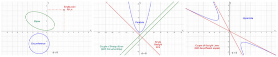
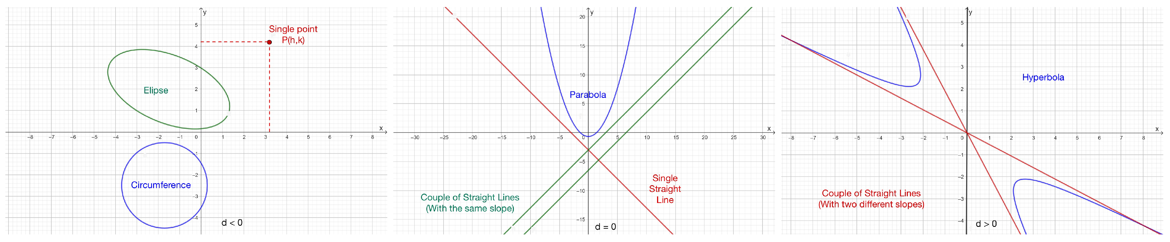
First, it is important to point out that if (1) corresponds to a locus in ${\mathbb{R}}^2$, then it will fall in only one of the following cases: single straight line, circumference (degenerate or not), ellipse (degenerate or not), parabola (degenerate or not), and hyperbola (degenerate or not) (see Chapter 9-Theorem 2 in [2] and Figure 4 below). Now we proceed with the proof.

Figure 4. All the possible cases of real loci in ${\mathbb{R}}^2$ that can be represented by the general conic equation according to the general criterion of the conic discriminant (18).

(i) Observe that, by Proposition 1(iii), $A=C$ and $B=0$ whenever $R=0$. So, there are only two possibilities in this case. Either (1) corresponds to a single straight line whenever $A=C=0$, or (1) represents a circumference (degenerate or not) when $A=C\ne 0$ (see [2] [Chapters 3–4]).

(ii) By part (i), if (1) corresponds to an ellipse (degenerate or not), a parabola (degenerate or not), or a hyperbola (degenerate or not), then $R\ne 0$. Consider the rotation angle of any of these loci to be $\theta \in \left[0,{\displaystyle \frac{\pi }{2}}\right[$. So, (6)–(9), Corollary 1, and Proposition 1(i) imply the following relations: $A^{\prime }=A{cos}^2\theta +Bsin\theta cos\theta +C{sin}^2\theta =A{\displaystyle \frac{A-C+R}{2R}}+B{\displaystyle \frac{B}{2R}}+C{\displaystyle \frac{C-A+R}{2R}}={\displaystyle \frac{(A+C)R+{(A-C)}^2+B^2}{2R}}={\displaystyle \frac{(A+C)R+R^2}{2R}}={\displaystyle \frac{A+C+R}{2}}$, $C^{\prime }=A{sin}^2\theta -Bsin\theta cos\theta +C{cos}^2\theta =A{\displaystyle \frac{C-A+R}{2R}}-B{\displaystyle \frac{B}{2R}}+C{\displaystyle \frac{A-C+R}{2R}}={\displaystyle \frac{(A+C)R-\left[{(A-C)}^2+B^2\right]}{2R}}={\displaystyle \frac{(A+C)R-R^2}{2R}}={\displaystyle \frac{A+C-R}{2}}$, $D^{\prime }=Dcos\theta +Esin\theta =D\sqrt{{\displaystyle \frac{A-C+R}{2R}}}+E\sqrt{{\displaystyle \frac{C-A+R}{2R}}}=\sqrt{{\displaystyle \frac{1}{2}}\left(1+{\displaystyle \frac{A-C}{R}}\right)}+E\sqrt{{\displaystyle \frac{1}{2}}\left(1-{\displaystyle \frac{A-C}{R}}\right)}$ and $E^{\prime }=-Dsin\theta +Ecos\theta =E\sqrt{{\displaystyle \frac{A-C+R}{2R}}}-D\sqrt{{\displaystyle \frac{C-A+R}{2R}}}=E\sqrt{{\displaystyle \frac{1}{2}}\left(1+{\displaystyle \frac{A-C}{R}}\right)}-D\sqrt{{\displaystyle \frac{1}{2}}\left(1-{\displaystyle \frac{A-C}{R}}\right)}$. Finally, the equivalence between (1), (2), and (5) guarantees the invariance of F under rotations. □

Observe that the cases of the single straight line and the circumference (degenerate or not) are the only ones in which (17) is undefined due to $R=0$, while rotations do not have any sense in these cases. In addition, if $\theta =B=0\ne R$, then this is the only case in which Theorem 3(ii) implies that (1) and (2) are identical because this is the only case in which $x=x^{\prime }$ and $y=y^{\prime }$. So, this is the reason why from here onward, we say that a locus that corresponds to (1) is non-rotated whenever $\theta =0$.

Example 5.

Now we look into the practicality of (17). To this end, consider again Examples 1–3. It is clear that $A=43$, $B=-14\sqrt{3}$, $C=57$, $D=-36\sqrt{3}$, $E=36$, and $F=540$ in Example 1, and $R_1=-28$ follows from Example 4. Hence, (17) yields ${\displaystyle \frac{43+57+(-28)}{2}}{\left(x^{\prime }\right)}^2+{\displaystyle \frac{43+57-(-28)}{2}}{\left(y^{\prime }\right)}^2+\left[-36\sqrt{3}\sqrt{{\displaystyle \frac{1}{2}}\left(1+{\displaystyle \frac{43-57}{-28}}\right)}+(-36)\sqrt{{\displaystyle \frac{1}{2}}\left(1-{\displaystyle \frac{43-57}{-28}}\right)}\right]x^{\prime }+\left[-36\sqrt{{\displaystyle \frac{1}{2}}\left(1+{\displaystyle \frac{43-57}{-28}}\right)}-\left(-36\sqrt{3}\right)\sqrt{{\displaystyle \frac{1}{2}}\left(1-{\displaystyle \frac{43-57}{-28}}\right)}\right]y^{\prime }-540=0$, which instantly reduces to $9{\left(x^{\prime }\right)}^2+16{\left(y^{\prime }\right)}^2-18x^{\prime }-135=0.$ Now consider Example 2, so $A=9$, $B=24$, $C=16$, $D=80$, $E=-60$, and $F=0$, whereas $R_2=25$ follows from Example 4. Hence, we use (17) to obtain ${\displaystyle \frac{9+16+25}{2}}{\left(x^{\prime }\right)}^2+{\displaystyle \frac{9+16-25}{2}}{\left(y^{\prime }\right)}^2+\left[80\sqrt{{\displaystyle \frac{1}{2}}\left(1+{\displaystyle \frac{9-16}{25}}\right)}+(-60)\sqrt{{\displaystyle \frac{1}{2}}\left(1-{\displaystyle \frac{9-16}{25}}\right)}\right]x^{\prime }+\left[-60\sqrt{{\displaystyle \frac{1}{2}}\left(1+{\displaystyle \frac{9-16}{25}}\right)}-80\sqrt{{\displaystyle \frac{1}{2}}\left(1-{\displaystyle \frac{9-16}{25}}\right)}\right]y^{\prime }=0$, which instantly reduces to ${\left(x^{\prime }\right)}^2-4y^{\prime }=0.$ Finally, consider Example 3; then, $A=C=D=E=0$ and $F=-1$, whereas $R_3=1$ follows from Example 4; hence, (17) yields ${\displaystyle \frac{0+0+1}{2}}{\left(x^{\prime }\right)}^2+{\displaystyle \frac{0+0-1}{2}}{\left(y^{\prime }\right)}^2+\left[0\sqrt{{\displaystyle \frac{1}{2}}\left(1+{\displaystyle \frac{0+0}{1}}\right)}+0\sqrt{{\displaystyle \frac{1}{2}}\left(1-{\displaystyle \frac{0-0}{1}}\right)}\right]x^{\prime }+\left[0\sqrt{{\displaystyle \frac{1}{2}}\left(1+{\displaystyle \frac{0+0}{1}}\right)}-0\sqrt{{\displaystyle \frac{1}{2}}\left(1-{\displaystyle \frac{0-0}{1}}\right)}\right]y^{\prime }-1=0$, which reduces to ${\displaystyle \frac{{\left(x^{\prime }\right)}^2}{2}}-{\displaystyle \frac{{\left(y^{\prime }\right)}^2}{2}}=1.$

Example 5 illustrates how (17) solves the classical problem of transforming (1) into (2) faster than any other previously known method for solving this problem.

4. Illustrations

4.1. Two Well-Known Results

We now show how two previously known results become immediate consequences of Theorem 3.

Corollary 2

(Invariants under Rotations). Let $A,B,C,D,E,F,A^{\prime },C^{\prime },D^{\prime },E^{\prime }\in \mathbb{R}$ be such that (1)–(2) correspond to the same locus on the Cartesian plane, as in Theorem 3(ii). Then,

(i)  $A^{\prime }+C^{\prime }=A+C$,

(ii)  ${\left(D^{\prime }\right)}^2+{\left(E^{\prime }\right)}^2=D^2+E^2$,

(iii)  $-4A^{\prime }{C}^{\prime }=B^2-4AC$,

(iv)  $\left|A^{\prime }-C^{\prime }\right|=\sqrt{{(A-C)}^2+B^2}$.

Proof. 

The direct substitution of the coefficients $A^{\prime },C^{\prime },D^{\prime },E^{\prime }\in \mathbb{R}$, given by Theorem 3(ii), into the left-hand sides of (i)–(iv) yields the respective right-hand sides. For instance, by the first two coefficients of (17), we have $A^{\prime }+C^{\prime }={\displaystyle \frac{A+C+R}{2}}+{\displaystyle \frac{A+C-R}{2}}=A+C$, which proves (i). The remainder of these equalities are proved analogously. □

Corollary 3

(The General Criterion of the Conic Discriminant). Let $A,B,C,D,E,F\in \mathbb{R}$ be such that (1) corresponds to a locus in ${\mathbb{R}}^2$, and define the conic discriminant as

$$d:=B^2-4AC.$$

(18)

Then,

(i) $d<0$ if and only if the locus in question is an ellipse, a circumference, or a single point. See the leftmost subfigure in Figure 4.

(ii) $d=0$ if and only if the locus in question is a parabola, a single straight line, or a couple of straight lines with the same slope. See the center subfigure in Figure 4.

(iii) $d>0$ if and only if the locus in question is a hyperbola or a couple of straight lines with different slopes. See the rightmost subfigure in Figure 4.

Proof. 

Case 1. Suppose that $R=0$. Then, Theorem 3(i) shows that (1) represents a single straight line or a circumference (degenerate or not). So, plugging $A=B=C=0$ into (18) yields $d=0$ for the straight line. The substitution of $A=C\ne 0=B$ into (18) results in $d=-4A^2<0$ for the circumference and its degenerate case, which corresponds to the single point on the Cartesian plane $(h,k)$, whose canonical equation is ${(x-h)}^2+{(y-k)}^2=0$.

Case 2. Suppose that $R\ne 0$, then Theorem 3(ii) ensures that (1) corresponds to an ellipse (degenerate or not), to a parabola (degenerate or not), or a hyperbola (degenerate or not). In addition, note that Corollary 2(iii) guarantees $d=B^2-4AC=-4A^{\prime }{C}^{\prime }$. Now consider the following three possibilities for d.

(i) $d<0$ is equivalent to $A^{\prime }{C}^{\prime }>0$, which, at the same time is a necessary and sufficient condition so that $A^{\prime }\ne C^{\prime }$ with $\mathrm{sgn}\left(A^{\prime }\right)=\mathrm{sgn}\left(C^{\prime }\right)\ne 0$. The latter occurs whenever (1)–(2) correspond to an ellipse (or to its degenerate case: the single point $(h^{\prime },k^{\prime })$ on the Cartesian plane generated by some rotation angle $\theta \in \left[0,{\displaystyle \frac{\pi }{2}}\right[$ characterized by ${\displaystyle \frac{{(x^{\prime }-h^{\prime })}^2}{a^2}}+{\displaystyle \frac{{(y^{\prime }-k^{\prime })}^2}{b^2}}=0$, with $a>0$, $b>0$, and $a\ne b$).

(ii) $d=0$ is equivalent to $A^{\prime }{C}^{\prime }=0$, which, at the same time, is a necessary and sufficient condition so that there are two options:

Option 1. If $A^{\prime }\ne 0=C^{\prime }$, then (1)–(2) correspond to a parabola whose focal axis is parallel to the $y^{\prime }$-axis generated by some rotation angle $\theta \in \left[0,{\displaystyle \frac{\pi }{2}}\right[$ or to the degenerate case where $E^{\prime }=0$ and ${\left(D^{\prime }\right)}^2-4A^{\prime }F\ge 0$. This degenerate case corresponds to two straight lines parallel to the $y^{\prime }$-axis. (Note that if ${\left(D^{\prime }\right)}^2-4A^{\prime }F>0$, then these lines will be different from each other. If it turns out that ${\left(D^{\prime }\right)}^2-4A^{\prime }F=0$, then the lines are the same. Finally, observe that the case ${\left(D^{\prime }\right)}^2-4A^{\prime }F<0$ is unacceptable because it corresponds to an imaginary locus.)

Option 2. If $A^{\prime }=0\ne C^{\prime }$, then (1)–(2) correspond to a parabola whose focal axis is parallel to the $x^{\prime }$-axis generated by some rotation angle $\theta \in \left[0,{\displaystyle \frac{\pi }{2}}\right[$ or to the degenerate case where $D^{\prime }=0$ and ${\left(E^{\prime }\right)}^2-4C^{\prime }F\ge 0$. This degenerate case corresponds to two straight lines parallel to the $x^{\prime }$-axis. (Note that if ${\left(E^{\prime }\right)}^2-4C^{\prime }F>0$, then these lines will be different from each other. If it turns out that ${\left(E^{\prime }\right)}^2-4C^{\prime }F=0$, then the lines are the same. Finally, observe that the case ${\left(D^{\prime }\right)}^2-4A^{\prime }F<0$ is unacceptable because it corresponds to an imaginary locus.)

(iii) $d>0$ is equivalent to $A^{\prime }{C}^{\prime }<0$, which, at the same time is a necessary and sufficient condition so that $\mathrm{sgn}\left(A^{\prime }\right)=-\mathrm{sgn}\left(C^{\prime }\right)\ne 0$. The latter occurs when (1)–(2) correspond to a hyperbola or its degenerate case: a pair of straight lines whose respective slopes are different from each other and at most one of them is undefined. Otherwise, (1)–(2) would correspond to item (ii) just above. Additionally, this degenerate case occurs when (2) can be written as $A^{\prime }{(x^{\prime }-h^{\prime })}^2+C^{\prime }{(y^{\prime }-k^{\prime })}^2=0$, where $(h^{\prime },k^{\prime })$ are the coordinates of the intersection of such lines on the Cartesian plane generated by some rotation angle $\theta \in \left[0,{\displaystyle \frac{\pi }{2}}\right[$. □

The typical proofs of Corollaries 2 and 3 are based on the application of trigonometric identities over the coefficients of (5). However, this argumentation inexorably depends on the rotation angle $\theta$ (see pp. 100–102, and 105–106 in [12]). Our proofs show how these well-known results can be seen as consequences of Theorem 3, featuring only algebraic manipulations without using trigonometric functions. On the other hand, note that the general criterion of the conic discriminant defined in (18) is not applied in Examples 1–3; nevertheless, when the criterion is applied to these examples, one obtains $d_1={(-14\sqrt{3})}^2-4\left(43\right)\left(57\right)=-9216<0$, $d_2={\left(24\right)}^2-4\left(9\right)\left(16\right)=0,$ and $d_3=1^2-4\left(0\right)\left(0\right)=1>0.$ These results are consistent with respect to what Figure 1, Figure 2 and Figure 3 show.

4.2. What About Degenerate Cases?

We now explore the degenerate cases of conic sections by applying Theorem 3.

Example 6.

Consider the equations

$$\begin{array}{ccc}\hfill x^2+y^2+8x+16y+80& =& 0,\hfill \end{array}$$

(19)

$$\begin{array}{ccc}\hfill 29x^2-24xy+36y^2+40x+480y+2000& =& 0,\hfill \end{array}$$

(20)

and the point $P(-4,-8)$. It is clear that the coordinates of P meet both equations. So, P might be an intersection point between the two loci represented by (19) and (20). However, (19) corresponds to a degenerate circumference due to the fact that its canonical form is ${(x+4)}^2+{(y+8)}^2=0$; therefore, P is the unique point in ${\mathbb{R}}^2$ whose coordinates satisfy (19). Meanwhile, if Theorem 3 is applied to (20), then one obtains $R=\mathrm{sgn}(-24)\sqrt{{(29-36)}^2+{(-24)}^2}=-25.$ Thus, ${\displaystyle \frac{29+36+(-25)}{2}}{\left(x^{\prime }\right)}^2+{\displaystyle \frac{29+36-(-25)}{2}}{\left(y^{\prime }\right)}^2+\left[40\sqrt{{\displaystyle \frac{1}{2}}\left(1+{\displaystyle \frac{29-36}{-25}}\right)}+480\sqrt{{\displaystyle \frac{1}{2}}\left(1-{\displaystyle \frac{29-36}{-25}}\right)}\right]x^{\prime }+\left[480\sqrt{{\displaystyle \frac{1}{2}}\left(1+{\displaystyle \frac{29-36}{-25}}\right)}-40\sqrt{{\displaystyle \frac{1}{2}}\left(1-{\displaystyle \frac{29-36}{-25}}\right)}\right]y^{\prime }+2000=0$; so, this is reduced to

$$4{\left(x^{\prime }\right)}^2+9{\left(y^{\prime }\right)}^2+64x^{\prime }+72y^{\prime }+400=0,$$

(21)

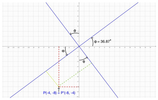
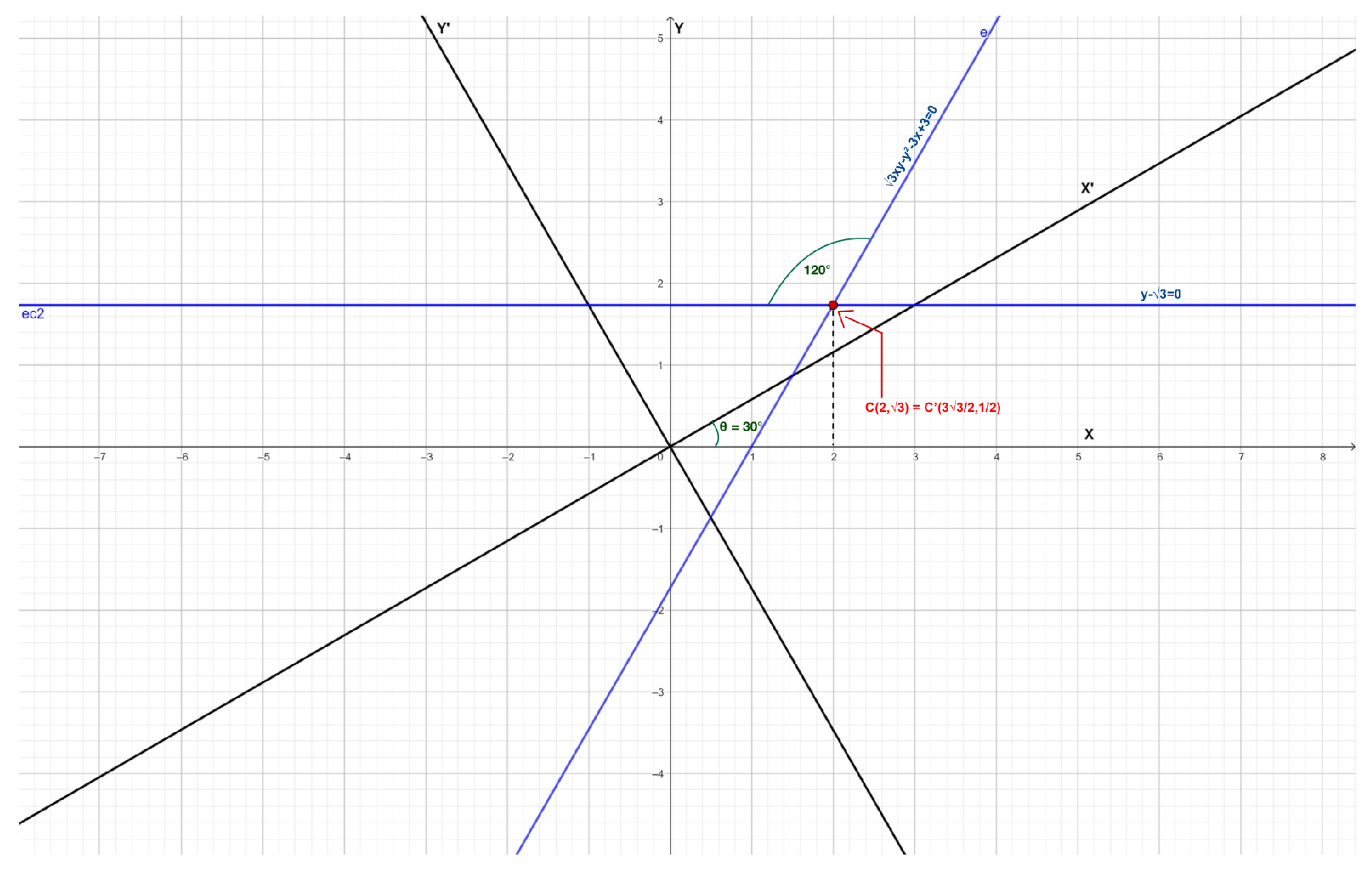
which seems to be the general equation of a non-rotated ellipse. Actually, Corollary 3 enables us to verify this, since $d=-3600<0$ in (20). However, (21) can be rewritten as $4{(x^{\prime }+8)}^2+9{(y^{\prime }+4)}^2=0$; so, it is impossible that it represents a non-degenerate ellipse. In fact, it corresponds to a degenerate ellipse, whereas $P^{\prime }(-8,-4)$ is the only point in the whole rotated Cartesian plane whose coordinates satisfy this equation. So, to know the coordinates of $P^{\prime }$ in the non-rotated Cartesian plane, it is necessary to apply the transformations (3)–(4) to these coordinates, considering that Corollaries 1(i) and (ii) imply $sin\theta ={\displaystyle \frac{3}{5}}$ and $cos\theta ={\displaystyle \frac{4}{5}}$. So, $x=x^{\prime }cos\theta -y^{\prime }sin\theta =-8{\displaystyle \frac{4}{5}}-(-4){\displaystyle \frac{3}{5}}=-4$, and $y=x^{\prime }sin\theta +y^{\prime }cos\theta =-8{\displaystyle \frac{3}{5}}+(-4){\displaystyle \frac{4}{5}}=-8$, which proves that P and $P^{\prime }$ are the same points, despite each one being located in two systems of rectangular coordinates whose only difference is a rotation of the Cartesian axes generated by the angle $\theta \approx 36.{87}^{\circ }$ (see Figure 5).

Figure 5. Coordinates of P and $P^{\prime }$ in both Cartesian planes (the non-rotated one and the one rotated by $\theta$).

Finally, although (19) and (20) are two different equations, they correspond to the same locus, which is a single point that is simultaneously a degenerate case of the circumference and a degenerate case of the ellipse. In fact, it can be proven that for each single point in ${\mathbb{R}}^2$, there is an infinite family of equations of degenerate ellipses that represent it. And at the same time, there is only one equation of a degenerate circumference that represents it.

Example 7.

Let $a,b,c\in \mathbb{R}$ be such that $a\ne 0\ne b$, and consider the locus characterized by $ax+by+c=0$, which corresponds to a single straight line on the Cartesian plane, whose slope is $m=tan\alpha =-{\displaystyle \frac{a}{b}}\ne 0$, where α stands for its angle of inclination. Note that this straight line is not parallel to any of the two Cartesian axes (see p. 68 in [2]). So,

$$0^2={(ax+by+c)}^2=a^2{x}^2+2abxy+b^2{y}^2+2acx+2bcy+c^2=0.$$

(22)

Therefore, the coefficients of (1) in this case are $A=a^2$, $B=2ab\ne 0$, $C=b^2$, $D=2ac$, $E=2bc$, and $F=c^2$, and $d={\left(2ab\right)}^2-4a^2{b}^2=0$. Then, it is clear that the law of signs and (10) yield $\mathrm{sgn}\left(B\right)=\mathrm{sgn}\left(2ab\right)=-\mathrm{sgn}\left(m\right)\ne 0$. Thus, $R=\mathrm{sgn}\left(2ab\right)\sqrt{{\left(a^2-b^2\right)}^2+{\left(2ab\right)}^2}=-\mathrm{sgn}\left(m\right)\left(a^2+b^2\right)\ne 0$ due to $a\ne 0\ne b$ guarantees $a^2+b^2>0$. Now, consider the only two possible cases as follows:

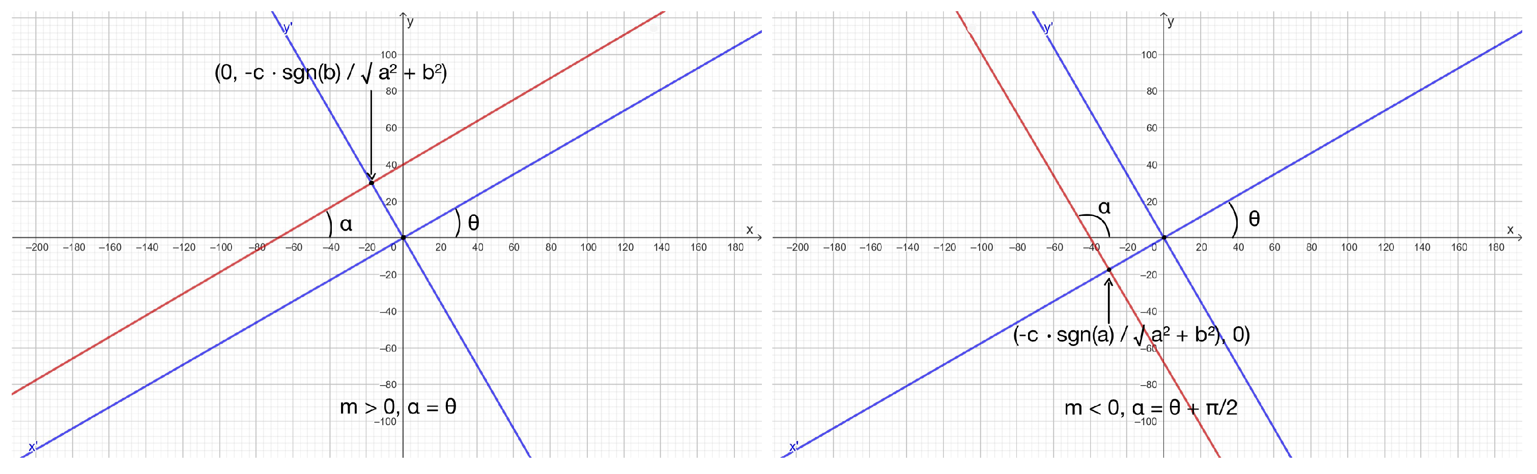
Case 1.  If $m>0$, then $R=-\left(a^2+b^2\right)<0$. Theorem 3(ii) yields the following: ${\displaystyle \frac{a^2+b^2-\left(a^2+b^2\right)}{2}}{\left(x^{\prime }\right)}^2+{\displaystyle \frac{a^2+b^2+\left(a^2+b^2\right)}{2}}{\left(y^{\prime }\right)}^2+\left[2ac\sqrt{{\displaystyle \frac{1}{2}}\left(1-{\displaystyle \frac{a^2-b^2}{a^2+b^2}}\right)}+2bc\sqrt{{\displaystyle \frac{1}{2}}\left(1+{\displaystyle \frac{a^2-b^2}{a^2+b^2}}\right)}\right]x^{\prime }+\left[2bc\sqrt{{\displaystyle \frac{1}{2}}\left(1-{\displaystyle \frac{a^2-b^2}{a^2+b^2}}\right)}+2ac\sqrt{{\displaystyle \frac{1}{2}}\left(1+{\displaystyle \frac{a^2-b^2}{a^2+b^2}}\right)}\right]y^{\prime }+c^2=0$, which reduces to $\left(a^2+b^2\right){\left(y^{\prime }\right)}^2+2{\displaystyle \frac{a\left|b\right|+\left|a\right|b}{\sqrt{a^2+b^2}}}c{x}^{\prime }+2{\displaystyle \frac{b\left|b\right|+\left|a\right|a}{\sqrt{a^2+b^2}}}c{y}^{\prime }+c^2=0.$ Now note that since $m>0$, then $\mathrm{sgn}\left(a\right)=-\mathrm{sgn}\left(b\right)\ne 0$, so Property 2 implies $a\left|b\right|+\left|a\right|b=a\left[b\mathrm{sgn}\right(b\left)\right]+\left[a\mathrm{sgn}\right(a\left)\right]b=ab\left[\mathrm{sgn}\right(a)+\mathrm{sgn}(b\left)\right]=0$ and $b\left|b\right|-\left|a\right|a=\mathrm{sgn}\left(b\right)b^2-\mathrm{sgn}\left(a\right)a^2=\mathrm{sgn}\left(b\right)\left(a^2+b^2\right).$ Hence, (22) reduces to $0=\left(a^2+b^2\right){\left(y^{\prime }\right)}^2+2c\sqrt{a^2+b^2}\mathrm{sgn}\left(b\right)y^{\prime }+c^2={\left[\sqrt{a^2+b^2}{y}^{\prime }+c·\mathrm{sgn}\left(b\right)\right]}^2,$ where the last equality holds by Property 3. Therefore, (22) also corresponds to a couple of parallel straight lines with the same slope and the same y-intercept. In fact, these straight lines are also parallel to the rotated $x^{\prime }$-axis and intersect the rotated $y^{\prime }$-axis at the point whose coordinates on the rotated Cartesian plane are given by the pair $\left(0,-{\displaystyle \frac{c\mathrm{sgn}\left(b\right)}{\sqrt{a^2+b^2}}}\right)$. In addition, Theorem 2 implies that $tan\theta ={\displaystyle \frac{b^2-a^2-\left(a^2+b^2\right)}{2ab}}=-{\displaystyle \frac{a}{b}}=m=tan\alpha >0.$ Thus, $\alpha \in \left]0,{\displaystyle \frac{\pi }{2}}\right[$ and $\alpha =\theta$.

Case 2.  If $m<0$, then $R=a^2+b^2>0$ and Theorem 3(ii) yields the following: ${\displaystyle \frac{a^2+b^2+a^2+b^2}{2}}{\left(x^{\prime }\right)}^2+{\displaystyle \frac{a^2+b^2-\left(a^2+b^2\right)}{2}}{\left(y^{\prime }\right)}^2+\left[2ac\sqrt{{\displaystyle \frac{1}{2}}\left(1+{\displaystyle \frac{a^2-b^2}{a^2+b^2}}\right)}+2bc\sqrt{{\displaystyle \frac{1}{2}}\left(1-{\displaystyle \frac{a^2-b^2}{a^2+b^2}}\right)}\right]x^{\prime }+\left[2bc\sqrt{{\displaystyle \frac{1}{2}}\left(1+{\displaystyle \frac{a^2-b^2}{a^2+b^2}}\right)}+2ac\sqrt{{\displaystyle \frac{1}{2}}\left(1-{\displaystyle \frac{a^2-b^2}{a^2+b^2}}\right)}\right]y^{\prime }+c^2=0$. Note that this expression can be reduced to $\left(a^2+b^2\right){\left(x^{\prime }\right)}^2+{\displaystyle \frac{2\left(a\right|a|+b|b\left|\right)c}{\sqrt{a^2+b^2}}}{x}^{\prime }+{\displaystyle \frac{2\left(\right|a|b-a|b\left|\right)c}{\sqrt{a^2+b^2}}}{y}^{\prime }+c^2=0.$ Now, since $m<0$, then $\mathrm{sgn}\left(a\right)=\mathrm{sgn}\left(b\right)\ne 0$. Then, Property 2 implies that $a\left|a\right|+b\left|b\right|=\mathrm{sgn}\left(a\right)a^2+\mathrm{sgn}\left(b\right)b^2=\mathrm{sgn}\left(a\right)\left(a^2+b^2\right)$ and $\left|a\right|b-a\left|b\right|=ab\left[\mathrm{sgn}\left(a\right)-\mathrm{sgn}\left(b\right)\right]=0.$ Hence, (22) reduces to $0=\left(a^2+b^2\right){\left(x^{\prime }\right)}^2+2c·\mathrm{sgn}\left(a\right)\sqrt{a^2+b^2}{x}^{\prime }+c^2={\left[\sqrt{a^2+b^2}{x}^{\prime }+c·\mathrm{sgn}\left(a\right)\right]}^2,$ where the last equality holds by Property 3. Therefore, (22) also corresponds to a couple of parallel straight lines with the same slope and the same y-intercept. These lines are also parallel to the rotated $y^{\prime }$-axis and intersect the rotated $x^{\prime }$-axis in the point whose coordinates on the rotated Cartesian plane are given by the pair $\left(-{\displaystyle \frac{c\mathrm{sgn}\left(a\right)}{\sqrt{a^2+b^2}}},0\right)$. In addition, Theorem 2 implies that $tan\theta ={\displaystyle \frac{b^2-a^2+a^2+b^2}{2ab}}={\displaystyle \frac{b}{a}}=-{\displaystyle \frac{1}{m}}=-{\displaystyle \frac{1}{tan\alpha }}>0.$ Thus, $\alpha \in \left]{\displaystyle \frac{\pi }{2}},\pi \right[$ and $\alpha =\theta +{\displaystyle \frac{\pi }{2}}$.

Observe that, in both cases, the shortest distance between the origin and the straight line (22) is always ${\displaystyle \frac{\left|c\right|}{\sqrt{a^2+b^2}}}$. Therefore, if Theorem 3 is applied to a couple of straight lines with the same slope that are not parallel to any of the Cartesian axes x and y but have the same y-axis intersection, then the corresponding equation also corresponds to a couple of straight lines with the same y-axis intersection, but this time, they are parallel to only one of the rotated axes $x^{\prime }$ and $y^{\prime }$ generated by the rotation angle $\theta \in \left]0,{\displaystyle \frac{\pi }{2}}\right[$. Note that this angle coincides with the angle of inclination of the straight lines in question with respect to the Cartesian plane whose axes are x and y, or it coincides with the angle of inclination of all the straight lines that are orthogonal to (22). Thus, Cases 1 and 2 occur depending on the sign of the slope of (22). Figure 6 illustrates the cases presented here.

Figure 6. Plots of the two possible cases in Example 7 (Case 1 on the left and Case 2 on the right).

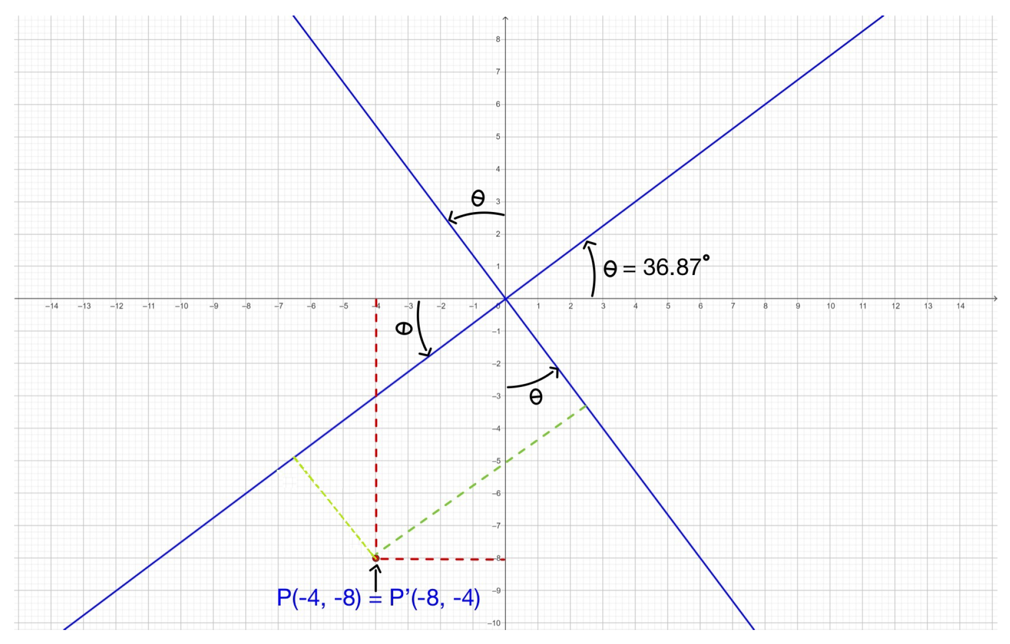
Example 8.

Consider the locus characterized by

$$\sqrt{3}xy-y^2-3x+3=0.$$

(23)

Then, $A=E=0,B=\sqrt{3},C=-1,D=-3,F=3$ and $d={\sqrt{3}}^2-4\left(0\right)(-1)=3>0$. So, Corollary 3 implies that (23) corresponds to a hyperbola or a couple of straight lines with different slopes. On the other hand, the conic radical is $R=\mathrm{sgn}\left(\sqrt{3}\right)\sqrt{{(0+1)}^2+{\left(\sqrt{3}\right)}^2}=2$, so Theorem 3(ii) yields the following: ${\displaystyle \frac{0-1+2}{2}}{\left(x^{\prime }\right)}^2+{\displaystyle \frac{0-1-2}{2}}{\left(y^{\prime }\right)}^2+\left[-3\sqrt{{\displaystyle \frac{1}{2}}\left(1+{\displaystyle \frac{0+1}{2}}\right)}+0\sqrt{{\displaystyle \frac{1}{2}}\left(1-{\displaystyle \frac{0+1}{2}}\right)}\right]x^{\prime }+\left[0\sqrt{{\displaystyle \frac{1}{2}}\left(1+{\displaystyle \frac{0+1}{2}}\right)}-(-3)\sqrt{{\displaystyle \frac{1}{2}}\left(1-{\displaystyle \frac{0+1}{2}}\right)}\right]y^{\prime }+3=0$, which reduces to ${\displaystyle \frac{1}{2}}{\left(x^{\prime }\right)}^2-{\displaystyle \frac{3}{2}}{\left(y^{\prime }\right)}^2-{\displaystyle \frac{3\sqrt{3}}{2}}{x}^{\prime }+{\displaystyle \frac{3}{2}}{y}^{\prime }+3=0.$

In other words, (23) appears to be the general equation of a rotated hyperbola. However, the expression above can be rewritten as ${\left(x^{\prime }-{\displaystyle \frac{3\sqrt{3}}{2}}\right)}^2-{\left(y^{\prime }-{\displaystyle \frac{1}{2}}\right)}^2=0,$ which cannot correspond to a hyperbola. Hence, (23) corresponds to a couple of straight lines with different slopes, and the coordinates of their intersection point on the rotated Cartesian axes are $C^{\prime }\left({\displaystyle \frac{3\sqrt{3}}{2}},{\displaystyle \frac{1}{2}}\right)$. The general equations of these straight lines are

$$\begin{array}{ccc}\hfill x^{\prime }-\sqrt{3}{y}^{\prime }-\sqrt{3}& =& 0,\hfill \end{array}$$

(24)

$$\begin{array}{ccc}\hfill x^{\prime }+\sqrt{3}{y}^{\prime }-2\sqrt{3}& =& 0,\hfill \end{array}$$

(25)

respectively. It is straightforward to see that the slopes are $m_1^{\prime }={\displaystyle \frac{1}{\sqrt{3}}}$ and $m_2^{\prime }=-{\displaystyle \frac{1}{\sqrt{3}}}$ (note that $m_1^{\prime }=-m_2^{\prime }\ne 0$). Therefore, the angle between these straight lines is ${\beta }^{\prime }={\alpha }_2^{\prime }-{\alpha }_1^{\prime }={120}^{\circ }$. Now, Theorems 1 and 2 imply that the rotation angle in question is $\theta ={30}^{\circ }$ and (23) can be rewritten as $\left(\sqrt{3}x-y-\sqrt{3}\right)\left(y-\sqrt{3}\right)=0$. Then,

$$\begin{array}{ccc}\hfill \sqrt{3}x-y-\sqrt{3}& =& 0,\hfill \end{array}$$

(26)

$$\begin{array}{ccc}\hfill y-\sqrt{3}& =& 0\hfill \end{array}$$

(27)

correspond to the general equations of two different non-parallel straight lines, and the coordinates of their intersection point on the non-rotated Cartesian axes are $C(2,\sqrt{3})$; their respective slopes are $m_1=\sqrt{3}$ and $m_2=0$ (note that $|m_1|\ne |m_2|$). Their respective inclination angles are ${\alpha }_1={60}^{\circ }$ and ${\alpha }_2=0^{\circ }$ (or ${180}^{\circ }$). In addition, the angle between these straight lines is $\beta =arctan\left({\displaystyle \frac{m_2-m_1}{1+m_1{m}_2}}\right)=arctan\left({\displaystyle \frac{0-\sqrt{3}}{1+0\sqrt{3}}}\right)=arctan(-\sqrt{3})={120}^{\circ }$ (see p. 2 in [1]). An application of the inverse transformations defined by (3) and (4) to point C gives us the coordinates on the rotated Cartesian axes (see pp. 53–54 in [13]): $x^{\prime }=2cos\left({30}^{\circ }\right)+\sqrt{3}sin\left({30}^{\circ }\right)={\displaystyle \frac{3\sqrt{3}}{2}}$ and $y^{\prime }=-2sin\left({30}^{\circ }\right)+\sqrt{3}cos\left({30}^{\circ }\right)={\displaystyle \frac{1}{2}}.$ So, we conclude that C and $C^{\prime }$ are representations in different Cartesian systems of the same point (one of them is a rotation of the other of $\theta ={30}^{\circ }$). Recall from Example 6 that this is the same situation experienced by points P and $P^{\prime }$. Therefore, if the inverse transformations of (3)–(4) are applied to (24)–(25), then we obtain the following: $x^{\prime }-\sqrt{3}{y}^{\prime }-\sqrt{3}=xcos\left({30}^{\circ }\right)+ysin\left({30}^{\circ }\right)-\sqrt{3}(-xsin\left({30}^{\circ }\right)+ycos\left({30}^{\circ }\right)-\sqrt{3}=\sqrt{3}x-y-\sqrt{3}=0$, and $x^{\prime }+\sqrt{3}{y}^{\prime }-2\sqrt{3}=xcos\left({30}^{\circ }\right)+ysin\left({30}^{\circ }\right)+\sqrt{3}(-xsin\left({30}^{\circ }\right)+ycos\left({30}^{\circ }\right))-2\sqrt{3}=2(y-\sqrt{3})=0$, which is equivalent to $y-\sqrt{3}=0$. We conclude that, in the same sense that C and $C^{\prime }$ are equivalent to each other, we can also say that (26) and (27) are equivalent to (24) and (25), respectively. Moreover, $\beta ={\beta }^{\prime }$ and if the rotation angle θ is subtracted from ${\alpha }_1$ and ${\alpha }_2$, then we obtain ${\alpha }_1^{\prime }$ and ${\alpha }_2^{\prime }$, respectively (Figure 7 illustrates the plots of this example).

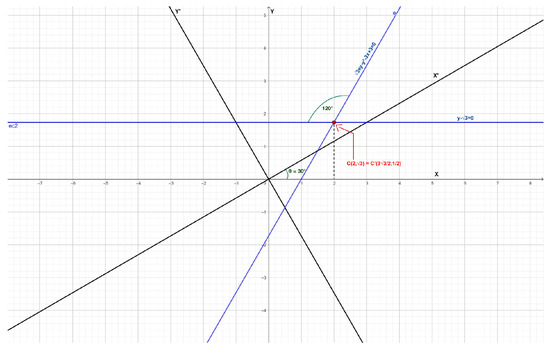
Figure 7. Plots of the locus described by (23) in both Cartesian planes (the non-rotated one and the one rotated by $\theta ={30}^{\circ }$).

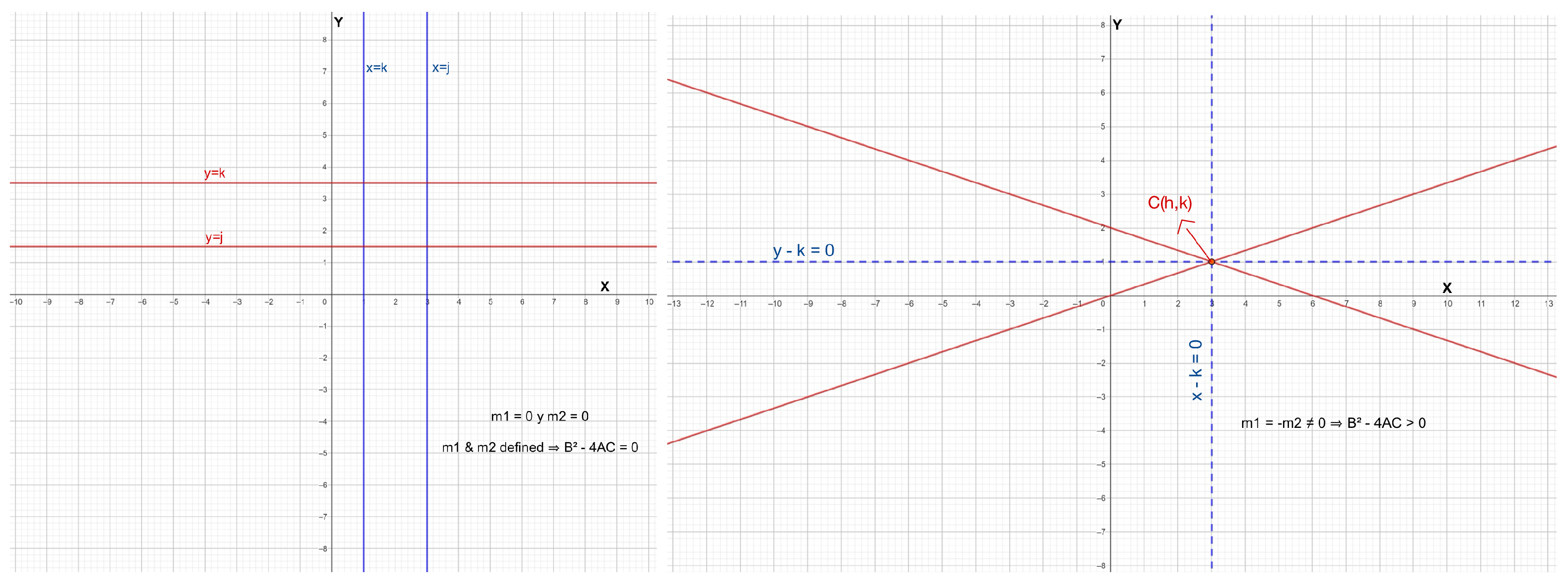
The analytic method from Example 7 can be used to prove that if (1) represents two straight lines with slopes $m_1$ and $m_2$ such that $|m_1|\ne |m_2|$, the rotation angle from Theorems 1 and 2 results in a rotated Cartesian plane, where the new slopes $m_1^{\prime }$ and $m_2^{\prime }$ satisfy $m_1^{\prime }=-m_2^{\prime }\ne 0$. Theorem 3(ii) provides a new equation for these lines in the rotated plane. Example 8 is just a particular case of this. For cases where $m_1=-m_2$ or both slopes are undefined, the following occurs (see Figure 8):

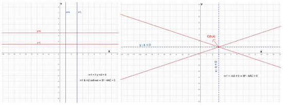
Figure 8. Cases $m_1=-m_2=0$ or both slopes undefined (left), and $m_1=-m_2\ne 0$ (right).

• If $m_1=-m_2=0$ or both slopes are undefined, the lines are parallel to one Cartesian axis and $d=0$.
• If $m_1=-m_2\ne 0$, the lines intersect at $C(h,k)$, and the plot is symmetric with respect to $x-h=0$ and $y-k=0$, with $d>0$. These lines are the asymptotes of two infinite families of concentric hyperbolas centered at $C(h,k)$, with one family having a vertical focal axis and the other having a horizontal focal axis.

4.3. Some Curious Cases

Example 9.

Let

$${\left(x^{\prime }\right)}^2-1=0.$$

(28)

It is well-known that the corresponding locus is the pair of mutually parallel straight lines $x^{\prime }+1=0$ and $x^{\prime }-1=0$. Now consider the angles ${\theta }_1={\displaystyle \frac{\pi }{6}}$ and ${\theta }_2={\displaystyle \frac{2\pi }{3}}$. Thus, $sin{\theta }_1={\displaystyle \frac{1}{2}}$, $cos{\theta }_1=sin{\theta }_2={\displaystyle \frac{\sqrt{3}}{2}}$, and $cos{\theta }_2=-{\displaystyle \frac{1}{2}}$. Plugging (3) and (4) into (28) yields

$$\begin{array}{ccc}\hfill {\left(x^{\prime }\right)}^2-1& =& {(xcos{\theta }_1+ysin{\theta }_1)}^2-1={\left({\displaystyle \frac{\sqrt{3}}{2}}x+{\displaystyle \frac{1}{2}}y\right)}^2-1={\displaystyle \frac{3}{4}}{x}^2+{\displaystyle \frac{\sqrt{3}}{2}}xy+{\displaystyle \frac{1}{4}}{y}^2-1=0.\hfill \end{array}$$

(29)

So, in this case, $A={\displaystyle \frac{3}{4}}$, $B={\displaystyle \frac{\sqrt{3}}{2}}$, $C={\displaystyle \frac{1}{4}}$, $D=E=0$, and $F=-1$ (note that $d=0$). Hence, $R=1$. The application of (17) to (29) returns us to (28), while Theorems 1 and 2 imply $\theta ={\displaystyle \frac{1}{2}}arctan{\displaystyle \frac{\frac{\sqrt{3}}{2}}{\frac{3}{4}-\frac{1}{4}}}=arctan{\displaystyle \frac{\frac{1}{4}-\frac{3}{4}+1}{\frac{3}{2}}}={\displaystyle \frac{\pi }{6}}={\theta }_1.$ Therefore, the results obtained by Theorems 1–3 are not unexpected because (17) works as an inverse transformation of (3)–(4). On the other hand, if (3)–(4) are applied to (28) with ${\theta }_2$, then

$$\begin{array}{ccc}\hfill {\left(x^{\prime }\right)}^2-1& =& {(xcos{\theta }_2+ysin{\theta }_2)}^2-1={\left(-{\displaystyle \frac{1}{2}}x+{\displaystyle \frac{\sqrt{3}}{2}}y\right)}^2-1={\displaystyle \frac{1}{4}}{x}^2-{\displaystyle \frac{\sqrt{3}}{2}}xy+{\displaystyle \frac{3}{2}}{y}^2-1=0.\hfill \end{array}$$

(30)

So, $A={\displaystyle \frac{1}{4}}$, $B=-{\displaystyle \frac{\sqrt{3}}{2}}$, $C={\displaystyle \frac{3}{4}}$, $D=E=0$, and $F=-1$ (note that in this case, $d=0$ as well). Thus, $R=-1$. The application of (17) to (30) yields

$${\left(y^{\prime }\right)}^2-1=0,$$

(31)

while Theorems 1 and 2 imply $\theta ={\displaystyle \frac{1}{2}}arctan{\displaystyle \frac{-\frac{\sqrt{3}}{2}}{\frac{1}{4}-\frac{3}{4}}}=arctan{\displaystyle \frac{\frac{3}{4}-\frac{1}{4}-1}{-\frac{\sqrt{3}}{2}}}={\displaystyle \frac{\pi }{6}}\ne {\theta }_2.$

Apparently, we have found a counterexample for Theorems 1–2 because the rotation angle ${\theta }_2\notin \left]0,{\displaystyle \frac{\pi }{2}}\right[$. Also, it turns out that (17) is not an inverse transformation of (3)–(4), as the hypotheses of Theorem 3 are not met. However, all of these facts do not pose a contradiction to Theorems 1–3 because their sets of assumptions specifically request that the rotation angle belongs to $\left]0,{\displaystyle \frac{\pi }{2}}\right[$. This means that if one intends to apply these results to loci whose rotation angles are not in this interval, then it will become necessary to subtract a multiple of ${\displaystyle \frac{\pi }{2}}$ beforehand. This is indeed the case of Example 9, as ${\theta }_2={\displaystyle \frac{\pi }{2}}+{\displaystyle \frac{\pi }{6}}$. Therefore, Theorems 1–3 cannot consider (30) as a rotation of (28) with $\theta ={\theta }_2={\displaystyle \frac{2\pi }{3}}$, while they do treat (30) as a rotation of (31) with $\theta ={\theta }_1={\displaystyle \frac{\pi }{6}}$.

Remark 1.

Note that Example 9 shows how a single locus can also be seen as a result of at least two different rotations generated by two different angles. That is, a unique rotated locus is not necessarily generated by one rotation angle θ. In fact, there is an infinite number of rotation angles ${\theta }_k$ that generate it, and their general form is ${\theta }_k=\theta +k{\displaystyle \frac{\pi }{2}}$ for $k=0,\pm 1,\pm 2\dots$ and $\theta \in \left]0,{\displaystyle \frac{\pi }{2}}\right[$. The latter is the only rotation angle considered by Theorems 1–3. In these terms, ${\theta }_0=\theta$.

Example 10.

Consider the well-known case of ${\left(x^{\prime }\right)}^2+1=0$, in which $x^{\prime }=\pm \sqrt{-1}\notin \mathbb{R}$, so this does not correspond to any real locus. Nevertheless, if we take the angle $\theta ={\displaystyle \frac{\pi }{4}}$, then (3)–(4) yield

$$\begin{array}{ccc}\hfill {\left(x^{\prime }\right)}^2+1& =& {\left(xcos{\displaystyle \frac{\pi }{4}}+ysin{\displaystyle \frac{\pi }{4}}\right)}^2+1={\left({\displaystyle \frac{1}{\sqrt{2}}}x+{\displaystyle \frac{1}{\sqrt{2}}}y\right)}^2+1={\displaystyle \frac{1}{2}}{x}^2+xy+{\displaystyle \frac{1}{2}}{y}^2+1={\displaystyle \frac{1}{2}}{(x+y)}^2+1=0\hfill \end{array}$$

(32)

if and only if $x+y=\pm \sqrt{-2}\notin \mathbb{R}$. Thus, $(x,y)\notin {\mathbb{R}}^2$ because of the closure of arithmetic addition in $\mathbb{R}$. Hence, the resulting equation does not correspond to any real place either. In this case, $A={\displaystyle \frac{1}{2}}=C$, $B=1$, $D=0=E$, and $F=1$. So, if we insist on applying (17) to (32), we will obtain $R=1$ and ${\displaystyle \frac{\frac{1}{2}+\frac{1}{2}+1}{2}}{\left(x^{\prime }\right)}^2+{\displaystyle \frac{\frac{1}{2}+\frac{1}{2}-1}{2}}{\left(y^{\prime }\right)}^2+1={\left(x^{\prime }\right)}^2+1=0.$ This indicates that Theorem 3 works as an inverse transformation of (3)–(4) with a rotation angle $\theta \in \left]0,{\displaystyle \frac{\pi }{2}}\right[$, even if (1) correspond to “imaginary” loci. Note also that if $\theta \notin \left]0,{\displaystyle \frac{\pi }{2}}\right[$, then we would discuss an analogous situation to the one referred to by Example 9 and Remark 1.

5. The Instant Simplification of the General Conic Equation Under Rotations and Translations

We devote this section to presenting how Theorem 3 develops instant reductions of (1) for rotations and translations at the same time, which greatly simplifies the study of almost all the real loci associated with (1).

Proposition 2.

Let $A,B,C\in \mathbb{R}$ be such that $B^2-4AC=0$. Then,

(i)  $B\ne 0$ if and only if $A\ne 0\ne C$;

(ii)  $\sqrt{{(A-C)}^2+B^2}=|A+C|$;

(iii)  if $B\ne 0$, then $\mathrm{sgn}\left(A\right)=\mathrm{sgn}\left(C\right)=\mathrm{sgn}(A+C)\ne 0$.

Proof. 

(i). Note that $B^2-4AC=0\ne B$ holds if and only if $0\ne B^2=4AC$, which yields $A\ne 0\ne C$.

(ii) If $B^2-4AC=0$, then $B^2=4AC$; therefore, $\sqrt{{(A-C)}^2+B^2}=\sqrt{A^2-2AC+C^2+4AC}$$=\sqrt{{(A+C)}^2}=|A+C|$.

(iii) The fact that $B\ne 0$ implies $B^2=4AC>0$. Then, $\mathrm{sgn}\left(A\right)=\mathrm{sgn}\left(C\right)\ne 0$. Likewise, if $\mathrm{sgn}\left(A\right)=\mathrm{sgn}\left(C\right)=1$, then $A>0$ and $C>0$, so $A+C>0$; analogously, if $\mathrm{sgn}\left(A\right)=\mathrm{sgn}\left(C\right)=-1$, then $A<0$ and $C<0$, so $A+C<0$; and thus, the result. □

Proposition 3.

Let $A,B,C,D,E,F\in \mathbb{R}$ be such that $B^2-4AC=0\ne B$. Then, $2AE-BD=0$ if and only if $2CD-BE=0$.

Proof. 

According to Proposition 2(i), $A\ne 0$ and $C={\displaystyle \frac{B^2}{4A}}\ne 0$, then $2CD-BE=2{\displaystyle \frac{B^2}{4A}}D-BE=-{\displaystyle \frac{B}{2A}}(2AE-BD)=0$ whenever $2AE-BD=0$ due to $B\ne 0$. □

Lemma 1

(First Theorem of the Non-Degenerate Parabola). Let $A,B,C,D,E,F\in \mathbb{R}$ be such that $d=0\ne B$. Then, $A{x}^2+Bxy+C{y}^2+Dx+Ey+F=0$ corresponds to a non-degenerate parabola on the Cartesian plane if and only if $2AE\ne BD$ and $2CD\ne BE$.

Proof. 

According to Theorem 3, Corollary 2 and Example 5, if $d=0\ne B$ and (1) corresponds to a real locus on the Cartesian plane, then there are only two possibilities: it corresponds to a rotated parabola or it corresponds to a couple of real straight lines with the same slope $m\ne 0$, which is never undefined. So, let $b_1,b_2\in \mathbb{R}$ be such that (1) corresponds to a couple of straight lines on the Cartesian plane. It is generally known that the respective general equations of these straight lines are $y=mx+b_1$ and $y=mx+b_2$, respectively. Thus, (1) is equivalent to

$$\begin{array}{ccc}& & (mx-y+b_1)(mx-y+b_2)=m^2{x}^2-2mxy+y^2+m(b_1+b_2)x-(b_1+b_2)y+b_1{b}_2=0.\hfill \end{array}$$

(33)

Note that $d={(-2m)}^2-4\left(m^2\right)\left(1\right)=0$ in (33). On the other hand, Proposition 2(i) guarantees $C\ne 0$. Hence, (33) can be rewritten as $C{m}^2{x}^2-2Cmxy+C{y}^2+Cm(b_1+b_2)x-Cm(b_1+b_2)y+C{b}_1{b}_2=0,$ which is clearly identical to (1). Therefore, $B=-2Cm$, $D=Cm(b_1+b_2)$, and $E=-C(b_1+b_2)$, so the last two of these three relations imply $E/C=-(b_1+b_2)=-D/Cm$, whereas the first one implies $m=-B/2C$; hence, ${\displaystyle \frac{E}{C}}=-{\displaystyle \frac{D}{Cm}}=-{\displaystyle \frac{D}{C\left(-\frac{B}{2C}\right)}}={\displaystyle \frac{2D}{B}}.$ That is, $2CD-BE=0$, which happens whenever $2AE-BD=0$ because of Proposition 3. Therefore, (1) corresponds to a couple of non-vertical and non-horizontal straight lines with the same slope on the Cartesian plane if and only if $2CD-BE=2AE-BD=0$. This means that (1) corresponds to a rotated parabola on the Cartesian plane if and only if $2AE\ne BD$ and $2CD\ne BE$ because if $B\ne 0$, then Proposition 3 also guarantees $2AE\ne BD$ whenever $2CD\ne BE$. □

Theorem 4

(The Instant Simplification of Rotated and Translated Conic Sections). Let A, B, C, D, E, $F\in \mathbb{R}$ be such that $A{x}^2+Bxy+C{y}^2+Dx+Ey+F=0$ corresponds to a locus on the Cartesian plane that is different from a single straight line or a couple of straight lines with the same slope. Then,

(i) If $d\ne 0$, then the equation of the locus in question without rotations and translations is as follows:

$$\begin{array}{c}\hfill {\displaystyle \frac{A+C+R}{8}}{\left(x^{″}\right)}^2+{\displaystyle \frac{A+C-R}{8}}{\left(y^{″}\right)}^2={\displaystyle \frac{\Delta }{d}},\end{array}$$

(34)

where Δ is as in (11).

(ii) If $d=0$ and the locus in question corresponds to a non-degenerate parabola, then $\mathrm{sgn}\left(A\right)=\mathrm{sgn}\left(R\right)\ne 0$ whenever the equation of this parabola without rotations and translations is given by

$${\left(x^{″}\right)}^2={\displaystyle \frac{1}{A+C}}\left(D\sqrt{{\displaystyle \frac{C}{A+C}}}-E\sqrt{{\displaystyle \frac{A}{A+C}}}\right)y^{″}.$$

(35)

So, $\mathrm{sgn}\left(C\right)=-\mathrm{sgn}\left(R\right)\ne 0$ whenever the equation of this parabola without rotations and translations is given by

$${\left(y^{″}\right)}^2=-{\displaystyle \frac{1}{A+C}}\left(D\sqrt{{\displaystyle \frac{C}{A+C}}}+E\sqrt{{\displaystyle \frac{A}{A+C}}}\right)x^{″}.$$

(36)

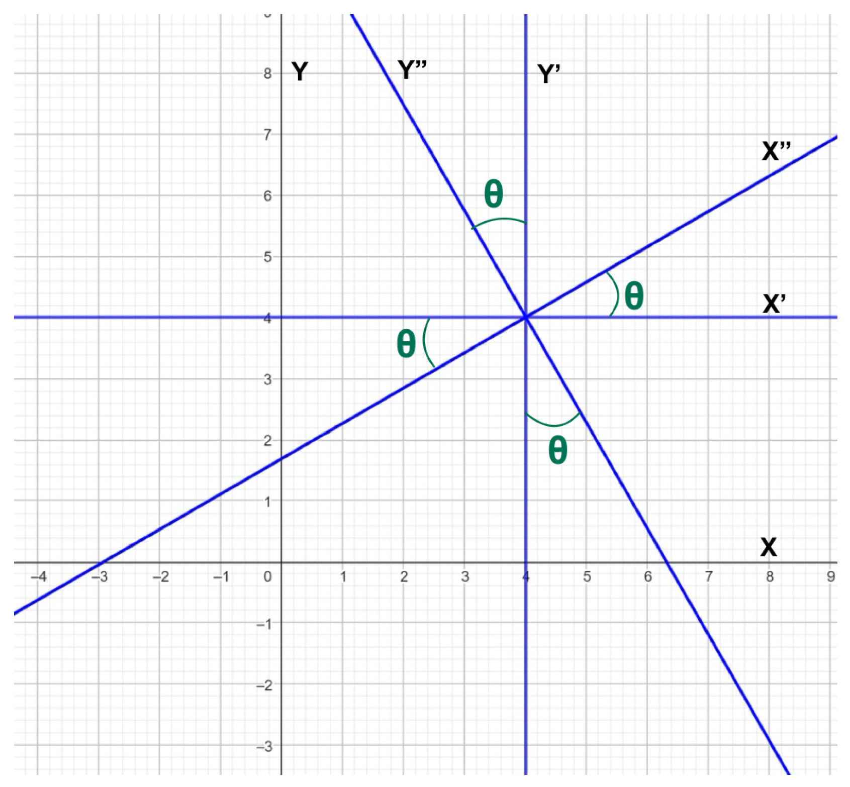
In (34)–(36), $x^{″}$ and $y^{″}$ correspond to the Cartesian axes generated by a rotation and a translation at the same time for some angle $\theta \in \left[0,{\displaystyle \frac{\pi }{2}}\right[$ and some translated origin $O^{\prime }(h,k)\in {\mathbb{R}}^2$. See Figure 9.

Figure 9. Translated and rotated Cartesian axes with respect to the original axes.

Proof. 

(i). Following pp. 137 and 140 in [3], if $d\ne 0$ in (1), then the equation without the translations of the locus in question is $A{\left(x^{\prime }\right)}^2+B{x}^{\prime }{y}^{\prime }+C{\left(y^{\prime }\right)}^2-{\displaystyle \frac{BDE-A{E}^2-C{D}^2-\left(B^2-4AC\right)F}{d}}=0$, where $x^{\prime }$ and $y^{\prime }$ correspond to the Cartesian axes translated to a new origin whose coordinates are $O^{\prime }(h,k)$ on the original Cartesian axes x and y. Now note that (11) implies ${\displaystyle \frac{BDE-A{E}^2-C{D}^2-\left(B^2-4AC\right)F}{d}}={\displaystyle \frac{4\Delta }{d}}.$ Thus, (1) is reduced to

$$A{\left(x^{\prime }\right)}^2+B{x}^{\prime }{y}^{\prime }+C{\left(y^{\prime }\right)}^2-{\displaystyle \frac{4\Delta }{d}}=0.$$

(37)

Now consider the following two possible cases:

Case 1. Suppose that (1) corresponds to an ellipse (degenerate or not) or a hyperbola (degenerate or not). Then, (17) reduces (37) to the form ${\displaystyle \frac{A+C+R}{2}}{\left(x^{\prime \prime }\right)}^2+{\displaystyle \frac{A+C-R}{2}}{\left(y^{\prime \prime }\right)}^2={\displaystyle \frac{4\Delta }{d}},$ which can also be rewritten as (34), where $x^{″}$ and $y^{″}$ correspond to new Cartesian axes whose origin is also $O^{\prime }$. Nevertheless, now they are also generated by some angle $\theta \in \left[0,{\displaystyle \frac{\pi }{2}}\right[$ with respect to the axes $x^{\prime }$ and $y^{\prime }$, as in Figure 9.

Case 2. If (1) corresponds to a circumference (degenerate or not), then Theorem 3(i) guarantees $R=0$, whereas $A=C$ and $B=0$; thus, ${\displaystyle \frac{A+C\pm R}{8}}={\displaystyle \frac{A+A\pm 0}{8}}={\displaystyle \frac{A}{4}}$. So, if we assume $\theta =0$, then ${\displaystyle \frac{A}{4}}{\left(x^{\prime }\right)}^2+{\displaystyle \frac{A}{4}}{\left(y^{\prime }\right)}^2={\displaystyle \frac{A+C+R}{8}}{\left(x^{″}\right)}^2+{\displaystyle \frac{A+C-R}{8}}{\left(y^{″}\right)}^2={\displaystyle \frac{\Delta }{d}}.$ Thus, $x^{\prime }=x^{″}$ and $y^{\prime }=y^{″}$.

(ii) Suppose $d=0$ and consider the only two possible cases for (2):

Case 1. If $A^{\prime }{\left(x^{\prime }\right)}^2+D^{\prime }{x}^{\prime }+E^{\prime }{y}^{\prime }+F=0$ with $A^{\prime }\ne C^{\prime }=0\ne E^{\prime }$, then its canonical form is given by ${\left(x^{\prime }+{\displaystyle \frac{D^{\prime }}{2A^{\prime }}}\right)}^2=-{\displaystyle \frac{E^{\prime }}{A^{\prime }}}\left(y^{\prime }-{\displaystyle \frac{{\left(D^{\prime }\right)}^2-4A^{\prime }F}{4A^{\prime }{E}^{\prime }}}\right)$, thus the parabola in question without rotations and translations is

$${\left(x^{″}\right)}^2=-{\displaystyle \frac{E^{\prime }}{A^{\prime }}}{y}^{″}.$$

(38)

Note that if (2) and (17) imply $C^{\prime }={\displaystyle \frac{A+C-R}{2}}=0$, then $R=A+C\ne 0$, which happens only when $\mathrm{sgn}\left(R\right)=\mathrm{sgn}\left(B\right)=\mathrm{sgn}(A+C)=\mathrm{sgn}\left(A\right)=\mathrm{sgn}\left(C\right)\ne 0$ for $B\ne 0$ due to Proposition 2, or when $\mathrm{sgn}\left(R\right)=\mathrm{sgn}\left(A\right)\ne \mathrm{sgn}\left(B\right)=\mathrm{sgn}\left(C\right)=0$ for $B=0$. So, $A^{\prime }={\displaystyle \frac{A+C+R}{2}}={\displaystyle \frac{A+C+A+C}{2}}=A+C\ne 0$ and $E^{\prime }=E\sqrt{{\displaystyle \frac{1}{2}}\left(1+{\displaystyle \frac{A-C}{R}}\right)}-D\sqrt{{\displaystyle \frac{1}{2}}\left(1-{\displaystyle \frac{A-C}{R}}\right)}=E\sqrt{{\displaystyle \frac{1}{2}}\left(1+{\displaystyle \frac{A-C}{A+C}}\right)}-D\sqrt{{\displaystyle \frac{1}{2}}\left(1-{\displaystyle \frac{A-C}{A+C}}\right)}=E\sqrt{{\displaystyle \frac{A}{A+C}}}-D\sqrt{{\displaystyle \frac{C}{A+C}}}\ne 0$. Hence, $-{\displaystyle \frac{E^{\prime }}{A^{\prime }}}={\displaystyle \frac{1}{A+C}}\left(D\sqrt{{\displaystyle \frac{C}{A+C}}}-E\sqrt{{\displaystyle \frac{A}{A+C}}}\right)\ne 0$; thus, (38) becomes (35).

Case 2. If $C^{\prime }{\left(y^{\prime }\right)}^2+D^{\prime }{x}^{\prime }+E^{\prime }{y}^{\prime }+F=0$ with $C^{\prime }\ne A^{\prime }=0\ne D^{\prime }$, then its canonical form is given by ${\left(y^{\prime }+{\displaystyle \frac{E^{\prime }}{2C^{\prime }}}\right)}^2=-{\displaystyle \frac{D^{\prime }}{C^{\prime }}}\left(x^{\prime }-{\displaystyle \frac{{\left(E^{\prime }\right)}^2-4C^{\prime }F}{4C^{\prime }{D}^{\prime }}}\right)$; thus, the parabola in question without rotations and translations is

$${\left(y^{″}\right)}^2=-{\displaystyle \frac{D^{\prime }}{A^{\prime }}}{x}^{″}.$$

(39)

Note that if (2) and (17) imply $A^{\prime }={\displaystyle \frac{A+C+R}{2}}=0$, then $R=-(A+C)\ne 0$, which happens only when $\mathrm{sgn}\left(R\right)=\mathrm{sgn}\left(B\right)=-\mathrm{sgn}(A+C)=-\mathrm{sgn}\left(A\right)=-\mathrm{sgn}\left(C\right)\ne 0$ for $B\ne 0$ due to Proposition 2, or when $\mathrm{sgn}\left(C\right)=-\mathrm{sgn}\left(R\right)\ne \mathrm{sgn}\left(A\right)=\mathrm{sgn}\left(B\right)=0$ for $B=0$. So, $C^{\prime }={\displaystyle \frac{A+C-R}{2}}={\displaystyle \frac{A+C-[-(A+C\left)\right]}{2}}=A+C\ne 0$ and $D^{\prime }=D\sqrt{{\displaystyle \frac{1}{2}}\left(1+{\displaystyle \frac{A-C}{R}}\right)}+E\sqrt{{\displaystyle \frac{1}{2}}\left(1-{\displaystyle \frac{A-C}{R}}\right)}=D\sqrt{{\displaystyle \frac{1}{2}}\left[1+{\displaystyle \frac{A-C}{-(A+C)}}\right]}+E\sqrt{{\displaystyle \frac{1}{2}}\left[1-{\displaystyle \frac{A-C}{-(A+C)}}\right]}=D\sqrt{{\displaystyle \frac{C}{A+C}}}+E\sqrt{{\displaystyle \frac{A}{A+C}}}\ne 0$. Hence, $-{\displaystyle \frac{D^{\prime }}{A^{\prime }}}=-{\displaystyle \frac{1}{A+C}}\left(D\sqrt{{\displaystyle \frac{C}{A+C}}}+E\sqrt{{\displaystyle \frac{A}{A+C}}}\right)\ne 0$; thus, (39) becomes (36). □

Theorem 4 also works for $h=k=0$, whereas (34) makes evident that (1) corresponds to degenerate cases of circumferences, ellipses, and hyperbolas whenever $\Delta =0\ne d$ (see p. 137 in [3]). Additionally, note that while (17) does not work for the circumference because $R=0$ for this locus, Theorem 4(i) covers this case with no regard to the value of R. Likewise, the following result states a general criterion to identify a priori the degenerate cases of the parabola. It is conceived as a follow-up of Lemma 1.

Corollary 4

(Second Theorem of the Non-Degenerate Parabola). Let $A,B,C,D,E,F\in \mathbb{R}$ be such that at least one of the first three of them is non-null. If $d=0$, then the equation $A{x}^2+Bxy+C{y}^2+Dx+Ey+F=0$ corresponds to a non-degenerate parabola if and only if $A{E}^2\ne C{D}^2$.

Proof. 

Note that Theorem 4(ii) implies that (1) corresponds to a degenerate case of the parabola if and only if ${\displaystyle \frac{1}{A+C}}\left(D\sqrt{{\displaystyle \frac{C}{A+C}}}-E\sqrt{{\displaystyle \frac{A}{A+C}}}\right)=0$, or $-{\displaystyle \frac{1}{A+C}}\left(D\sqrt{{\displaystyle \frac{C}{A+C}}}+E\sqrt{{\displaystyle \frac{A}{A+C}}}\right)=0$, so $\left[{\displaystyle \frac{1}{A+C}}\left(D\sqrt{{\displaystyle \frac{C}{A+C}}}-E\sqrt{{\displaystyle \frac{A}{A+C}}}\right)\right]\left[-{\displaystyle \frac{1}{A+C}}\left(D\sqrt{{\displaystyle \frac{C}{A+C}}}+E\sqrt{{\displaystyle \frac{A}{A+C}}}\right)\right]={\displaystyle \frac{A{E}^2-C{D}^2}{{(A+C)}^3}}=0$. This ensures that (1) corresponds to a non-degenerate parabola whenever $A{E}^2\ne C{D}^2$. □

Example 11.

Consider the equation given in Example 2, in which $d=0$ and $A{E}^2=\left(9\right){(-60)}^2=32400\ne C{D}^2=\left(16\right){\left(80\right)}^2=102400$. This reaffirms that this equation corresponds to a non-degenerate parabola according to Corollary 4. On the other hand, $\mathrm{sgn}\left(A\right)=\mathrm{sgn}\left(9\right)=\mathrm{sgn}\left(R\right)=\mathrm{sgn}\left(25\right)=1\ne 0$ in Example 2; therefore, Theorem 4(ii) yields ${\left(x^{\prime \prime }\right)}^2={\displaystyle \frac{1}{9+16}}\left[80\sqrt{{\displaystyle \frac{16}{9+16}}}-(-60)\sqrt{{\displaystyle \frac{9}{9+16}}}\right]y^{″}=4y^{″}$. This is equivalent to the result given by (17). On the other hand, note that Corollary 4 also reaffirms Example 7 as a degenerate case of the parabola due to $d=0$ and $A{E}^2=a^2{\left(2bc\right)}^2=4a^2{b}^2{c}^2=b^2{\left(2ac\right)}^2=C{D}^2$ in (22).

6. General Features of the Conic Sections

6.1. Eccentricity

According to [14], if (1) corresponds to an ellipse or a hyperbola, then the eccentricity of these loci is given by $\epsilon =\sqrt{{\displaystyle \frac{2\sqrt{{(A-C)}^2+B^2}}{\eta (A+C)+\sqrt{{(A-C)}^2+B^2}}}}$, where $\eta =\left\{\begin{array}{c}1, \mathrm{if} \Delta <0\\ -1, \mathrm{if} \Delta >0.\end{array}\right.$ However, although this formula is absolutely true, it presents a small redundancy on the use of $\eta$; so, we devote this subsection to providing greater clarity on this formula. We begin by exposing the following lemma before presenting the main result of this subsection.

Lemma 2

(Theorem of the Equilateral Hyperbola). Let $A,B,C,D,E,F\in \mathbb{R}$ be such that $A{x}^2+Bxy+C{y}^2+Dx+Ey+F=0$ corresponds to a non-degenerate hyperbola. Then,

(i)  This hyperbola is equilateral if and only if $C=-A$.

(ii)  This hyperbola is equilateral if and only if its eccentricity is $\epsilon =\sqrt{2}.$

Proof. 

(i) Case 1. Suppose that $B=0$, then (1) corresponds to an equilateral hyperbola if and only if there exist $h,k\in \mathbb{R}$ and $a>0$, such that the canonical form of this locus is given by ${\displaystyle \frac{{(x-h)}^2}{a^2}}-{\displaystyle \frac{{(y-k)}^2}{a^2}}=\pm 1.$ So, the general form of such a hyperbola is $A{x}^2-A{y}^2-2Ahx+2Aky+A\left(h^2-k^2\mp a^2\right)=0$ for some $A\in \mathbb{R}\setminus \left\{0\right\}$. Therefore, $C=-A$.

Case 2. Suppose that $B\ne 0$, then Case 1 guarantees that (1) and (2) correspond to an equilateral hyperbola if and only if $C^{\prime }=-A^{\prime }\ne 0$ in (2). So, since Corollary 2(i) guarantees $A^{\prime }+C^{\prime }=A+C=0$, the conclusion of Case 1 can also be extended to this case.

(ii) According to pp. 194 and 211 in [2], the eccentricity of any hyperbola is given by $\epsilon ={\displaystyle \frac{c}{a}}>1$ and $c=\sqrt{a^2+b^2}>0.$ So, (1) corresponds to an equilateral hyperbola when $a=b>0$. This ensures $a^2+b^2=2a^2>0$. Therefore, $\epsilon ={\displaystyle \frac{c}{a}}={\displaystyle \frac{\sqrt{a^2+b^2}}{a}}=\sqrt{{\displaystyle \frac{2a^2}{a^2}}}=\sqrt{2}$ □

Theorem 5

(The General Formulae for the Eccentricity of Conic Sections). Let A, B, C, D, E, $F\in \mathbb{R}$ be such that $A{x}^2+Bxy+C{y}^2+Dx+Ey+F=0$ corresponds to a non-degenerate locus on the Cartesian plane, and let R be its respective conic radical. Then,

(i) If this locus is a circumference, a parabola, an ellipse, or an equilateral hyperbola, then its eccentricity is $\epsilon =\sqrt{{\displaystyle \frac{2\left|R\right|}{|A+C|+\left|R\right|}}}$.

(ii) If this locus is a non-equilateral hyperbola, then its eccentricity is $\epsilon =\sqrt{{\displaystyle \frac{2\left|R\right|}{-\mathrm{sgn}(\Delta )(A+C)+\left|R\right|}}}$.

Proof. 

(i) Case 1. Suppose that (1) corresponds to a non-degenerate circumference. Then, $A=C\ne 0=B$ and $\epsilon =0$ (see p. 124 in [8]). Since Theorem 3(i) ensures that $R=0$, $\sqrt{{\displaystyle \frac{2\left|R\right|}{|A+C|+\left|R\right|}}}=\sqrt{{\displaystyle \frac{2\left|0\right|}{|A+A|+\left|0\right|}}}=\sqrt{{\displaystyle \frac{0}{2\left|A\right|}}}=0=\epsilon$.

Case 2. Suppose that (1) corresponds to a non-degenerate parabola. Then, $\epsilon =1$ (see p. 211 in [2]). Moreover, Propositions 1(iv) and 2(ii) and Theorem 3(ii) imply $\left|R\right|=\sqrt{{(A-C)}^2+B^2}=|A+C|\ne 0.$ Therefore, $\sqrt{{\displaystyle \frac{2\left|R\right|}{|A+C|+\left|R\right|}}}=\sqrt{{\displaystyle \frac{2|A+C|}{|A+C|+|A+C|}}}=1=\epsilon .$

Case 3. Suppose that (1) corresponds to an equilateral hyperbola, then there are two possibilities: $A\ne B=0$ for the non-rotated case and $B\ne 0$ for the rotated case. Hence, it is clear that $4A^2+B^2>0$ for both possibilities. Therefore, Proposition 1(iv) and Lemma 2 guarantee the following relation: $\sqrt{{\displaystyle \frac{2\left|R\right|}{|A+C|+\left|R\right|}}}=\sqrt{{\displaystyle \frac{2\sqrt{{(A-C)}^2+B^2}}{|A+C|+\sqrt{{(A-C)}^2+B^2}}}}=\sqrt{{\displaystyle \frac{2\sqrt{{(A+A)}^2+B^2}}{|A-A|+\sqrt{{(A+A)}^2+B^2}}}}=\sqrt{{\displaystyle \frac{2\sqrt{4A^2+B^2}}{\sqrt{4A^2+B^2}}}}=\sqrt{2}=\epsilon$.

Case 4. Suppose that (1) corresponds to a non-degenerate ellipse, then $\epsilon ={\displaystyle \frac{c}{a}}=\sqrt{{\displaystyle \frac{a^2-b^2}{a^2}}}$ (see p. 176 in [2]), whereas (17) guarantees $R\ne 0$ and Theorem 4(i) implies that the canonical equation of this locus is

$${\displaystyle \frac{{\left(x^{″}\right)}^2}{\left(\frac{4\Delta }{A^{\prime }d}\right)}}+{\displaystyle \frac{{\left(y^{″}\right)}^2}{\left(\frac{4\Delta }{C^{\prime }d}\right)}}=1,$$

(40)

where $A^{\prime }={\displaystyle \frac{A+C+R}{2}}$ and $C^{\prime }={\displaystyle \frac{A+C-R}{2}}$, and $\Delta \ne 0>d$, according to Corollary 3(i). So, (40) implies the following two complementary subcases.

Subcase A. If $a=\sqrt{{\displaystyle \frac{4\Delta }{A^{\prime }d}}}>b=\sqrt{{\displaystyle \frac{4\Delta }{C^{\prime }d}}}>0,$ then $C^{\prime }={\displaystyle \frac{A+C-R}{2}}>A^{\prime }={\displaystyle \frac{A+C+R}{2}}>0$ when $\mathrm{sgn}\left(d\right)=\mathrm{sgn}(\Delta )=-1$ and $C^{\prime }={\displaystyle \frac{A+C-R}{2}}<A^{\prime }={\displaystyle \frac{A+C+R}{2}}<0$ when $-\mathrm{sgn}\left(d\right)=\mathrm{sgn}(\Delta )=1$. Thus, $A+C>-R>0>R$ when $\mathrm{sgn}\left(d\right)=\mathrm{sgn}(\Delta )=-1$, or $R>0>-R>A+C$ when $-\mathrm{sgn}\left(d\right)=\mathrm{sgn}(\Delta )=1$. Hence, $-\mathrm{sgn}(A+C)=\mathrm{sgn}\left(R\right)\ne 0$ in general for this subcase. Therefore, Property 1 implies that the eccentricity in this subcase is $\epsilon =\sqrt{{\displaystyle \frac{a^2-b^2}{a^2}}}=\sqrt{{\displaystyle \frac{\frac{4\Delta }{A^{\prime }d}-\frac{4\Delta }{C^{\prime }d}}{\frac{4\Delta }{A^{\prime }d}}}}=\sqrt{{\displaystyle \frac{C^{\prime }-A^{\prime }}{C^{\prime }}}}=\sqrt{{\displaystyle \frac{\frac{A+C-R}{2}-\frac{A+C+R}{2}}{\frac{A+C-R}{2}}}}=\sqrt{{\displaystyle \frac{2R}{-(A+C)+R}}}=\sqrt{{\displaystyle \frac{2\mathrm{sgn}\left(R\right)\left|R\right|}{-\mathrm{sgn}(A+C)|A+C|+\mathrm{sgn}\left(R\right)\left|R\right|}}}=\sqrt{{\displaystyle \frac{2\mathrm{sgn}\left(R\right)\left|R\right|}{\mathrm{sgn}\left(R\right)|A+C|+\mathrm{sgn}\left(R\right)\left|R\right|}}}=\sqrt{{\displaystyle \frac{2\left|R\right|}{|A+C|+\left|R\right|}}}$.

Subcase B. If $a=\sqrt{{\displaystyle \frac{4\Delta }{C^{\prime }d}}}>b=\sqrt{{\displaystyle \frac{4\Delta }{A^{\prime }d}}}>0,$ then $A^{\prime }={\displaystyle \frac{A+C+R}{2}}>C^{\prime }={\displaystyle \frac{A+C-R}{2}}>0$ when $\mathrm{sgn}\left(d\right)=\mathrm{sgn}(\Delta )=-1$ and $A^{\prime }={\displaystyle \frac{A+C+R}{2}}<C^{\prime }={\displaystyle \frac{A+C-R}{2}}<0$ when $-\mathrm{sgn}\left(d\right)=\mathrm{sgn}(\Delta )=1$. Thus, $A+C>R>0>-R$ when $\mathrm{sgn}\left(d\right)=\mathrm{sgn}(\Delta )=-1$, or $-R>0>R>A+C$ when $-\mathrm{sgn}\left(d\right)=\mathrm{sgn}(\Delta )=1$. Hence, $\mathrm{sgn}(A+C)=\mathrm{sgn}\left(R\right)\ne 0$ in general for this subcase. Therefore, Property 1 implies that the eccentricity is $\epsilon =\sqrt{{\displaystyle \frac{a^2-b^2}{a^2}}}=\sqrt{{\displaystyle \frac{\frac{4\Delta }{C^{\prime }d}-\frac{4\Delta }{A^{\prime }d}}{\frac{4\Delta }{C^{\prime }d}}}}=\sqrt{{\displaystyle \frac{A^{\prime }-C^{\prime }}{A^{\prime }}}}=\sqrt{{\displaystyle \frac{\frac{A+C+R}{2}-\frac{A+C-R}{2}}{\frac{A+C+R}{2}}}}=\sqrt{{\displaystyle \frac{2R}{A+C+R}}}=\sqrt{{\displaystyle \frac{2\mathrm{sgn}\left(R\right)\left|R\right|}{\mathrm{sgn}(A+C)|A+C|+\mathrm{sgn}\left(R\right)\left|R\right|}}}=\sqrt{{\displaystyle \frac{2\mathrm{sgn}\left(R\right)\left|R\right|}{\mathrm{sgn}\left(R\right)|A+C|+\mathrm{sgn}\left(R\right)\left|R\right|}}}=\sqrt{{\displaystyle \frac{2\left|R\right|}{|A+C|+\left|R\right|}}}$.

(ii) Suppose that (1) corresponds to a non-degenerate and non-equilateral hyperbola. Then, $\epsilon ={\displaystyle \frac{c}{a}}=\sqrt{{\displaystyle \frac{a^2+b^2}{a^2}}}$ (see p. 194 in [2]). Hence, (17) guarantees $R\ne 0$ and Corollary 3(i) yields $d>0$. So, (40) implies the following two complementary cases.

Case 1. Suppose that $a=\sqrt{{\displaystyle \frac{4\Delta }{A^{\prime }d}}}>0$ and $b=\sqrt{-{\displaystyle \frac{4\Delta }{C^{\prime }d}}}>0$. So, if $\Delta >0$ then $A^{\prime }={\displaystyle \frac{A+C+R}{2}}>0>C^{\prime }={\displaystyle \frac{A+C-R}{2}}$. This implies $A^{\prime }-C^{\prime }=R>0$ and, thus, $\mathrm{sgn}\left(R\right)=\mathrm{sgn}(\Delta )=1$. However, if $\Delta <0$, then $A^{\prime }={\displaystyle \frac{A+C+R}{2}}<0<C^{\prime }={\displaystyle \frac{A+C-R}{2}}$. This implies $A^{\prime }-C^{\prime }=R<0$ and, thus, $\mathrm{sgn}\left(R\right)=\mathrm{sgn}(\Delta )=-1$. Hence, it is clear that $\mathrm{sgn}\left(R\right)\mathrm{sgn}(\Delta )=1$ in this case. Therefore, Property 1 yields that $\epsilon =\sqrt{{\displaystyle \frac{a^2+b^2}{a^2}}}=\sqrt{{\displaystyle \frac{\frac{4\Delta }{A^{\prime }d}+\left(-\frac{4\Delta }{C^{\prime }d}\right)}{\frac{4\Delta }{A^{\prime }d}}}}=\sqrt{{\displaystyle \frac{C^{\prime }-A^{\prime }}{C^{\prime }}}}=\sqrt{{\displaystyle \frac{2R}{-(A+C)+R}}}=\sqrt{{\displaystyle \frac{2\mathrm{sgn}\left(R\right)\left|R\right|}{-\mathrm{sgn}\left(R\right)\mathrm{sgn}(\Delta )(A+C)+\mathrm{sgn}\left(R\right)\left|R\right|}}}=\sqrt{{\displaystyle \frac{2\left|R\right|}{-\mathrm{sgn}(\Delta )(A+C)+\left|R\right|}}}$.

Case 2. Suppose that $a=\sqrt{{\displaystyle \frac{4\Delta }{C^{\prime }d}}}>0$ and $b=\sqrt{-{\displaystyle \frac{4\Delta }{A^{\prime }d}}}>0$. So, if $\Delta >0$, then $C^{\prime }={\displaystyle \frac{A+C-R}{2}}>0>A^{\prime }={\displaystyle \frac{A+C+R}{2}}$. This implies $A^{\prime }-C^{\prime }=R<0$ and, thus, $\mathrm{sgn}\left(R\right)=-\mathrm{sgn}(\Delta )=-1$. However, if $\Delta <0$, then $C^{\prime }={\displaystyle \frac{A+C-R}{2}}<0<A^{\prime }={\displaystyle \frac{A+C+R}{2}}$. This implies $A^{\prime }-C^{\prime }=R>0$ and, thus, $\mathrm{sgn}\left(R\right)=-\mathrm{sgn}(\Delta )=1$. Hence, it is clear that $-\mathrm{sgn}\left(R\right)\mathrm{sgn}(\Delta )=1$ in this case. Therefore, Property 1 yields that $\epsilon =\sqrt{{\displaystyle \frac{a^2+b^2}{a^2}}}=\sqrt{{\displaystyle \frac{\frac{4\Delta }{C^{\prime }d}+\left(-\frac{4\Delta }{A^{\prime }d}\right)}{\frac{4\Delta }{C^{\prime }d}}}}=\sqrt{{\displaystyle \frac{A^{\prime }-C^{\prime }}{A^{\prime }}}}=\sqrt{{\displaystyle \frac{2R}{A+C+R}}}=\sqrt{{\displaystyle \frac{2\mathrm{sgn}\left(R\right)\left|R\right|}{-\mathrm{sgn}\left(R\right)\mathrm{sgn}(\Delta )(A+C)+\mathrm{sgn}\left(R\right)\left|R\right|}}}=\sqrt{{\displaystyle \frac{2\left|R\right|}{-\mathrm{sgn}(\Delta )(A+C)+\left|R\right|}}}$. □

Example 12.

Consider $R_1=-28$ from Example 1. Then, Theorem 5(i) yields ${\epsilon }_1=\sqrt{{\displaystyle \frac{2|-28|}{|43+57|+|-28|}}}={\displaystyle \frac{\sqrt{7}}{4}}.$ Note also that the canonical equation ${\displaystyle \frac{{(x^{\prime }-1)}^2}{16}}+{\displaystyle \frac{{\left(y^{\prime }\right)}^2}{9}}=1$ implies $a^2=16$ and $b^2=9$. Thus, ${\epsilon }_1=\sqrt{{\displaystyle \frac{16-9}{16}}}={\displaystyle \frac{\sqrt{7}}{4}}$ verifies our claim. Now consider $R_2=25$ from Example 2. Then, Theorem 5(i) yields ${\epsilon }_2=\sqrt{{\displaystyle \frac{2\left|25\right|}{|9+16|+\left|25\right|}}}=1.$ This corresponds to the eccentricity of any parabola. Finally, Lemma 2(i) guarantees that the hyperbola of Example 3 is equilateral due to $A=-C=0$, so Theorem 5(i) guarantees that it is not necessary to obtain $\mathrm{sgn}(\Delta )$ to compute the eccentricity in this example due to $R_3=1$ implying ${\epsilon }_3=\sqrt{{\displaystyle \frac{2\left|1\right|}{(0+0)+\left|1\right|}}}=\sqrt{2}$, which coincides with the result given by Lemma 2(ii). Additionally, observe that the canonical equation ${\displaystyle \frac{{\left(x^{\prime }\right)}^2}{2}}-{\displaystyle \frac{{\left(y^{\prime }\right)}^2}{2}}=1$ implies $a^2=b^2=2$; and, thus, ${\epsilon }_3=\sqrt{{\displaystyle \frac{2+2}{2}}}=\sqrt{2}$ verifies our claim.

Example 13.

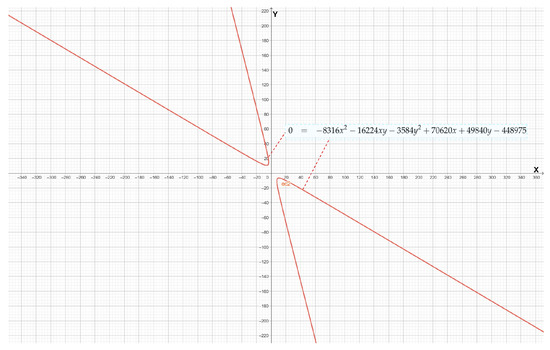
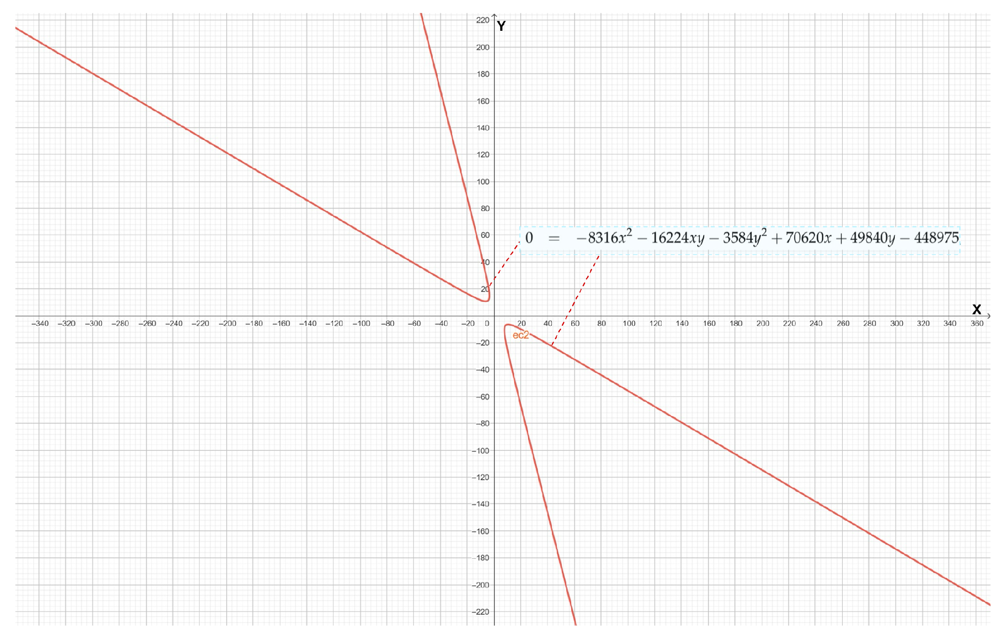
Let $-8316x^2-16,224xy-3584y^2+70,620x+49,840y-448,975=0$, then $d=144,000,000>0$ and $\Delta =$ 11,520,000,000,000 > 0, so $\mathrm{sgn}(\Delta )=1$. Thus, Corollary 3(iii) implies that the given equation corresponds to a rotated hyperbola (see Figure 10).

Figure 10. Plot of $-8316x^2-16,224xy-3584y^2+70,620x+49,840y-448975=0$.

In addition, note that $R=\mathrm{sgn}(-16224)\sqrt{{[-8316-(-3584)]}^2+{(-16224)}^2}=-16900.$ Then, Theorem 5(ii) implies $\epsilon =\sqrt{{\displaystyle \frac{2|-16900|}{-\left(1\right)[-8316+(-3584\left)\right]+|-16900|}}}={\displaystyle \frac{13}{12}}$. On the other hand, if we apply (34) to the given equation, then we obtain $-3600{\left(x^{″}\right)}^2+625{\left(y^{″}\right)}^2=80000$, whose canonical form is ${\displaystyle \frac{{\left(y^{″}\right)}^2}{128}}-{\displaystyle \frac{{\left(x^{″}\right)}^2}{\left(\frac{200}{9}\right)}}=1.$ Hence, $a^2=128$ and $b^2={\displaystyle \frac{200}{9}}$, so $\epsilon =\sqrt{{\displaystyle \frac{128+\frac{200}{9}}{128}}}={\displaystyle \frac{13}{12}}$, which verifies our claim.

Example 14.

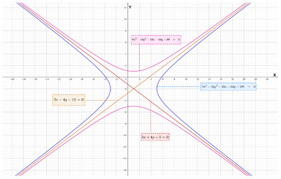
Consider the equations

$$\begin{array}{ccc}\hfill 9x^2-16y^2-18x-64y-199& =& 0,\hfill \end{array}$$

(41)

$$\begin{array}{ccc}\hfill 9x^2-16y^2-18x-64y+89& =& 0;\hfill \end{array}$$

(42)

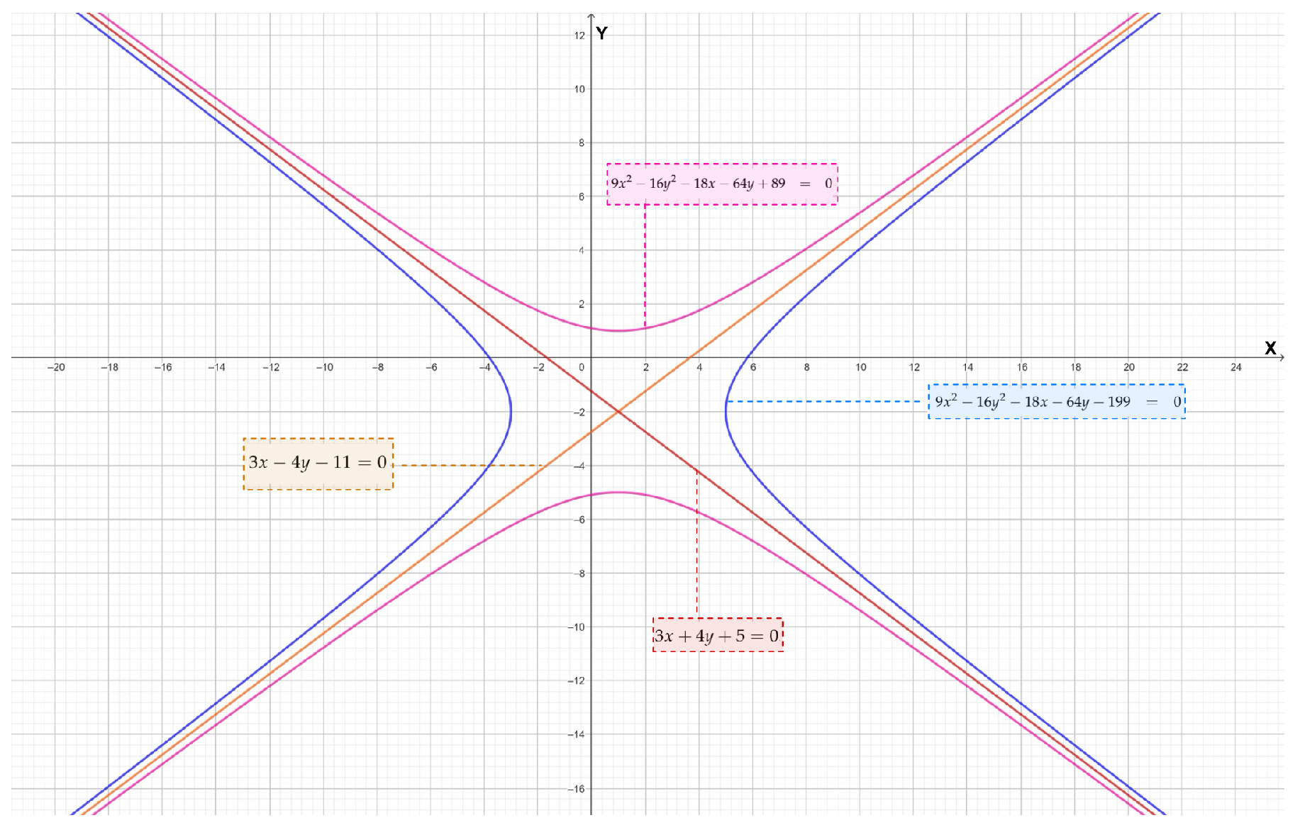
Then, by (11), their respective Conic Determinants are ${\Delta }_1=20736>0$ and ${\Delta }_2=-20736<0$, so $\mathrm{sgn}\left({\Delta }_1\right)=1$ and $\mathrm{sgn}\left({\Delta }_2\right)=-1$. Also, $d_1=d_2=576>0$; thus, ${\Delta }_1\ne 0\ne {\Delta }_2$, Lemma 2(i), and Corollary 3(iii) imply that (41)–(42) correspond to a couple of non-equilateral hyperbolas. Therefore, if $R_1=R_2=9-(-16)=25$, then Theorem 5(ii) implies that the respective eccentricities of these hyperbolas are ${\epsilon }_1=\sqrt{{\displaystyle \frac{2\left|25\right|}{-\left(1\right)[9+(-16\left)\right]+\left|25\right|}}}={\displaystyle \frac{5}{4}}$ and ${\epsilon }_2=\sqrt{{\displaystyle \frac{2\left|25\right|}{-(-1)[9+(-16\left)\right]+\left|25\right|}}}={\displaystyle \frac{5}{3}}.$ On the other hand, the respective canonical forms of (41)–(42) are

$$\begin{array}{ccc}\hfill {\displaystyle \frac{{(x-1)}^2}{16}}-{\displaystyle \frac{{(y+2)}^2}{9}}& =& 1,\hfill \end{array}$$

(43)

$$\begin{array}{ccc}\hfill {\displaystyle \frac{{(y+2)}^2}{9}}-{\displaystyle \frac{{(x-1)}^2}{16}}& =& 1.\hfill \end{array}$$

(44)

Hence, (43) implies $a_1^2=16$ and $b_1^2=9$, so ${\epsilon }_1=\sqrt{{\displaystyle \frac{16+9}{16}}}={\displaystyle \frac{5}{4}}$; meanwhile, (44) implies $a_2^2=9$ and $b_2^2=16$, so ${\epsilon }_2=\sqrt{{\displaystyle \frac{16+9}{9}}}={\displaystyle \frac{5}{3}}$, which verify our claims regarding the use of Theorem 5(ii). Figure 11 shows how (41)–(42) have the same pair of asymptotes.

Figure 11. Plot of (41)–(42) and their two asymptotes: $3x-4y-11=0$ and $3x+4y+5=0$.

Theorem 5 refines Ayoub’s eccentricity formula by showing that $\mathrm{sgn}(\Delta )$ is only necessary for non-equilateral hyperbolas. While $\mathrm{sgn}(\Delta )$ is generally required in [14], Theorem 5 proves otherwise because hyperbolas uniquely exhibit a duality: each family of hyperbolas has a conjugate family sharing the same asymptotes. In such cases, $\mathrm{sgn}(\Delta )$ distinguishes which family corresponds to the given equation. In contrast, for equilateral hyperbolas, both conjugate families have identical eccentricities (Lemma 2(ii)), making $\mathrm{sgn}(\Delta )$ irrelevant, so the same applies to the other conic sections, as they lack this ambiguity. Thus, Theorem 5 generalizes the eccentricity formula by reducing dependency on $\mathrm{sgn}(\Delta )$. Example 14 and Figure 11 illustrate this, showing two conjugate hyperbolas derived from equations that differ only in the sign of $\Delta$ yet share asymptotes.

6.2. Taxonomy of the Conic Sections in ${\mathbb{R}}^2$

Theorem 6.

Let $A,B,C,D,E,F\in \mathbb{R}$ be such that at least one of the first five of these numbers is non-zero. Then, all the loci represented by the equation $A{x}^2+Bxy+C{y}^2+Dx+Ey+F=0$ are classified into the following five families, depending on the values of all its coefficients:

(A)  The family of single straight lines ($d=\Delta =0$):

(i)  Standard straight lines: This case corresponds to all the single straight lines on the Cartesian plane that are non-parallel to any Cartesian axes. So, this happens if and only if $A=B=C=0$ and $D\ne 0\ne E$.

(ii)  Horizontal straight lines: This case corresponds to all the single straight lines that are parallel to the x-axis on the Cartesian plane. So, this happens if and only if $A=B=C=0$ and $D=0\ne E$.

(iii)  Vertical straight lines: This case corresponds to all the single straight lines that are parallel to the y-axis on the Cartesian plane. So, this happens if and only if $A=B=C=0$ and $D\ne 0=E$.

(B)  The family of circumferences ($d<0$):

(iv)  Non-degenerate circumferences: This happens if and only if $A=C,B=0$ and $\mathrm{sgn}\left(A\right)=-\mathrm{sgn}(\Delta )\ne 0.$

(v)  Circumferential single points: This is the only degenerate case of the circumference, which corresponds to all the general circumference equations that represent single points on the Cartesian plane. So, this happens if and only if $A=C\ne B=0=\Delta$.

(vi)  Imaginary circumferences: This case corresponds to all the general equations of the circumference that do not have a graphical representation on the Cartesian plane. So, this happens if and only if $A=C,B=0$ and $\mathrm{sgn}\left(A\right)=\mathrm{sgn}(\Delta )\ne 0.$

(C)  The parabolic family ($d=0$):

(vii)  Non-degenerate parabolas: This case happens if and only if $d=0$ and $A{E}^2\ne C{D}^2$, whereas $2AE\ne BD$ or $2CD\ne BE$.

(viii)  Couples of parallel straight lines: This is the first degenerate case of the parabola, which corresponds to all the couples of different straight lines with the same slope on the Cartesian plane. So, this happens if and only if $d=A{E}^2-C{D}^2=2AE-BD=2CD-BE=0<\left|A\right|+\left|B\right|+\left|C\right|$ with $D^2-4AF>0$ or with $E^2-4CF>0.$

(ix)  Duplicated straight lines: This is the second degenerate case of the parabola, which consists of all the equations that correspond to a couple of straight lines that are, in fact, the same one on the Cartesian plane. So, this happens if and only if $d=A{E}^2-C{D}^2=2AE-BD=2CD-BE=0<\left|A\right|+\left|B\right|+\left|C\right|$ with $D^2-4AF=0$ or with $E^2-4CF=0.$

(x)  Couples of parallel imaginary lines: This case corresponds to all the couples of “imaginary” straight lines with the same real or undefined slope, whose respective independent terms are a couple of conjugate complex numbers. Thus, these straight lines do not have a graphical representation on the Cartesian plane. So, this happens if and only if $d=A{E}^2-C{D}^2=2AE-BD=2CD-BE=0$ with $D^2-4AF<0$ or with $E^2-4CF<0.$

(D)  The elliptical family ($d<0$):

(xi)  Non-degenerate ellipses: This case happens if and only if $\mathrm{sgn}\left(A\right)=-\mathrm{sgn}(\Delta )\ne 0$ with $A-C\ne B=0$ and $\mathrm{sgn}\left(A\right)=\mathrm{sgn}\left(C\right)$, or with $B\ne 0>d$.

(xii)  Elliptical single points: This is the only degenerate case of the ellipse, which corresponds to all the equations that also represent single points on the Cartesian plane, but they do not satisfy the conditions of (v) above. So, this happens if and only if $A-C\ne B=\Delta =0\ne \mathrm{sgn}\left(A\right)=\mathrm{sgn}\left(C\right)$ or $B\ne \Delta =0>d.$

(xiii)  Imaginary ellipses: This case corresponds to all the equations that do not have a graphical representation on the Cartesian plane and are also different from Cases (vi) and (x). So, this happens if and only if $\mathrm{sgn}\left(A\right)=\mathrm{sgn}(\Delta )\ne 0$ with $A-C\ne B=0$ and $\mathrm{sgn}\left(A\right)=\mathrm{sgn}\left(C\right)$, or with $B\ne 0>d.$

(E)  The hyperbolic family ($d>0$):

(xiv)  Non-degenerate hyperbolas: This case happens if and only if $d>0\ne \Delta$.

(xv)  Couples of non-parallel straight lines: This is the only degenerate case of the hyperbola, which corresponds to all the couples of straight lines on the Cartesian plane whose slopes are different among them. So, this happens if and only if $d>0=\Delta .$

Before we proceed with the proof of this result, we introduce an ancillary one.

Lemma 3.

Let $A,B,C\in \mathbb{R}$ be such that $B^2-4AC<0$. Then,

• (i)  $\mathrm{sgn}\left(A\right)=\mathrm{sgn}\left(C\right)=\mathrm{sgn}(A+C)\ne 0$.
• (ii)  $|A+C|>\left|R\right|$.
• (iii)  If $A^{\prime }={\displaystyle \frac{A+C+R}{2}},C^{\prime }={\displaystyle \frac{A+C-R}{2}}$, then $\mathrm{sgn}\left(A\right)=\mathrm{sgn}\left(A^{\prime }\right)=\mathrm{sgn}\left(C^{\prime }\right)=\mathrm{sgn}(A^{\prime }+C^{\prime })\ne 0$.

Proof. 

(i). If $B^2-4AC<0$, then $0\le B^2<4AC$; thus, $AC>0$, so $\mathrm{sgn}\left(A\right)=\mathrm{sgn}\left(C\right)\ne 0$; hence, what remains of the proof is identical to that of Proposition 2(iii).

• (ii) If $B^2<4AC$, then $R^2={(A-C)}^2+B^2<A^2-2AC+C^2+4AC={(A+C)}^2$. Thus, $|A+C|>\left|R\right|$.
• (iii) If $A+C>0$, then (ii) implies $A+C>\pm R$, which guarantees $A^{\prime }={\displaystyle \frac{A+C+R}{2}}>0$ and $C^{\prime }={\displaystyle \frac{A+C-R}{2}}>0$; hence, $\mathrm{sgn}(A+C)=\mathrm{sgn}\left(A^{\prime }\right)=\mathrm{sgn}\left(C^{\prime }\right)=1$. On the other hand, if $A+C<0$, then (ii) implies $A+C<\pm R$, which guarantees $A^{\prime }={\displaystyle \frac{A+C+R}{2}}<0$ and $C^{\prime }={\displaystyle \frac{A+C-R}{2}}<0$; hence, $\mathrm{sgn}(A+C)=\mathrm{sgn}\left(A^{\prime }\right)=\mathrm{sgn}\left(C^{\prime }\right)=-1$. Therefore, (i) guarantees $\mathrm{sgn}\left(A\right)=\mathrm{sgn}\left(A^{\prime }\right)=\mathrm{sgn}\left(C^{\prime }\right)=\mathrm{sgn}(A^{\prime }+C^{\prime })\ne 0$. □

Proof of Theorem 6.

(A). Cases (i)–(iii) are well-known (see [2] [Chapter 3]).

(B) According to p. 103 in [2], (1) corresponds to the general equation of the circumference whenever it has the form $A{x}^2+A{y}^2+Dx+Ey+F=0$ with $A\ne 0$. That is, $A=C,B=0$ and $\mathrm{sgn}\left(A\right)\ne 0$. Additionally, Corollary 3 guarantees $d<0$, while the definitions of the conic determinant (11) and d imply that the canonical form of (1) in this case is ${\left(x+{\displaystyle \frac{D}{2A}}\right)}^2+\left(y+{\displaystyle \frac{E}{2A}}\right)={\displaystyle \frac{D^2+E^2-4AF}{4A^2}}={\displaystyle \frac{4\Delta }{Ad}}=r^2.$ Therefore, (iv) occurs whenever $r^2>0$, which happens if and only if $\mathrm{sgn}\left(A\right)=-\mathrm{sgn}(\Delta )\ne 0$. Case (v) occurs whenever $r=0$, which happens if and only if $\Delta =0$. Finally, (vi) occurs whenever $r^2<0$, which is the case if and only if $\mathrm{sgn}\left(A\right)=\mathrm{sgn}(\Delta )\ne 0$.

(C) Corollary 4 gives the inequation $A{E}^2\ne C{D}^2$ in general. Additionally, (1) corresponds to a non-rotated parabola if and only if $2AE\ne 0=BD$ or $2CD\ne 0=BE$. Meanwhile, Lemma 1 guarantees the inequations $2AE\ne BD$ and $2CD\ne BE$ for the rotated cases of the parabola. This yields (vii).

To prove (viii) and (ix), note that in these cases the inequality $\left|A\right|+\left|B\right|+\left|C\right|>0$ always ensures that (1) does not represent a locus that corresponds to the family of single straight lines. However, such inequality is redundant for (x) because none of the discriminants $D^2-4AF$ and $E^2-4CF$ can be strictly negative when $A=B=C=0$. Now consider the following complementary cases:

Case 1. If $B=0=d$, then (1) does not correspond to a non-degenerate parabola if and only if this equation has only one of the following two forms: $A{x}^2+Dx+F=0$ with $A\ne 0=C=E$ (couple of straight lines with undefined slopes) or $C{y}^2+Ey+F=0$ with $C\ne 0=A=D$ (couple of straight lines with the same slope $m=0$); then, it is clear that $A{E}^2-C{D}^2=2AE-BD=2CD-BE=0$ in both equations. Hence, the quadratic formula implies $x={\displaystyle \frac{-D\pm \sqrt{D^2-4AF}}{2A}}andy={\displaystyle \frac{-E\pm \sqrt{E^2-4CF}}{2C}}$, respectively. That is, these straight lines are

• Different among them if and only if $D^2-4AF>0$ or $E^2-4CF>0$,
• The same one if and only if $D^2-4AF=0$ or $E^2-4CF=0$,
• Two different “imaginary” straight lines if and only if $D^2-4AF<0$ or $E^2-4CF<0$.

Case 2. If $B\ne 0=d$, then Proposition 2(i) guarantees $A\ne 0\ne C$, so (1) can be rewritten as the following two alternative forms: ${\left(x+{\displaystyle \frac{By+D}{2A}}\right)}^2-{\displaystyle \frac{\left(B^2-4AC\right)y^2-2(2AE-BD)y+\left(D^2-4AF\right)}{4A^2}}=0$ and ${\left(y+{\displaystyle \frac{Bx+E}{2C}}\right)}^2-{\displaystyle \frac{\left(B^2-4AC\right)x^2-2(2CD-BE)x+\left(E^2-4CF\right)}{4C^2}}=0$; then, (1) is equivalent to the following two equations at the same time:

$$\begin{array}{ccc}\hfill x& =& {\displaystyle \frac{-(By+D)\pm \sqrt{\left(B^2-4AC\right)y^2-2(2AE-BD)y+\left(D^2-4AF\right)}}{2A}},\hfill \end{array}$$

(45)

$$\begin{array}{ccc}\hfill y& =& {\displaystyle \frac{-(Bx+E)\pm \sqrt{\left(B^2-4AC\right)x^2-2(2CD-BE)x+\left(E^2-4CF\right)}}{2C}}.\hfill \end{array}$$

(46)

Hence, $2AE-BD=2CD-BE=0$ if and only if (45)–(46) are equivalent to $x=-{\displaystyle \frac{B}{2A}}y+{\displaystyle \frac{-D\pm \sqrt{D^2-4AF}}{2A}}$ and $y=-{\displaystyle \frac{B}{2C}}x+{\displaystyle \frac{-E\pm \sqrt{E^2-4CF}}{2C}},$ respectively. That is, (1) corresponds to a couple of straight lines with the same real and well-defined slope $m=-{\displaystyle \frac{2A}{B}}=-{\displaystyle \frac{B}{2C}}\ne 0$. In addition, Corollary 4 guarantees $A{E}^2-C{D}^2=0$; meanwhile, these straight lines are

• Different among them if and only if $D^2-4AF>0$ and $E^2-4CF>0$,
• The same one if and only if $D^2-4AF=E^2-4CF=0$,
• Two different “imaginary” straight lines if and only if $D^2-4AF<0$ and $E^2-4CF<0$. (Observe that, in this case, the respective independent terms are the complex numbers $z_1=-{\displaystyle \frac{D}{B}}+{\displaystyle \frac{\sqrt{4AF-D^2}}{\left|B\right|}}i=-{\displaystyle \frac{E}{2C}}+{\displaystyle \frac{\sqrt{4CF-E^2}}{2\left|C\right|}}i$ and $z_2=-{\displaystyle \frac{D}{B}}-{\displaystyle \frac{\sqrt{4AF-D^2}}{\left|B\right|}}i=-{\displaystyle \frac{E}{2C}}-{\displaystyle \frac{\sqrt{4CF-E^2}}{2\left|C\right|}}i$, which are conjugate to each other. Indeed, $z_1$ and $z_2$ are the complex roots of the quadratic equation $C{t}^2+Et+F=0$ due to $z_1+z_2=-{\displaystyle \frac{2D}{B}}=-{\displaystyle \frac{E}{C}}$ and $z_1{z}_2=|z_1{|}^2={\left|z_2\right|}^2={\displaystyle \frac{4AF}{B^2}}={\displaystyle \frac{F}{C}}>0$, so $\mathrm{sgn}\left(C\right)=\mathrm{sgn}\left(F\right)\ne 0$.)

(D) First of all, consider that Corollary 3(i) guarantees $d<0$. Now note that the condition $A-C\ne B=0$ with $\mathrm{sgn}\left(A\right)=\mathrm{sgn}\left(C\right)$ (non-rotated case) and the condition $B\ne 0>d$ (rotated case) are complementary to each other. These facts guarantee that (1) never corresponds to a member of the family of circumferences. Additionally, Theorem 4(i) guarantees that (1) corresponds to an elliptical single point when $\Delta =0$. However, if $\Delta \ne 0$, then the reduced canonical form of (1) is equivalent to (40). Therefore, Case (xiv) occurs whenever ${\displaystyle \frac{4\Delta }{A^{\prime }d}}>0$ and ${\displaystyle \frac{4\Delta }{C^{\prime }d}}>0$ in (40), which happens if and only if $\mathrm{sgn}\left(A^{\prime }\right)=-\mathrm{sgn}(\Delta )\ne 0$. Thus, Lemma 3(iii) guarantees this is equivalent to $\mathrm{sgn}\left(A\right)=-\mathrm{sgn}(\Delta )\ne 0$. Finally, Case (xvi) occurs whenever ${\displaystyle \frac{4\Delta }{A^{\prime }d}}<0$ and ${\displaystyle \frac{4\Delta }{C^{\prime }d}}<0$ in (40), which happens if and only if $\mathrm{sgn}\left(A^{\prime }\right)=\mathrm{sgn}(\Delta )\ne 0$; thus, Lemma 3(iii) guarantees this is equivalent to $\mathrm{sgn}\left(A\right)=\mathrm{sgn}(\Delta )\ne 0$.

• (E) Cases (xiv) and (xv) are immediate consequences of Corollary 3(iii) and Theorem 4(i). □

Finally, we present the general criteria for the “imaginary” conic sections.

Corollary 5.

Let $A,B,C,D,E,F\in \mathbb{R}$ be such that at least one of the first five of them is non-zero. Then, $A{x}^2+Bxy+C{y}^2+Dx+Ey+F=0$ does not have a graphical representation on the Cartesian plane if, and only if, only one of the following conditions holds:

(i)  $d<0\ne \mathrm{sgn}\left(A\right)=\mathrm{sgn}(\Delta )$.

(ii)  $d=A{E}^2-C{D}^2=0$ with $D^2<4AF$ or with $E^2<4CF$.

Proof. 

Item (i) from this result is a consequence of (iv) and (xii) of Theorem 6, whereas item (ii) is equivalent to Theorem 6(x). □

Example 15.

Consider the following equations:

$$\begin{array}{ccc}\hfill -x^2-y^2+8x-6y-50& =& 0,\hfill \end{array}$$

(47)

$$\begin{array}{ccc}\hfill x^2+xy+y^2+x+y+1& =& 0,\hfill \end{array}$$

(48)

$$\begin{array}{ccc}\hfill x^2-6xy+9y^2+10x-30y+29& =& 0,\hfill \end{array}$$

(49)

$$\begin{array}{ccc}\hfill y^2+1& =& 0;\hfill \end{array}$$

(50)

in (47), $d=-4<0$ and $\Delta =-25<0$, then $\mathrm{sgn}\left(A\right)=\mathrm{sgn}(\Delta )=-1$; in (48), $d=-3<0$ and $\Delta ={\displaystyle \frac{1}{2}}>0$, then $\mathrm{sgn}\left(A\right)=\mathrm{sgn}(\Delta )=1$, as well; in (49), $d=A{E}^2-C{D}^2=0$, $D^2=100<4AF=116$ and $E^2=900<4CF=1044$; Finally, in (50), $d=A{E}^2-C{D}^2=0$, as well, and $E^2=0<4CF=4$, though $D^2=4AF=0$. So, according to Corollary 5, (47)–(50) correspond to “imaginary” loci. On the other hand, the canonical form of (47) is ${(x-4)}^2+{(y+3)}^2=-25=r^2<0$, which corresponds to an “imaginary” circumference. Additionally, (17) allows us to know that (48) is equivalent to $3{\left(x^{\prime }\right)}^2+{\left(y^{\prime }\right)}^2+2\sqrt{2}{x}^{\prime }+2=0$, whose canonical form is ${\displaystyle \frac{{\left(x^{\prime }+\frac{\sqrt{2}}{3}\right)}^2}{-\frac{4}{9}}}+{\displaystyle \frac{{\left(y^{\prime }\right)}^2}{-\frac{4}{3}}}=1$, so $a^2<0$ and $b^2<0$; thus, (48) corresponds to an “imaginary” ellipse. Finally, (49) and (50) can be rewritten as $(x-3y+5+2i)(x-3y+5-2i)=0$ and $(y+i)(y-i)=0$, respectively, which correspond to couples of “imaginary” straight lines with the same real slopes, $m={\displaystyle \frac{1}{3}}$ for (49) and $m=0$ for (50). Meanwhile, their independent terms are the couples of conjugate complex numbers ${\displaystyle \frac{5}{3}}\pm {\displaystyle \frac{2}{3}}i$ and $\pm i$, respectively.

Remark 2.

Observe that Theorem 6(x) guarantees that the condition $A{E}^2-C{D}^2=0$ can be substituted in Corollary 5(ii) by any of the two conditions $2AE-BD=0$ or $2CD-BE=0$ without loss of generality, which can be verified in (49) and (50).

Remark 3.

Corollary 5 provides a faster method for identifying when (1) corresponds to “imaginary” loci compared to p. 63 in [15], since Corollary 4 ensures that checking $A{E}^2-C{D}^2=0$ suffices to detect degenerate or imaginary cases of parabolas without requiring us to verify $\Delta =0$; in fact, Theorem 6(viii)–(x) and Proposition 3 guarantee the equivalence between $A{E}^2=C{D}^2$ and $\Delta =0$ when $d=0$. Therefore, Theorem 6(x) and Theorem 4(i) offer an alternative proof that $\Delta =0$ indicates degeneration in general (see pp. 77–79 in [16]), which can be verified in Examples 6–9.

7. Concluding Remarks

7.1. On the Relevance of Theorem 3

It is clear that Theorem 3 greatly simplifies the analysis of any conic section, regardless of whether it is rotated or not, degenerate or not, real or imaginary; in addition, this theorem becomes a fundamental tool for the study of conic sections in general since it is a unifying novel result connected to key topics on conics, such as coordinate transformations that make instantaneous the obtaining of the canonical equation of any non-degenerate conic section, the discriminant criterion, rotational invariants, eccentricity and, above all, the taxonomy of conic sections. It also extends to further topics on conics—such as directrices, latera recta, focal axes, asymptotes of hyperbolas, etc., which are reserved for a future paper.

So, Theorem 3 becomes a strong candidate to be considered as a “fundamental theorem” for conic sections, since there is no theorem traditionally labeled as such, despite the long-standing and extensive study of conic sections in mathematics. In practical terms, Theorem 3 states that any real conic (degenerate or not) can always be written as $a_1{u}^2+a_2{v}^2+a_{3}u+a_{4}v+a_5=0$, with $a_i\in \mathbb{R}$∀$i=1,\dots ,5$, where $(u,v)$ are non-rotated Cartesian coordinates. While this representation is classical, the key novelty here is that the rotation angle is entirely unnecessary for its derivation, which greatly simplifies the calculations in the solution of practical problems. Thus, Theorem 3 effectively sets a version of the general conic equation without crossed terms or references to the angle of rotation, challenging the long-standing approaches in analytic geometry.

7.2. On the Results of This Document

The results of this work fall into two categories: (1) known results revisited through the lens of Theorem 3, and (2) novel contributions. Among the known results, we recover

• Rotational invariants (Corollary 2).
• The discriminant criterion (Corollary 3).
• Theorem 2, a more precise reformulation of the rotation angle via the conic radical.
• An improved generalization of Ayoub’s formula (Theorem 5), showing its validity for all non-degenerate conics and clarifying the role of $\mathrm{sgn}(\Delta )$.
• A detailed taxonomy of all possible conic loci (Theorem 6).
• Faster criteria for identifying non-graphable conics (Corollary 5 and Remark 2).

• The novel results include the following:

• The definition and properties of the conic radical ((12) and Proposition 1).
• Equation (17), which reduces any rotated conic (with $B\ne 0$ in (1)) to its non-rotated form without using the rotation angle or trigonometric tools.
• Theorem 4, which instantaneously eliminates both rotation and translation in all real conic loci different from the degenerate parabolic cases.
• New and easier-to-apply criteria for identifying degenerate and non-degenerate parabolas without computing $\Delta$ (Lemma 1, Corollary 4, and Remark 3).

• Finally, this work highlights the “conic radical” (12)—previously overlooked—as a central invariant, essential for formulating Theorem 3 and joining the classical conic indicators (conic discriminant, conic determinant, eccentricity, and rotation angle).

References

- Kindle, J.H. Theory and Problems of Plane and Solid Analytic Geometry; Schaum’s Publishing: New York, NY, USA, 1950. [Google Scholar]
- Lehmann, C.H. Analytic Geometry; John Wiley and Sons, Incorporated: New York, NY, USA, 1942. [Google Scholar]
- Oakley, C.O. An Outline of Analytic Geometry; Barnes and Noble: New York, NY, USA, 1963. [Google Scholar]
- Murdoch, D.C. Analytic Geometry with an Introduction to Vectors and Matrices; John Wiley and Sons: New York, NY, USA, 1967. [Google Scholar]
- Ramírez Galarza, A.I. Geometría Analítica. Una Introducción a la Geometría; La prensa de las Ciencias: México City, Mexico, 2013. [Google Scholar]
- Ramírez Galarza, A.I.; Seade, J. Introduction to Classical Geometries; Birkhäuser: Basel, Switzerland, 2007. [Google Scholar]
- Swokowski, E.W.; Cole, J.A. Algebra and Trigonometry with Analytic Geometry; Brooks Cole: Pacific Grove, CA, USA, 2006. [Google Scholar]
- Earl, R.; Nicholson, J. The Concise Oxford Dictionary of Mathematics; Oxford University Press: Oxford, UK, 2021. [Google Scholar]
- Brannan, D.A.; Esplen, M.F.; Gray, J.J. Geometry; Cambridge University Press: Cambridge, UK, 1999. [Google Scholar]
- Riddle, D.F. Analytic Geometry; PWS Publishing Company: Kent, WA, USA, 1996. [Google Scholar]
- Steen, F.H.; Ballou, D.H. Analytic Geometry; Ginn and Co.: Boston, MA, USA, 1955. [Google Scholar]
- Rees, P.K. Analytic Geometry; Prentice-Hall: Hoboken, NJ, USA, 1970. [Google Scholar]
- Hoffman, K.; Kunze, R. Linear Algebra; Pearson: London, UK, 1971. [Google Scholar]
- Ayoub, A.B. The Eccentricity of a Conic Section. Coll. Math. J. 2003, 34, 116–121. [Google Scholar] [CrossRef]
- Lawrence, J.D. A Catalog of Special Plane Curves; Dover Publications, Inc.: Mineola, NY, USA, 1972. [Google Scholar]
- Spain, B. Analytical Conics; Dover Publications, Inc.: Mineola, NY, USA, 2007. [Google Scholar]
Disclaimer/Publisher’s Note: The statements, opinions and data contained in all publications are solely those of the individual author(s) and contributor(s) and not of MDPI and/or the editor(s). MDPI and/or the editor(s) disclaim responsibility for any injury to people or property resulting from any ideas, methods, instructions or products referred to in the content. |
© 2025 by the authors. Licensee MDPI, Basel, Switzerland. This article is an open access article distributed under the terms and conditions of the Creative Commons Attribution (CC BY) license (https://creativecommons.org/licenses/by/4.0/).