Compression Sensitivity of the Burrows–Wheeler Transform and Its Bijective Variant

Abstract

The Burrows–Wheeler Transform (BWT) is a widely used reversible data compression method, forming the foundation of various compression algorithms and indexing structures. Prior research has analyzed the sensitivity of compression methods and repetitiveness measures to single-character edits, particularly in binary alphabets. However, the impact of such modifications on the compression efficiency of the bijective variant of BWT (BBWT) remains largely unexplored. This study extends previous work by examining the compression sensitivity of both BWT and BBWT when applied to larger alphabets, including alphabet reordering. We establish theoretical bounds on the increase in compression size due to character modifications in structured sequences such as Fibonacci words. Our devised lower bounds put the sensitivity of BBWT on the same scale as of BWT, with compression size changes exhibiting logarithmic multiplicative growth and square-root additive growth patterns depending on the edit type and the input data. These findings contribute to a deeper understanding of repetitiveness measures.

1. Introduction

The Burrows–Wheeler transform (BWT) [1] has attracted great attention in interdisciplinary fields such as lossless data compression and text indexing. It lies at the heart of compression algorithms like bzip2 and text indexing data structures such as the FM-index [2]. By compressing single character runs of the BWT, we obtain a compressed but reversible transformation, which can be augmented with techniques akin to the FM-index to give rise to compressed text indices [3,4,5,6,7,8]. Because of its reversible nature, the BWT is also used in bioinformatics applications such as sequence alignment and genome assembly [9,10]. Workshops (e.g., [11,12]) and books (e.g., [13]) have been dedicated exclusively to the BWT and its applications.

Given word T of length n, the BWT of T is a permutation of its characters. In detail, we sort all cyclic conjugates of T lexicographically and concatenate the last characters of these conjugates to form the BWT of T. The BWT is a reversible transformation by application of the so-called Gessel–Reutenauer transform [14].

Among various variants of the BWT (e.g., [15,16,17,18,19]), the bijective BWT (BBWT) [20] can be considered as one of the well-perceived ones that is a word isomorphism. A word isomorphism maps a word to another word injectively, and each word is a unique image of another word. For instance, this is not the case for the BWT, whether we add additional information such as an artificial delimiter (known as the $ character) or a starting position, cf. [21,22,23].

In this article, we focus on the run-length compression of the BWT and the BBWT: run-length compression is usually the first step in the compression pipeline of the BWT and its variants. In addition, compressed text indices such as the r-index [4] store the BWT in a run-length compressed form. The run-length compression of word T is the number of maximal runs of equal characters in T. For instance, the word $\mathtt{mississippi}$ can be written in an exponential notation as ${\mathtt{m}}^1{\mathtt{i}}^1{\mathtt{s}}^2{\mathtt{i}}^1{\mathtt{s}}^2{\mathtt{i}}^1{\mathtt{p}}^2{\mathtt{i}}^1$ and therefore has eight runs. We denote the run-length compression of word T by $\mathsf{runs}\left(T\right)$. Given word T, we define the following two repetitiveness measures:

• $r=r\left(T\right)=\mathsf{runs}\left(\mathrm{BWT}\right(T\left)\right)$ and
• $\rho =\rho \left(T\right)=\mathsf{runs}\left(\mathrm{BBWT}\right(T\left)\right)$.

In this article, we investigate the sensitivity of the BWT and the BBWT to single-character edits. This means that we analyze how the run-length compression of the BWT and the BBWT changes when we modify a single character of the input word. Previous research has shown that the run-length compression of the BWT is sensitive to single-character edits in binary alphabets [24]. Here, we extend this research to larger alphabets and analyze the sensitivity of the BBWT to single-character edits. Research on compression sensitivity is not a new topic, of which we are aware. We present following related work.

2. Related Work and Contribution

The sensitivity [25] of a repetitiveness measure m is the maximum difference in the sizes of $\mathfrak{m}\left(T\right)$ for word T and for a single-character edited word $T^{\prime }$. Sensitivity measures the robustness of a repetitiveness measure against small changes in the input word introduced by various sources of input (source code changes, biological sequencing errors, typos, etc.). Akagi et al. [25] reviewed known results that directly imply a sensitivity for repetitiveness measures such as for Lempel–Ziv 78 [26] or the BWT [24]. Additionally, they offered and improved upper and lower bounds on the multiplicative sensitivity of various compressors and measures including the Lempel–Ziv dictionary compressors [27,28] and the smallest string attractors [29].

In detail, for two words $W_1$ and $W_2$, we let $\mathsf{ed}(W_1,W_2)$ denote the edit distance between $W_1$ and $W_2$. We define the additive sensitivity ${\mathsf{AS}}_{\mathfrak{m}}$ and multiplicative sensitivity ${\mathsf{MS}}_{\mathfrak{m}}$ of a repetitiveness measure $\mathfrak{m}$ by

• ${\mathsf{AS}}_{\mathfrak{m}}\left(n\right)={max}_{W_1\in {\mathsf{\Sigma }}^n}\left\{\mathfrak{m}\left(W_2\right)-\mathfrak{m}\left(W_1\right)\mid W_2\in {\mathsf{\Sigma }}^{*}:\mathsf{ed}(W_1,W_2)=1\right\}$, and 
• ${\mathsf{MS}}_{\mathfrak{m}}\left(n\right)={max}_{W_1\in {\mathsf{\Sigma }}^n}\left\{{\displaystyle \frac{\mathfrak{m}\left(W_2\right)}{\mathfrak{m}\left(W_1\right)}}\mid W_2\in {\mathsf{\Sigma }}^{*}:\mathsf{ed}(W_1,W_2)=1\right\}$.

The sensitivity has been studied for lexparse [30] by Nakashima et al. [31] and for the size of the compact directed acyclic word graph [32] by Fujimaru et al. [33]. In particular, Giuliani et al. [24] showed that ${\mathsf{MS}}_r\left(n\right)=\mathsf{\Omega }(logn)$ and ${\mathsf{AS}}_r\left(n\right)=\mathsf{\Omega }\left(\sqrt{logn}\right)$.

Our contribution. In this article, we show identical results for the BBWT, confirming that it is also sensitive to single-character edits. Concretely, we establish that ${\mathsf{MS}}_{\rho }\left(n\right)=\mathsf{\Omega }(logn)$ with Theorem 5 and ${\mathsf{AS}}_{\rho }\left(n\right)=\mathsf{\Omega }\left(\sqrt{logn}\right)$ with Lemma 47. In detail, we obtain the asymptotically same results regarding ${\mathsf{MS}}_{\rho }\left(n\right)$:

• in Theorem 5 for deletion,
• in Theorem 6 and Theorem 7 for substituting a character with a smaller or larger one, respectively, and
• in Theorem 8 and Theorem 9 for insertion of $\mathtt{a}$ or a strictly smaller character #, respectively.

We also obtain the asymptotically same results regarding ${\mathsf{AS}}_{\rho }\left(n\right)$:

• in Theorem 10 for deletion,
• in Theorem 12 for inserting a large character, and
• in Theorem 11 and Theorem 13 for substituting a character with a smaller or larger one, respectively.

Additionally, we broaden the study of the sensitivity of the BWT by allowing larger alphabets (Theorem 2) and alphabet reordering (Theorem 4), obtaining the same asymptotic complexities as reported by Giuliani et al. [24].

Since our major contribution is on the BBWT, we also briefly review known results related to it.

BBWT. Since its inception [20], the BBWT has been studied under various aspects. We are aware of construction algorithms (cf. [34] or [35] and the references therein), indexes [35] based on the BBWT, studies about the relationship of $\rho$ and r [36], $\rho \left(T\right)$ and $\rho$ of the reverse of T [37].

3. Preliminaries

In this section, we provide the necessary definitions and terminology used throughout the paper. A list of symbols is given in Table 1.

Words. We let $\mathsf{\Sigma }$ be a finite and ordered alphabet with cardinality $\sigma$. The elements of $\mathsf{\Sigma }$ are called characters. A word over $\mathsf{\Sigma }$ is a finite sequence $W=W\left[0\right]W\left[1\right]\cdots W[n-1]=W[0..n-1]$ of characters from $\mathsf{\Sigma }$. The order of the alphabet induces the lexicographic order on words, which we also denote by ${\prec }_{\mathrm{lex}}$.

We denote the length of W by $\left|W\right|$, with $\epsilon$ being the unique word of length 0. We denote the set of words of length n by ${\mathsf{\Sigma }}^n$, and represent the set of all words on $\mathsf{\Sigma }$ by ${\mathsf{\Sigma }}^{*}={\bigcup }_{n\ge 0}{\mathsf{\Sigma }}^n$. Given word $W=W[0..n-1]$, we define its reverse by $\mathrm{rev}\left(W\right)=W[n-1]W[n-2]\cdots W\left[0\right]$. If $W=XYZ$ for words $W,X,Y,Z$, then $X,Y,Z$ are, respectively, a prefix, a subword, and a suffix of W. We call word $W^{\prime }$ a conjugate of W if and only if there is integer $i\in [0..|W|-1]$ such that $W^{\prime }=W[i..|W\left|\right]W[0..i-1]$. In this case, we write $W^{\prime }={\mathrm{conj}}_i\left(W\right)$. In particular, $W={\mathrm{conj}}_0\left(W\right)$. We call word U a circular factor of word W if it is a prefix of ${\mathrm{conj}}_i\left(W\right)$ for some $i\in [0..|W|-1]$; in this case, we call i (the starting position of) an occurrence of U. If we can express word W as $W=V^k$ for word V and integer $k\ge 2$, then we call W a power, otherwise we call W primitive. Finally, W is primitive if and only if it has $\left|W\right|$ distinct conjugates.

Given two words $V,W$, the longest common prefix of V and W, denoted $\mathrm{lcp}(V,W)$, is the unique word U such that U is a prefix of both V and W, and $V\left[\right|U\left|\right]\ne W\left[\right|U\left|\right]$ if neither of the two words is a prefix of the other.

The Burrows–Wheeler Transform (BWT). We define the BWT of word W based on its conjugates. For that, we define two concepts, an order and a list of conjugates sorted in that order. First, the omega-order [16] of two words T and S as follows: $T{\prec }_{\omega }S$ if either $T^{\omega }\prec S^{\omega }$ or $T^{\omega }=S^{\omega }$ and $\left|T\right|<\left|S\right|$. Here, $S^{\omega }$ denotes the infinite word obtained by concatenating word S an infinite number of times. The omega-order coincides with the lexicographic order if neither of two words is a proper prefix of the other but may differ otherwise. Second, we let $\mathcal{M}\left(W\right)$ be the list of sorted conjugates of word W in omega-order.

Now, we can define the Burrows–Wheeler Transform (BWT) [1] of the word W, denoted by $\mathrm{BWT}\left(W\right)$, as the word obtained by reading the last character of each conjugate in $\mathcal{M}\left(W\right)$.

For instance, the BWT of word $\mathtt{mississippi}$ is $\mathtt{pssmipissii}$. By construction, it follows that W and $W^{\prime }$ are conjugates if and only if $\mathrm{BWT}\left(W\right)=\mathrm{BWT}\left(W^{\prime }\right)$. We denote by $r\left(W\right)=\mathsf{runs}\left(\mathrm{BWT}\right(W\left)\right)$ the number of runs in the BWT of word W. For example, $r\left(\mathtt{mississippi}\right)=\mathsf{runs}\left(\mathtt{pssmipissii}\right)=8$.

Table 1. Definitions of symbols introduced in this article.

Symbol	Meaning
r	run length of the BWT
ρ	run length of the bijective BWT
n	length
k	index
#	a character lexicographically smaller than $\mathtt{a}$
$\mathtt{c}$	a character lexicographically larger than $\mathtt{b}$
$F_k$	kth Fibonacci word
$f_k$	kth Fibonacci number
$X_k$	kth central word
$L_k$	kth Lyndon Fibonacci word
$F_k^{♭}$	kth Fibonacci word deleting its last character
$L_k^{♭}$	kth Fibonacci Lyndon word deleting its last character
$P_k$	${\mathtt{ab}}^k\mathtt{aa}$
$E_k$	${\mathtt{ab}}^k{\mathtt{aba}}^{k-2}$
$Q_k$	${\mathtt{ab}}^k\mathtt{a}$
$Q_k^{♭}$	${\mathtt{ab}}^k$
$W_k$	$\left({\prod }_{i=2}^{k-1}{P}_i{E}_i\right)Q_k$
$W_{2k}^{♭}$	$W_{2k}$ deleting its last character
$\overline{P_k}$	${\mathtt{ba}}^k\mathtt{bb}$
$\overline{E_k}$	${\mathtt{ba}}^k{\mathtt{bab}}^{k-2}$
$\overline{Q_k}$	${\mathtt{ba}}^k\mathtt{b}$
$\overline{Q_k^{♭}}$	${\mathtt{ba}}^k$
$\overline{W_k}$	$\left({\prod }_{i=2}^{k-1}\overline{P_i}\overline{E_i}\right)\overline{Q_k}$
$\overline{W_k^{♭}}$	$W_k^{\prime }$ deleting the last character
$C_k$	Lyndon word of $W_k$
$C_k^{♭}$	$C_k$ deleting its last character $\mathtt{b}$
$D_k$	$C_k^{♭}$ deleting its last character $\mathtt{a}$
$H_{k-1}$	$E_{k-1}$ changed into ${\mathtt{ab}}^{k-1}{\mathtt{a}}^{k-3}$
$S_{k-1}$	$E_{k-1}$ changed into ${\mathtt{ab}}^{k-1}{\mathtt{abca}}^{k-3}$
$R_{k-1}$	$E_{k-1}$ changed into ${\mathtt{ab}}^{k-1}{\mathtt{aca}}^{k-3}$
$\beta \left(W\right)$	subword of BWT(W) corresponding to the range of contiguous conjugates prefixed by W
${\beta }^{\prime }\left(W\right)$	subword of BWT(W) applied to a specific edit operation
$\alpha$	$f_{2k-3}+f_{2k-5}+\cdots +f_3+f_1$
$\mathcal{M}\left(W\right)$	the list of lexicographically sorted conjugates of word W

Table 1. Definitions of symbols introduced in this article.

Symbol	Meaning
r	run length of the BWT
ρ	run length of the bijective BWT
n	length
k	index
#	a character lexicographically smaller than $\mathtt{a}$
$\mathtt{c}$	a character lexicographically larger than $\mathtt{b}$
$F_k$	kth Fibonacci word
$f_k$	kth Fibonacci number
$X_k$	kth central word
$L_k$	kth Lyndon Fibonacci word
$F_k^{♭}$	kth Fibonacci word deleting its last character
$L_k^{♭}$	kth Fibonacci Lyndon word deleting its last character
$P_k$	${\mathtt{ab}}^k\mathtt{aa}$
$E_k$	${\mathtt{ab}}^k{\mathtt{aba}}^{k-2}$
$Q_k$	${\mathtt{ab}}^k\mathtt{a}$
$Q_k^{♭}$	${\mathtt{ab}}^k$
$W_k$	$\left({\prod }_{i=2}^{k-1}{P}_i{E}_i\right)Q_k$
$W_{2k}^{♭}$	$W_{2k}$ deleting its last character
$\overline{P_k}$	${\mathtt{ba}}^k\mathtt{bb}$
$\overline{E_k}$	${\mathtt{ba}}^k{\mathtt{bab}}^{k-2}$
$\overline{Q_k}$	${\mathtt{ba}}^k\mathtt{b}$
$\overline{Q_k^{♭}}$	${\mathtt{ba}}^k$
$\overline{W_k}$	$\left({\prod }_{i=2}^{k-1}\overline{P_i}\overline{E_i}\right)\overline{Q_k}$
$\overline{W_k^{♭}}$	$W_k^{\prime }$ deleting the last character
$C_k$	Lyndon word of $W_k$
$C_k^{♭}$	$C_k$ deleting its last character $\mathtt{b}$
$D_k$	$C_k^{♭}$ deleting its last character $\mathtt{a}$
$H_{k-1}$	$E_{k-1}$ changed into ${\mathtt{ab}}^{k-1}{\mathtt{a}}^{k-3}$
$S_{k-1}$	$E_{k-1}$ changed into ${\mathtt{ab}}^{k-1}{\mathtt{abca}}^{k-3}$
$R_{k-1}$	$E_{k-1}$ changed into ${\mathtt{ab}}^{k-1}{\mathtt{aca}}^{k-3}$
$\beta \left(W\right)$	subword of BWT(W) corresponding to the range of contiguous conjugates prefixed by W
${\beta }^{\prime }\left(W\right)$	subword of BWT(W) applied to a specific edit operation
$\alpha$	$f_{2k-3}+f_{2k-5}+\cdots +f_3+f_1$
$\mathcal{M}\left(W\right)$	the list of lexicographically sorted conjugates of word W

Lyndon Words. A word is called a Lyndon word if it is lexicographically strictly smaller than all of its conjugates [38]. In particular, a Lyndon word must be primitive. Each primitive word S has exactly one conjugate that is Lyndon. We denote this conjugate by $\mathsf{LynConj}\left(S\right)$ and call it the Lyndon conjugate of S. The Lyndon factorization [39] of word W is a unique factorization of W into Lyndon words. In detail, it decomposes word W into a list of Lyndon words $S_1^{e_1},S_2^{e_2},\dots ,S_m^{e_m}$ such that $W=S_1^{e_1}{S}_2^{e_2}\cdots S_m^{e_m}$, where $S_m{\prec }_{\mathrm{lex}}{S}_{m-1}{\prec }_{\mathrm{lex}}\cdots {\prec }_{\mathrm{lex}}{S}_1$ and $e_i\ge 1$. By construction, word S is Lyndon if and only if its Lyndon factorization consists of only one factor, i.e., S itself. We denote the multiset of Lyndon factors in the Lyndon factorization of S by $\mathcal{L}\left(S\right)$. As an example, we consider $\mathsf{LynConj}\left(\mathtt{mississippi}\right)=\mathtt{imississipp}$. The Lyndon factorization of $\mathtt{mississippi}$ is $\mathtt{m}·{\mathtt{iss}}^2·\mathtt{ipp}·\mathtt{i}$. We have $\mathcal{L}\left(\mathtt{mississippi}\right)=\{\mathtt{m},\mathtt{iss},\mathtt{iss},\mathtt{ipp},\mathtt{i}\}$.

Bijective BWT (BBWT). The Bijective BWT (BBWT) [20] of word T is the word obtained by sorting all conjugates of the Lyndon factors in the multiset $\mathcal{L}\left(T\right)$ in $\omega$-order and then concatenating the last character of each sorted conjugate. For example, the BBWT of the word $\mathtt{mississippi}$ is $\mathtt{ipssmpissii}$. In this article, we denote $\rho \left(W\right)$ as the compression ratio of BBWT, which means $\rho \left(W\right)=\mathsf{runs}\left(\mathrm{BBWT}\right(W\left)\right)$. For instance, $\rho \left(\mathtt{mississippi}\right)=\mathsf{runs}\left(\mathtt{ipssmpissii}\right)=8$.

Fibonacci Words. Fibonacci words are so-called standard words ([40], Section 10.1), which are defined as follows. $F_0=\mathtt{b}$, $F_1=\mathtt{a}$, $F_{k+1}=F_k{F}_{k-1},$ for every $k\ge 1$. For all $k\ge 0$, $|F_k|=f_k$, where ${\left\{f_k\right\}}_{k\ge 0}$ are the Fibonacci numbers $1,1,2,3,5,8,13,21,\dots$, defined by the recurrence $f_0=f_1=1,$$f_{k+1}=f_k+f_{k-1},$ for $k\ge 1$. Since Fibonacci numbers grow exponentially in k, we have $k=\Theta (log|F_k\left|\right)$. We also introduce so-called central words [41] $X_k$ for $k\ge 2$, which are palindromes defined by equation $F_{2k}=X_{2k}\mathtt{ab},F_{2k+1}=X_{2k+1}\mathtt{ba}$ for all $k\ge 1$. The central words $X_{2k}$ and $X_{2k+1}$ are palindromes. In particular, $X_2=\epsilon$. The recursive structure of words $X_{2k}$ and $X_{2k+1}$ is also known [42]:

• $X_{2k}=X_{2k-1}\mathtt{ba}{X}_{2k-2}=X_{2k-2}\mathtt{ab}{X}_{2k-1}$ and 
• $X_{2k+1}=X_{2k}\mathtt{ab}{x}_{2k-1}=X_{2k-1}\mathtt{ba}{X}_{2k}$.

We study Fibonacci words in this article because they have the minimal number of BWT runs among binary words. This is because Mantaci et al. [43] have shown that the BWT of a binary word has exactly two runs if and only if it is a conjugate of a standard word or a conjugate of a power of a standard word. Further, there is rich literature (e.g., [44,45,46]) about Fibonacci words and their rotations.

4. Multiplicative Sensitivity of $\mathit{r}$ by $\mathsf{\Omega }(log\mathit{n})$

As a startup, we follow the steps of (Giuliani et al. [24], Section 3), who studied a family of Fibonacci word-related words for which they could observe a multiplicative sensitivity of $\Theta (logn)$ for the number of character runs in the BWT. We here show a similar result, but use a new character (#) instead of one already appearing in the binary word. To facilitate notation, we write < for ${<}_{\omega }$ when sorting conjugates. We build our proofs on the insights from the following results from the literature.

Lemma 1.

(Remark 11 from [16]). All conjugates of a word have the same BWT.

Lemma 2.

(Proposition 4 of [24]). We let $F_{2k}^{♭}$ be a word that removes the last character of $F_{2k}$, then $r\left(F_{2k}^{♭}\right)=2k$.

Lemma 3.

(Lemma 7 of [24]). ${\mathrm{conj}}_{n-3}\left(F_{2k}^{♭}\right)$ is the smallest conjugate in $\mathcal{M}\left(F_{2k}^{♭}\right)$.

Lemma 4.

We let $v\in {\mathsf{\Sigma }}^{*}$ be a Lyndon word of $F_{2k}^{♭}$ that contains at least two distinct characters and let # be a character that does not occur in v. Then, $r\left(v\right)\le r(\#v)=r(v\#)\le r\left(v\right)+2$.

Proof .

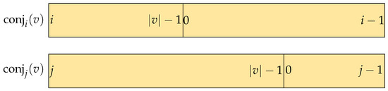
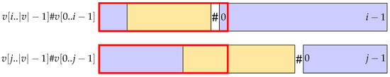
We refer to ${\mathrm{conj}}_{n-3}\left(F_{2k}^{♭}\right)$ from Lemma 3 as v here if only $0\le i,j\le f_{2k}-1$. The conjugates of v with index i and j are ${\mathrm{conj}}_i\left(v\right)$, ${\mathrm{conj}}_j\left(v\right)$, respectively. Also, we set the lexicographic order between two conjugates as ${\mathrm{conj}}_i\left(v\right)<{\mathrm{conj}}_j\left(v\right)$; thus, $v[i..|v|-1]v[0..i-1]<v[j..|v|-1]v[0..j-1]$. We prove this separately in two cases, where Figure 1 sketches the setting.

Figure 1. Sketch of the setting ${\mathrm{conj}}_i\left(v\right)<{\mathrm{conj}}_j\left(v\right)$ considered in the proof of Lemma 4.

Case 1:

  |lcp(${\mathrm{conj}}_i\left(v\right),{\mathrm{conj}}_j\left(v\right)$)| < min($\left|v\right|-i+1,\left|v\right|-j+1$);

Case 2:

  |lcp(${\mathrm{conj}}_i\left(v\right),{\mathrm{conj}}_j\left(v\right)$)| > min($\left|v\right|-i+1,\left|v\right|-j+1$).

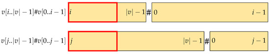
The red rectangle in Figure 2 is an example of a common prefix of ${\mathrm{conj}}_i\left(v\right)$ and $con{j}_j\left(v\right)$. In Case 1, it is ${\mathrm{conj}}_i\left(v\right)<{\mathrm{conj}}_j\left(v\right)$, meaning that the character of ${\mathrm{conj}}_i\left(v\right)$ in position |lcp(${\mathrm{conj}}_i\left(v\right),{\mathrm{conj}}_j\left(v\right)$)|+1 is smaller than in the one in the same position in ${\mathrm{conj}}_j\left(v\right)$. Thus, inserting # in position $\left|v\right|$ does not change the lexicographic order between ${\mathrm{conj}}_i\left(v\right)$ and ${\mathrm{conj}}_j\left(v\right)$. The order is preserved.

Figure 2. Illustration of the first case in Lemma 4. Inserting # does not change the lexicographic order between ${\mathrm{conj}}_i\left(v\right)$ and ${\mathrm{conj}}_j\left(v\right)$.

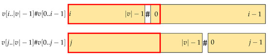
The red rectangle in Figure 3 depicting the longest common prefix of the two strings in question is longer than |lcp(${\mathrm{conj}}_i\left(v\right),{\mathrm{conj}}_j\left(v\right)$)|. In Case 2, it must be $i>j$, which means $\left|v\right[i..\left|v\right|-1\left]\right|<\left|v\right[j..\left|v\right|-1\left]\right|$. When it is $i<j$, then $\left|v\right[j..\left|v\right|-1\left]\right|<\left|v\right[i..\left|v\right|-1\left]\right|$, meaning that # appears first in ${\mathrm{conj}}_j\left(v\right)$. As a result, ${\mathrm{conj}}_j\left(v\right)<{\mathrm{conj}}_i\left(v\right)$, which contradicts ${\mathrm{conj}}_i\left(v\right)<{\mathrm{conj}}_j\left(v\right)$. Thus, in Case 2, we only consider when it is $i>j$, as illustrated in Figure 3.

Figure 3. Illustration of the second case in Lemma 4.

Furthermore, we distinguish the second case between two subcases: We let u be unique circular factor which is smaller than all the other circular factors having the same length in v.

Case 2 (a):

  when u is a prefix of $v[i..|v|-1]$;

Case 2 (b):

  when $v[0..i-1]$ is a prefix of u.

When it is Case 2 (a), u appears only in the prefix of $v[0..i-1]$. Thus, the first difference between ${\mathrm{conj}}_i\left(v\right)$ and ${\mathrm{conj}}_j\left(v\right)$ lies within the unique occurrence of u. The situation is depicted at Figure 4. After inserting the #, ${\mathrm{conj}}_i\left(v\right)$ becomes $v[i..|v|-1]\#v[0..i-1]$, creating factor $\#u$ at position $\left|v\right|-i+1$, which is not only unique but also smallest among other factors of length $|\#u|$ in v. Any factor that appears in the same position in $v[j..|v|-1]\#u$ is greater than $\#u$. Thus, the order is preserved.

Figure 4. Illustration of Case 2 (a) in Lemma 4. Inserting # in does not affect lexicographic order between ${\mathrm{conj}}_i\left(v\right)$ and ${\mathrm{conj}}_j\left(v\right)$.

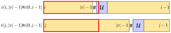
In Case 2 (a), u is the smallest prefix which appears only once in $v[0..i-1]$. v is a Lyndon word; thus, $v[0..i-1]$, it is also the smallest factor in v. However, in Case 2 (b), u is longer than $v[0..i-1]$. We sketch the situation in Figure 5, where we visualize u with a purple rectangle. Therefore, $v[0..i-1]$ must appear more than twice in u. If $v[0..i-1]$ appears only once, u is analogous with $v[0..i-1]$. Also, from ${\mathrm{conj}}_i\left(v\right)\ne {\mathrm{conj}}_j\left(v\right)$, there must be a difference in $v[0..i-1]$. Moreover, since v is primitive, v cannot be expressed in the form $Z^k$ for word Z and a integer $k\ge 2$. The first distinct character between ${\mathrm{conj}}_i\left(v\right)\mathrm{and}{\mathrm{conj}}_j\left(v\right)$ is within ${\mathrm{conj}}_i\left(v\right)\left[\right|v|-i+1..|v|-1]$. We assume otherwise that there is no mismatching character pair with $v[0..i-1]$ and the prefix of ${\mathrm{conj}}_i\left(v\right)$, which is $v[i..2i-1]$. Since $v[0..i-1]=v[i..[2i-1]$, ${\mathrm{conj}}_i\left(v\right)$ also has a smallest prefix and it contradicts with v, which is one and only Lyndon word. Moreover, ${\mathrm{conj}}_i\left(v\right)$ becomes $v[0..i-1]v[i..2i-1]\dots =v{[0..i-1]}^2\dots$, thus contradicting its primitivity.

Figure 5. Illustration of Case 2 (b) in Lemma 4.

In this way, after inserting a #, the analogous behavior of Case 2 (a) is observed.

The order of original conjugates of v is preserved with respect to the original BWT according to the cases above. Thus, the only difference in inserting # in v occurs in conjugates of $\#v$ and $v\#$. On the one hand, we observe that $\#v$ is now the smallest among all conjugates of $\mathcal{M}(\#v)$, and it ends with the last character of v. On the other hand, $v\#$ becomes the second smallest conjugate and ends with #. Hence, we have BWT($\#v$) = $\mathrm{BWT}\left(v\right)\left[0\right]·\#·\mathrm{BWT}\left(v\right)[1..|v|-1]$, which concludes the proof. □

Theorem 1.

We let $F_{2k}$ be the Fibonacci word of even order $2k>4$, and $f_{2k}=\left|F_{2k}\right|$. We let $F_{2k}^{♭}$ be the word that results from substituting a $\mathtt{b}$ by a # at position $f_{2k}-1$. Then, $r(F_{2k}^{♭}\#)=2k+2$.

Proof. 

We let $S=F_{2k}^{♭}\#$. From Lemma 2, $r\left(F_{2k}^{♭}\right)=2k$. And by Lemma 3, we know that ${\mathrm{conj}}_{n-3}\left(F_{2k}^{♭}\right)$ is the smallest conjugate among $\mathcal{M}\left(F_{2k}^{♭}\right)$. By Lemma 4, we have $2k\le r(\#{\mathrm{conj}}_{n-3}\left(F_{2k}^{♭}\right))\le 2k+2$. More precisely, it is $2k+2$ since $\#{\mathrm{conj}}_{n-3}\left(F_{2k}^{♭}\right)$ is the smallest conjugate in $\mathcal{M}(F_{2k}^{♭}\#)$ and ${\mathrm{conj}}_{n-3}\left(F_{2k}^{♭}\right)\#$ is the second smallest conjugate. The relative order among the conjugates of $\#{\mathrm{conj}}_{n-3}\left(F_{2k}^{♭}\right)$ coincides with that of the conjugates of $F_{2k}^{♭}$, using the same argument as in the proof of Lemma 4. This means that to obtain $\mathrm{BWT}\left(S\right)$, it suffices to insert a # between the first two $\mathtt{b}$s in $BWT\left(F_{2k}^{♭}\right)$. Since $r(\#{\mathrm{conj}}_{n-3}\left(F_{2k}^{♭}\right))=r(\#F_{2k}^{♭})=r(F_{2k}^{♭}\#)$, we obtain the claim.    □

5. Additive Sensitivity of $\mathit{r}$ by $\mathsf{\Omega }\left(\sqrt{\mathit{n}}\right)$

In Section 4, we presented a word such that substituting one of its characters by #, which is strictly lexicographically smaller than all its characters, resulted in a logarithmic multiplicative increase in the number of runs r in the BWT. We now follow (Giuliani et al. [24], Section 4), who presented a family of words where a single edit can produce an additive increase of $\Theta \left(\sqrt{n}\right)$ in r. Like before, we want to study the sensitivity when introducing a new character (#) in Section 5.1 or additionally when inverting the order of the alphabet in Section 5.2.

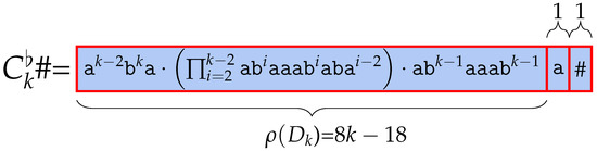
Definition 1.

For any $k>5$, we let $P_k={\mathtt{ab}}^k\mathtt{aa}$ and $E_k={\mathtt{ab}}^k{\mathtt{aba}}^{k-2}$ for all $i\in [2..k-1]$, and $Q_k={\mathtt{ab}}^k\mathtt{a}$. Then,

$$W_k=\left(\prod _{i=2}^{k-1}{P}_i{E}_i\right)Q_k=\left(\prod _{i=2}^{k-1}{\mathtt{ab}}^i{\mathtt{aaab}}^i{\mathtt{aba}}^{i-2}\right){\mathtt{ab}}^k\mathtt{a}.$$

(1)

The length of these words is

$$n=\sum _{i=2}^{k-1}(3i+4)+(k+2)={\displaystyle \frac{3k^2+7k}{2}}-9.$$

(2)

Thus, $k=\Theta \left(\sqrt{n}\right)$. $W_k^{♭}$ is

$$W_k^{♭}=\left(\prod _{i=2}^{k-1}{P}_i{E}_i\right){\mathtt{ab}}^k=\left(\prod _{i=2}^{k-1}{\mathtt{ab}}^i{\mathtt{aaab}}^i{\mathtt{aba}}^{i-2}\right){\mathtt{ab}}^k.$$

(3)

We append #, which is lexicographically smaller than character $\mathtt{a}$ at the last part of $W_k^{♭}$ and name the resulting word $W_k^{♭}\#$.

Also, $W_k$, with its characters $\mathtt{a}$ and $\mathtt{b}$ swapped, is defined as $\overline{W_k}$, which is

$$\overline{W_k}=\left(\prod _{i=2}^{k-1}\overline{P_i}\overline{E_i}\right)\overline{Q_k}=\left(\prod _{i=2}^{k-1}{\mathtt{ba}}^i{\mathtt{bbba}}^i{\mathtt{bab}}^{i-2}\right){\mathtt{ba}}^k\mathtt{b}.$$

(4)

To characterize the BWT of words $W_k^{♭}\#$, $\overline{W_k}$ and $\overline{W_k^{♭}}\mathtt{c}$, we partition each of the BWT conjugates $\mathcal{M}(W_k^{♭}\#)$, $\mathcal{M}\left(\overline{W_k}\right)$, $\mathcal{M}\left(\overline{W_k^{♭}}\mathtt{c}\right)$ into distinct groups of consecutive conjugates having identical prefixes and define the subword of BWT($W_k$) corresponding to each of these prefixes.

Given $X\in {\mathsf{\Sigma }}^{*}$, we denote by $\beta (X,W_k)$ the subword of BWT$\left(W_k\right)$ corresponding to the range of contiguous conjugates prefixed by X. We omit the second parameter of $\beta (X,W_k)$ when it is clear from the context. $\beta \left(X\right)$ is the concatenation of the last characters of conjugates with prefix X. For example, when X is $\mathtt{banana}$, there are two conjugates starting with the prefix $\mathtt{an}$ which are $\mathtt{ananab}$ and $\mathtt{anaban}$; thus, $\beta$($\mathtt{an}$) of $\mathtt{banana}$ is $\mathtt{bn}$.

Lemma 5.

In Proposition 28 of [24], it is already known that $r\left(W_k\right)=6k-12$.

5.1. BWT of $W_k$ After Substituting a Character

The lemmas presented below characterize the BWT of $W_k$ after certain modifications have been applied. Rather than deriving the entire structure of the BWT from scratch, we analyze how replacing a character affects either the relative order or the final character of the conjugates of $W_k$. We let $\mathcal{M}(W_k^{♭}\#)$ be the list of lexicographically sorted conjugates of the word $W_k^{♭}\#$.

Lemma 6.

$\beta (\#,W_k^{♭}\#)=\mathtt{b}$.

Proof. 

The first conjugate in $\mathcal{M}(W_k^{♭}\#)$ is $\#P_2\cdots \mathtt{b}$. Since the lexicographic order of # is smaller than all other characters, a conjugate starting with # is smaller than every conjugate starting with $\mathtt{a}$. # can be obtained by the last character of $W_k^{♭}\#$, which is preceded by a $\mathtt{b}$. □

Lemma 7.

$\beta ({\mathtt{a}}^i\mathtt{b},W_k^{♭}\#)$ = ${\mathtt{ba}}^{k-i-2}$ for all $i\in [4..k-2]$.

Proof. 

Given integer $i\in [4..k-2]$, the conjugates of $\mathcal{M}(W_k^{♭}\#)$ starting with ${\mathtt{a}}^i\mathtt{b}$ are

$$\begin{array}{c}\hfill {\mathtt{a}}^{i-1}{P}_{i+2}\cdots \mathtt{b}<{\mathtt{a}}^{i-1}{P}_{i+3}\cdots \mathtt{a}<\cdots <{\mathtt{a}}^{i-1}{P}_{k-1}\cdots \mathtt{a}<{\mathtt{a}}^{i-1} Q_k^{♭}\#\cdots \mathtt{a}.\end{array}$$

In $\mathcal{M}(W_k^{♭}\#)$, a prefix ${\mathtt{a}}^i\mathtt{b}$ can only be obtained by concatenation of the suffix ${\mathtt{a}}^{i-2}$ of $E_i$, with the prefix $\mathtt{ab}$ of $P_{i+1}$ or the prefix of $\mathtt{ab}$ of $Q_k^{♭}\#$ if $i=k$. Note that all these conjugates end with an $\mathtt{a}$, with the exception of the conjugate starting with ${\mathtt{a}}^{i-1}{P}_{i+1}$, since this is where the unique occurrence of ${\mathtt{ba}}^{i-1}\mathtt{b}$ can be found.    □

Lemma 8.

$\beta (\mathtt{aaab},W_k^{♭}\#)={\mathtt{b}}^5{\left(\mathtt{ab}\right)}^{k-6}\mathtt{a}$.

Proof. 

The conjugates in $\mathcal{M}(W_k^{♭}\#)$ starting with $\mathtt{aaab}$ are

$$\begin{array}{cc}\hfill \mathtt{aa}{E}_2\cdots \mathtt{b}& <\mathtt{aa}{E}_3\cdots \mathtt{b}<\mathtt{aa}{E}_4\cdots \mathtt{b}<\mathtt{aa}{P}_5\cdots \mathtt{b}<\mathtt{aa}{E}_5\cdots \mathtt{b}\hfill \\ & <\mathtt{aa}{P}_6\cdots \mathtt{a}<\mathtt{aa}{E}_6\cdots \mathtt{b}<\cdots <\mathtt{aa}{P}_{k-1}\cdots \mathtt{a}<\mathtt{aa}{E}_{k-1}\cdots \mathtt{b}\hfill \\ & <\mathtt{aa} Q_k^{♭}\#\cdots \mathtt{a}.\hfill \end{array}$$

In $\mathcal{M}(W_k^{♭}\#)$, the conjugates that start with $\mathtt{aaab}$ can be obtained for all $i\in [4..k-1]$ from the concatenation of the suffix $\mathtt{aa}$ from $E_i$ with $P_{i+1}$ or with $Q_k^{♭}\#$ if $i=k$. If $i\in [2..k-1]$, concatenation of the suffix $\mathtt{aa}$ of $P_i$ with the prefix $\mathtt{ab}$ of $E_i$ also makes $\mathtt{aaab}$. Also, we can sort the conjugates with following order: ${\bigcup }_{i=2}^4\left\{\mathtt{aa}{E}_i\right\}\cup {\bigcup }_{i=5}^{k-1}\left\{\mathtt{aa}{P}_i\mathtt{aa}{E}_i\right\}\cup \{\mathtt{aa}{Q}_k^{♭}\#\}$. All conjugates of $\mathtt{aa}{E}_i$ end with a $\mathtt{b}$ and if $i\in [5..k-2]$, $\mathtt{aa}$ of $E_i$ concatenated with $P_{i+1}$ or $Q_k^{♭}\#$ if $i=j$ also ends with $\mathtt{a}$. On the other hand, $\mathtt{aa}{P}_5$ ends with $\mathtt{b}$.    □

Lemma 9.

$\beta (\mathtt{aab},W_k^{♭}\#)={\mathtt{aaba}}^{2k-8}$.

Proof. 

The conjugates in $\mathcal{M}(W_k^{♭}\#)$ starting with $\mathtt{aab}$ are

$$\begin{array}{cc}\hfill \mathtt{a}{E}_2\cdots \mathtt{a}& <\mathtt{a}{E}_3\cdots \mathtt{a}<\mathtt{a}{P}_4\cdots \mathtt{b}\hfill \\ & <\mathtt{a}{E}_4\cdots \mathtt{a}<\mathtt{a}{P}_5\cdots \mathtt{a}<\mathtt{a}{E}_5\cdots \mathtt{a}<\cdots <\mathtt{a}{P}_{k-1}\cdots \mathtt{a}<\mathtt{a}{E}_{k-1}\cdots \mathtt{a}<\mathtt{a}{Q}_k^{♭}\#\cdots \mathtt{a}.\hfill \end{array}$$

Each of the conjugates starting with $\mathtt{aaab}$ from Lemma 8 induces a conjugate starting with $\mathtt{aab}$, obtained by shifting on the left one character $\mathtt{a}$. It follows that all of these conjugates end with an $\mathtt{a}$. The other conjugates that start with $\mathtt{aab}$ are those obtained by concatenating the suffix $\mathtt{a}$ of $E_3$ with the prefix $\mathtt{ab}$ of $P_4$ which ends with $\mathtt{b}$. □

Lemma 10.

$\beta (\mathtt{ab},W_k^{♭}\#)={\mathtt{b}}^{k-2}\#{\mathtt{aba}}^{2k-6}$.

Proof. 

The conjugates in $\mathcal{M}(W_k^{♭}\#)$ starting with the prefix $\mathtt{ab}$ are

$$\begin{array}{cc}\hfill {\mathtt{aba}}^{k-3}{Q}_k^{♭}\#\cdots \mathtt{b}& <{\mathtt{aba}}^{k-4}{P}_{k-1}\cdots \mathtt{b}<\cdots <\mathtt{ab}{P}_3\cdots \mathtt{b}\hfill \\ & <P_2\cdots \#<E_2\cdots \mathtt{a}<P_3\cdots \mathtt{b}\hfill \\ & <E_3\cdots \mathtt{a}<P_4\cdots \mathtt{a}<E_4\cdots \mathtt{a}<\cdots <P_{k-1}\cdots \mathtt{a}<E_{k-1}\cdots \mathtt{a}<Q_k^{♭}\#\cdots \mathtt{a}.\hfill \end{array}$$

For all two distinct integers $i,i^{\prime }$ with $i>i^{\prime }\ge 0$, we have ${\mathtt{aba}}^i\mathtt{b}<{\mathtt{aba}}^{i^{\prime }}\mathtt{b}$. Thus, the first conjugate in the lexicographic order starting with $\mathtt{ab}$ is the one followed by the longest $\mathtt{a}$. The smallest of these conjugates can be found from the suffix ${\mathtt{aba}}^{k-3}\mathtt{b}$ of $E_{k-1}$, followed by the suffix ${\mathtt{aba}}^{i-2}\mathtt{b}$ of $E_i$ for all $2\le i\le k-2$ taken in decreasing order.

By construction of $E_i$, for all $2\le i\le k-1$, these conjugates must end in a $\mathtt{b}$. The remaining conjugates starting with $\mathtt{ab}$ are exactly those of either $P_i$ or $E_i$, for all $2\le i\le k-1$, or $Q_k^{♭}\#$. The conjugates can be obtained by shifting on the left one character $\mathtt{a}$ from the conjugates starting with $\mathtt{aab}$ from Lemma 9, with the exception of one starting with $P_3$ since it ends with a $\mathtt{b}$, and the other starting with $P_2$ which ends with #, while the other conjugates end with an $\mathtt{a}$. □

Lemma 11.

$\beta ({\mathtt{b}}^i\#,W_k^{♭}\#)=\mathtt{b}$ for all $1\le i\le k-1$.

Proof. 

The conjugate in $\mathcal{M}(W_k^{♭}\#)$ starting with ${\mathtt{b}}^i\#$ for all $1\le i\le k-1$ is ${\mathtt{b}}^i\#P_2\cdots \mathtt{b}$. This conjugate can be obtained by a suffix of $Q_k^{♭}\#$, and is always preceded by a $\mathtt{b}$.    □

Lemma 12.

$\beta (\mathtt{ba},W_k^{♭}\#)={\mathtt{a}}^{k-5}{\mathtt{bbbab}}^{k-5}{\mathtt{ab}}^{k-2}\mathtt{a}$.

Proof. 

The conjugates in $\mathcal{M}(W_k^{♭}\#)$ starting with $\mathtt{ba}$ are

$$\begin{array}{cc}\hfill {\mathtt{ba}}^{k-3}{Q}_k^{♭}\#\cdots \mathtt{a}& <{\mathtt{ba}}^{k-4}{P}_{k-1}\cdots \mathtt{a}<\cdots <{\mathtt{ba}}^3{P}_6\cdots \mathtt{a}\hfill \\ & <\mathtt{baa}{E}_2\cdots \mathtt{b}<\mathtt{baa}{E}_3\cdots \mathtt{b}<\mathtt{baa}{E}_4\cdots \mathtt{b}<\mathtt{baa}{P}_5\cdots \mathtt{a}\hfill \\ & <\mathtt{baa}{E}_5\cdots \mathtt{b}<\mathtt{baa}{E}_6\cdots \mathtt{b}<\cdots <\mathtt{baa}{E}_{k-1}\cdots \mathtt{b}<\mathtt{ba}{P}_4\cdots \mathtt{a}\hfill \\ & <{\mathtt{baba}}^{k-3}{Q}_k^{♭}\#\cdots \mathtt{b}<{\mathtt{baba}}^{k-4}{P}_{k-1}\cdots \mathtt{b}<\cdots <\mathtt{bab}{P}_3\cdots \mathtt{b}<\mathtt{babbbaa}\cdots \mathtt{a}.\hfill \end{array}$$

We have as many circular occurrences of $\mathtt{ba}$ as the number of maximal character runs of $\mathtt{b}$ in $W_k^{♭}\#$. Then, for all $2\le i\le k-1$,

Case 1:

  one run of $\mathtt{b}$ in $P_i$ and

Case 2:

  two runs in $E_i$.

For Case 1, we have one conjugate starting with $\mathtt{baa}{E}_i$ for each $i\in [2..k-1]$. Since each run of $\mathtt{b}$ within each word of $P_i$ is of length of at least 2, all conjugates in (1) end with $\mathtt{b}$. For Case 2, for all $i\in [2..k-1]$ we can distinguish between two subcases, based on where $\mathtt{ba}$ starts:

Case 2 (a):

  from the first run of $\mathtt{b}$ in $E_i$, which is ${\mathtt{baba}}^{i-2}{P}_{i+1}$ when $i\in [2..k-2]$ or ${\mathtt{baba}}^{k-3}{Q}_k^{♭}\#$ if $i=k-1$. Since $\mathtt{b}$ has at least 2 runs, conjugates with prefix (2.1) always end with $\mathtt{b}$.

Case 2 (b):

  from run ${\mathtt{ba}}^{i-3}{P}_{i+1}$ for all $i\in [2..k-2]$, and ${\mathtt{ba}}^{k-3}{Q}_k^{♭}\#$. Each conjugate of Case 2 (b) is obtained by shifting two characters to the right in each conjugate in Case 2 (a). Therefore, these conjugates end with an $\mathtt{a}$.

Observe that only for Case 2 (b) we have conjugates starting with $\mathtt{baaaa}$. Hence, the first conjugate in the lexicographic order is the one starting with ${\mathtt{ba}}^{k-3}{Q}_k^{♭}\#$, followed by those starting with ${\mathtt{ba}}^{k-4}{P}_{k-1}<{\mathtt{ba}}^{k-5}{P}_{k-2}<\cdots <\mathtt{baaa}{P}_6$.

Among the remaining conjugates, those that have the prefix $\mathtt{baaa}$ start with $\mathtt{baa}{P}_5$ from Case 2 (b) or $\mathtt{baa}{E}_i$ from Case 2 (a). Thus, we can sort them according to lexicographic order. Then, the remaining conjugates, which start with $\mathtt{baa}$, are obtained by $\mathtt{ba}{P}_3$ only. Finally, let us focus on the conjugates from Case 2 (a), which start with $\mathtt{ba}$. These conjugates are sorted according to the length of the runs of $\mathtt{a}$s following the common prefix $\mathtt{bab}$, similarly to the sorting of conjugates from Case 2 (b). The last conjugate left is the one starting with $\mathtt{b}{P}_3$ from Case 2 (b). Since $\mathtt{b}{P}_3$ is lexicographically greater than all other cases, this is the greatest conjugate of $W_k^{♭}\#$ starting with $\mathtt{ba}$ and we can conclude our claim.    □

Lemma 13.

$\beta ({\mathtt{b}}^j\mathtt{a},W_k^{♭}\#)=\mathtt{a}{\mathtt{b}}^{2k-2j-2}\mathtt{a}$ for all $2\le j\le k-2$.

Proof. 

The conjugates starting with ${\mathtt{ba}}^i$ with integer $2\le j\le k-2$ in $\mathcal{M}(W_k^{♭}\#)$ are

$$\begin{array}{cc}\hfill {\mathtt{b}}^i\mathtt{aa}{E}_i\cdots \mathtt{a}& <{\mathtt{b}}^i\mathtt{aa}{E}_{i+1}\cdots \mathtt{b}<\cdots <{\mathtt{b}}^i\mathtt{aa}{E}_{k-1}\cdots \mathtt{b}\hfill \\ & <{\mathtt{b}}^i{\mathtt{aba}}^{k-3}{Q}_k^{♭}\#\cdots \mathtt{b}<{\mathtt{b}}^i{\mathtt{aba}}^{k-4}{P}_{k-1}\cdots \mathtt{b}<\cdots <{\mathtt{b}}^i{\mathtt{aba}}^{i-1}{P}_{i+2}\cdots \mathtt{b}\hfill \\ & <{\mathtt{b}}^i{\mathtt{aba}}^{i-2}{P}_{i+1}\cdots \mathtt{a}.\hfill \end{array}$$

All runs of $\mathtt{b}$ of length at least $2\le i\le k-2$ appear in either

Case 1:

  $P_i$ or

Case 2:

  $E_i$ for all $i\le j\le k-1$.

Let us consider these two cases separately. For all $i\le j\le k-1$, the conjugate starting within $P_j$ has prefix ${\mathtt{b}}^i\mathtt{aa}{E}_j$. For all $i\le j\le k-2$, the conjugate starting within $E_j$ has prefix ${\mathtt{b}}^i{\mathtt{aba}}^{j-2}{P}_{j+1}$, and for $j=k-1$, we have the conjugate with prefix ${\mathtt{b}}^i{\mathtt{aba}}^{k-3}{Q}_k^{♭}\#$. By construction, we have all the conjugates from Case 1 sorted according to the lexicographic order of the words with respect to the length of the run by $\mathtt{b}$ obtained by $E_j$.

The conjugates covered by Case 2 are sorted according to the decreasing length of the run of $\mathtt{a}$, following the common prefix ${\mathtt{b}}^i\mathtt{ab}$. Only when the run of $\mathtt{b}$ is exactly i long, its conjugate ends with $\mathtt{a}$. Thus, the conjugates ending with an $\mathtt{a}$ are those starting with $P_i$ and $E_i$, which have prefixes ${\mathtt{b}}^i\mathtt{aa}{E}_i$ and ${\mathtt{b}}^i{\mathtt{aba}}^{i-2}{P}_{i+1}$.    □

Lemma 14.

$\beta ({\mathtt{b}}^{k-1}\mathtt{a},W_k^{♭}\#)=\mathtt{aa}$.

Proof. 

The two conjugates in $\mathcal{M}(W_k^{♭}\#)$ which start with ${\mathtt{ba}}^{k-1}\mathtt{a}$ are

$$\begin{array}{c}\hfill {\mathtt{b}}^{k-1}\mathtt{aa}{E}_{k-1}\cdots \mathtt{a}<{\mathtt{b}}^{k-1}{\mathtt{aba}}^{k-3}{Q}_k^{♭}\#\cdots \mathtt{a}.\end{array}$$

The conjugates with the prefix ${\mathtt{b}}^{k-1}\mathtt{a}$ start with $E_{k-1}$ or $Q_k^{♭}\#$. These conjugates have prefixes of ${\mathtt{b}}^{k-1}\mathtt{aa}{E}_{k-1}$ and ${\mathtt{b}}^{k-1}\mathtt{aba}{Q}_k^{♭}\#$, respectively. One can see that these conjugates taken in this order are already sorted, and both conjugates end with $\mathtt{a}$.    □

Lemma 15.

$\beta ({\mathtt{b}}^k\#,W_k^{♭}\#)=\mathtt{a}$.

Proof. 

The last conjugate in $\mathcal{M}(W_k^{♭}\#)$ is ${\mathtt{b}}^k\#P_2\cdots \mathtt{a}$. The last conjugate in lexicographic order starts with ${\mathtt{b}}^k\#P_2$, and since the run of $\mathtt{b}$ is maximal, it ends with $\mathtt{a}$, and the claim follows. □

In conclusion, we define the above theorem.

Theorem 2.

$r(W_k^{♭}\#)-r\left(W_k\right)=2k-5$ for every $k\ge 6$.

Proof. 

The BWT of the $W_b^k\#$ is BWT($W_b^k\#$) =$\beta (\#){\prod }_{i=2}^{k-1}\beta \left({\mathtt{a}}^{k-i}\mathtt{b}\right)·{\prod }_{i=1}^{k-1}\beta ({\mathtt{b}}^i\#)\beta \left({\mathtt{b}}^i\mathtt{a}\right)·\beta \left({\mathtt{b}}^k\mathtt{a}\right)$. We refer to Table 2. Moreover, $r(W_k^{♭}\#)=8k-17$ which has $2k-5$ more runs than $r\left(W_k\right)=6k-12$, cf. Lemma 5.

Table 2. Classification of the number of runs obtain in Theorem 2. The total number of runs is $8k-17$.

BWT of ${\mathit{W}}_{\mathit{k}}^{♭}\#$	Runs
$\beta (\#)=\mathtt{b}$	1
$\beta \left({\mathtt{a}}^i\mathtt{b}\right)$ = ${\mathtt{ba}}^{k-i-2}$ for all $4\le i\le k-2$	$2k-11$ but, when merged, $2k-12$
$\beta \left(\mathtt{aaab}\right)={\mathtt{b}}^5{\left(\mathtt{ab}\right)}^{k-6}\mathtt{a}$	$2k-10$ but, when merged, $2k-11$
$\beta \left(\mathtt{aab}\right)={\mathtt{aaba}}^{2k-8}$	3 but, when merged, 2
$\beta \left(\mathtt{ab}\right)={\mathtt{b}}^{k-2}\#{\mathtt{aba}}^{2k-6}$	5
$\beta ({\mathtt{b}}^i\#)=\mathtt{b}$ for all $i\in [1..k-1]$	$k-1$
$\beta \left(\mathtt{ba}\right)={\mathtt{a}}^{k-5}{\mathtt{bbbab}}^{k-5}{\mathtt{ab}}^{k-2}\mathtt{a}$	7
$\beta \left({\mathtt{b}}^j\mathtt{a}\right)=\mathtt{a}{\mathtt{b}}^{2(k-j-1)}\mathtt{a}$ for all $j\in [2..k-2]$	$3(k-3)$
$\beta \left({\mathtt{b}}^{k-1}\mathtt{a}\right)=\mathtt{aa}$	1
$\beta ({\mathtt{b}}^k\#)=\mathtt{a}$	1 but, when merged, 0

The lexicographic order of # is lower than an $\mathtt{a}$, and a conjugate starting with # is smaller than any conjugate starting with $\mathtt{a}$. Moreover, every conjugate in $\beta \left({\mathtt{a}}^i\mathtt{b}\right)$ is smaller than every one in $\beta \left({\mathtt{a}}^{i^{\prime }}\mathtt{b}\right)$, for every $1\le i^{\prime }\le i\le k-2$. In addition, every conjugate contributing a character to $\beta \left({\mathtt{b}}^j\mathtt{a}\right)$ is smaller than a conjugate contributing a character to $\beta \left({\mathtt{b}}^{j^{\prime }}\mathtt{a}\right)$ for every $1\le j\le j^{\prime }\le k-1$. And with a conjugate starting with $b^i\#$, the number is smaller than that of ${\mathtt{b}}^i\mathtt{a}$. Since we considered all the disjoint ranges of conjugates of $W_k^{♭}\#$ based on their common prefix, the word BWT($W_k^{♭}\#$) is $\beta (\#){\prod }_{i=2}^{k-1}\beta \left({\mathtt{a}}^{k-i}\mathtt{b}\right)·{\prod }_{i=1}^{k-1}\beta ({\mathtt{b}}^i\#)\beta \left({\mathtt{b}}^i\mathtt{a}\right)·\beta \left({\mathtt{b}}^k\mathtt{a}\right)$. With the structure of BWT($W_k^{♭}\#$), we can derive its number of runs. The words $\beta (\#)$ and ${\prod }_{i=2}^{k-4}\beta \left({\mathtt{a}}^{k-i}\mathtt{b}\right)$ have $2(k-6)$ runs: we start with 1 run from $\beta (\#)$ = $\mathtt{b}$ which is merged by $\beta \left({\mathtt{a}}^{k-2}\mathtt{b}\right)\beta \left({\mathtt{a}}^{k-3}\mathtt{b}\right)$ = $\mathtt{bba}$. And concatenating them $\beta \left({\mathtt{a}}^i\mathtt{b}\right)$ up to $\beta \left({\mathtt{a}}^4\mathtt{b}\right)$ adds 2 new runs each. $\beta$$\left(\mathtt{aaab}\right)$, $\beta$($\mathtt{aab}$), $\beta$($\mathtt{ab}$) have $2(k-5)$, 3, 5 runs, respectively. However, the boundaries between $\beta$$\left(\mathtt{aaab}\right)$ and $\beta$($\mathtt{aab}$) are merged by an $\mathtt{a}$; therefore, $\beta \left(\mathtt{aab}\right)$ has 2 runs. $\beta (\mathtt{b}\#)$ has 1 run, followed by $\beta \left(\mathtt{ba}\right)$ which makes 7 runs. Then, $\beta ({\mathtt{b}}^i\#)$ and $\beta$(${\mathtt{b}}^i\mathtt{a}$) repeat, making 1 and 3 runs until $i=k-2$ thus makes $4(k-3)$ runs. $\beta ({\mathtt{b}}^{k-1}\#)$ adds 1 run. Also, $\beta \left({\mathtt{b}}^{k-1}\mathtt{a}\right)$ adds 1 run and is the last run since $\beta ({\mathtt{b}}^k\#)$ does not add new runs, since it consists only of a $\mathtt{a}$ that merges with the previous one. Altogether, we have $2(k-6)+2(k-5)+2+5+1+7+4(k-3)+1+1=8k-17$, and the claim holds. The main difference in the runs of $W_k^{♭}\#$ and $W_k$ occurs from the prefix beginning with ${\mathtt{b}}^i\#$ that concatenates with ${\mathtt{b}}^i\mathtt{a}$, repeating $\mathtt{baba}$ for $i\in [2..k-1]$, while $W_k$ repeats only $\mathtt{ba}$. Thus, it makes additive runs of $2k-5=\Theta \left(k\right)=\Theta \left(\sqrt{n}\right)$.

Table 3, Table 4, Table 5, Table 6 and , Table 7 $\mathcal{M}(W_k^{♭}\#)$. The first column partitions conjugates by common prefixes and names the common prefix shared by all conjugates in a partition. The second column shows the remaining part of the respective conjugate followed by the prefix of its partition. The remaining part of a conjugate decides its relative order inside its partition. The BWT column shows the last character of each conjugate. □

Table 3. Lexicographically sorted conjugates of $W_k^{♭}\#$ studied in Theorem 2, Part 1.

Prefix	Remaining Part	BWT
#	$P_2$	$\mathtt{b}$
${\mathtt{a}}^{k-2}\mathtt{b}$	${\mathtt{b}}^{k-1}\#$	$\mathtt{b}$
${\mathtt{a}}^{k-3}\mathtt{b}$	${\mathtt{b}}^{k-2}\mathtt{aa}$	$\mathtt{b}$
	${\mathtt{b}}^{k-1}\#$	$\mathtt{a}$
${\mathtt{a}}^{k-4}\mathtt{b}$	${\mathtt{b}}^{k-3}\mathtt{aa}$	$\mathtt{b}$
	${\mathtt{b}}^{k-2}\mathtt{aa}$	$\mathtt{a}$
	${\mathtt{b}}^{k-1}\#$	$\mathtt{a}$
...	...	...

Table 4. Lexicographically sorted conjugates of $W_k^{♭}\#$ studied in Theorem 2, Part 2.

Prefix	Remaining Part	BWT
${\mathtt{a}}^3\mathtt{b}$	$\mathtt{bab}$	$\mathtt{b}$
	$\mathtt{bbaba}$	$\mathtt{b}$
	$\mathtt{bbbabaa}$	$\mathtt{b}$
	${\mathtt{b}}^4\mathtt{aa}$	$\mathtt{b}$
	${\mathtt{b}}^4{\mathtt{aba}}^3$	$\mathtt{b}$
	${\mathtt{b}}^5\mathtt{aa}$	$\mathtt{a}$
	${\mathtt{b}}^5{\mathtt{aba}}^4$	$\mathtt{b}$
	${\mathtt{b}}^6\mathtt{aa}$	$\mathtt{a}$
	${\mathtt{b}}^6{\mathtt{aba}}^5$	$\mathtt{b}$
	...	...
	${\mathtt{b}}^{k-2}\mathtt{aa}$	$\mathtt{a}$
	${\mathtt{b}}^{k-2}{\mathtt{aba}}^{k-3}$	$\mathtt{b}$
	${\mathtt{b}}^{k-1}\#$	$\mathtt{a}$
${\mathtt{a}}^2\mathtt{b}$	$\mathtt{bab}$	$\mathtt{a}$
	$\mathtt{bbaba}$	$\mathtt{a}$
	$\mathtt{bbbaa}$	$\mathtt{b}$
	$\mathtt{bbbabaa}$	$\mathtt{a}$
	${\mathtt{b}}^4\mathtt{aa}$	$\mathtt{a}$
	${\mathtt{b}}^4{\mathtt{aba}}^3$	$\mathtt{a}$
	...	...
	${\mathtt{b}}^{k-2}\mathtt{aa}$	$\mathtt{a}$
	${\mathtt{b}}^{k-2}{\mathtt{aba}}^{k-3}$	$\mathtt{a}$
	${\mathtt{b}}^{k-1}\#$	$\mathtt{a}$

Table 5. Lexicographically sorted conjugates of $W_k^{♭}\#$ studied in Theorem 2, Part 3.

Prefix	Remaining Part	BWT
$\mathtt{ab}$	${\mathtt{a}}^{k-3}{Q}_k^{♭}\#$	$\mathtt{b}$
	${\mathtt{a}}^{k-4}{P}_{k-1}$	$\mathtt{b}$
	...	...
	$P_3$	$\mathtt{b}$
	$\mathtt{baa}$	#
	$\mathtt{bab}$	$\mathtt{a}$
	$\mathtt{bbaa}$	$\mathtt{b}$
	$\mathtt{bbaba}$	$\mathtt{a}$
	${\mathtt{b}}^3\mathtt{aa}$	$\mathtt{a}$
	${\mathtt{b}}^3{\mathtt{aba}}^2$	$\mathtt{a}$
	...	...
	${\mathtt{b}}^{k-2}\mathtt{aa}$	$\mathtt{a}$
	${\mathtt{b}}^{k-2}{\mathtt{aba}}^{k-3}$	$\mathtt{a}$
	${\mathtt{b}}^{k-1}\#$	$\mathtt{a}$
$\mathtt{b}\#$	$P_2$	$\mathtt{b}$
$\mathtt{ba}$	${\mathtt{a}}^{k-4}{Q}_k^{♭}\#$	$\mathtt{a}$
	${\mathtt{a}}^{k-5}{P}_{k-1}$	$\mathtt{a}$
	...	...
	${\mathtt{a}}^2{P}_6$	$\mathtt{a}$
	${\mathtt{b}}^2\mathtt{ab}$	$\mathtt{b}$
	${\mathtt{b}}^3\mathtt{aba}$	$\mathtt{b}$
	${\mathtt{b}}^4\mathtt{abaa}$	$\mathtt{b}$
	${\mathtt{aab}}^5\mathtt{aa}$	$\mathtt{a}$
	${\mathtt{aab}}^5{\mathtt{aba}}^3$	b
	...	...
	${\mathtt{aab}}^{k-1}{\mathtt{aba}}^{k-3}$	$\mathtt{b}$
	$P_4$	$\mathtt{a}$
	$\mathtt{b}{P}_3$	$\mathtt{b}$
	...	...
	${\mathtt{ba}}^{k-3}{Q}_k^{♭}\#$	$\mathtt{b}$
	${\mathtt{b}}^3\mathtt{aa}$	$\mathtt{a}$

Table 6. Lexicographically sorted conjugates of $W_k^{♭}\#$ studied in Theorem 2, Part 4.

Prefix	Remaining Part	BWT
$\mathtt{bb}\#$	$P_2$	$\mathtt{b}$
${\mathtt{b}}^2\mathtt{a}$	${\mathtt{aab}}^2\mathtt{ab}$	$\mathtt{a}$
	${\mathtt{aab}}^3\mathtt{aba}$	$\mathtt{b}$
	...	...
	${\mathtt{aab}}^{k-1}{\mathtt{aba}}^{k-3}$	$\mathtt{b}$
	${\mathtt{ba}}^{k-3}{Q}_k^{♭}\#$	$\mathtt{b}$
	...	...
	$\mathtt{ba}{P}_4$	$\mathtt{b}$
	$\mathtt{b}{P}_3$	a
$\mathtt{bbb}\#$	$P_2$	$\mathtt{b}$
${\mathtt{b}}^3\mathtt{a}$	${\mathtt{aab}}^3\mathtt{aba}$	$\mathtt{a}$
	${\mathtt{aab}}^4\mathtt{abaa}$	$\mathtt{b}$
	...	...
	${\mathtt{aab}}^{k-1}{\mathtt{aba}}^{k-3}$	$\mathtt{b}$
	${\mathtt{ba}}^{k-3}{Q}_k^{♭}\#$	$\mathtt{b}$
	...	...
	$\mathtt{baa}{P}_5$	$\mathtt{b}$
	$\mathtt{ba}{P}_4$	$\mathtt{a}$
$\mathtt{bbbb}\#$	$P_2$	$\mathtt{b}$
...	...	...

Table 7. Lexicographically sorted conjugates of $W_k^{♭}\#$ studied in Theorem 2, Part 5.

Prefix	Remaining Part	BWT
${\mathtt{b}}^{k-2}\#$	$P_2$	$\mathtt{b}$
${\mathtt{b}}^{k-2}\mathtt{a}$	${\mathtt{aab}}^{k-2}{\mathtt{aba}}^{k-4}$	$\mathtt{a}$
	${\mathtt{aab}}^{k-1}{\mathtt{aba}}^{k-3}$	$\mathtt{b}$
	${\mathtt{ba}}^{k-3}{Q}_k^{♭}\#$	$\mathtt{b}$
	${\mathtt{ba}}^{k-4}{P}_{k-1}$	$\mathtt{a}$
${\mathtt{b}}^{k-1}\#$	$P_2$	$\mathtt{b}$
${\mathtt{b}}^{k-2}\mathtt{a}$	${\mathtt{aab}}^{k-1}{\mathtt{aba}}^{k-3}$	$\mathtt{a}$
	${\mathtt{ba}}^{k-3}{Q}_k^{♭}\#$	$\mathtt{a}$
${\mathtt{b}}^k\#$	$P_2$	$\mathtt{a}$

5.2. BWT of $\overline{W_k}$ After Substituting a Character

In this subsection, we consider the word $\overline{W_k}=\left({\prod }_{i=2}^{k-1}\overline{P_i}\overline{E_i}\right)\overline{Q_k}=\left({\prod }_{i=2}^{k-1}{\mathtt{ba}}^i{\mathtt{bbba}}^i{\mathtt{bab}}^{i-2}\right){\mathtt{ba}}^i\mathtt{b}$, where we swapped $\mathtt{a}$ with $\mathtt{b}$ in $W_k$. The following series of lemmas characterize the subword of BWT($\overline{W_k}$) using $\mathcal{M}\left(\overline{W_k}\right)$ for each range we consider.

Lemma 16.

$\beta ({\mathtt{a}}^k\mathtt{b},\overline{W_k})=\mathtt{b}$.

Proof. 

The first conjugate in $\mathcal{M}\left(\overline{W_k}\right)$ is ${\mathtt{a}}^k\mathtt{b}\cdots \mathtt{b}.$ The first conjugate in lexicographic order must start with the longest run of $\mathtt{a}$s. By the definition of $\overline{W_k}$, the longest run of $\mathtt{a}$ has length k, which is obtained by ${\mathtt{a}}^k$ of $\overline{Q_k}$, which is preceded by a $\mathtt{b}$.    □

Lemma 17.

$\beta ({\mathtt{a}}^i\mathtt{b},\overline{W_k})={\mathtt{ba}}^{2k-2i-1}\mathtt{b}$ for all $i\in [2..k-1]$.

Proof. 

With integer $i\in [2..k-1]$, the conjugates starting with ${\mathtt{a}}^i\mathtt{b}$ in $\mathcal{M}\left(\overline{W_k}\right)$ are

$$\begin{array}{cc}\hfill {\mathtt{a}}^i{\mathtt{bab}}^{i-2}\cdots \mathtt{b}& <{\mathtt{a}}^i{\mathtt{bab}}^{i-1}\cdots \mathtt{a}<\cdots <{\mathtt{a}}^i{\mathtt{bab}}^{k-3}\cdots \mathtt{a}<{\mathtt{a}}^i\mathtt{b}\overline{P_2}\cdots \mathtt{a}\hfill \\ & <{\mathtt{a}}^i{\mathtt{bbba}}^{k-1}\cdots \mathtt{a}<\cdots <{\mathtt{a}}^i{\mathtt{bbba}}^{i+1}\cdots \mathtt{a}\hfill \\ & <{\mathtt{a}}^i{\mathtt{bbba}}^i\cdots \mathtt{b}.\hfill \end{array}$$

For all $i\in [2..k-1]$, the factor of ${\mathtt{a}}^i\mathtt{b}$ can only be obtained for all $j\in [i..k-1]$, from ${\mathtt{a}}^i{\mathtt{bab}}^{j-2}$ from $\overline{E_j}$, or ${\mathtt{a}}^i\mathtt{bb}$ from $\overline{P_j}$, and if $j=k$, ${\mathtt{a}}^i\mathtt{b}$ from $\overline{Q_k}$. We can sort the conjugate according to the lexicographic order. Note that all these conjugates end with $\mathtt{b}$, with the exception of the conjugate starting with ${\mathtt{a}}^i\mathtt{b}$ obtained by $\overline{E_i}$ and $\overline{P_i}$ ending with $\mathtt{b}$.    □

Lemma 18.

$\beta (\mathtt{ab},\overline{W_k})={\mathtt{ba}}^{k-2}{\mathtt{baa}}^{k-5}{\mathtt{baaab}}^{k-5}$.

Proof. 

In $\mathcal{M}\left(\overline{W_k}\right)$, the conjugates starting with $\mathtt{ab}$ are

$$\begin{array}{cc}\hfill \mathtt{abaaabb}\overline{E_2}\cdots \mathtt{b}& <\mathtt{aba}\overline{P_3}\cdots \mathtt{a}<\mathtt{abab}\overline{P_4}\cdots \mathtt{a}<\cdots <{\mathtt{abab}}^{k-3}\overline{Q_k}\cdots \mathtt{a}\hfill \\ & <\mathtt{ab}\overline{P_4}\cdots \mathtt{b}<\mathtt{ab}\overline{P_2}\cdots \mathtt{a}<\mathtt{abb}\overline{E_{k-1}}\cdots \mathtt{a}<\cdots <\mathtt{abb}\overline{E_5}\cdots \mathtt{a}\hfill \\ & <\mathtt{abb}\overline{P_5}<\mathtt{abb}\overline{E_4}\cdots \mathtt{a}<\mathtt{abb}\overline{E_3}\cdots \mathtt{a}<\mathtt{abb}\overline{E_2}\cdots \mathtt{a}\hfill \\ & <\mathtt{abbb}\overline{P_6}\cdots \mathtt{b}<\cdots <{\mathtt{ab}}^{k-3}\overline{Q_k}\cdots \mathtt{b}.\hfill \end{array}$$

We have as many circular occurrences of $\mathtt{ab}$ as the number of maximal (circular) runs of $\mathtt{b}$ in $\overline{W_k}$. Then, for all $i\in [2..k-1]$, we have three cases.

Case 1:

  one run of $\mathtt{ab}$ in $\overline{P_i}$,

Case 2:

  two runs in $\mathtt{ab}$ in $\overline{E_i}$,

Case 3:

  one run $\mathtt{ab}$ in $\overline{Q_k}$.

For Case 1, we have one conjugate starting with $\mathtt{abb}\overline{E_i}$, for each $i\in [2..k-1]$. Since each run of $\mathtt{a}$ within each word of $\overline{P_i}$ is of length at least 2, all conjugates in Case 1 end in $\mathtt{a}$. For Case 2, for all $i\in [2..k-1]$, we can distinguish between two sub-cases based on where $\mathtt{ab}$ starts.

Case 2 (a):

  from the first run of $\mathtt{a}$ in $\overline{E_i}$, starting with ${\mathtt{abab}}^{i-2}\overline{P_{i+1}}$, if $i\in [2..k-2]$, or ${\mathtt{abab}}^{k-3}\overline{Q_k}$,

Case 2 (b):

  from the second run in $\overline{E_i}$, starting with ${\mathtt{ab}}^{i-2}\overline{P_{i+1}}$, if $i\in [2..k-2]$, or ${\mathtt{ab}}^{k-3}\overline{Q_k}$.

Similarly to Case 1, each conjugate for Case 2 (a), ends with $\mathtt{a}$. Each conjugate in Case 2 (b) is obtained by shifting two characters on the right in each conjugate in Case 2 (a). Therefore, all these conjugates end with $\mathtt{b}$.

For Case 3, the conjugate starting with $\mathtt{ab}$ in $\overline{Q_k}$ has $\mathtt{ab}\overline{P_2}$ as a prefix and is preceded by $\mathtt{a}$. Observe that only for Case 2 (b), we have one conjugate that starts with $\mathtt{abaaa}$ obtained by $\mathtt{a}\overline{P_3}$ and it is the first conjugate in the lexicographic order of $\overline{W_k}$. Then, the conjugates start with $\mathtt{abab}$ followed by $\mathtt{aba}\overline{P_3}<\mathtt{abab}\overline{P_4}<\cdots <{\mathtt{abab}}^{k-3}\overline{Q_k}$ from Case 2 (a).

Among the remaining conjugates, those with the prefix $\mathtt{abb}$ start with $\mathtt{ab}\overline{P_4}$ from Case 2 (b) or $\mathtt{ab}\overline{P_2}$ from Case 3. Then, among the left conjugates, the conjugate with the prefix $\mathtt{abbb}$ from Case 2 (a), for all $i\in [2..k-1]$, or $\mathtt{abb}\overline{P_5}$ from Case 2 (b) follows. The last remaining conjugates have the prefix ${\mathtt{ab}}^{i-2}$ for $i\in [6..k-1]$ or ${\mathtt{ab}}^{k-3}\overline{Q_k}$, which can be obtained by Case 2 (b). Since ${\mathtt{ab}}^{k-3}\overline{Q_k}$ is greater than all other conjugates, it is the greatest conjugate of $\overline{W_k}$ starting with $\mathtt{ab}$ and we conclude this proof. □

Lemma 19.

$\beta (\mathtt{ba},\overline{W_k})={\mathtt{bb}}^{2k-8}{\mathtt{babba}}^{k-2}$.

Proof. 

The conjugates in $\mathcal{M}\left(\overline{W_k}\right)$ that start with $\mathtt{ba}$ are

$$\begin{array}{cc}\hfill {\mathtt{ba}}^k\mathtt{b}\overline{P_2}\cdots \mathtt{b}& <{\mathtt{ba}}^{k-1}{\mathtt{ab}}^{k-3}\overline{Q_k}\cdots \mathtt{b}<{\mathtt{ba}}^{k-1}\mathtt{bb}\overline{E_{k-1}}\cdots \mathtt{b}<{\mathtt{ba}}^{k-2}{\mathtt{bab}}^{k-4}\overline{P_{k-1}}\cdots \mathtt{b}\hfill \\ & <{\mathtt{ba}}^{k-2}\mathtt{bb}\overline{E_{k-2}}\cdots \mathtt{b}<\cdots <{\mathtt{ba}}^4\mathtt{babb}\overline{P_5}\cdots \mathtt{b}<{\mathtt{ba}}^4\mathtt{bb}\overline{E_4}\cdots \mathtt{b}\hfill \\ & <\mathtt{baaabab}\overline{P_4}\cdots \mathtt{b}<\mathtt{baaabb}\overline{E_3}\cdots \mathtt{a}<\mathtt{baaba}\overline{P_3}\cdots \mathtt{b}<\mathtt{baabb}\overline{E_2}\cdots \mathtt{b}\hfill \\ & <\mathtt{ba}\overline{P_3}\cdots \mathtt{a}<\mathtt{bab}\overline{P_4}\cdots \mathtt{a}<\cdots <{\mathtt{bab}}^{k-3}\overline{Q_k}\cdots \mathtt{a}.\hfill \end{array}$$

For integer i, we can see that ${\mathtt{ba}}^i{\mathtt{bab}}^{i-2}$ is lexicographically smaller than ${\mathtt{ba}}^i\mathtt{bb}$. Thus, the first conjugate in lexicographic order starting with $\mathtt{ba}$ is the one followed by the longest run of $\mathtt{a}$, and it can be found by ${\mathtt{ba}}^k\mathtt{b}$ of $\overline{Q_k}$, followed by conjugates starting with ${\mathtt{ba}}^i{\mathtt{bab}}^{i-2}$ of $\overline{E_i}$ and ${\mathtt{ba}}^i\mathtt{bb}$ of $\overline{P_i}$ for all $i\in [2..k-1]$ taken in decreasing order. By construction of $\overline{E_i}$, for $i\in [2..k-1]$, these conjugates must end with a $\mathtt{b}$. Otherwise, for $\overline{P_i}$, conjugates also end with $\mathtt{b}$, with the exception of a conjugate starting with $\overline{P_3}$, since it is preceded by an $\mathtt{a}$ from $\overline{P_2}$. The remaining conjugates starting with $\mathtt{ba}$ are exactly those conjugates that have the prefix of the suffix ${\mathtt{bab}}^{i-2}\overline{P_{i+1}}$ if $i\in [2..k-2]$ or ${\mathtt{bab}}^{k-3}\overline{Q_k}$. All of these conjugates end with $\mathtt{a}$, since they are preceded by $\mathtt{a}$.    □

Lemma 20.

$\beta (\mathtt{bba},\overline{W_k})={\mathtt{b}}^{2k-8}\mathtt{abba}$.

Proof. 

The conjugates starting with $\mathtt{bba}$ in $\mathcal{M}\left(\overline{W_k}\right)$ are

$$\begin{array}{cc}\hfill \mathtt{b}\overline{Q_k}\cdots \mathtt{b}& <\mathtt{b}\overline{E_{k-1}}\cdots \mathtt{b}<\mathtt{b}\overline{P_{k-1}}\cdots \mathtt{b}<\cdots <\mathtt{b}\overline{E_5}\cdots \mathtt{b}<\mathtt{b}\overline{P_5}\cdots \mathtt{b}<\mathtt{b}\overline{E_4}\cdots \mathtt{b}\hfill \\ & <\mathtt{b}\overline{P_4}\cdots \mathtt{a}<\mathtt{b}\overline{E_3}\cdots \mathtt{b}<\mathtt{b}\overline{E_2}\cdots \mathtt{b}<\mathtt{b}\overline{P_2}\cdots \mathtt{a}.\hfill \end{array}$$

These conjugates are obtained by following four cases.

Case 1:

  concatenating suffix $\mathtt{b}$ of $\overline{P_j}$ with $\overline{E_j}$ for all $j\in [2..k-1]$,

Case 2:

  concatenating suffix $\mathtt{b}$ of $\overline{E_j}$ with $\overline{P_{j+1}}$ for all $j\in [3..k-2]$,

Case 3:

  concatenating suffix $\mathtt{b}$ of $\overline{E_{k-1}}$ with $\overline{Q_k}$,

Case 4:

  concatenating suffix $\mathtt{b}$ of $\overline{Q_k}$ with $\overline{P_2}$.

The first conjugate in lexicographic order starting with $\mathtt{bba}$ is the one followed by the longest run of $\mathtt{a}$. The smallest of these conjugates can be found by Case 3, concatenation of the suffix $\mathtt{b}$ of $\overline{E_{k-1}}$ with $\overline{Q_k}$. We can directly observe that ${\mathtt{bba}}^j{\mathtt{bab}}^{j-2}<{\mathtt{bba}}^j\mathtt{bb}$ holds for every integer $j\ge 0$. Thus, the next conjugate will have the prefix $\mathtt{b}\overline{E_j}$ from Case 1 and $\mathtt{b}\overline{P_j}$ from Case 2 repeating in decreasing order. Since $\mathtt{b}\overline{E_j}$ of Case 1 and $\mathtt{b}\overline{Q_k}$ of Case 3 is preceded by a $\mathtt{b}$, those end with a $\mathtt{b}$. On the other hand, $\mathtt{b}\overline{P_{j+1}}$ precedes $\mathtt{b}$ for all $j\in [4..k-2]$ until $\mathtt{b}\overline{P_4}$ appears since it precedes an $\mathtt{a}$. Lastly, conjugates with the prefix $\mathtt{bbaaa}$ and $\mathtt{bbaa}$ by Case 1 end with a $\mathtt{b}$. The greatest lexicographic conjugate is from Case 4 as it has the smallest runs of $\mathtt{a}$ which is two and ends with $\mathtt{a}$.

We can sort all of these conjugates according to the order of the words in

$$\left\{\mathtt{b}\overline{Q_k}\right\}\bigcup _{j=4}^{k-1}\left\{\mathtt{b}\overline{E_j}\mathtt{b}\overline{P_j}\right\}\cup \bigcup _{j^{\prime }=2}^3\left\{\overline{E_{j^{\prime }}}\right\}\cup \left\{\mathtt{b}\overline{P_2}\right\}.$$

□

Lemma 21.

$\beta (\mathtt{bbba},\overline{W_k})=\mathtt{b}{\left(\mathtt{ab}\right)}^{k-6}{\mathtt{a}}^5$.

Proof. 

The conjugates in $\mathcal{M}\left(\overline{W_k}\right)$ starting with $\mathtt{bbba}$ are

$$\begin{array}{cc}\hfill \mathtt{bb}\overline{Q_k}\cdots \mathtt{b}& <\mathtt{bb}\overline{E_{k-1}}\cdots \mathtt{a}<\mathtt{bb}\overline{P_{k-1}}\cdots \mathtt{b}<\cdots <\mathtt{bb}\overline{E_6}\cdots \mathtt{a}<\mathtt{bb}\overline{P_6}\cdots \mathtt{b}\hfill \\ & <\mathtt{bb}\overline{E_5}\cdots \mathtt{a}<\mathtt{bb}\overline{P_5}\cdots \mathtt{a}<\mathtt{bb}\overline{E_4}\cdots \mathtt{a}<\mathtt{bb}\overline{E_3}\cdots \mathtt{a}<\mathtt{bb}\overline{E_2}\cdots \mathtt{a}.\hfill \end{array}$$

Some of the conjugates starting with $\mathtt{bbba}$ can be obtained by two cases.

Case 1:

  from the concatenation of the suffix $\mathtt{bb}$ of $\overline{E_{j-1}}$ with a prefix of $\mathtt{ba}$ of $\overline{P_j}$ for all $j\in [5..k-1]$

or $\overline{Q_k}$ if $j=k$;

Case 1:

  from the concatenation of the suffix $\mathtt{bb}$ of $\overline{P_j}$ with prefix $\mathtt{ba}$ of $\overline{E_j}$ for all $j\in [2..k-1]$.

Thus, all conjugates starting with $\mathtt{bbba}$ are sorted according to the lexicographic order of the words in $\left\{\mathtt{bb}\overline{Q_k}\right\}\cup {\bigcup }_{j=5}^{k-1}\left\{\mathtt{bb}\overline{E_j}\mathtt{bb}\overline{P_j}\right\}\cup {\bigcup }_{j=2}^4\left\{\overline{E_j}\right\}.$ All conjugates starting with $\mathtt{bb}\overline{P_j}$ for all $j\in [6..k-1]$ or $\mathtt{bb}\overline{Q_k}$ in Case 1 end with $\mathtt{b}$. Otherwise, conjugates starting with $\mathtt{bb}\overline{P_5}$ of Case 1 or $\mathtt{bb}\overline{E_j}$ for all $j\in [2..k-1]$ of Case 2 end with $\mathtt{a}$. □

Lemma 22.

$\beta ({\mathtt{b}}^j\mathtt{a},\overline{W_k})={\mathtt{b}}^{k-j-2}\mathtt{a}$ for all $j\in [4..k-2]$.

Proof. 

All runs of $\mathtt{b}$ of length of a range $j\in [4..k-3]$ appear only by concatenating suffix ${\mathtt{b}}^{j-1}$ of $E_{j+1}$ with prefix $\mathtt{ba}$ of $\overline{P_{j^{\prime }}}$ for all $j^{\prime }\in [j+2..k-1]$ in decreasing order. All of these conjugates end with a $\mathtt{b}$, with the exception of a conjugate ${\mathtt{b}}^{j-1}\overline{P_{j+2}}$ which ends with an $\mathtt{a}$ since suffix ${\mathtt{b}}^{j-1}$ precedes an $\mathtt{a}$. Hence, the last conjugate in lexicographic order starting with ${\mathtt{b}}^{k-2}\mathtt{a}$ is within ${\mathtt{b}}^{k-3}\overline{Q_k}$ and since the run of $\mathtt{b}$ is maximal it ends with $\mathtt{a}$, and the claim follows. □

The following theorem presents the shape of the BWT of $\overline{W_k}$.

Theorem 3.

For every $k\ge 6,r\left(\overline{W_k}\right)=6k-12$. cf. Table 8.

Table 8. Classification of the number of runs obtained in Theorem 3. The total number of runs is $6k-12$.

BWT of $\overline{{\mathit{W}}_{\mathit{k}}}$	Runs
$\beta \left({\mathtt{a}}^k\mathtt{b}\right)=\mathtt{b}$	1
$\beta \left({\mathtt{a}}^i\mathtt{b}\right)={\mathtt{ba}}^{2(k-1-i)+1}\mathtt{b}$ for all $i\in [2..k-1]$	$2k-3$ but, when merged, $2k-4$
$\beta \left(\mathtt{ab}\right)={\mathtt{ba}}^{k-2}{\mathtt{baa}}^{k-5}{\mathtt{baaab}}^{k-5}$	7 but, when merged, 6
$\beta \left(\mathtt{ba}\right)={\mathtt{b}}^{2k-6}{\mathtt{abba}}^{k-2}$	4 but, when merged, 3
$\beta \left(\mathtt{bba}\right)={\mathtt{b}}^{2k-8}\mathtt{abba}$	4
$\beta \left(\mathtt{bbba}\right)=\mathtt{b}{\left(\mathtt{ab}\right)}^{k-6}{\mathtt{a}}^5$	$2k-10$
$\beta \left({\mathtt{b}}^i\mathtt{a}\right)={\mathtt{b}}^{k-i-2}\mathtt{a},$ for all $i\in [4..k-2]$	$2k-12$

Proof. 

Let us put the result from Lemma 16 to Lemma 22 together. Every conjugate of contributing a character to $\beta \left({\mathtt{a}}^i\mathtt{b}\right)$ is smaller than a conjugate contributing a character to $\beta \left({\mathtt{a}}^{i^{\prime }}\mathtt{b}\right)$, for every $1\le i^{\prime }\le i\le k$. Symmetrically, every conjugate in $\beta \left({\mathtt{b}}^j\mathtt{a}\right)$ is greater than every conjugate in $\beta \left({\mathtt{b}}^{j^{\prime }}\mathtt{a}\right)$, when $1\le j^{\prime }\le j\le k-2$. Since we considered all the disjoint ranges of conjugates of $\overline{W_k}$ based on their common prefix, the word ${\prod }_{i=0}^{k-1}\beta \left({\mathtt{a}}^{k-i}\mathtt{b}\right)·{\prod }_{i=1}^{k-2}\beta \left({\mathtt{b}}^i\mathtt{a}\right)$ is the BWT of $\overline{W_k}$.

With the structure of BWT($\overline{W_k}$), we can derive its number of runs. The word ${\prod }_{i=0}^{k-1}\beta \left({\mathtt{a}}^{k-i}\mathtt{b}\right)$ has exactly $2k+3$ runs: we start with 1 run from $\beta \left({\mathtt{a}}^k\mathtt{b}\right)$ but it is merged by a $\mathtt{b}$ from $\beta \left({\mathtt{a}}^{k-1}\mathtt{b}\right)$. Then, concatenating each $\beta \left({\mathtt{a}}^{k-1}\mathtt{b}\right)$ up to $\beta \left(\mathtt{aab}\right)$ adds 3 runs each. However, the boundaries between these words merge because $\mathtt{b}$ appears continuously. Thus, each $\beta \left({\mathtt{a}}^i\mathtt{b}\right)$ for $i\in [2..k-1]$ makes 2 runs each. By counting, we observe that $\beta \left(\mathtt{ab}\right)$ runs 7 times. The remaining part of the BWT, that is, ${\prod }_{i=1}^{k-2}\beta \left({\mathtt{b}}^i\mathtt{a}\right)$ has $4k-12$ runs: the word $\beta \left(\mathtt{ba}\right)$, has 4 runs, but the first $\mathtt{b}$ merges with a $\mathtt{b}$ from $\beta \left(\mathtt{ab}\right)$, so we only charge 3 runs for this word. Then, $\beta \left(\mathtt{bba}\right)$ and $\beta \left(\mathtt{bbba}\right)$ add 4 and $1+2(k-6)+1$ runs, respectively. Finally, ${\prod }_{i=4}^{k-2}\beta \left({\mathtt{b}}^i\mathtt{a}\right)$ runs for 2 until $i=k-3$. The word $\beta \left({\mathtt{b}}^{k-2}\mathtt{a}\right)$ does not add new runs, as it consists only of an $\mathtt{a}$ that merges with the previous one. Altogether, we have $2(k-2)+7+3+4+1+2(k-6)+1+2(k-6)=6k-12$, and the claim holds. □

The following lemmas describe the BWT of $\overline{W_k}$ after applying one specific edit operation. $\overline{W_k^{♭}}\mathtt{c}$ is a word obtained by replacing the last character $\mathtt{b}$ of $\overline{W_k}$ with $\mathtt{c}$, where $\mathtt{c}$ is lexicographically larger than $\mathtt{b}$. The number of runs in the BWT of $\overline{W_k^{♭}}\mathtt{c}$ can be derived by comparing the BWT of $\overline{W_k^{♭}}\mathtt{c}$ to the BWT of $\overline{W_k}$, for which we explicitly counted the number of runs, so we omit these parts of the proof using $\mathcal{M}\left(\overline{W_k^{♭}}\mathtt{c}\right)$, which is a list of lexicographically sorted conjugates of word $\overline{W_k^{♭}}\mathtt{c}$. Substituting the last character with $\mathtt{c}$ in $\overline{W_k}$ also increases the number of runs by $\Theta \left(k\right)$.

Lemma 23.

$\beta ({\mathtt{a}}^k\mathtt{c},\overline{W_k^{♭}}\mathtt{c})=\mathtt{b}$.

Proof. 

The first conjugate in $\mathcal{M}\left(\overline{W_k^{♭}}\mathtt{c}\right)$ starts with ${\mathtt{a}}^k\mathtt{c}\cdots \mathtt{b}$. The first conjugate in lexicographic order must start with the longest run of $\mathtt{a}$. By the definition of $\overline{W_k^{♭}}\mathtt{c}$, the longest run of $\mathtt{a}$ is obtained by suffix ${\mathtt{a}}^k\mathtt{c}$ of $\overline{Q_k^{♭}}\mathtt{c}$, preceded by a $\mathtt{b}$.    □

Lemma 24.

$\beta ({\mathtt{a}}^i\mathtt{b},\overline{W_k^{♭}}\mathtt{c})={\mathtt{ba}}^{2k-2i-2}\mathtt{b}$ for all $i\in [2..k-1]$.

Proof. 

The conjugates in $\mathcal{M}\left(\overline{W_k^{♭}}\mathtt{c}\right)$ starting with the prefix ${\mathtt{a}}^i\mathtt{b}$ for $i\in [2..k-1]$ are

$$\begin{array}{cc}\hfill {\mathtt{a}}^i{\mathtt{bab}}^{i-2}\overline{P_{i+1}}\cdots \mathtt{b}& <{\mathtt{a}}^i{\mathtt{bab}}^{i-1}\overline{P_{i+2}}\cdots \mathtt{a}<\cdots <{\mathtt{a}}^i{\mathtt{bab}}^{k-4}\overline{P_{k-1}}\cdots \mathtt{a}<{\mathtt{a}}^i{\mathtt{bab}}^{k-3}\overline{Q_k^{♭}}\mathtt{c}\cdots \mathtt{a}\hfill \\ & <{\mathtt{a}}^i\mathtt{bb}\overline{E_{k-1}}\cdots \mathtt{a}<\cdots <{\mathtt{a}}^i\mathtt{bb}\overline{E_{k-2}}\cdots \mathtt{a}<\cdots <{\mathtt{a}}^i\mathtt{bb}\overline{E_{i+1}}\cdots \mathtt{a}\hfill \\ & <{\mathtt{a}}^i\mathtt{bb}\overline{E_i}\cdots \mathtt{b}.\hfill \end{array}$$

For every integer $i\in [2..k-1]$, the conjugates in $\mathcal{M}\left(\overline{W_k^{♭}}\mathtt{c}\right)$ starting with ${\mathtt{b}}^i\mathtt{a}$ can only be obtained from two cases:

Case 1:

  ${\mathtt{a}}^i{\mathtt{bab}}^{i-2}$ of $\overline{E_j}$ for all $j\in [i..k-1]$,

Case 2:

  ${\mathtt{a}}^i\mathtt{bb}$ of $\overline{P_j}$ for all $j\in [i..k-1]$.

We can sort these conjugates according to the lexicographic order of ${\bigcup }_{j=i}^{k-2}\left\{{\mathtt{a}}^i{\mathtt{bab}}^{j-2}\overline{P_{j+1}}\right\}\cup {\mathtt{a}}^i{\mathtt{bab}}^{k-3}\overline{Q_k^{♭}}\cup {\bigcup }_{j=i}^{k-1}\left\{{\mathtt{a}}^i\mathtt{bb}\overline{E_j}\right\}$. Note that all these conjugates end with an $\mathtt{a}$, with the exception of the conjugate starting with ${\mathtt{a}}^i{\mathtt{bab}}^{i-2}\overline{P_{i+1}}$ and ${\mathtt{a}}^i\mathtt{bb}\overline{E_i}$, since these are the only places where the occurrence of ${\mathtt{a}}^i\mathtt{b}$ can be found.    □

Lemma 25.

$\beta ({\mathtt{a}}^i\mathtt{c},\overline{W_k^{♭}}\mathtt{c})=\mathtt{a}$ for all $i\in [1..k-1]$.

Proof. 

The only conjugate in $\mathcal{M}\left(\overline{W_k^{♭}}\mathtt{c}\right)$ starting with ${\mathtt{a}}^i\mathtt{b}$$\mathtt{c}$ for all $i\in [1..k-1]$ has a prefix of ${\mathtt{a}}^i\mathtt{b}\mathtt{c}\overline{P_2}\cdots \mathtt{a}$. For all two distinct integers $i,i^{\prime }$ with $i>i^{\prime }\ge 0$, we have ${\mathtt{a}}^i\mathtt{bc}<{\mathtt{a}}^{i^{\prime }}\mathtt{bc}$. Also, since the lexicographic order of a word in $\overline{W_k^{♭}}$$\mathtt{c}$ is $\mathtt{a}<\mathtt{b}<\mathtt{c}$, it is also clear that ${\mathtt{a}}^i\mathtt{b}<{\mathtt{a}}^i\mathtt{c}$. The conjugates starting with ${\mathtt{a}}^i\mathtt{c}$ are obtained from ${\mathtt{a}}^i\mathtt{c}$ from $\overline{Q_k^{♭}}\mathtt{c}$ and since the length of $\mathtt{a}$ is k, all conjugates with ${\mathtt{a}}^i$ with $i\in [1..k-1]$ end with $\mathtt{a}$.    □

Lemma 26.

$\beta (\mathtt{ab},\overline{W_k^{♭}}\mathtt{c})={\mathtt{ba}}^{k-2}{\mathtt{ba}}^{k-5}{\mathtt{baaab}}^{k-5}$.

Proof. 

In $\mathcal{M}\left(\overline{W_k^{♭}}\mathtt{c}\right)$, the conjugates starting with $\mathtt{ab}$ are

$$\begin{array}{cc}\hfill \mathtt{a}\overline{P_3}\cdots \mathtt{b}& <\mathtt{aba}\overline{P_3}\cdots \mathtt{a}<\mathtt{abab}\overline{P_4}\cdots \mathtt{a}<\cdots <{\mathtt{abab}}^{k-3}\overline{Q_k^{♭}}\mathtt{c}\cdots \mathtt{a}\hfill \\ & <\mathtt{ab}\overline{P_4}\cdots \mathtt{b}\hfill \\ & <\mathtt{abb}\overline{E_{k-1}}\cdots \mathtt{a}<\cdots <\mathtt{abb}\overline{E_5}\cdots \mathtt{a}\hfill \\ & <\mathtt{abb}\overline{P_5}\cdots \mathtt{b}<\mathtt{abb}\overline{E_4}\cdots \mathtt{a}<\mathtt{abb}\overline{E_3}\cdots \mathtt{a}<\mathtt{abb}\overline{E_2}\cdots \mathtt{a}\hfill \\ & <\mathtt{abbb}\overline{P_6}\cdots \mathtt{b}<\cdots <{\mathtt{ab}}^{k-3}\overline{Q_k^{♭}}\mathtt{c}\cdots \mathtt{b}.\hfill \end{array}$$

 We have as many circular occurrences of $\mathtt{ab}$ as the number of maximal runs of $\mathtt{a}$ in $\overline{W_k^{♭}}\mathtt{c}$. Then, for all $i\in [2..k-1]$, we have two cases.

Case 1:

  one run in $\overline{P_i}$ obtained by concatenating suffix $\mathtt{abb}$ of $\overline{P_i}$ with $\overline{E_i}$, for each $i\in [2..k-1]$, and 

Case 3:

  two runs in $\overline{E_i}$.

For Case 1, since each run of $\mathtt{a}$ within each word of ${\bigcup }_{i=2}^{k-1}\mathtt{abb}\overline{E_i}$ is of length of at least 2, all conjugates in Case 1 end with an $\mathtt{a}$.

For Case 2, for all $i\in [2..k-1]$, we can distinguish between two sub-cases, based on where $\mathtt{ab}$ starts, if either

Case 2 (a):

  from the first $\mathtt{a}$ in $\overline{E_i}$ or 

Case 2 (b):

  from the second $\mathtt{a}$ in $\overline{E_i}$.

For Case 2 (a), we can see that these conjugates are of the type ${\mathtt{abab}}^{i-2}\overline{P_{i+1}}$ if $i\in [2..k-2]$ or ${\mathtt{abab}}^{k-3}\overline{Q_k^{♭}}\mathtt{c}$. Similarly to Case 1, each conjugate for Case 2 (a) ends with $\mathtt{a}$. Each conjugate in Case 2 (b) is obtained by shifting two characters on the right each conjugate in Case 2 (a). Therefore, all of these conjugates end with a $\mathtt{b}$ and have prefix of type ${\mathtt{ab}}^{i-2}\overline{P_{i+1}}$, if $i\in [2..k-2]$ or ${\mathtt{ab}}^{k-3}\overline{Q_k^{♭}}\mathtt{c}$. All these conjugates end with a $\mathtt{b}$ since $\mathtt{a}$ is preceded by $\mathtt{b}$. Observe that only for Item Case 2 (b), we have conjugates starting with $\mathtt{abaaab}$ which is $\mathtt{a}$$\overline{P_3}$. Hence, it is the first conjugate in lexicographic order, followed by those starting with $\mathtt{aba}$$\overline{P_3}<\mathtt{abab}\overline{P_4}<\cdots <{\mathtt{abab}}^{k-3}\overline{Q_k^{♭}}\mathtt{c}$ from Item Case 2 (a) and these conjugates start with $\mathtt{abab}$.

Next, conjugates with a prefix of $\mathtt{abba}$ which is $\mathtt{ab}\overline{P_4}$ from Case 2 (b) follow, then those having prefix $\mathtt{abbba}$ either start with $\mathtt{abb}\overline{E_i}$ for all $i\in [5..k-1]$ from Case 1 follow in decreasing order. Then, $\mathtt{abb}\overline{P_5}$ from Case 2 (b) and $\mathtt{abb}\overline{E_4}$, $\mathtt{abb}\overline{E_3}$, $\mathtt{abb}\overline{E_2}$ from Case 1 follow.

The remaining conjugates are those which start with a prefix of ${\mathtt{ab}}^i\mathtt{a}$ for $i\in [4..k-2]$, which are obtained by ${\mathtt{ab}}^{i-1}\overline{P_{i+2}}$ if $i\in [4..k-3]$ or ${\mathtt{ab}}^{k-3}\overline{Q_k^{♭}}\mathtt{c}$, from Case 2 (b). These conjugates are sorted according to the length of the run of $\mathtt{a}$ following the common prefix. Then, the result is

$$\begin{array}{cc}\hfill \left\{\mathtt{a}\overline{P_3}\right\}& \cup \bigcup _{j=2}^{k-2}\left\{{\mathtt{abab}}^{j-2}\overline{P_{j+1}}\right\}\cup \left\{{\mathtt{aba}}^{k-3}\overline{Q_k^{♭}}\mathtt{c}\right\}\cup \left\{\mathtt{ab}\overline{P_4}\right\}\cup \bigcup _{i=0}^{k-6}\left\{\mathtt{abb}\overline{E_{k-i-1}}\right\}\hfill \\ \hfill & \cup \left\{\mathtt{abb}\overline{P_5}\right\}\cup \bigcup _{i=0}^2\left\{\mathtt{abb}\overline{E_{4-i}}\right\}\cup \bigcup _{j=4}^{k-3}\left\{{\mathtt{a}}^{j-1}\overline{P_{j+2}}\right\}\cup \left\{{\mathtt{ab}}^{k-3}\overline{Q_k^{♭}}\mathtt{c}\right\}.\hfill \end{array}$$

   □

Lemma 27.

$\beta (\mathtt{ba},\overline{W_k^{♭}}\mathtt{c})={\mathtt{b}}^{2k-6}{\mathtt{abca}}^{k-2}$.

Proof. 

The conjugates in $\mathcal{M}\left(\overline{W_k^{♭}}\mathtt{c}\right)$ starting with the prefix $\mathtt{ba}$ are

$$\begin{array}{cc}\hfill {\mathtt{ba}}^k\mathtt{c}\overline{P_2}\cdots \mathtt{b}& <{\mathtt{ba}}^{k-1}{\mathtt{ab}}^{k-3}\overline{Q_k^{♭}}\mathtt{c}\cdots \mathtt{b}<{\mathtt{ba}}^{k-1}\mathtt{bb}\overline{E_{k-1}}\cdots \mathtt{b}<\cdots <{\mathtt{ba}}^4\mathtt{babb}\overline{P_5}\cdots \mathtt{b}\hfill \\ & <{\mathtt{ba}}^4\mathtt{bb}\overline{E_4}\cdots \mathtt{b}<{\mathtt{ba}}^3\mathtt{bab}\overline{P_4}\cdots \mathtt{b}<{\mathtt{ba}}^3\mathtt{bb}\overline{E_3}\cdots \mathtt{a}<\mathtt{baaba}\overline{P_3}\cdots \mathtt{b}\hfill \\ & <\mathtt{baabb}\overline{E_2}\cdots \mathtt{c}<\mathtt{ba}\overline{P_3}\cdots \mathtt{a}<\mathtt{bab}\overline{P_4}\cdots \mathtt{a}<\cdots <{\mathtt{bab}}^{k-3}\overline{Q_k^{♭}}\mathtt{c}\cdots \mathtt{a}.\hfill \end{array}$$

There are many occurrences of a conjugate starting with the prefix $\mathtt{ba}$, and it occurs in three parts.

Case 1:

  one run of $\mathtt{ba}$ in $\overline{P_j}$, for all $j\in [2..k-1]$,

Case 1:

  two runs from $\overline{E_j}$, for all $j\in [2..k-1]$,

Case 1:

  one run from $\overline{Q_k^{♭}}\mathtt{c}$.

The conjugates in Case 1 start with ${\mathtt{ba}}^j$ for all $j\in [2..k-1]$. Since ${\mathtt{ba}}^i<{\mathtt{ba}}^{i^{\prime }}$ if only $i>i^{\prime }$, the conjugates are sorted in decreasing order. All conjugates for $j\in [3..k-1]$ end with a $\mathtt{b}$, except for conjugates with prefix $\overline{P_2}$ since it is preceded by $\mathtt{c}$.

In Case 2, we can distinguish between two sub-cases based on where $\mathtt{ba}$ starts:

Case 2 (a):

  first run of $\mathtt{ba}$ from the prefix of $\overline{E_j}$,

Case 2 (b):

  from the second run of $\mathtt{ba}$ in $\overline{E_j}$.

The conjugates in Case 2 (a) are the type of ${\mathtt{ba}}^j{\mathtt{bab}}^{j-2}\overline{P_{j+1}}$, if $j\in [2..k-2]$ or ${\mathtt{ba}}^{k-1}{\mathtt{bab}}^{k-3}\overline{Q_k^{♭}}\mathtt{c}$. All of these conjugates are preceded by $\overline{P_j}$, thus ending with $\mathtt{b}$. The conjugates in Case 2 (b) start from ${\mathtt{bab}}^{j-2}\overline{P_{j+1}}$ if $j\in [2..k-2]$ or ${\mathtt{bab}}^{k-3}\overline{Q_k^{♭}}\mathtt{c}$ and end with an $\mathtt{a}$.

In Case 3, only one conjugate can be found by a prefix of ${\mathtt{ba}}^k\mathtt{c}$, which ends with $\mathtt{b}$.

Observe that only for Case 3 we have a conjugate with the longest run of $\mathtt{a}$ after $\mathtt{b}$. Hence, the first conjugate in lexicographic order is ${\mathtt{ba}}^k\mathtt{c}\overline{P_2}$ from Case 3. It is followed by ${\mathtt{ba}}^{k-1}{\mathtt{bab}}^{k-3}\overline{Q_k^{♭}}\mathtt{c}<{\mathtt{ba}}^{k-1}\mathtt{bb}\overline{E_{k-1}}<{\mathtt{ba}}^{k-2}{\mathtt{bab}}^{k-4}\overline{P_{k-1}}<{\mathtt{ba}}^{k-2}\mathtt{bb}\overline{E_{k-2}}<\cdots <{\mathtt{ba}}^4\mathtt{babb}\overline{P_5}<{\mathtt{ba}}^4\mathtt{bb}\overline{E_4}$. All of these conjugates end with a $\mathtt{b}$.

Among the remaining conjugates, those having prefix $\mathtt{baaab}$ either start with $\mathtt{baaabab}\overline{P_4}$ from Case 2 (a) or $\mathtt{baaabb}\overline{E_3}$ from Case 1. Then, the remaining conjugates with prefix $\mathtt{baab}$ are those starting with $\mathtt{baaba}\overline{P_3}$ from Case 2 (a) or $\mathtt{baabb}\overline{E_2}$ from Case 1. Lastly, $k-2$ conjugates from Case 2 (b) follow, which are ${\mathtt{bab}}^{j-2}\overline{P_{j+1}}$ for all $j\in [2..k-2]$ or ${\mathtt{bab}}^{k-3}\overline{Q_k^{♭}}\mathtt{c}$. All of these conjugates end with an $\mathtt{a}$.

We prove our claim by sorting lexicographically the conjugates in

$$\left\{{\mathtt{ba}}^k\mathtt{c}\overline{P_2}\right\}\cup \bigcup _{j=0}^{k-3}\{{\mathtt{ba}}^{k-j-1}{\mathtt{bab}}^{k-j-3}\overline{P_{k-j}}·{\mathtt{ba}}^{k-j-1}\mathtt{bb}\overline{E_{k-j-1}}\}\cup \bigcup _{j=2}^{k-2}\left\{{\mathtt{bab}}^{j-2}\overline{P_{j+1}}\right\}\cup \left\{{\mathtt{bab}}^{k-3}\overline{Q_k^{♭}}\mathtt{c}\right\}.$$

□

Lemma 28.

$\beta (\mathtt{bba},\overline{W_k^{♭}}\mathtt{c})={\mathtt{b}}^{2k-8}\mathtt{abb}$.

Proof. 

The conjugates in $\mathcal{M}\left(\overline{W_k^{♭}}\mathtt{c}\right)$ starting with prefix $\mathtt{bba}$ are

$$\begin{array}{cc}\hfill {\mathtt{bba}}^k\mathtt{c}\overline{P_2}\cdots \mathtt{b}& <{\mathtt{bba}}^{k-1}{\mathtt{bab}}^{k-3}\overline{Q_k^{♭}}\mathtt{c}\cdots \mathtt{b}<{\mathtt{bba}}^{k-1}\mathtt{bb}\overline{E_{k-1}}\cdots \mathtt{b}<\cdots \hfill \\ & <{\mathtt{bba}}^5{\mathtt{bab}}^3\overline{P_6}\cdots \mathtt{b}<{\mathtt{bba}}^5\mathtt{bb}\overline{E_5}\cdots \mathtt{b}<{\mathtt{bba}}^4\mathtt{babb}\overline{P_5}\cdots \mathtt{b}\hfill \\ & <{\mathtt{bba}}^4\mathtt{bb}\overline{E_4}\cdots \mathtt{a}<{\mathtt{bba}}^3\mathtt{bab}\overline{P_4}\cdots \mathtt{b}<\mathtt{bbaaba}\overline{P_3}\cdots \mathtt{b}.\hfill \end{array}$$

The smallest conjugate with prefix $\mathtt{bba}$ can be obtained by three cases.

Case 1:

  concatenating suffix $\mathtt{b}$ of $\overline{E_{k-1}}$ with $\overline{Q_k^{♭}}\mathtt{c}$,

Case 2:

  concatenation of suffix $\mathtt{b}$ of $\overline{E_j}$ with $\overline{P_{j+1}}$ if $j\in [3..k-2]$ or $\overline{Q_k^{♭}}\mathtt{c}$,

Case 3:

  concatenating suffix $\mathtt{b}$ of $\overline{P_j}$ with $\overline{E_j}$, for all $j\in [2..k-1]$.

The conjugates in Case 1 and Case 3 end with $\mathtt{b}$. Also, conjugates from Case 2 end with $\mathtt{b}$ with an exception of a conjugate starting with $\mathtt{b}\overline{P_4}$ since it is preceded by an $\mathtt{a}$. We conclude this proof by sorting lexicographically the conjugates in

$$\left\{{\mathtt{bba}}^k\mathtt{c}\overline{P_2}\right\}\cup \bigcup _{j=0}^{k-5}\left\{{\mathtt{bba}}^{k-i-1}{\mathtt{bab}}^{k-i-3}\overline{P_{k-i}}{\mathtt{bba}}^{k-i-1}\mathtt{bb}\overline{E_{k-i-1}}\right\}\cup \bigcup _{j=0}^1\left\{{\mathtt{bba}}^{3-j}{\mathtt{bab}}^{1-j}\overline{P_{4-j}}\right\}.$$

□

Lemma 29.

$\beta (\mathtt{bbba},\overline{W_k^{♭}}\mathtt{c})=\mathtt{b}{\left(\mathtt{ab}\right)}^{k-6}\mathtt{aaaaa}$.

Proof. 

The conjugates in $\mathcal{M}\left(\overline{W_k^{♭}}\mathtt{c}\right)$ starting with the prefix $\mathtt{bbba}$ are

$$\begin{array}{cc}\hfill \mathtt{bb}\overline{Q_k^{♭}}\mathtt{c}\cdots \mathtt{b}& <\mathtt{bb}\overline{E_{k-1}}\cdots \mathtt{a}<\mathtt{bb}\overline{P_{k-1}}\cdots \mathtt{b}<\cdots <\mathtt{bb}\overline{E_6}\cdots \mathtt{a}<\mathtt{bb}\overline{P_6}\cdots \mathtt{b}\hfill \\ & <\mathtt{bb}\overline{E_5}\cdots \mathtt{a}<\mathtt{bb}\overline{P_5}\cdots \mathtt{a}<\mathtt{bb}\overline{E_4}\cdots \mathtt{a}<\mathtt{bb}\overline{E_3}\cdots \mathtt{a}<\mathtt{bb}\overline{E_2}\cdots \mathtt{a}.\hfill \end{array}$$

Analogously to Lemma 28, the conjugates starting with $\mathtt{bbba}$ can be obtained from three cases.

Case 1:

  concatenating suffix $\mathtt{bb}$ of $\overline{E_{k-1}}$ with $\overline{Q_k^{♭}}\mathtt{c}$,

Case 2:

  concatenation of suffix $\mathtt{bb}$ of $\overline{E_j}$ with $\overline{P_{j+1}}$ if $j\in [4..k-2]$ or $\overline{Q_k^{♭}}\mathtt{c}$,

Case 3:

  concatenating a suffix $\mathtt{bb}$ of $\overline{P_j}$ with $\overline{E_j}$, for all $j\in [2..k-1]$.

The conjugate in Case 1 is the smallest conjugate starting with $\mathtt{bbba}$ since it has a longest run of $\mathtt{a}$ and ends with a $\mathtt{b}$. In addition, the conjugates of Case 3 end with a $\mathtt{a}$ since $\mathtt{bb}$ are preceded by an $\mathtt{a}$. In Case 2, all the conjugates end with $\mathtt{b}$ with an exception of a conjugate starting with $\mathtt{bb}\overline{P_5}$ since it is preceded by an $\mathtt{a}$. We can sort these conjugates by

$$\left\{\mathtt{bb}\overline{Q_k^{♭}}\mathtt{c}\right\}\cup \bigcup _{j=0}^{k-6}\left\{{\mathtt{bba}}^{k-i-1}{\mathtt{bab}}^{k-i-3}\overline{P_{k-i}}{\mathtt{bba}}^{k-i-1}\mathtt{bb}\overline{E_{k-i-1}}\right\}\cup \bigcup _{j=0}^2\left\{{\mathtt{bba}}^{4-j}{\mathtt{bab}}^{2-j}\overline{P_{5-j}}\right\}.$$

   □

Lemma 30.

$\beta ({\mathtt{b}}^j\mathtt{a},\overline{W_k^{♭}}\mathtt{c})={\mathtt{b}}^{k-j-2}\mathtt{a}$ for all $j\in [4..k-2]$.

Proof. 

In $\mathcal{M}\left(\overline{W_k^{♭}}\mathtt{c}\right)$, the conjugates starting with prefix ${\mathtt{b}}^j\mathtt{a}$ for all $j\in [4..k-2]$ are

$$\begin{array}{c}\hfill {\mathtt{b}}^{j-1}\overline{Q_k^{♭}}\mathtt{c}\cdots \mathtt{b}<{\mathtt{b}}^{j-1}\overline{P_{k-1}}\cdots \mathtt{b}<{\mathtt{b}}^{j-1}\overline{P_{k-2}}\cdots \mathtt{b}<\cdots <{\mathtt{b}}^{j-1}\overline{P_{j+3}}\cdots \mathtt{b}<{\mathtt{b}}^{j-1}\overline{P_{j+2}}\cdots \mathtt{a}.\end{array}$$

Observe that the only conjugates with the prefix ${\mathtt{b}}^j\mathtt{a}$ for $j\in [4..k-2]$ start with concatenating ${\mathtt{b}}^{j-1}$ either to $\overline{Q_k^{♭}}\mathtt{c}$ or $\overline{P_{j^{\prime }}}$ if $j^{\prime }\in [j+2..k-1]$. One can see that these conjugates taken in this order are already sorted, and all conjugates end with a $\mathtt{b}$, with the exception of a conjugate starting with ${\mathtt{b}}^{j-1}\overline{P_{j+2}}$, since it is preceded by an $\mathtt{a}$, therefore ending with an $\mathtt{a}$. We have all conjugates ordered according to the lexicographic order of the words in${\mathtt{b}}^{j-1}\overline{Q_k^{♭}}\mathtt{c}\cup {\bigcup }_{j^{\prime }=0}^{k-j-3}\left\{{\mathtt{b}}^{j-1}\overline{P_{k-j^{\prime }-1}}\right\}$. This concludes our proof.    □

Lemma 31.

$\beta (\mathtt{c},\overline{W_k^{♭}}\mathtt{c})=\mathtt{a}$.

Proof. 

The only conjugate in $\mathcal{M}\left(\overline{W_k^{♭}}\mathtt{c}\right)$ that starts with prefix $\mathtt{c}$ is $\mathtt{c}\overline{P_2}\cdots \mathtt{a}$. Since $\mathtt{c}$ is lexicographically larger than other characters such as $\mathtt{a}$, $\mathtt{b}$, it is the biggest conjugate in $\mathcal{M}\left(\overline{W_k^{♭}}\mathtt{c}\right)$, and it ends with an $\mathtt{a}$. □

The following theorem puts the lemmas above together.

Theorem 4.

Substituting the last character$\mathtt{b}$ of $\overline{W_k}$ by $\mathtt{c}$ increases r by $2k-5$, cf. Table 9.

Table 9. Classification of the number of runs obtain in Theorem 4. The total number of runs is $8k-17$.

BWT of $\overline{{\mathit{W}}_{\mathit{k}}^{♭}}\mathtt{c}$	Runs
$\beta \left({\mathtt{a}}^k\mathtt{c}\right)=\mathtt{b}$	1
${\beta }^{\prime }\left({\mathtt{a}}^{k-1}\mathtt{b}\right)=\mathtt{bb}$	1 but, when merged, 0
${\beta }^{\prime }\left({\mathtt{a}}^i\mathtt{b}\right)={\mathtt{ba}}^{2k-2i-2}\mathtt{b}$ for all $i\in [2..k-2]$	$3k-9$
${\beta }^{\prime }\left({\mathtt{a}}^i\mathtt{c}\right)=\mathtt{a}$ for all $i\in [1..k-1]$	$k-1$
${\beta }^{\prime }\left(\mathtt{ab}\right)={\mathtt{ba}}^{k-2}{\mathtt{ba}}^{k-5}{\mathtt{baaab}}^{k-5}$	7
${\beta }^{\prime }\left(\mathtt{ba}\right)={\mathtt{b}}^{2k-6}\mathtt{abc}{\mathtt{a}}^{k-2}$	5
${\beta }^{\prime }\left(\mathtt{bba}\right)={\mathtt{b}}^{2k-8}\mathtt{abb}$	3
${\beta }^{\prime }\left(\mathtt{bbba}\right)=\mathtt{b}{\left(\mathtt{ab}\right)}^{k-6}{\mathtt{a}}^5$	$2k-10$ but, when merged, $2k-11$
${\beta }^{\prime }\left({\mathtt{b}}^i\mathtt{a}\right)={\mathtt{b}}^{k-i-2}\mathtt{a}$ for all $i\in [4..k-2]$	$2k-12$
${\beta }^{\prime }\left(\mathtt{c}\right)=\mathtt{a}$	1 but, when merged, 0

Proof. 

Every conjugate contributing a character to $\beta \left({\mathtt{a}}^i\mathtt{b}\right)$ is smaller than a conjugate contributing a character to $\beta \left({\mathtt{a}}^{i^{\prime }}\mathtt{b}\right)$ for every $1\le i^{\prime }<i\le k-1$. By symmetry, every conjugate contributing a character to $\beta \left({\mathtt{b}}^j\mathtt{a}\right)$ is greater than each conjugate contributing a character to $\beta \left({\mathtt{b}}^{j^{\prime }}\mathtt{a}\right)$ for every $1\le j^{\prime }\le j\le k-2$. With the structure of the BWT of $\left(\overline{W_k^{♭}}\mathtt{c}\right)$, we can easily derive its number of runs. $\beta \left({\mathtt{a}}^k\mathtt{c}\right)·\beta \left({\mathtt{a}}^{k-1}\mathtt{c}\right)·{\prod }_{i=1}^{k-2}\beta \left({\mathtt{a}}^i\mathtt{b}\right)·\beta \left({\mathtt{a}}^i\mathtt{c}\right)$ has exactly $4k-2$ runs: we start from 1 run from $\beta \left({\mathtt{a}}^k\mathtt{c}\right)$ but it is merged with $\beta \left({\mathtt{a}}^{k-1}\mathtt{b}\right)$. $\beta \left({\mathtt{a}}^{k-1}\mathtt{b}\right)$ and $\beta \left({\mathtt{a}}^{k-1}\mathtt{c}\right)$ add 2 runs. Then, concatenating each $\beta \left({\mathtt{a}}^i\mathtt{b}\right)$ and $\beta \left({\mathtt{a}}^i\mathtt{c}\right)$ for all $i\in [2..k-2]$ in a decreasing order, we add 3 and 1 runs each, which results in $4(k-3)$ runs. By counting, we observe that $\beta \left(\mathtt{ab}\right),\beta (\mathtt{a}\#)$ adds 7 and 1 runs, respectively.

The word $\beta \left(\mathtt{ba}\right),\beta \left(\mathtt{bba}\right),\beta \left(\mathtt{bbba}\right)$ has exactly 5, 3, $2k-10$ runs each, but since the boundaries between ${\beta }^{\prime }\left(\mathtt{bba}\right)$ and $\beta \left(\mathtt{bbba}\right)$ merge, the first $\mathtt{b}$ of $\beta \left(\mathtt{bbba}\right)$ does not count, turning into $2k-11$. The remaining part of BWT, that is,${\prod }_{j=4}^{k-3}\beta \left({\mathtt{b}}^j\mathtt{a}\right)·\beta \left({\mathtt{b}}^{k-2}\mathtt{a}\right)·\beta \left(\mathtt{c}\right)$ has $2k-12$ runs: we start by concatenating each ${\beta }^{\prime }\left({\mathtt{b}}^4\mathtt{a}\right)$ up to $\beta \left({\mathtt{b}}^{k-3}\mathtt{a}\right)$, which adds 2 runs each. The last $\beta \left({\mathtt{b}}^{k-2}\mathtt{a}\right),\beta \left(\mathtt{c}\right)$ does not add new runs, as it consists only of an $\mathtt{a}$ that merges with the previous one. Altogether, we have $2+4(k-3)+7+1+5+3+2k-11+2(k-6)=8k-17$, and the claim holds.

The main difference between $\overline{W_k}$ and $\overline{W_k^{♭}}\mathtt{c}$ comes from ${\mathtt{a}}^i\mathtt{b}$ that is concatenated with ${\mathtt{a}}^i\mathtt{c}$ for $i\in [2..k-1]$, which repeats $\mathtt{baba}$, while $\overline{W_k}$ repeats $\mathtt{ba}$ only, making $2k-5=\Theta \left(k\right)$ more runs. Table 10, Table 11, Table 12 and Table 13 describe the scheme of the BWT of word $\overline{W_k^{♭}}\mathtt{c}$. We have $r(\overline{W_K^{♭}}\mathtt{c}$) = $r\left(\overline{W_k}\right)+2k-5$. From Definition 1, we have $k=\Theta \left(\sqrt{n}\right)$. Thus, $r\left(\overline{W_K^{♭}}\mathtt{c}\right)-r\left(\overline{W_k}\right)=2k-5=\Theta \left(\sqrt{n}\right)$.    □

Table 10. Lexicographically sorted conjugates of $\overline{W_k^{♭}}\mathtt{c}$ studied in Theorem 4, Part 1.

Prefix	Remaining Part	BWT
${\mathtt{a}}^k\mathtt{c}$	$\overline{P_2}$	$\mathtt{b}$
${\mathtt{a}}^{k-1}\mathtt{b}$	${\mathtt{ab}}^{k-2}$	$\mathtt{b}$
	${\mathtt{bba}}^{k-1}$	$\mathtt{b}$
${\mathtt{a}}^{k-1}\mathtt{c}$	$\overline{P_2}$	$\mathtt{a}$
${\mathtt{a}}^{k-2}\mathtt{b}$	${\mathtt{ab}}^{k-3}$	$\mathtt{b}$
	${\mathtt{ab}}^{k-2}$	$\mathtt{a}$
	${\mathtt{bba}}^{k-1}$	$\mathtt{a}$
	${\mathtt{bba}}^{k-2}$	$\mathtt{b}$
${\mathtt{a}}^{k-2}\mathtt{c}$	$\overline{P_2}$	$\mathtt{a}$
${\mathtt{a}}^{k-3}\mathtt{b}$	${\mathtt{ab}}^{k-4}$	$\mathtt{b}$
	${\mathtt{ab}}^{k-3}$	$\mathtt{a}$
	${\mathtt{ab}}^{k-2}$	$\mathtt{a}$
	${\mathtt{bba}}^{k-1}$	$\mathtt{a}$
	${\mathtt{bba}}^{k-2}$	$\mathtt{a}$
	${\mathtt{bba}}^{k-3}$	$\mathtt{b}$
${\mathtt{a}}^{k-3}\mathtt{c}$	$\overline{P_2}$	$\mathtt{a}$
...	...	...
$\mathtt{aab}$	$\mathtt{ab}$	$\mathtt{b}$
	${\mathtt{ab}}^2$	$\mathtt{a}$
	...	$\mathtt{a}$
	${\mathtt{ab}}^{k-2}$	$\mathtt{a}$
	${\mathtt{bba}}^{k-1}$	$\mathtt{a}$
	...	$\mathtt{a}$
	${\mathtt{bba}}^3$	$\mathtt{a}$
	${\mathtt{bba}}^2$	$\mathtt{b}$
$\mathtt{aa}\mathtt{c}$	$\overline{P_2}$	$\mathtt{a}$

Table 11. Lexicographically sorted conjugates of $\overline{W_k^{♭}}\mathtt{c}$ studied in Theorem 4, Part 2.

Prefix	Remaining Part	BWT
$\mathtt{ab}$	$\mathtt{aaabb}$	$\mathtt{b}$
	$\mathtt{a}\overline{P_3}$	$\mathtt{a}$
	$\mathtt{ab}\overline{P_4}$	$\mathtt{a}$
	$\mathtt{abb}\overline{P_5}$	$\mathtt{a}$
	...	$\mathtt{a}$
	${\mathtt{ab}}^{k-4}\overline{P_{k-1}}$	$\mathtt{a}$
	${\mathtt{ab}}^{k-3}\overline{Q_k^{♭}}\mathtt{c}$	$\mathtt{a}$
	$\overline{P_4}$	$\mathtt{b}$
	$\mathtt{b}\overline{E_{k-1}}$	$\mathtt{a}$
	$\mathtt{b}\overline{E_{k-2}}$	$\mathtt{a}$
	...	$\mathtt{a}$
	$\mathtt{b}\overline{E_5}$	$\mathtt{a}$
	$\mathtt{b}\overline{P_5}$	$\mathtt{b}$
	$\mathtt{b}\overline{E_4}$	$\mathtt{a}$
	$\mathtt{b}\overline{E_3}$	$\mathtt{a}$
	$\mathtt{b}\overline{E_2}$	$\mathtt{a}$
	$\mathtt{bb}\overline{P_6}$	$\mathtt{b}$
	$\mathtt{bbb}\overline{P_7}$	$\mathtt{b}$
	$\mathtt{bbbb}\overline{P_8}$	$\mathtt{b}$
	...	$\mathtt{b}$
	${\mathtt{b}}^{k-5}\overline{P_{k-1}}$	$\mathtt{b}$
	${\mathtt{b}}^{k-4}\overline{Q_k^{♭}}\mathtt{c}$	$\mathtt{b}$
$\mathtt{a}\mathtt{c}$	$\overline{P_2}$	$\mathtt{a}$

Table 12. Lexicographically sorted conjugates of $\overline{W_k^{♭}}\mathtt{c}$ studied in Theorem 4, Part 3.

Prefix	Remaining Part	BWT
$\mathtt{ba}$	${\mathtt{a}}^{k-1}\mathtt{c}$	$\mathtt{b}$
	${\mathtt{a}}^{k-2}{\mathtt{bab}}^{k-3}$	$\mathtt{b}$
	${\mathtt{a}}^{k-2}\mathtt{bb}$	$\mathtt{b}$
	${\mathtt{a}}^{k-3}{\mathtt{bab}}^{k-4}$	$\mathtt{b}$
	${\mathtt{a}}^{k-3}\mathtt{bb}$	$\mathtt{b}$
	...	...
	$\mathtt{aaababb}$	$\mathtt{b}$
	$\mathtt{aaabb}$	$\mathtt{b}$
	$\mathtt{aaabab}$	$\mathtt{b}$
	$\mathtt{aabb}$	$\mathtt{a}$
	$\mathtt{aba}$	$\mathtt{b}$
	$\mathtt{abb}$	#
	$\overline{P_3}$	$\mathtt{a}$
	$\mathtt{b}\overline{P_4}$	$\mathtt{a}$
	...	$\mathtt{a}$
	${\mathtt{b}}^{k-4}\overline{P_{k-1}}$	$\mathtt{a}$
	${\mathtt{b}}^{k-3}\overline{Q_k^{♭}}\mathtt{c}$	$\mathtt{a}$
$\mathtt{bba}$	${\mathtt{a}}^{k-1}\mathtt{c}$	$\mathtt{b}$
	${\mathtt{a}}^{k-2}{\mathtt{bab}}^{k-3}$	$\mathtt{b}$
	${\mathtt{a}}^{k-2}\mathtt{bb}$	$\mathtt{b}$
	...	...
	${\mathtt{a}}^4{\mathtt{bab}}^3$	$\mathtt{b}$
	${\mathtt{a}}^4\mathtt{bb}$	$\mathtt{b}$
	${\mathtt{a}}^3\mathtt{babb}$	$\mathtt{b}$
	$\mathtt{aaabb}$	$\mathtt{a}$
	$\mathtt{aabab}$	$\mathtt{b}$
	$\mathtt{aba}$	$\mathtt{b}$

Table 13. Lexicographically sorted conjugates of $\overline{W_k^{♭}}\mathtt{c}$ studied in Theorem 4, Part 4.

Prefix	Remaining Part	BWT
$\mathtt{bbba}$	${\mathtt{a}}^{k-1}\mathtt{c}$	$\mathtt{b}$
	${\mathtt{a}}^{k-2}{\mathtt{bab}}^{k-3}$	$\mathtt{a}$
	${\mathtt{a}}^{k-2}\mathtt{bb}$	$\mathtt{b}$
	${\mathtt{a}}^{k-3}{\mathtt{bab}}^{k-4}$	$\mathtt{a}$
	${\mathtt{a}}^{k-3}\mathtt{bb}$	$\mathtt{b}$
	...	...
	${\mathtt{a}}^5{\mathtt{bab}}^4$	$\mathtt{a}$
	${\mathtt{a}}^5\mathtt{bb}$	$\mathtt{b}$
	${\mathtt{a}}^4{\mathtt{bab}}^3$	$\mathtt{a}$
	${\mathtt{a}}^4\mathtt{bb}$	$\mathtt{a}$
	${\mathtt{a}}^3{\mathtt{bab}}^2$	$\mathtt{a}$
	$\mathtt{aabab}$	$\mathtt{a}$
	$\mathtt{aba}$	$\mathtt{a}$
$\mathtt{bbbba}$	${\mathtt{a}}^{k-1}\mathtt{c}$	$\mathtt{b}$
	${\mathtt{a}}^{k-2}\mathtt{bb}$	$\mathtt{b}$
	...	$\mathtt{b}$
	${\mathtt{a}}^6\mathtt{bb}$	$\mathtt{b}$
	${\mathtt{a}}^5\mathtt{bb}$	$\mathtt{a}$
...	...	...
${\mathtt{b}}^{k-3}\mathtt{a}$	${\mathtt{a}}^{k-1}\mathtt{c}$	$\mathtt{b}$
	${\mathtt{a}}^{k-2}\mathtt{bb}$	$\mathtt{a}$
${\mathtt{b}}^{k-2}\mathtt{a}$	${\mathtt{a}}^{k-1}\mathtt{c}$	$\mathtt{a}$
$\mathtt{c}$	$\overline{P_2}$	$\mathtt{a}$

6. Multiplicative Sensitivity of $\mathit{\rho }$ by $\mathsf{\Omega }(log\mathit{n})$

Recall that $\rho \left(W\right)=\mathsf{runs}\left(\mathrm{BBWT}\right(W\left)\right)$. In this section, we return our attention to Fibonacci words. Similar to Section 4, we use them to construct a family of words with a multiplicative sensitivity of $\Theta (logn)$ for the number of runs $\rho$ in the BBWT. Before that, we start with some helpful lemmas known in the literature.

Lemma 32.

([41], Lemma 3). The $2k$th Fibonacci word $F_{2k}$ is $X_{2k}\mathtt{ab}$. The Lyndon conjugate of the Fibonacci word $F_{2k}$ is $L_{2k}=\mathtt{a}{X}_{2k}\mathtt{b}$.

Lemma 33.

([37], Lemma 6). We let $L_{2k}$ be the Lyndon conjugate of the Fibonacci word $F_{2k}$. Then, r(BBWT($L_{2k}$))= 2.

Lemma 34.

([41], Lemma 8). If $k<n$, then the Lyndon conjugate of $F_k$ is a prefix or a suffix of $\mathtt{a}{X}_n\mathtt{b}$. If $F_k=P_k\mathtt{ba}$, then its Lyndon conjugate $\mathtt{a}{P}_k\mathtt{b}$ is a prefix of $\mathtt{a}{P}_n\mathtt{b}$; and if $F_k=P_k\mathtt{ab}$, then its Lyndon conjugate $\mathtt{a}{P}_k\mathtt{b}$ is a suffix of $\mathtt{a}{P}_n\mathtt{b}$.

The next lemma addresses the extended Burrows–Wheeler transform [16], which takes a subset of steps from the BBWT by expecting the input to be a set of primitive words (i.e., the Lyndon factors in case of the BBWT). We translate the following known result to the BBWT:

Lemma 35.

(Corollary 4 of [47]). We let $\{T_1,\dots ,T_m\}$ be a conjugate-free set of primitive words and let $r^{\prime }$ be the number of runs of its extended Burrows–Wheeler transform. Then, $m\le r^{\prime }$.

Corollary 1.

We let $T_1,\dots ,T_m$ be the Lyndon factors of word T, then $m\le \rho \left(T\right)$.

In what follows, we establish a lower bound on the multiplicative sensitivity of $\rho$ with the Lyndon conjugates of Fibonacci words by leveraging Corollary 1.

6.1. Editing the Last Position of $L_{2k}$

We start with deleting the last character of $L_{2k}$, which directly leads to the following insight.

Theorem 5.

$\rho \left(L_{2k}^{♭}\right)\ge k$.

Proof. 

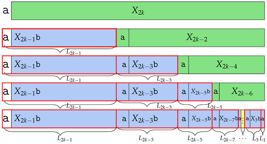
$L_{2k}^{♭}=\mathtt{a}{X}_{2k}$ is not a Lyndon word; therefore, its Lyndon is factorized and has more than one factor. According to Lemma 34, the Lyndon word of the Fibonacci word $F_{2k}=X_{2k}\mathtt{ab}$ is $\mathtt{a}{X}_{2k}\mathtt{b}$. The central word $X_{2k}$ is $X_{2k-1}ba{X}_{2k-2}$, so the Lyndon word of $F_{2k}$ is $\mathtt{a}{X}_{2k}\mathtt{b}=\mathtt{a}{X}_{2k-1}\mathtt{ba}{X}_{2k-2}\mathtt{b}$. $\mathtt{a}{X}_{2k-1}\mathtt{b}$ refers to $L_{2k-1}$, which is $\mathtt{a}{X}_{2k-1}\mathtt{b}$ and the suffix $\mathtt{a}{X}_{2k-2}\mathtt{b}$ is $L_{2k-2}$.

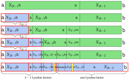
However, by deleting the last character $\mathtt{b}$, $L_{2k}^{♭}$ becomes $\mathtt{a}{X}_{2k-1}\mathtt{ba}{X}_{2k-2}$, meaning that $L_{2k-2}$ does not exist. Thus, we can say that $L_{2k-1}$ is one of the Lyndon factors, since it is not followed by $L_{2k-2}$. The remaining part of $L_{2k}^{♭}$ is $\mathtt{a}{X}_{2k-2}$. The same as $X_{2k}$, central word $X_{2k-2}$ can be divided as $X_{2k-3}\mathtt{ba}{X}_{2k-4}$; thus, $\mathtt{a}{X}_{2k-2}=\mathtt{a}{X}_{2k-3}\mathtt{ba}{X}_{2k-4}$. We can find Lyndon factor $L_{2k-3}=\mathtt{a}{X}_{2k-3}\mathtt{b}$ in the prefix. The remaining part is $\mathtt{a}{X}_{2k-4}$, which is not a Lyndon word, same as $\mathtt{a}{X}_{2k-2}$ above, so $\mathtt{a}{X}_{2k-4}$ is Lyndon factorized and makes $L_{2k-5}$ as a prefix, and the remaining $\mathtt{a}{X}_{2k-6}$ makes $L_{2k-7}$ as a prefix. And finally, $\mathtt{a}{X}_4$ is divided as $\mathtt{a}{X}_3\mathtt{ba}{X}_2$, where $X_2$ is $\epsilon$. Therefore, $L_{2k}^{♭}$’s Lyndon factor is $L_{2i-1}$ for $i\in [2..k]$ and the last remaining part $\mathtt{a}$ is the Lyndon word itself. Thus, $L_{2k}^{♭}$ has Lyndon factors $L_{2i-1}$ for every $i\in [2..k]$ and $\mathtt{a}$ as a Lyndon factor. The number of the Lyndon factor is k, which we depict in Figure 6. □

Figure 6. Factorization of $L_{2k}^{♭}$ into Lyndon factors studied in the proof of Theorem 5. $L_{2k}^{♭}$ has k Lyndon factors.

By Lemma 33 and Theorem 5, we conclude that the multiplicative sensitivity for deleting the last character of $L_{2k}$ is $\mathsf{\Omega }\left(k\right)$.

Theorem 6.

We let $L_{2k}^{♭}\#$ be the word obtained by substituting the last character $\mathtt{b}$ of $L_{2k}$ by #. Then, $\rho (L_{2k}^{♭}\#)\ge k+1.$

Proof. 

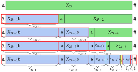
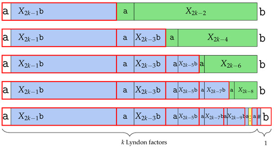
Since # is lexicographically smaller than $\mathtt{a}$, $L_{2k}^{♭}\#$ is not a Lyndon word; it makes Lyndon factors. Since # is smaller than both $\mathtt{a}$ and $\mathtt{b}$, # is a Lyndon word. In addition, $L_{2k}^{♭}$ is Lyndon factorized as Theorem 5, which produces Lyndon factors $L_{2i-1}$ for $i\in [2..k]$ and the last Lyndon factor $\mathtt{a}$. $L_{2k}^{♭}\#$ makes one more Lyndon factor, which is #, which therefore makes $k+1$ a number of Lyndon factors. We depict the Lyndon factorization in Figure 7. □

Figure 7. Factorization of $L_{2k}^{♭}\#$ into Lyndon factors studied in the proof of Theorem 6. $L_{2k}^{♭}\#$ has $k+1$ Lyndon factors.

By Lemma 33 and Theorem 6, we conclude that the multiplicative sensitivity for substituting the last character of $L_{2k}$ is $\mathsf{\Omega }\left(k\right)$. We observe a similar result when substituting the last character with a larger character instead of a smaller one (#).

Theorem 7.

$\rho \left(L_{2k}^{♭}\mathtt{c}\right)\ge k$.

Proof. 

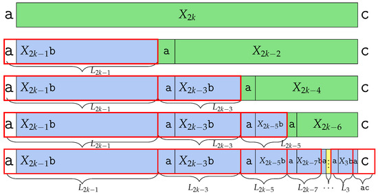
The lexicographic order between $\mathtt{a}$, $\mathtt{b}$, and $\mathtt{c}$ is $\mathtt{a}<\mathtt{b}<\mathtt{c}$. Recall that $L_{2k}^{♭}$ makes $L_{2i-1}$ for $i\in [2..k]$, and $\mathtt{a}$ as a Lyndon factor. In $L_{2k}^{♭}\mathtt{c}$, $\mathtt{c}$ is in position $f_{2k}$; therefore, it does not affect anything until the last Lyndon factor $\mathtt{a}$. $\mathtt{ac}$ is the Lyndon word itself because $\mathtt{a}<\mathtt{c}$. Therefore, $L_{2k}^{♭}\mathtt{c}$ makes a k number of Lyndon factors, shown in Figure 8. □

Figure 8. Factorization of $L_{2k}^{♭}\mathtt{c}$ into Lyndon factors studied in the proof of Theorem 7. $L_{2k}^{♭}\mathtt{c}$ has k Lyndon factors.

6.2. Insertions at Specific Locations

According to Corollary 1, $\rho$ is lower bounded by the number of distinct Lyndon factors. After editing $L_{2k}$ at any position, we can still find consecutive Lyndon conjugates of lower order which can merge to a higher order. For instance, $L_{2k-1}·L_{2k-2}$ merge into $L_{2k}$, which can decrease the number of the Lyndon factor. Also, $L_{2k-3}·L_{2k-2}$ merge into $L_{2k-1}$. Our idea is to avoid consecutive Fibonacci Lyndon conjugates so that they do not merge because doing so avoids a decrease in a number of distinct Lyndon factors. Now, we consider editing the specific location of Fibonacci Lyndon conjugates, also resulting in an increase in runs. The following theorems describe the bijective BWT of $L_{2k}$ after some specific edit operations are applied.

Theorem 8.

We let $L_{2k}$ be a Fibonacci Lyndon conjugate. By inserting $\mathtt{a}$ at position α in $L_{2k}$, ρ is at least k.

Proof. 

We let $\alpha$ be the number of additions of odd Fibonacci numbers $f_{2k-3}+f_{2k-5}+\cdots +f_3+f_1$. Recall that the Fibonacci word $F_i=X_{i}c$ with $c\in \{\mathtt{ab},\mathtt{ba}\}$ has the Lyndon conjugate $L_i=\mathtt{a}{X}_i\mathtt{b}$. Further, $L_{2k}=L_{2k-1}·L_{2k-2}=\mathtt{a}{X}_{2k-1}\mathtt{b}·\mathtt{a}{X}_{2k-2}\mathtt{b}$. Thus, we start with $\mathtt{a}{X}_{2k-1}\mathtt{b}·\mathtt{a}{X}_{2k-2}\mathtt{b}$. To obtain many distinct Lyndon factors, we aim to produce Lyndon factors that are not consecutive. Knowing $X_{2k-1}=X_{2k-3}\mathtt{ba}{X}_{2k-2}$, $\mathtt{a}{X}_{2k-2}$ merges with $\mathtt{a}{X}_{2k-3}\mathtt{b}$ into $L_{2k-1}$, so it is best to divide $X_{2k-2}$. $\mathtt{a}{X}_{2k-2}$ divides into $\mathtt{a}{X}_{2k-3}\mathtt{ba}{X}_{2k-4}$. In this case, it is best to add $\mathtt{a}{X}_{2k-3}\mathtt{b}$ as a new Lyndon factor since it is smallest among those Lyndon factors that are not consecutive with $X_{2k-1}$, the same as $\mathtt{a}{X}_{2k-2}$; $\mathtt{a}{X}_{2k-4}$ divides into $\mathtt{a}{X}_{2k-5}\mathtt{ba}{X}_{2k-6}$, and we add $\mathtt{a}{X}_{2k-5}\mathtt{b}$ as a Lyndon factor. $\mathtt{a}{X}_{2k-6}$ divides into $\mathtt{a}{X}_{2k-7}\mathtt{ba}{X}_{2k-8}$ as we add $\mathtt{a}{X}_{2k-7}\mathtt{b}$ as a Lyndon factor. The addition of Lyndon factors of $2i-1$ for $i\in [1..k-1]$ continues until $\mathtt{a}{X}_5=\mathtt{a}{X}_3\mathtt{ba}{X}_4$ appears since $\mathtt{a}{X}_3\mathtt{b}$ is the second smallest Lyndon factor in Fibonacci. Thus, we need $X_1=\mathtt{a}$ as the last Lyndon factor and it is obtained by inserting a # in $\mathtt{a}{X}_4$, dividing $\mathtt{a}{X}_4$ into $\mathtt{a}\#X_4$. Since # is lexicographically smaller than any words from right to #, the right words become the Lyndon factor. Thus, we can obtain k Lyndon factors by inserting # in $L_{2k}$: $k-1$ factors from $L_{2k-3}·L_{2k-5}\cdots L_1$ and one from # concatenated with the remaining words. And this is shown in Figure 9. □

Figure 9. Inserting # at position $\alpha$ in $L_{2k}$ considered in the proof in Theorem 8.

By Lemma 33 and Theorem 8, we conclude that the multiplicative sensitivity for inserting a character into $L_{2k}$ is $\mathsf{\Omega }\left(k\right)$. In the same way, we can also insert the special character # to observe a similar behavior:

Theorem 9.

We let $L_{2k}$ be a Fibonacci Lyndon conjugate. By inserting # at position $f_{2k}-2$ in $L_{2k}$, ρ is at least $k+1$.

Proof. 

Unlike Theorem 8, we can obtain some Lyndon factors on the right side of $\mathtt{a}{X}_{2k}\mathtt{b}$, adding $\mathtt{a}{X}_{2k-1}\mathtt{b}=L_{2k-1}$ as a Lyndon factor. We divide $\mathtt{a}{X}_{2k-2}\mathtt{b}$ into $\mathtt{a}{X}_{2k-3}\mathtt{ba}{X}_{2k-4}\mathtt{b}$ and obtain $\mathtt{a}{X}_{2k-3}\mathtt{b}=L_{2k-3}$. Further, we divide $\mathtt{a}{X}_{2k-4}\mathtt{b}$ into $\mathtt{a}{X}_{2k-5}\mathtt{ba}{X}_{2k-6}\mathtt{b}$, making $L_{2k-5}$. We divide $\mathtt{a}{X}_{2k-6}\mathtt{b}$ and can obtain Lyndon factors such as $L_{2k-7}\cdots L_5$. Lastly, $\mathtt{a}{X}_4\mathtt{b}$ divides into $\mathtt{a}{X}_3\mathtt{ba}{X}_2\mathtt{b}$, but since $X_2$ is $\epsilon$, the last Lyndon factor obtained here is $L_3$. To make more Lyndon factors, we can add # between $\mathtt{a}$ and $\mathtt{b}$, turning into $\mathtt{a}\#\mathtt{b}$, adding 2 Lyndon factors which are $\mathtt{a}=L_1$ and $\#\mathtt{b}$. Thus, we can obtain $k+1$ Lyndon factors here: k factors by $L_{2k-1},L_{2k-3}\cdots L_1$ and one from $\#\mathtt{b}$. We visualize the Lyndon factorization in Figure 10. □

Figure 10. Insertion of # at position $f_{2k}-2$ in $L_{2k}$ increases $\rho$ by at least the number of distinct Lyndon factors $k+1$ studied in Theorem 9.

7. Additive Sensitivity of $\mathit{\rho }$ by $\mathsf{\Omega }\left(\sqrt{\mathit{n}}\right)$

Here, we study the additive sensitivity of $\rho$ with an approach similar to Section 5. In what follows, we establish that the additive sensitivity of $\rho$ is at least $\Theta \left(\sqrt{n}\right)$. To that end, we again make use of the word $W_k$. Recall that $W_k=\left({\prod }_{i=2}^{k-1}{P}_i{E}_i\right)Q_k=\left({\prod }_{i=2}^{k-1}{\mathtt{ab}}^i{\mathtt{aaab}}^i{\mathtt{aba}}^{i-2}\right){\mathtt{ab}}^k\mathtt{a}$.

Lemma 36.

The Lyndon conjugate $C_k$ of $W_k$ is ${\mathtt{a}}^{k-2}{\mathtt{b}}^k\mathtt{a}·\left({\prod }_{i=2}^{k-2}{P}_i{E}_i\right)·P_{k-1}{\mathtt{ab}}^{k-1}\mathtt{ab}$.

Proof. 

The Lyndon conjugate of $W_k$ starts with the longest runs of $\mathtt{a}$, which can be obtained by concatenating suffix ${\mathtt{a}}^{k-3}$ of $E_{k-1}$ with prefix $\mathtt{a}$ of $Q_k$. Therefore, $C_k={\mathtt{a}}^{k-2}{\mathtt{b}}^k\mathtt{a}·\left({\prod }_{i=2}^{k-2}{P}_i{E}_i\right)·P_{k-1}{\mathtt{ab}}^{k-1}\mathtt{ab}={\mathtt{a}}^{k-2}{\mathtt{b}}^k\mathtt{a}·\left({\prod }_{i=2}^{k-2}{\mathtt{ab}}^i{\mathtt{aaab}}^i{\mathtt{aba}}^{i-2}\right)·{\mathtt{ab}}^{k-1}\mathtt{aa}{\mathtt{ab}}^{k-1}\mathtt{ab}$. □

Lemma 37.

$\rho \left(C_k\right)$ = $6k-12$.

Proof. 

According to Lemma 1, all conjugates have the same BWT, thus $r\left(W_k\right)=r\left(C_k\right)=6k-12$. Also, since $C_k$ is a Lyndon word, $r\left(C_k\right)=\rho \left(C_k\right)=6k-12$. □

Recall that the runs in the BBWT and BWT are the same if the input word is Lyndon, cf. Lemma 1. Thus, we can leverage BWT computation if the input word is Lyndon since we can obtain the number of runs in the same way as in Section 5 by using $\beta \left(W\right)$ for word W. In this section, we focus on three variations of the word $C_k$: deleting its last character and substituting its last character $\mathtt{b}$ with $\mathtt{c}$ or #.

7.1. Deletions and Edits of $C_k$ with a Character Smaller than $\mathtt{a}$

Recall that $C_k={\mathtt{a}}^{k-2}{\mathtt{b}}^k\mathtt{a}·\left({\prod }_{i=2}^{k-2}{\mathtt{ab}}^i{\mathtt{aaab}}^i{\mathtt{aba}}^{i-2}\right)·{\mathtt{ab}}^{k-1}\mathtt{aa}{\mathtt{ab}}^{k-1}\mathtt{ab}$. Thus, $C_k^{♭}$, which is obtained by deleting the last character $\mathtt{b}$, is $C_k^{♭}={\mathtt{a}}^{k-2}{\mathtt{b}}^k\mathtt{a}·\left({\prod }_{i=2}^{k-2}{\mathtt{ab}}^i{\mathtt{aaab}}^i{\mathtt{aba}}^{i-2}\right)·{\mathtt{ab}}^{k-1}\mathtt{aa}{\mathtt{ab}}^{k-1}\mathtt{a}$. Recall that the Lyndon conjugate of $C_k^{♭}$ is the strictly smallest conjugate of all conjugates of $C_k^{♭}$. Since we obtain the longest runs of $\mathtt{a}$s from a conjugate of $C_k^{♭}$ by concatenating the last $\mathtt{a}$ with ${\mathtt{a}}^{k-2}{\mathtt{b}}^k\mathtt{a}$, $C_k^{♭}$ cannot be a Lyndon word. In fact, it has two Lyndon factors, which are ${\mathtt{a}}^{k-2}{\mathtt{b}}^k\mathtt{a}·\left({\prod }_{i=2}^{k-2}{\mathtt{ab}}^i{\mathtt{aaab}}^i{\mathtt{aba}}^{i-2}\right)·{\mathtt{ab}}^{k-1}\mathtt{aa}{\mathtt{ab}}^{k-1}$, and we refer to both Lyndon factors as $D_k$ (first factor) and $\mathtt{a}$ from now on. Figure 11 shows the Lyndon factorization. Since $r\left(\mathtt{a}\right)$ is 1, the only thing left to check is $r\left(D_k\right)$. In $D_k$, we made a slight modification to the subword $E_{k-1}$. In fact, $E_{k-1}={\mathtt{ab}}^{k-1}{\mathtt{aba}}^{k-3}$ was changed to ${\mathtt{ab}}^{k-1}{\mathtt{a}}^{k-3}$, which we call $H_{k-1}$ in this section. Since $D_k$ is a Lyndon word, we determine $\rho \left(D_k\right)$ using $\mathcal{M}\left(D_k\right)$ with the BWT as we did before.

Figure 11. Introducing $D_k$ from $C_k^{♭}$ studied in Section 7.1. $D_k$ is the first Lyndon factor of $C_k^{♭}$.

Lemma 38.

$\beta ({\mathtt{a}}^{k-2}\mathtt{b},D_k)=\mathtt{b}$.

Proof. 

The only conjugate in $\mathcal{M}\left(D_k\right)$ starting with prefix ${\mathtt{a}}^{k-2}\mathtt{b}$ is ${\mathtt{a}}^{k-2}\mathtt{b}{P}_2\cdots \mathtt{b}$. The first conjugate in lexicographic order must start with the longest run of $\mathtt{a}$. By the definition of $D_k$, the longest run of $\mathtt{a}$ has length $k-2$, and it is obtained by concatenating suffix ${\mathtt{a}}^{k-3}$ with prefix $\mathtt{a}$ of $Q_k$ that is preceded by $\mathtt{b}$ (otherwise, we could extend the sequence of $\mathtt{a}$ characters). □

Lemma 39.

$\beta ({\mathtt{a}}^i\mathtt{b},D_k)={\mathtt{ba}}^{k-i-2}$, for all $i\in [4..k-3]$.

Proof. 

With integer $i\in [3..k-3]$, the conjugates in $\mathcal{M}\left(D_k\right)$ starting with ${\mathtt{a}}^i\mathtt{b}$ are

$$\begin{array}{c}\hfill {\mathtt{a}}^{i-1}{P}_{i+2}\cdots \mathtt{b}<{\mathtt{a}}^{i-1}{P}_{i+3}\cdots \mathtt{a}<\cdots <{\mathtt{a}}^{i-1}{P}_{k-1}\cdots \mathtt{a}<{\mathtt{a}}^i{\mathtt{b}}^k\mathtt{a}{P}_2\cdots \mathtt{a}.\end{array}$$

For all $i\in [4..k-3]$, the factor ${\mathtt{a}}^i\mathtt{b}$ can only be obtained from the concatenation of suffix ${\mathtt{a}}^{i-1}$ from $E_{j-1}$,

• with the prefix $\mathtt{ab}$ of $P_j$ for a $j\in [i+2..k-1]$ or
• with the prefix $\mathtt{ab}$ of $Q_k$, if $j=k$.

We can sort these conjugates according to the lexicographic order of ${\bigcup }_{j=i+2}^{k-1}{P}_j\cup Q_k$. All these conjugates end with an $\mathtt{a}$, with the exception of the conjugate starting with ${\mathtt{a}}^i{P}_{i+2}$, since $D_k$ has a unique occurrence of ${\mathtt{ba}}^i\mathtt{b}$. □

Lemma 40.

$\beta (\mathtt{aaab},D_k)=\mathtt{bbbbb}{\left(\mathtt{ab}\right)}^{k-7}\mathtt{baa}$.

Proof. 

The conjugates in $\mathcal{M}\left(D_k\right)$ starting with $\mathtt{aaab}$ are

$$\begin{array}{cc}\hfill \mathtt{aa}{E}_2\cdots \mathtt{b}& <\mathtt{aa}{E}_3\cdots \mathtt{b}<\mathtt{aa}{E}_4\cdots \mathtt{b}<\mathtt{aa}{P}_5\cdots \mathtt{b}<\mathtt{aa}{E}_5\cdots \mathtt{b}\hfill \\ & <\mathtt{aa}{P}_6\cdots \mathtt{a}<\mathtt{aa}{E}_6\cdots \mathtt{b}<\cdots <\mathtt{aa}{P}_{k-2}\cdots \mathtt{a}<\mathtt{aa}{E}_{k-2}\cdots \mathtt{b}\hfill \\ & <\mathtt{aa}{H}_{k-1}\cdots \mathtt{b}<\mathtt{aa}{P}_{k-1}\cdots \mathtt{a}<\mathtt{aa}{Q}_k\cdots \mathtt{a}.\hfill \end{array}$$

The above conjugates are obtained in the following cases.

Case 1:

  by concatenating the suffix $\mathtt{aa}$ of $E_{i-1}$ with the prefix $\mathtt{ab}$ of $P_i$, if only $i\in [5..k-1]$,

Case 2:

  by concatenating the suffix $\mathtt{aa}$ of $P_i$, with the prefix $\mathtt{ab}$ of $E_i$, for all $i\in [2..k-2]$ or with $H_{k-1}$ if $i=k-1$,

Case 3:

  by concatenating the suffix $\mathtt{aa}$ of $H_{k-1}$ with the prefix $\mathtt{ab}$ of $Q_k$.

All these conjugates starting with $\mathtt{aaab}$ are sorted according to the lexicographic order of the words in ${\bigcup }_{i=2}^4\left\{\mathtt{aa}{E}_i\right\}\cup {\bigcup }_{j=5}^{k-2}\{\mathtt{aa}{P}_j·\mathtt{aa}{E}_j\}\cup \left\{\mathtt{aa}{H}_{k-1}\right\}\cup \left\{\mathtt{aa}{P}_{k-1}\right\}\cup \left\{\mathtt{aa}{Q}_k\right\}.$ The conjugates starting either with $\mathtt{aa}{P}_i$, for all $i\in [6..k-1]$ in Case 1 or Case 3, end with an $\mathtt{a}$. On the other hand, conjugates of Case 2 or $\mathtt{aa}{P}_5$ in Case 1 end with a $\mathtt{b}$. □

Lemma 41.

$\beta (\mathtt{aab},D_k)={\mathtt{baaba}}^{2k-8}.$

Proof. 

The conjugates in $\mathcal{M}\left(D_k\right)$ starting with $\mathtt{aab}$ are

$$\begin{array}{cc}\hfill \mathtt{a}{P}_2\cdots \mathtt{b}& <\mathtt{a}{E}_2\cdots \mathtt{a}<\mathtt{a}{E}_3\cdots \mathtt{a}<\mathtt{a}{P}_4\cdots \mathtt{b}<\mathtt{a}{E}_4\cdots \mathtt{a}\hfill \\ & <\mathtt{a}{P}_5\cdots \mathtt{a}<\mathtt{a}{E}_5\cdots \mathtt{a}<\cdots <\mathtt{a}{H}_{k-1}\cdots \mathtt{a}<\mathtt{a}{P}_{k-1}\cdots \mathtt{a}<\mathtt{a}{Q}_k\cdots \mathtt{a}.\hfill \end{array}$$

Each of the cases from Case 1 to Case 3 in Lemma 40 induces a conjugate starting with $\mathtt{aab}$, obtained by shifting on the left character $\mathtt{a}$. It follows that all of these conjugates end with $\mathtt{a}$. The other two conjugates that start with an $\mathtt{aab}$ are obtained by

• concatenating the suffix $\mathtt{a}$ of $Q_k$ with the prefix $\mathtt{ab}$ of $P_2$ or
• concatenating suffix $\mathtt{a}$ of $E_3$ to the prefix $\mathtt{ab}$ of $P_4$.

In both cases, the obtained conjugates end with $\mathtt{b}$. We conclude this proof by sorting lexicographically the conjugates in $\mathtt{a}{P}_2\cup {\bigcup }_{i=2}^3\left\{\mathtt{a}{E}_i\right\}\cup {\bigcup }_{i^{\prime }=4}^{k-2}\{\mathtt{a}{P}_{i^{\prime }}·\mathtt{a}{E}_{i^{\prime }}\}\cup \left\{\mathtt{a}{H}_{k-1}\right\}\cup \left\{\mathtt{a}{P}_{k-1}\right\}\cup \left\{\mathtt{a}{Q}_k\right\}.$ □

Lemma 42.

$\beta (\mathtt{ab},D_k)={\mathtt{b}}^{k-3}{\mathtt{aaba}}^{2k-6}.$

Proof. 

The conjugates in $\mathcal{M}\left(D_k\right)$ starting with $\mathtt{ab}$ are

$$\begin{array}{cc}\hfill {\mathtt{aba}}^{k-4}{P}_{k-1}\cdots \mathtt{b}& <\cdots <\mathtt{ab}{P}_3\cdots \mathtt{b}\hfill \\ & <P_2\cdots \mathtt{a}<E_2\cdots \mathtt{a}<P_3\cdots \mathtt{b}\hfill \\ & <E_3\cdots \mathtt{a}<P_4\cdots \mathtt{a}<E_4\cdots \mathtt{a}<\cdots <P_{k-2}\cdots \mathtt{a}<E_{k-2}\cdots \mathtt{a}\hfill \\ & <H_{k-1}\cdots \mathtt{a}<P_{k-1}\cdots \mathtt{a}<Q_k\cdots \mathtt{a}.\hfill \end{array}$$

The above conjugates are obtained in the following cases.

Case 1:

  $P_i$ for all $i\in [2..k-1]$,

Case 2:

  prefix $\mathtt{ab}$ of $E_i$, for all $i\in [2..k-1]$,

Case 3:

  ${\mathtt{aba}}^{i-2}$ from $E_i$, for all $i\in [2..k-2]$ or $\mathtt{ab}$ from $H_{k-1}$,

Case 4:

  $\mathtt{ab}$ from $Q_k$.

For two distinct integers $i,i^{\prime }$ with $i>i^{\prime }\ge 0$, we have ${\mathtt{aba}}^i>{\mathtt{aba}}^{i^{\prime }}$. Thus, the first conjugate in lexicographic order starting with $\mathtt{ab}$ is the one followed by the longest run of $\mathtt{a}$s. The smallest of these conjugates can be found by concatenating the suffix ${\mathtt{aba}}^{k-4}$ with the prefix $\mathtt{ab}$ of $P_{k-1}$ from Case 3. Then, the remaining conjugates in Case 3 which are ${\mathtt{aba}}^{i-2}$ of $E_i$ for all $i\in [2..k-3]$ follow in decreasing order. By construction of $E_i$, for all $i\in [2..k-2]$, these conjugates must end with a $\mathtt{b}$. Note that the remaining cases are obtained by shifting the character $\mathtt{a}$ from the conjugates starting with $\mathtt{aab}$ from Lemma 41 with the exception of the character starting with $P_3$. It follows that the latter ends with a $\mathtt{b}$, while all the other conjugates end with $\mathtt{a}$. □

Lemma 43.

$\beta (\mathtt{ba},D_k)={\mathtt{ba}}^{k-6}{\mathtt{bbbab}}^{k-4}{\mathtt{ab}}^{k-3}\mathtt{a}.$

Proof. 

The conjugates in $\mathcal{M}\left(D_k\right)$ starting with $\mathtt{ab}$ are

$$\begin{array}{cc}\hfill {\mathtt{ba}}^{k-2}{\mathtt{b}}^k\mathtt{a}{P}_2\cdots \mathtt{b}& <{\mathtt{ba}}^{k-4}{P}_{k-1}\cdots \mathtt{a}<{\mathtt{ba}}^{k-5}{P}_{k-2}\cdots \mathtt{a}<\cdots <\mathtt{baaa}{P}_6\cdots \mathtt{a}\hfill \\ & <\mathtt{baa}{E}_2\cdots \mathtt{b}<\mathtt{baa}{E}_3\cdots \mathtt{b}<\mathtt{baa}{E}_4\cdots \mathtt{b}<\mathtt{baa}{P}_5\cdots \mathtt{a}\hfill \\ & <\mathtt{baa}{E}_5\cdots \mathtt{b}<\cdots <\mathtt{baa}{E}_{k-2}\cdots \mathtt{b}<\mathtt{baa}{H}_{k-1}\cdots \mathtt{b}<\mathtt{ba}{P}_2\cdots \mathtt{b}\hfill \\ & <\mathtt{ba}{P}_4\cdots \mathtt{a}\hfill \\ & <{\mathtt{baba}}^{k-4}{P}_{k-1}\cdots \mathtt{b}<\cdots <\mathtt{bab}{P}_3\cdots \mathtt{b}\hfill \\ & <\mathtt{b}{P}_3\cdots \mathtt{a}.\hfill \end{array}$$

The conjugates above are obtained by following cases.

Case 1:

suffix $\mathtt{baa}$ of $P_i$ concatenating with $E_i$ for all $i\in [2..k-2]$ or $H_{k-1}$ if $i=k-1$,

Case 2:

runs in $E_i$ for all $i\in [2..k-2]$,

Case 3:

suffix $\mathtt{ba}$ from $Q_k$ concatenating with $P_2$,

Case 4:

${\mathtt{ba}}^{k-3}$ of $H_{k-1}$ concatenating with $Q_k$.

We have as many circular occurrences of $\mathtt{ba}$ as the number of maximal runs of $\mathtt{b}$s in $D_k$. For Case 1, we have one conjugate starting with $\mathtt{baa}{E}_i$ for all $i\in [2..k-2]$ or $\mathtt{baa}$$H_{k-1}$. Since each run of $\mathtt{b}$s within each word from ${\bigcup }_2^{k-1}{P}_i$ is of length of at least 2, all conjugates of Case 1 end with $\mathtt{b}$.

For Case 2, for all $i\in [2..k-2]$, we can distinguish two subcases based on where $\mathtt{ba}$ starts:

Case 2 (a):

 the first run of $\mathtt{ba}$ in $E_i$, which has a type of ${\mathtt{baba}}^{i-2}$ for all $i\in [2..k-2]$,

Case 2 (b):

 the second run of $\mathtt{ba}$ in $E_i$, which has a type of ${\mathtt{ba}}^{i-2}$ for all $i\in [2..k-2]$.

• For Case 2 (a), we can see that these conjugates start with ${\mathtt{baba}}^{i-2}{P}_{i+1},$ if $i\in [2..k-2]$. Similarly to Case 1, each conjugate for Case 2 (a) ends with a $\mathtt{b}$. Each conjugate in Case 2 (b) is obtained by shifting two characters on the right each conjugate in Case 2 (a). Therefore, all of these conjugates end with an $\mathtt{a}$ and have prefixes of the type ${\mathtt{ba}}^{i-2}{P}_{i+1}$, if $i\in [2..k-2]$.
• For Case 3, the conjugate starting with $\mathtt{ba}$ in $Q_k$ has $\mathtt{ba}{P}_2$ as a prefix, and it is preceded by a $\mathtt{b}$.
• Lastly, for Case 4, the conjugates start with ${\mathtt{ba}}^{k-3}$ concatenating with $Q_k$ which ends with a $\mathtt{b}$.
• Observe that only for Case 4 and Case 2 (b) we have conjugates starting with $\mathtt{baaaa}$. Hence, the first conjugate in lexicographic order is the one from Case 4 starting with ${\mathtt{ba}}^{k-3}{Q}_k$, followed by those from Case 2 (b) which are ${\mathtt{ba}}^{k-4}{P}_{k-1}<{\mathtt{ba}}^{k-5}{P}_{k-2}<\cdots <\mathtt{baaa}{P}_6$.

Among the remaining conjugates, those having prefix $\mathtt{baaa}$ either start with $\mathtt{baa}{P}_5$ from Case 2 (b) and from Case 1 starting with $\mathtt{baa}{E}_i$ for all $i\in [2..k-2]$ or $\mathtt{baa}$$H_{k-1}$ if $i=k-1$. We can sort them according to the order of the words in

$$\bigcup _{i=2}^4\left\{\mathtt{baa}{E}_i\right\}\cup \left\{\mathtt{baa}{P}_5\right\}\cup \bigcup _{i=5}^{k-2}\left\{\mathtt{baa}{E}_i\right\}\cup \left\{\mathtt{baa}{H}_{k-1}\right\}.$$

Then, the remaining conjugates with prefix $\mathtt{baa}$ are those starting with $\mathtt{ba}{P}_2$ from Case 3 and $\mathtt{ba}{P}_4$ from Case 2 (b). Finally, let us focus on the conjugates from Case 2 (a). These conjugates are sorted according to the length of the run of $\mathtt{a}$s following the common prefix $\mathtt{bab}$. The last conjugate left is the one starting with $\mathtt{b}{P}_3$ from Case 2 (b). Since this conjugate is greater than each conjugate considered in Case 2 (a), this is the greatest conjugate of $D_k$ starting with $\mathtt{ba}$ and the thesis follows. □

Lemma 44.

$\beta ({\mathtt{b}}^j\mathtt{a},D_k)={\mathtt{bab}}^{2k-2j-2}\mathtt{a}$ for all $j\in [2..k-2]$.

Proof. 

With integer $i\in [2..k-2]$, the conjugates in $\mathcal{M}\left(D_k\right)$ starting with the prefix ${\mathtt{b}}^i\mathtt{a}$ are

$$\begin{array}{cc}\hfill {\mathtt{b}}^i{\mathtt{a}}^{k-3}{Q}_k\cdots \mathtt{b}& <{\mathtt{b}}^i\mathtt{aa}{E}_i\cdots \mathtt{a}<{\mathtt{b}}^i\mathtt{aa}{E}_{i+1}\cdots \mathtt{b}<\cdots <{\mathtt{b}}^i\mathtt{aa}{E}_{k-2}\cdots \mathtt{b}<{\mathtt{b}}^i\mathtt{aa}{H}_{k-1}\cdots \mathtt{b}\hfill \\ & <{\mathtt{b}}^i\mathtt{a}{P}_2\cdots \mathtt{b}<{\mathtt{b}}^i{\mathtt{aba}}^{k-4}{P}_{k-1}\cdots \mathtt{b}<\cdots <{\mathtt{b}}^i{\mathtt{aba}}^{i-1}{P}_{i+2}\cdots \mathtt{b}\hfill \\ & <{\mathtt{b}}^i{\mathtt{aba}}^{i-2}{P}_{i+1}\cdots \mathtt{a}.\hfill \end{array}$$

Case 1:

  concatenating ${\mathtt{b}}^i$$\mathtt{aa}$ of $P_j$ with $E_j$ for all $j\in [i..k-1]$ or with $H_{k-1}$ if only $j=k-1$,

Case 2:

  concatenating ${\mathtt{b}}^i{\mathtt{aba}}^{j-2}$ of $E_j$ with $P_{j+1}$ if only $j\in [i..k-2]$,

Case 3:

  concatenating ${\mathtt{b}}^i{\mathtt{a}}^{k-3}$ of $H_{k-1}$ with $Q_k$,

Case 4:

  concatenating ${\mathtt{b}}^i\mathtt{a}$ with $P_2$.

We consider these four cases separately. For all $j\in [i..k-2]$, the conjugate starting within $P_j$ has a prefix of ${\mathtt{b}}^i\mathtt{aa}{E}_j$ or ${\mathtt{b}}^i\mathtt{aa}{H}_{k-1}$ (Case 1). For all $j\in [i..k-2]$, the conjugates starting within $E_j$ have a prefix of ${\mathtt{b}}^i{\mathtt{aba}}^{j-2}{P}_{j+1}$ (Case 2). In addition, conjugate starting within a word in Case 3 has a prefix of ${\mathtt{b}}^i{\mathtt{a}}^{k-3}{Q}_k$. Finally, the conjugates starting with $Q_k$ starts with ${\mathtt{b}}^i\mathtt{a}{P}_2$ (Case 4). By construction, we can see that first we have all the conjugates first from Case 3 and then from Case 1 sorted according to the lexicographic order into ${\bigcup }_{j=i}^{k-2}{\mathtt{b}}^i\mathtt{aa}{E}_j\cup {\mathtt{b}}^i\mathtt{aa}{H}_{k-1}$; then, we have the conjugate from Case 4, then Case 2 sorted according to the decreasing length of the run of $\mathtt{a}$s following the common prefix ${\mathtt{b}}^i\mathtt{ab}$. Moreover, we note that only when the run of $\mathtt{b}$s is exactly of length $\mathtt{i}$, the conjugate ends with $\mathtt{a}$. Thus, only the conjugates ending with an $\mathtt{a}$ are those starting within ${\mathtt{b}}^i\mathtt{aa}{E}_i$ and ${\mathtt{b}}^i{\mathtt{aba}}^{i-2}{P}_{i+1}$. □

Lemma 45.

β(${\mathtt{b}}^{k-1}\mathtt{a},D_k$)= $\mathtt{aab}$.

Proof. 

There are three conjugates in $\mathcal{M}\left(D_k\right)$ starting with prefix ${\mathtt{b}}^{k-1}\mathtt{a}$. These conjugates are

$$\begin{array}{c}\hfill {\mathtt{b}}^{k-1}{\mathtt{a}}^{k-3}{Q}_k\cdots \mathtt{a}<{\mathtt{b}}^{k-1}{\mathtt{aaab}}^{k-1}\cdots \mathtt{a}<{\mathtt{b}}^{k-1}\mathtt{a}{P}_2\cdots \mathtt{b}.\end{array}$$

Observe that the only conjugates with prefix ${\mathtt{b}}^{k-1}\mathtt{a}$ have the prefixes, respectively, of ${\mathtt{b}}^{k-1}{\mathtt{a}}^{k-3}{Q}_k$, ${\mathtt{b}}^{k-1}\mathtt{aa}{H}_{k-1}$, and ${\mathtt{b}}^{k-1}\mathtt{a}{P}_2$. One can see that these conjugates taken in this order are already sorted, and only the conjugate starting within $Q_k$ ends with $\mathtt{b}$, while the other two have $\mathtt{a}$. □

Lemma 46.

$\beta ({\mathtt{b}}^k\mathtt{a},D_k)=\mathtt{a}$.

Proof. 

The last conjugate in $\mathcal{M}\left(D_k\right)$ with prefix ${\mathtt{b}}^k\mathtt{a}$ is ${\mathtt{b}}^k\mathtt{a}{P}_2\cdots \mathtt{a}$. Finally, the only occurrence of ${\mathtt{b}}^k$ is within $Q_k$. Hence, the last conjugate in lexicographic order starts with ${\mathtt{b}}^k\mathtt{a}{P}_2$, and since the run of $\mathtt{b}$’ is maximal, it ends with an $\mathtt{a}$, and the thesis follows. □

We summarize the above lemmas as follows.

Lemma 47.

For integer$k\ge 10$, $\rho \left(D_k\right)=8k-18$, cf. Table 14. The BWT of the word $D_k$ is given by $\mathrm{BBWT}\left(D_k\right)={\prod }_{i=2}^{k-1}\beta \left({\mathtt{a}}^{k-i}\mathtt{b}\right)·{\prod }_{i=1}^k\beta \left({\mathtt{b}}^i\mathtt{a}\right)$.

Table 14. Classification of the number of runs obtain in Lemma 47. The total number of runs is $8k-18$.

BBWT of $\overline{{\mathit{W}}_{\mathit{k}}^{♭}}\mathtt{c}$	Runs
$\beta \left({\mathtt{a}}^{k-2}\mathtt{b}\right)=\mathtt{b}$	1
$\beta \left({\mathtt{a}}^i\mathtt{b}\right)={\mathtt{ba}}^{k-i-2}$, for all $i\in [4..k-3]$	$2k-12$ but, when merged, $2k-13$
$\beta \left(\mathtt{aaab}\right)=\mathtt{bbbbb}{\left(\mathtt{ab}\right)}^{k-7}\mathtt{baa}$	$2k-12$
$\beta$($\mathtt{aab}$) = ${\mathtt{baaba}}^{2k-8}$	4
$\beta$($\mathtt{ab}$) = ${\mathtt{b}}^{k-3}{\mathtt{aaba}}^{2k-6}$	4
$\beta \left(\mathtt{ba}\right)={\mathtt{ba}}^{k-6}{\mathtt{bbbab}}^{k-4}{\mathtt{ab}}^{k-3}\mathtt{a}$	8
$\beta \left({\mathtt{b}}^j\mathtt{a}\right)={\mathtt{bab}}^{2k-2j-2}\mathtt{a}$ for all $j\in [2..k-2]$	$4k-12$
$\beta$(${\mathtt{b}}^{k-1}\mathtt{a}$) = $\mathtt{aab}$	2 but, when merged, 1
$\beta$(${\mathtt{b}}^k\mathtt{a}$) = $\mathtt{a}$	1

Proof. 

Every conjugate of $\beta \left({\mathtt{a}}^i\mathtt{b}\right)$ is smaller than each conjugate of $\beta \left({\mathtt{a}}^{i^{\prime }}\mathtt{b}\right)$ for every $1\le i^{\prime }<i\le k-2$. Symmetrically, every conjugate of $\beta \left({\mathtt{b}}^j\mathtt{a}\right)$ is greater than any conjugate of $\beta \left({\mathtt{b}}^{j^{\prime }}\mathtt{a}\right)$, for every $1\le j^{\prime }<j\le k$. Since we considered all the disjoint ranges of conjugates of $D_k$ based on their common prefix, the word ${\prod }_{i=2}^{k-1}\beta \left({\mathtt{a}}^{k-i}\mathtt{b}\right)·{\prod }_{i=1}^k\beta \left({\mathtt{b}}^i\mathtt{a}\right)$ is the BWT of $D_k$.

With the structure of $\mathrm{BBWT}\left(D_k\right)$, we can easily derive its number of runs. The word ${\prod }_{i=2}^{k-4}\beta \left({\mathtt{a}}^{k-i}\mathtt{b}\right)$ has exactly $2(k-6)$ runs. We start with 2 runs from $\beta \left({\mathtt{a}}^{k-2}\mathtt{b}\right)\beta \left({\mathtt{a}}^{k-3}\mathtt{b}\right)=\mathtt{bba},$ and then, concatenating each $\beta \left({\mathtt{a}}^i\mathtt{b}\right)$ up to $\beta \left({\mathtt{a}}^4\mathtt{b}\right)$ adds 2 new runs each. By counting, we observe that $\beta \left(\mathtt{aaab}\right),\beta \left(\mathtt{aab}\right),\beta \left(\mathtt{ab}\right)$ have $2(k-6)$, 4, 4. The boundaries between these words do not yet merge. The word $\beta \left(\mathtt{ba}\right)$ has exactly 8 runs. The remaining part of the BWT, that is, ${\prod }_{i=2}^k\beta \left({\mathtt{b}}^i\mathtt{a}\right)$, has $4(k-3)+2$ runs. Concatenating each $\beta \left({\mathtt{b}}^2\mathtt{a}\right)$ to $\beta \left({\mathtt{b}}^{k-2}\mathtt{a}\right)$ adds 4 new runs each. The word $\beta \left({\mathtt{b}}^k\mathtt{a}\right)$ adds only one run by $\mathtt{b}$, as it contains an $\mathtt{a}$ that merges with the previous one. Finally, $\beta \left({\mathtt{b}}^k\mathtt{a}\right)$ adds one run. Altogether, we have $2(k-6)+2(k-6)+4+4+8+4(k-3)+2=8k-18$, and the claim holds. □

Using Lemma 47 above, we can finally obtain the runs of $C_k^{♭}=D_k\mathtt{a}$.

Theorem 10.

$\rho \left(C_k^{♭}\right)=8k-17$.

Proof. 

$C_k^{♭}={\mathtt{a}}^{k-2}{\mathtt{b}}^k\mathtt{a}·\left({\prod }_{i=2}^{k-2}{\mathtt{ab}}^i{\mathtt{aaab}}^i{\mathtt{aba}}^{i-2}\right)·{\mathtt{ab}}^{k-1}\mathtt{aa}{\mathtt{ab}}^{k-1}\mathtt{a}$. The Lyndon conjugate of $C_k^{♭}$ is the smallest conjugate starting with the longest runs of $\mathtt{a}$, thus it is the one starting with ${\mathtt{a}}^{k-1}$. Therefore, it is obvious that $C_k^{♭}$ is not a Lyndon word, then it is Lyndon factorized by an $\mathtt{a}$ and the residual which is $D_k$. Figure 12 depicts the Lyndon factorization of $C_k^{♭}$. Since the lexicographic order between $\mathtt{a}$ and $D_k$ is $\mathtt{a}$$<D_k$, the runs of $C_k^{♭}$ add one run because the first conjugate of $D_k$ from Lemma 38 ends with a $\mathtt{b}$. Therefore, $\rho \left(C_k^{♭}\right)=\rho \left(\mathtt{a}\right)+\rho \left(D_k\right)=8k-17$. □

Figure 12. Lyndon factorization of $C_k^{♭}$. We obtain $\rho \left(C_k^{♭}\right)$ by knowing the number of runs of both its Lyndon factors and where these conjugates are sorted in the BBWT. The analysis is in the proof of Theorem 10.

With Lemma 37 and Theorem 10, we determine that the additive sensitivity of $\rho$ for $C_k$ is $\Theta (logn)$ when deleting the last character.

Theorem 11.

$\rho (C_k^{♭}$#)= $8k-16$.

Proof. 

$C_k^{♭}$# = ${\mathtt{a}}^{k-2}{\mathtt{b}}^k\mathtt{a}·\left({\prod }_{i=2}^{k-2}{\mathtt{ab}}^i{\mathtt{aaab}}^i{\mathtt{aba}}^{i-2}\right)·{\mathtt{ab}}^{k-1}\mathtt{aa}{\mathtt{ab}}^{k-1}\mathtt{a}$#. $C_k^{♭}\#$ is Lyndon factorized into three parts, which are $D_k$, $\mathtt{a}$ and #, because the lexicographic order of $\mathtt{a}$ is lower than $D_k$, and moreover # is smaller than both $D_k$ and $\mathtt{a}$. Therefore, the $\rho (C_k^{♭}\#)=\rho (\#)+\rho \left(\mathtt{a}\right)+\rho \left(D_k\right)=8k-16$. We show a sketch in Figure 13. □

Figure 13. Lyndon factorization of $C_k^{♭}\#$. Compared to Figure 12, we have one additional Lyndon factor. The analysis is in proof of Theorem 11.

With Lemma 37 and Theorem 11, we obtain that the additive sensitivity of $\rho$ for $C_k$ is $\Theta (logn)$ when substituting the last character.

7.2. Editing $C_k$ with a Character Larger than $\mathtt{b}$

Now, we consider the editing operation $C_k$ with a character $\mathtt{c}$ that is lexicographically larger than any character in $C_k$. In this part, we consider two edit operations that add $\mathtt{c}$ in the last part of $C_k$, and substitute the last character of $C_k$ into $\mathtt{c}$.

7.2.1. Appending $\mathtt{c}$ to $C_k$

Now, we prove that adding $\mathtt{c}$ to $C_k$, i.e., $C_k$ becomes $C_k\mathtt{c}$, also adds $\Theta \left(\sqrt{n}\right)$ in runs in BBWT. $C_k\mathtt{c}={\mathtt{a}}^{k-2}{\mathtt{b}}^k\mathtt{a}·\left({\prod }_{i=2}^{k-2}{\mathtt{ab}}^i{\mathtt{aaab}}^i{\mathtt{aba}}^{i-2}\right)·{\mathtt{ab}}^{k-1}\mathtt{aa}{\mathtt{ab}}^{k-1}\mathtt{abc}$. We illustrate $C_k$ in Figure 14. Similar to Section 7.1, we slightly modify $E_{k-1}$ to ${\mathtt{ab}}^{k-1}{\mathtt{abca}}^{k-3}$. In this section, we call this modified subword $S_{k-1}$. The lexicographic order of $\mathtt{c}$ is larger than any words in $C_k$. Thus, $C_k\mathtt{c}$ is a Lyndon word itself. Recall that the runs of a Lyndon word are the same in both the BWT or the BBWT, so we obtain $\rho \left(C_k\mathtt{c}\right)$ by using BWT with $\mathcal{M}\left(C_k\mathtt{c}\right)$ the same way we did in previous lemmas.

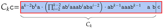
Figure 14. Introducing the Lyndon word $C_k\mathtt{c}$ studied in Section 7.2.

Lemma 48.

$\beta ({\mathtt{a}}^{k-2}\mathtt{b},C_k\mathtt{c})=\mathtt{c}$.

Proof. 

The first conjugate in $\mathcal{M}\left(C_k\mathtt{c}\right)$ is ${\mathtt{a}}^{k-2}\mathtt{ba}{P}_2\cdots \mathtt{c}$. The first conjugate must start with the longest run of $\mathtt{a}$s. In $C_k\mathtt{c}$, the longest run of $\mathtt{a}$ has a length of $k-2$ which is a prefix of itself, and it is obtained by concatenating the suffix ${\mathtt{a}}^{k-3}$ of $S_{k-1}$ with $Q_k$, and it is preceded by a $\mathtt{c}$. □

Lemma 49.

$\beta ({\mathtt{a}}^i\mathtt{b},C_k\mathtt{c})={\mathtt{ba}}^{k-i-2}$ for all $i\in [4..k-3]$.

Proof. 

In $\mathcal{M}\left(C_k\mathtt{c}\right)$, the conjugates starting with ${\mathtt{a}}^i\mathtt{b}$ for $i\in [4..k-3]$ are

$$\begin{array}{c}\hfill {\mathtt{a}}^{i-1}{P}_{i+2}\cdots \mathtt{b}<{\mathtt{a}}^{i-1}{P}_{i+3}\cdots \mathtt{a}<\cdots <{\mathtt{a}}^{i-1}{P}_{k-1}\cdots \mathtt{a}<{\mathtt{a}}^{i-1}{Q}_k\cdots \mathtt{a}.\end{array}$$

For all $i\in [4..k-3]$, the factor ${\mathtt{a}}^i\mathtt{b}$ can only be obtained, for all $j\in [i+2..k]$, from the concatenation of the suffix ${\mathtt{a}}^{i-1}$ of $E_{j-1}$ with prefix $\mathtt{ab}$ of $P_j$, if $j\in [i+2..k-1]$ or from the concatenation with ${\mathtt{a}}^{i-1}$ of $S_{k-1}$ with prefix $\mathtt{ab}$ of $Q_k$. We can sort these conjugates according to the lexicographic order of ${\bigcup }_{j=i}^{k-1}{\mathtt{a}}^{i-1}{P}_j\cup {\mathtt{a}}^{i-1}{Q}_k$. Note that all these conjugates end with an $\mathtt{a}$, with the exception of the conjugate starting with ${\mathtt{a}}^{i-1}{P}_{i+2}$, since it is here the only occurrence of ${\mathtt{ba}}^i\mathtt{b}$ can be found. □

Lemma 50.

$\beta (\mathtt{aaab},C_k\mathtt{c})=\mathtt{bbbbb}{\left(\mathtt{ab}\right)}^{k-6}\mathtt{a}.$

Proof. 

In $\mathcal{M}\left(C_k\mathtt{c}\right)$, the conjugates starting with $\mathtt{aaab}$ are

$$\begin{array}{cc}\hfill \mathtt{aa}{E}_2\cdots \mathtt{b}& <\mathtt{aa}{E}_3\cdots \mathtt{b}<\mathtt{aa}{E}_4\cdots \mathtt{b}<\mathtt{aa}{P}_5\cdots \mathtt{b}<\mathtt{aa}{E}_5\cdots \mathtt{b}\hfill \\ & <\mathtt{aa}{P}_6\cdots \mathtt{a}<\mathtt{aa}{E}_6\cdots \mathtt{b}<\cdots <\mathtt{aa}{P}_{k-2}\cdots \mathtt{a}\hfill \\ & <\mathtt{aa}{E}_{k-2}\mathtt{b}<\mathtt{aa}{P}_{k-1}\cdots \mathtt{a}<\mathtt{aa}{S}_{k-1}\cdots \mathtt{b}\hfill \\ & <\mathtt{aa}{Q}_k\cdots \mathtt{a}.\hfill \end{array}$$

Similarly to Lemma 49, $\mathtt{aaab}$ can be obtained from concatenation of the suffix $\mathtt{aa}$ of $E_{j-1}$, with the prefix $\mathtt{ab}$ of $P_j$, if $j\in [5..k-1]$, or concatenating $\mathtt{aa}$ of $S_{k-1}$ with prefix $\mathtt{ab}$ of $Q_k$. On the other hand, there are more conjugates from concatenating suffix $\mathtt{aa}$ of $P_{j^{\prime }}$ to the prefix $\mathtt{ab}$ of $E_{j^{\prime }}$, for all $j^{\prime }\in [2..k-2]$, or with $S_{k-1}$ if $j^{\prime }=k-1$. All the conjugates starting with $\mathtt{aaab}$ are sorted according to the lexicographic order of the words in ${\bigcup }_{j=2}^4\left\{\mathtt{aa}{E}_j\right\}\cup \{\mathtt{aa}{P}_5·\mathtt{aa}{E}_5\}\cup {\bigcup }_{j^{\prime }=6}^{k-2}\{\mathtt{aa}{P}_{j^{\prime }}·\mathtt{aa}{E}_{j^{\prime }}\}\cup \{\mathtt{aa}{P}_{k-1}·\mathtt{aa}{S}_{k-1}\}\cup \left\{\mathtt{aa}{Q}_k\right\}$. Note that all the conjugates starting either with $\mathtt{aa}{P}_j$, for all $j\in [6..k-1]$, or with $\mathtt{aa}{Q}_k$, end with $\mathtt{a}$. On the other hand, the conjugates starting either with $\mathtt{aa}{P}_5$ or with $\mathtt{aa}{E}_j$, for all $j\in [2..k-2]$ or $\mathtt{aa}{S}_{k-1}$, end with $\mathtt{b}$. □

Lemma 51.

$\beta (\mathtt{aab},C_k\mathtt{c})={\mathtt{baaba}}^{2k-8}$.

Proof. 

The conjugates starting with $\mathtt{aab}$ in $\mathcal{M}\left(C_k\mathtt{c}\right)$ are

$$\begin{array}{cc}\hfill \mathtt{a}{P}_2\cdots \mathtt{b}& <\mathtt{a}{E}_2\cdots \mathtt{a}<\mathtt{a}{E}_3\cdots \mathtt{a}<\mathtt{a}{P}_4\cdots \mathtt{b}\hfill \\ & <\mathtt{a}{E}_4\cdots \mathtt{a}<\mathtt{a}{P}_5\cdots \mathtt{a}<\mathtt{a}{E}_4\cdots \mathtt{a}<\cdots <\mathtt{a}{P}_{k-1}\cdots \mathtt{a}<\mathtt{a}{S}_{k-1}\cdots \mathtt{a}<\mathtt{a}{Q}_k\cdots \mathtt{a}.\hfill \end{array}$$

Each of the conjugates starting with $\mathtt{aaab}$ from Lemma 50 induces a conjugate starting with $\mathtt{aab}$, obtained by shifting one character on the left $\mathtt{a}$. It follows that all of these conjugates end with $\mathtt{a}$. The other conjugates starting with $\mathtt{aab}$ are the ones obtained by concatenating the suffix $\mathtt{a}$ of $E_3$ and the prefix $\mathtt{ab}$ of $P_4$, and the one obtained by concatenating the suffix $\mathtt{a}$ of $Q_k$ and the prefix $\mathtt{ab}$ of $P_2$. Moreover, both conjugates end with a $\mathtt{b}$. We conclude this proof by sorting lexicographically the conjugates in $\left\{\mathtt{a}{P}_2\right\}\cup {\bigcup }_{i=2}^3\left\{\mathtt{a}{E}_i\right\}\cup {\bigcup }_{i=4}^{k-2}\{\mathtt{a}{P}_i·\mathtt{a}{E}_i\}\cup \{\mathtt{a}{P}_{k-1}·\mathtt{a}{S}_{k-1}\}\cup \left\{\mathtt{a}{Q}_k\right\}$. □

Lemma 52.

$\beta (\mathtt{ab},C_k\mathtt{c})={\mathtt{b}}^{k-3}{\mathtt{aaba}}^{2k-6}\mathtt{b}$.

Proof. 

The conjugates in $\mathcal{M}\left(C_k\mathtt{c}\right)$ starting with $\mathtt{ab}$ are

$$\begin{array}{cc}\hfill {\mathtt{ab}}^{k-4}{P}_{k-1}\cdots \mathtt{b}& <{\mathtt{ab}}^{k-5}{P}_{k-2}\cdots \mathtt{b}<\cdots <\mathtt{ab}{P}_3\cdots \mathtt{b}\hfill \\ & <P_2\cdots \mathtt{a}<E_2\cdots \mathtt{a}<P_3\cdots \mathtt{b}\hfill \\ & <E_3\cdots \mathtt{a}<P_4\cdots \mathtt{a}<E_4\cdots \mathtt{a}<\cdots <P_{k-1}\cdots \mathtt{a}<S_{k-1}\cdots \mathtt{a}<Q_k\cdots \mathtt{a}\hfill \\ & <\mathtt{abc}\cdots \mathtt{b}.\hfill \end{array}$$

For all two distinct integers $i,i^{\prime }$ with $i>i^{\prime }\ge 0$, we have ${\mathtt{ab}}^i\mathtt{ab}<{\mathtt{ab}}^i\mathtt{ab}$. Thus, the first conjugate in lexicographic order starting with $\mathtt{ab}$ is the one followed by the longest run of $\mathtt{a}$s. The smallest of these conjugates can be found by concatenating the suffix ${\mathtt{aba}}^{k-4}$ of $E_{k-2}$ with $P_{k-1}$, followed by the suffix ${\mathtt{aba}}^{i-3}$ of $E_{i-1}$ concatenated with $P_i$, for all $i\in [3..k-2]$, taken in decreasing order. By construction of $E_i$, for all $i\in [2..k-2]$, these conjugates all end with a $\mathtt{b}$. The remaining conjugates starting with $\mathtt{ab}$ are exactly those conjugates that have as prefix either $P_i$ or $E_i$, for all $i\in [2..k-2]$, $P_{k-1}$, $S_{k-1}$ or $Q_k$. Note that all of these conjugates are obtained by shifting one character on the left $\mathtt{a}$ from the conjugates starting with $\mathtt{aab}$ from Lemma 51, with the exception of one starting with $P_3$. It follows that the latter ends with a $\mathtt{b}$, while all the other conjugates end with $\mathtt{a}$. Finally, the conjugate starting with the prefix $\mathtt{abc}$ follows, which ends with $\mathtt{b}$. □

Lemma 53.

$\beta (\mathtt{ba},C_k\mathtt{c})={\mathtt{a}}^{k-6}{\mathtt{bbbab}}^{k-4}{\mathtt{ab}}^{k-3}\mathtt{ab}.$

Proof. 

In $\mathcal{M}\left(C_k\mathtt{c}\right)$, the conjugates starting with $\mathtt{ba}$ are

$$\begin{array}{cc}\hfill {\mathtt{ba}}^{k-4}{P}_{k-1}\cdots \mathtt{a}& <{\mathtt{ba}}^{k-5}{P}_{k-2}\cdots \mathtt{a}<\cdots <\mathtt{baaa}{P}_6\cdots \mathtt{a}<\mathtt{baa}{E}_2\cdots \mathtt{b}\hfill \\ & <\mathtt{baa}{E}_3\cdots \mathtt{b}<\mathtt{baa}{E}_4\cdots \mathtt{b}<\mathtt{baa}{P}_5\cdots \mathtt{a}\hfill \\ & <\mathtt{baa}{E}_5\cdots \mathtt{b}<\mathtt{baa}{E}_6\cdots \mathtt{b}<\cdots <\mathtt{baa}{E}_{k-2}\cdots \mathtt{b}<\mathtt{baa}{S}_{k-1}\cdots \mathtt{b}\hfill \\ & <\mathtt{ba}{P}_2\cdots \mathtt{b}<\mathtt{ba}{P}_4\cdots \mathtt{a}<{\mathtt{baba}}^{k-4}{P}_{k-1}\cdots \mathtt{b}<\cdots <\mathtt{baba}{P}_4\cdots \mathtt{b}\hfill \\ & <\mathtt{bab}{P}_3\cdots \mathtt{b}<\mathtt{b}{P}_3\cdots \mathtt{a}<{\mathtt{babca}}^{k-3}{Q}_k\cdots \mathtt{b}.\hfill \end{array}$$

We have as many circular occurrences of $\mathtt{ba}$ as the number of maximal runs of $\mathtt{b}$ in $C_k\mathtt{c}$. We have four cases.

Case 1:

  one run of $\mathtt{b}$s in $P_i$, for all $i\in [2..k-1]$,

Case 2:

  two runs in $E_i$ for all $i\in [2..k-2]$,

Case 3:

  one run of $\mathtt{ba}$ in $Q_k$,

Case 4:

  one run of $\mathtt{ba}$ in $S_{k-1}$.

For Case 1, we have one conjugate starting with $\mathtt{baa}{E}_i$, for each $i\in [2..k-2]$, or $\mathtt{baa}{S}_{k-1}$. Since each run of $\mathtt{b}$s within each word from ${\bigcup }_{i=2}^{k-1}\left\{P_i\right\}$ is of length of at least 2, all conjugates in Case 1 end with a $\mathtt{b}$.

For Case 2 and all $i\in [2..k-2]$, we can distinguish between two subcases based on where $\mathtt{ba}$ starts:

Case 2 (a):

  a first run of $\mathtt{ba}$ in $E_i$, which has a type of ${\mathtt{baba}}^{i-2}$ for all $i\in [2..k-2]$,

Case 2 (b):

  a second run of $\mathtt{ba}$ in $E_i$, which has a type of ${\mathtt{ba}}^{i-2}$ for all $i\in [2..k-2]$.

• For Case 2 (a), we can see that these conjugates are of the type ${\mathtt{baba}}^{i-2}{P}_{i+1}$, for $i\in [2..k-2]$. Analogously to Case 1, each conjugates for Case 2 (a) end with a $\mathtt{b}$. Each conjugate in Case 2 (b) is obtained by shifting two characters on the right each conjugate in Case 2 (a). Therefore, all of these conjugates end with an $\mathtt{a}$ and have prefixes of the type ${\mathtt{ba}}^{i-2}{P}_{i+1}$, for all $i\in [2..k-2]$.
• For Case 3, the conjugate starting with $\mathtt{ba}$ in $Q_k$ has $\mathtt{ba}{P}_2$ as prefix, and it is preceded by a $\mathtt{b}$.
• Finally, in Case 4, there is one run of $\mathtt{ba}$, having a prefix of ${\mathtt{babca}}^{k-3}{Q}_k$, ending with $\mathtt{b}$.
• Only for Case 2 (b) we have conjugates starting with $\mathtt{baaaa}$. Hence, the first conjugate in lexicographic order is the one starting with ${\mathtt{ba}}^{k-4}{P}_{k-1}$, followed by those ${\mathtt{ba}}^{k-5}{P}_{k-2}<\cdots <\mathtt{baaa}{P}_6$.

Among the remaining conjugates, those having prefix $\mathtt{baaa}$ either start with $\mathtt{baa}{P}_5$ from Case 2 (b) or $\mathtt{baa}{E}_i$ from Case 1, for all $i\in [2..k-2]$ or $\mathtt{baa}{S}_{k-1}$ if $i=k-1$. We can sort these conjugates by following the order of ${\bigcup }_{i=2}^4\left\{\mathtt{baa}{E}_i\right\}\cup \left\{\mathtt{baa}{P}_5\right\}\cup {\bigcup }_{i=5}^{k-2}\left\{\mathtt{baa}{E}_i\right\}\cup \left\{\mathtt{baa}{S}_{k-1}\right\}$. Then, the remaining conjugates with prefix $\mathtt{baa}$ are those starting with $\mathtt{ba}{P}_2$ from Case 3 and $\mathtt{ba}{P}_4$ from Case 2 (b). Finally, we focus on the conjugates from Case 2 (a). These conjugates are sorted according to the length of the run of $\mathtt{a}$s following the common prefix $\mathtt{bab}$. The last two conjugates left are one starting with $\mathtt{b}{P}_3$ from Case 2 (b), and the one from Case 4, which is ${\mathtt{babca}}^{k-3}{Q}_k$. These two conjugates are already sorted. Since these conjugates are greater than other conjugates, these are the greatest conjugates of $\mathcal{M}\left(C_k\mathtt{c}\right)$ starting with $\mathtt{ba}$. □

Lemma 54.

$\beta ({\mathtt{b}}^i\mathtt{a},C_k\mathtt{c})={\mathtt{ab}}^{2k-2i-2}\mathtt{ab}$ for all $i\in [2..k-2]$.

Proof. 

With integer $i\in [2..k-2]$, conjugates in $\mathcal{M}\left(C_k\mathtt{c}\right)$ with prefix ${\mathtt{b}}^i\mathtt{a}$ are

$$\begin{array}{cc}\hfill {\mathtt{b}}^i\mathtt{aa}{E}_i\cdots \mathtt{a}& <{\mathtt{b}}^i\mathtt{aa}{E}_{i+1}\cdots \mathtt{b}<\cdots <{\mathtt{b}}^i\mathtt{aa}{E}_{k-2}\cdots \mathtt{b}<{\mathtt{b}}^i\mathtt{aa}{S}_{k-1}\cdots \mathtt{b}\hfill \\ & <{\mathtt{b}}^i\mathtt{a}{P}_2\cdots \mathtt{b}<{\mathtt{b}}^i{\mathtt{aba}}^{k-4}{P}_{k-1}\cdots \mathtt{b}\hfill \\ & <{\mathtt{b}}^i{\mathtt{aba}}^{k-5}{P}_{k-2}\cdots \mathtt{b}<\cdots <{\mathtt{b}}^i{\mathtt{aba}}^{i-1}{P}_{i+2}\cdots \mathtt{b}\hfill \\ & <{\mathtt{b}}^i{\mathtt{aba}}^{i-2}{P}_{i+1}\cdots \mathtt{a}<{\mathtt{b}}^i{\mathtt{abca}}^{k-3}{Q}_k\cdots \mathtt{b}.\hfill \end{array}$$

With integer $i\in [2..k-2]$, these conjugates are obtained in the following cases.

Case 1:

  concatenating ${\mathtt{b}}^i\mathtt{aa}$ of $P_j$ with $E_j$, for all $j\in [i..k-2]$ or with $S_{k-1}$ if $j=k-1$,

Case 2:

  concatenating ${\mathtt{b}}^i{\mathtt{aba}}^{j-2}$ of $E_j$ with $P_{j+1}$ for all $i\in [2..k-2]$,

Case 3:

  concatenating ${\mathtt{b}}^i\mathtt{a}$ of $Q_k$ with $P_2$,

Case 4:

  concatenating ${\mathtt{b}}^i{\mathtt{abca}}^{k-3}$ of $S_{k-1}$ with $Q_k$.

We consider the four cases separately. For all $j\in [i..k-1]$, the conjugate starting within $P_j$ (Case 1) has as prefix ${\mathtt{b}}^i\mathtt{aa}{E}_j$ if $j\in [i..k-2]$ or ${\mathtt{b}}^i\mathtt{aa}{S}_{k-1}$ if $j=k-1$. Also, when $j\in [i..k-2]$, the conjugate starting within $E_j$ (Case 2) has the prefix of ${\mathtt{b}}^i{\mathtt{aba}}^{j-2}{P}_{j+1}$. In addition, the conjugate starting within $Q_k$(Case 3) has as prefix ${\mathtt{b}}^i\mathtt{a}{P}_2$. Finally, the conjugate that begins within $S_{k-1}$ (Case 4) has a prefix of ${\mathtt{b}}^i{\mathtt{abca}}^{k-3}$. By construction, we can see that all the conjugates from Case 1 are sorted according to the lexicographic order of the words in ${\bigcup }_{j=i}^{k-2}\left\{{\mathtt{b}}^i\mathtt{aa}{E}_j\right\}\cup \left\{{\mathtt{b}}^i\mathtt{aa}{S}_{k-1}\right\}$; then, we have the conjugate from Case 3. Following, we have the conjugate from Case 2, sorted according to the decreasing length of the run of $\mathtt{a}$s following the common prefix ${\mathtt{b}}^i\mathtt{ab}$. Finally, the conjugate of Case 4 follows. Moreover, we note that only when the run of $\mathtt{b}$s is exactly of length i ends the conjugate with an $\mathtt{a}$. Thus, only conjugates ending with an $\mathtt{a}$ are those starting within $P_i$ and $E_i$, i.e., those with prefixes ${\mathtt{b}}^i\mathtt{aa}{E}_i$ and ${\mathtt{b}}^i{\mathtt{aba}}^{i-2}{P}_{i+1}$. □

Lemma 55.

$\beta ({\mathtt{b}}^{k-1}\mathtt{a},C_k\mathtt{c}$) = $\mathtt{aba}$.

Proof. 

In $\mathcal{M}\left(C_k\mathtt{c}\right)$, the conjugates with prefix ${\mathtt{b}}^{k-1}\mathtt{a}$ are

$$\begin{array}{c}\hfill {\mathtt{b}}^{k-1}\mathtt{aa}{S}_{k-1}\cdots \mathtt{a}<{\mathtt{b}}^{k-1}\mathtt{a}{P}_2\cdots \mathtt{b}<{\mathtt{b}}^{k-1}{\mathtt{abca}}^{k-3}{Q}_k\cdots \mathtt{a}.\end{array}$$

Observe that the only conjugates with prefix ${\mathtt{b}}^{k-1}\mathtt{a}$ start within $P_{k-1}$, $Q_k$ and $S_{k-1}$. These conjugates have prefixes of, respectively, ${\mathtt{b}}^{k-1}\mathtt{aa}{S}_{k-1},{\mathtt{b}}^{k-1}\mathtt{a}{P}_2,{\mathtt{b}}^{k-1}{\mathtt{abca}}^{k-3}{Q}_k$. One can see that these conjugates taken in this order are already sorted, and only the conjugate starting within $Q_k$ ends with $\mathtt{b}$, while the other two have $\mathtt{a}$. □

Lemma 56.

$\beta ({\mathtt{b}}^k\mathtt{a},C_k\mathtt{c}$) = $\mathtt{a}$.

Proof. 

In $\mathcal{M}\left(C_k\mathtt{c}\right)$, the conjugate with prefix ${\mathtt{b}}^k\mathtt{a}$ is ${\mathtt{b}}^k\mathtt{a}{P}_2\cdots \mathtt{a}$. The only occurrence of ${\mathtt{b}}^k\mathtt{a}$ is within $Q_k$. Since the run of $\mathtt{b}$s is maximal, it ends with $\mathtt{a}$. □

Lemma 57.

$\beta (\mathtt{bc},C_k\mathtt{c})=\mathtt{a}$.

Proof. 

In $\mathcal{M}\left(C_k\mathtt{c}\right)$, the conjugate starting with $\mathtt{bc}$ is ${\mathtt{bca}}^{k-3}{Q}_k\cdots \mathtt{a}$. The only occurrence of $\mathtt{bc}$ is in $S_{k-1}$, preceded by an $\mathtt{a}$. □

Lemma 58.

$\beta (\mathtt{c},C_k\mathtt{c})=\mathtt{b}$.

Proof. 

In $\mathcal{M}\left(C_k\mathtt{c}\right)$, the last conjugate is ${\mathtt{ca}}^{k-3}{Q}_k\cdots \mathtt{b}$ since $\mathtt{c}$ is biggest character in $C_k\mathtt{c}$. The only occurrence of $\mathtt{c}$ is in the last character of $C_k\mathtt{c}$. Hence, the last conjugate in lexicographic order starts with ${\mathtt{ca}}^{k-3}{Q}_k$. Since $\mathtt{c}$ is preceded by $\mathtt{b}$, the conjugate $C_k\mathtt{c}$ contributes a $\mathtt{b}$ to the BWT. □

The following theorem puts the above lemmas together.

Theorem 12.

$\rho \left(C_k\mathtt{c}\right)=8k-12$, cf. Table 15. It holds that $\mathit{BBWT}\left(C_k\mathtt{c}\right)=\mathit{BWT}\left(C_k\mathtt{c}\right)={\prod }_{i=2}^{k-1}\beta \left({\mathtt{a}}^{k-i}\mathtt{b}\right)·{\prod }_{i=1}^k\beta \left({\mathtt{b}}^i\mathtt{a}\right)·\beta \left(\mathtt{bc}\right)·\beta \left(\mathtt{c}\right)$.

Table 15. Classification of the number of runs obtain in Theorem 12. The total number of runs is $8k-12$.

BWT of ${\mathit{C}}_{\mathit{k}}\mathtt{c}$	Runs
$\beta \left({\mathtt{a}}^{k-2}\mathtt{b}\right)=\mathtt{c}$	1
$\beta \left({\mathtt{a}}^i\mathtt{b}\right)={\mathtt{ba}}^{k-i-2}$ for all $i\in [4..k-3]$	$2k-12$
$\beta \left(\mathtt{aaab}\right)=\mathtt{bbbbb}{\left(\mathtt{ab}\right)}^{k-6}\mathtt{a}$	$2k-10$
$\beta \left(\mathtt{aab}\right)={\mathtt{baaba}}^{2k-8}$	4
$\beta$($\mathtt{ab}$) = ${\mathtt{b}}^{k-3}{\mathtt{aaba}}^{2k-6}\mathtt{b}$	5
$\beta$($\mathtt{ba}$) = ${\mathtt{a}}^{k-6}{\mathtt{bbbab}}^{k-4}{\mathtt{ab}}^{k-3}\mathtt{ab}$	8
$\beta \left({\mathtt{b}}^i\mathtt{a}\right)$ = ${\mathtt{ab}}^{2k-2i-2}\mathtt{ab}$ for all $i\in [2..k-2]$	$4k-12$
$\beta \left({\mathtt{b}}^{k-1}\mathtt{a}\right)=\mathtt{aba}$	3
$\beta \left({\mathtt{b}}^k\mathtt{a}\right)=\mathtt{a}$	1 but when merged 0
$\beta \left(\mathtt{bc}\right)=\mathtt{a}$	1 but when merged 0
$\beta$($\mathtt{c}$) = $\mathtt{b}$	1

Proof. 

Every conjugate of $\beta \left({\mathtt{a}}^i\mathtt{b}\right)$ is smaller than any conjugate of $\beta \left({\mathtt{a}}^{i^{\prime }}\mathtt{b}\right)$, for all $1\le i^{\prime }\le i\le k-2$. Symmetrically, every conjugate of $\beta \left({\mathtt{b}}^j\mathtt{a}\right)$ is greater than any conjugate of $\beta \left({\mathtt{b}}^{j^{\prime }}\mathtt{a}\right)$, for every $1\le j^{\prime }\le j\le k$. Since we considered all the disjoint ranges of conjugates of $C_k\mathtt{c}$ based on their common prefix, ${\prod }_{i=2}^{k-1}\beta \left({\mathtt{a}}^{k-i}\mathtt{b}\right)·{\prod }_{i=1}^k\beta \left({\mathtt{b}}^i\mathtt{a}\right)·\beta \left(\mathtt{bc}\right)·\beta \left(\mathtt{c}\right)$ is the BBWT and BWT of $C_k\mathtt{c}$.

With the structure of BWT($C_k\mathtt{c}$), we can easily derive its number of runs. The word ${\prod }_{i=2}^{k-4}\beta \left({\mathtt{a}}^{k-i}\mathtt{b}\right)$ has exactly $2k-11$ runs: we start with 1 run from $\beta \left({\mathtt{a}}^{k-2}\mathtt{b}\right)=\mathtt{c}$, and then concatenating each from $\beta \left({\mathtt{a}}^{k-3}\mathtt{b}\right)$ to $\beta \left(\mathtt{aaaab}\right)$ adds 2 runs each. By counting, we observe that $\beta \left(\mathtt{aaab}\right),\beta \left(\mathtt{aab}\right),\beta \left(\mathtt{ab}\right)$, have $2k-10$, 4, 5 runs, respectively. The boundaries between these words do not merge. The word $\beta \left(\mathtt{ba}\right)$ has exactly 8 runs. The remaining parts of the BWT ${\prod }_{i=2}^k\beta \left({\mathtt{b}}^i\mathtt{a}\right)$ have $4(k-3)+4$ runs: we start adding 4 runs each by concatenating each $\beta \left(\mathtt{bba}\right)$ to $\beta \left({\mathtt{b}}^{k-2}\mathtt{a}\right)$. And $\beta \left({\mathtt{b}}^{k-1}\mathtt{a}\right)$ adds 3 runs. On the other hand, the words $\beta \left({\mathtt{b}}^k\mathtt{a}\right)$ and $\beta \left(\mathtt{bc}\right)$ do not add new runs, as they consist only of an $\mathtt{a}$ that merges with the previous one. For the last element, $\beta \left(\mathtt{c}\right)$ adds one run. Altogether, we have $2k-11+2k-10+8+4+5+4k-12+3+1=8k-12$, and the claim holds. □

With Lemma 37 and Theorem 12, we obtain that the additive sensitivity of $\rho$ for $C_k$ is $\Theta (logn)$ when appending a character.

7.2.2. Substituting the Last Position of $C_k$ with $\mathtt{c}$

Here, we focus on the word $C_k^{♭}\mathtt{c}$ that we obtain by substituting the last character of $C_k$ with $\mathtt{c}$, which is lexicographically larger than any character in $C_k$. See Figure 15 for a visualization. The same as Section 7.2.1, $E_{k-1}$ changes to ${\mathtt{ab}}^{k-1}{\mathtt{aca}}^{k-3},$ and we refer to it as $R_{k-1}$ below. According to its definition, $C_k^{♭}$$\mathtt{c}$ = ${\mathtt{a}}^{k-2}{\mathtt{b}}^k\mathtt{a}·\left({\prod }_{i=2}^{k-2}{\mathtt{ab}}^i{\mathtt{aaab}}^i{\mathtt{aba}}^{i-2}\right)·{\mathtt{ab}}^{k-1}\mathtt{aa}{\mathtt{ab}}^{k-1}\mathtt{a}$$\mathtt{c}$. Recall from the proof of Theorem 10 that $C_k^{♭}$ is not a Lyndon factor. The Lyndon factors of $C_k^{♭}$ are $D_k$ and $\mathtt{a}$. There, we prove that the run of $C_k^{♭}$ is $8k-17$. We start with the first observation that $C_k^{♭}\mathtt{c}$ is a Lyndon word.

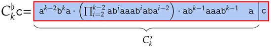
Figure 15. Introducing the Lyndon word $C_k^{♭}$$\mathtt{c}$ studied in Section 7.2.2.

Lemma 59.

$C_k^{♭}\mathtt{c}$ is a Lyndon word.

Proof. 

The longest run of $\mathtt{a}$ has a length of $k-2$, which is a prefix of $C_k^{♭}\mathtt{c}$ itself having prefix ${\mathtt{a}}^{k-2}\mathtt{b}$. Thus, $C_k^{♭}\mathtt{c}$ is a Lyndon word. □

Thus, we prove $\rho \left(C_k^{♭}\mathtt{c}\right)$ using the $\mathcal{M}\left(C_k^{♭}\mathtt{c}\right)$ as we did above.

Lemma 60.

$\beta ({\mathtt{a}}^{k-2}\mathtt{b},C_k^{♭}\mathtt{c})=\mathtt{c}.$

Proof. 

The first conjugate in $\mathcal{M}\left(C_k^{♭}\mathtt{c}\right)$ is ${\mathtt{a}}^{k-2}{\mathtt{b}}^k\mathtt{a}{P}_2\cdots \mathtt{c}$. The first conjugate in lexicographic order must start with the longest run of $\mathtt{a}$s. By the definition of $C_k^{♭}$, the longest run of $\mathtt{a}$ has length $k-2$, and it is obtained by concatenating the suffix ${\mathtt{a}}^{k-3}$ of $R_{k-1}$ with $Q_k$, which is preceded by a $\mathtt{c}$. □

Lemma 61.

$\beta ({\mathtt{a}}^i\mathtt{b},C_k^{♭}\mathtt{c})={\mathtt{ba}}^{k-2-i}$ for all $i\in [4..k-3]$.

Proof. 

All conjugates in $\mathcal{M}\left(C_k^{♭}\mathtt{c}\right)$ starting with the prefix ${\mathtt{a}}^i\mathtt{b}$ for any $i\in [4..k-3]$ are given below.

$$\begin{array}{c}\hfill {\mathtt{a}}^{i-1}{P}_{i+2}\cdots \mathtt{b}<{\mathtt{a}}^{i-1}{P}_{i+3}\cdots \mathtt{a}<\cdots <{\mathtt{a}}^{i-1}{P}_{k-1}\cdots \mathtt{a}<{\mathtt{a}}^{i-1}{Q}_k\cdots \mathtt{a}.\end{array}$$

For all $i\in [4..k-3]$, the factor ${\mathtt{a}}^i\mathtt{b}$ can only be obtained, for all $j\in [i+2..k-1]$, by concatenating the suffix ${\mathtt{a}}^{i-1}$ of $E_{j-1}$, with the prefix ab of $P_j$, or by concatenating suffix ${\mathtt{a}}^{k-3}$ of $R_{k-1}$ with the prefix $\mathtt{ab}$ of $Q_k$. We can sort these conjugates according to the lexicographic order of ${\bigcup }_{j=i}^{k-3}\left\{{\mathtt{a}}^{i-1}{P}_{j+2}\right\}\cup \left\{{\mathtt{a}}^{i-1}{Q}_k\right\}$. Note that all these conjugates end with an $\mathtt{a}$, with the exception of the conjugate starting with ${\mathtt{a}}^{i-1}{P}_{i+2}$, since it is here the only occurrence of ${\mathtt{ba}}^i\mathtt{b}$ can be found. □

Lemma 62.

$\beta (\mathtt{aaab},C_k^{♭}\mathtt{c})=\mathtt{bbbbb}{\left(\mathtt{ab}\right)}^{k-6}\mathtt{a}$.

Proof. 

The conjugates in $\mathcal{M}\left(C_k^{♭}\mathtt{c}\right)$ starting with the prefix $\mathtt{aaab}$ are

$$\begin{array}{cc}\hfill \mathtt{aa}{E}_2\cdots \mathtt{b}& <\mathtt{aa}{E}_3\cdots \mathtt{b}<\mathtt{aa}{E}_4\cdots \mathtt{b}<\mathtt{aa}{P}_5\cdots \mathtt{b}<\mathtt{aa}{E}_5\cdots \mathtt{b}\hfill \\ & <\mathtt{aa}{P}_6\cdots \mathtt{a}<\mathtt{aa}{E}_6\cdots \mathtt{b}<\cdots <\mathtt{aa}{P}_{k-2}\cdots \mathtt{a}<\mathtt{aa}{R}_{k-1}\cdots \mathtt{b}<\mathtt{aa}{Q}_k\cdots \mathtt{a}.\hfill \end{array}$$

These conjugates are obtained from the following cases.

Case 1:

  concatenating suffix $\mathtt{aa}$ of $P_i$ with prefix $\mathtt{ab}$ of $E_i$, for all $i\in [2..k-2]$ or with $R_{k-1}$ if $i=k-1$,

Case 2:

  concatenating suffix $\mathtt{aa}$ of $E_{i-1}$ with prefix $\mathtt{ab}$ of $P_i$ for all $i\in [5..k-1]$,

Case 3:

  concatenating suffix $\mathtt{aa}$ of $R_{k-1}$ with prefix $\mathtt{ab}$ of $Q_k$.

All these conjugates starting with $\mathtt{aaab}$ are sorted according to the lexicographic order of the words in ${\bigcup }_{i=2}^4\left\{\mathtt{aa}{E}_i\right\}\cup \{\mathtt{aa}{P}_5·\mathtt{aa}{E}_5\}\cup {\bigcup }_{i=6}^{k-2}\{\mathtt{aa}{P}_i·\mathtt{aa}{E}_i\}\cup \{\mathtt{aa}{P}_{k-1}·\mathtt{aa}{R}_{k-1}\}\cup \left\{\mathtt{aa}{Q}_k\right\}$. Note that all the conjugates starting either with $\mathtt{aa}{P}_i$, for all $i\in [6..k-1]$ of Case 2, or Case 3 end with $\mathtt{a}$. On the other hand, the conjugates starting either with $\mathtt{aa}{P}_5$ of Case 2 or Case 1 end with a $\mathtt{b}$. □

Lemma 63.

$\beta (\mathtt{aab},C_k^{♭}\mathtt{c})={\mathtt{baaba}}^{2k-8}.$

Proof. 

The conjugates in $\mathcal{M}\left(C_k^{♭}\mathtt{c}\right)$ that starts with the prefix $\mathtt{aab}$ are

$$\begin{array}{cc}\hfill \mathtt{a}{P}_2\cdots \mathtt{b}& <\mathtt{a}{E}_2\cdots \mathtt{a}<\mathtt{a}{E}_3\cdots \mathtt{a}<\mathtt{a}{P}_4\cdots \mathtt{b}<\mathtt{a}{E}_4\cdots \mathtt{a}<\mathtt{a}{P}_5\cdots \mathtt{a}\hfill \\ & <\mathtt{a}{E}_5\cdots \mathtt{a}<\cdots <\mathtt{a}{P}_{k-2}\cdots \mathtt{a}<\mathtt{a}{E}_{k-2}\cdots \mathtt{a}<\mathtt{a}{P}_{k-1}\cdots \mathtt{a}<\mathtt{a}{R}_{k-1}\cdots \mathtt{a}\hfill \\ & <\mathtt{a}{Q}_k\cdots \mathtt{a}.\hfill \end{array}$$

Each of the conjugates starting with $\mathtt{aaab}$ from Lemma 62 induces a conjugate starting with $\mathtt{aab}$, obtained by shifting one character on the left $\mathtt{a}$. It follows that all of these conjugates end with $\mathtt{a}$. The other conjugates starting with $\mathtt{aab}$ are the ones obtained by concatenating suffix $\mathtt{a}$ of $Q_k$ with $\mathtt{ab}$ of $P_2$, and another is obtained by concatenating suffix $\mathtt{a}$ of $E_3$ with $\mathtt{ab}$ of $P_4$. Moreover, both conjugates end with a $\mathtt{b}$. We prove our claim by sorting the conjugates according to the lexicographic order of the words in $\{\mathtt{a}{P}_2·\mathtt{a}{E}_2·\mathtt{a}{E}_3\}\cup {\bigcup }_{i=4}^{k-2}\{\mathtt{a}{P}_i·\mathtt{a}{E}_i\}\cup \{\mathtt{a}{P}_{k-1}·\mathtt{a}{R}_{k-1}\}\cup \left\{\mathtt{a}{Q}_k\right\}$. □

Lemma 64.

$\beta (\mathtt{ab},C_k^{♭}\mathtt{c})={\mathtt{b}}^{k-3}{\mathtt{aaba}}^{2k-6}$.

Proof. 

In $\mathcal{M}\left(C_k^{♭}\mathtt{c}\right)$, the conjugates which start with prefix $\mathtt{ab}$ are

$$\begin{array}{cc}\hfill {\mathtt{aba}}^{k-4}{P}_{k-1}\cdots \mathtt{b}& <{\mathtt{aba}}^{k-5}{P}_{k-2}\cdots \mathtt{b}<\cdots <\mathtt{ab}{P}_3\cdots \mathtt{b}\hfill \\ & <P_2\cdots \mathtt{a}<E_2\cdots \mathtt{a}<P_3\cdots \mathtt{b}<E_3\cdots \mathtt{a}\hfill \\ & <P_4\cdots \mathtt{a}<E_4\cdots \mathtt{a}<\cdots <P_{k-2}\cdots \mathtt{a}<E_{k-2}\cdots \mathtt{a}\hfill \\ & <P_{k-1}\cdots \mathtt{a}<R_{k-1}\cdots \mathtt{a}<Q_k\cdots \mathtt{a}.\hfill \end{array}$$

For all two distinct integers $i,i^{\prime }$ with $i>i^{\prime }\ge 0$, we have ${\mathtt{aba}}^i\mathtt{b}<{\mathtt{aba}}^{i^{\prime }}\mathtt{b}$. Thus, the first conjugate in lexicographic order starting with $\mathtt{ab}$ is the one which is followed by the longest run of $\mathtt{a}$s. The smallest of these conjugates can be found by concatenating the suffix ${\mathtt{aba}}^{k-4}$ of $E_{k-2}$ with the prefix $\mathtt{ab}$ of $P_{k-1}$, followed by the suffix ${\mathtt{aba}}^{i-3}$ of $E_{i-1}$ concatenated with the prefix $\mathtt{ab}$ of $P_i$, for all $i\in [3..k-2]$ all taken in decreasing order. By construction of $E_i$, for all $i\in [2..k-2]$, these conjugates must end with a $\mathtt{b}$. The remaining conjugates starting with $\mathtt{ab}$ are exactly those conjugates having as prefix either $P_i$ for all $i\in [2..k-1]$ and $E_{i^{\prime }}$ for all $i^{\prime }\in [2..k-2]$ or $R_{k-1}$ and $Q_k$. Note that all of these conjugates are obtained by shifting one character on the left $\mathtt{a}$ from the conjugates starting with $\mathtt{aab}$ from Lemma 63, with the exception of one starting with $P_3$. It follows that the latter ends with a $\mathtt{b}$, while all the other conjugates end with an $\mathtt{a}$. □

Lemma 65.

$\beta (\mathtt{ac},C_k^{♭}\mathtt{c})=\mathtt{b}.$

Proof. 

In $\mathcal{M}\left(C_k^{♭}\mathtt{c}\right)$, the conjugate that starts with prefix $\mathtt{ac}$ is ${\mathtt{aca}}^{k-3}{Q}_k\cdots \mathtt{b}$. The lexicographic order of $\mathtt{c}$ is larger than $\mathtt{b}$ or $\mathtt{a}$, so the prefix $\mathtt{ac}$ is also larger than the prefix $\mathtt{ab}$. $\mathtt{ac}$ is obtained from $R_{k-1}$, preceded by a $\mathtt{b}$. □

Lemma 66.

$\beta (\mathtt{ba},C_k^{♭}\mathtt{c})={\mathtt{a}}^{k-6}{\mathtt{bbbab}}^{k-4}{\mathtt{ab}}^{k-3}\mathtt{ab}.$

Proof. 

In $\mathcal{M}\left(C_k^{♭}\mathtt{c}\right)$, the conjugates starting with the prefix $\mathtt{ba}$ are

$$\begin{array}{cc}\hfill {\mathtt{ba}}^{k-4}{P}_{k-1}\cdots \mathtt{a}& <{\mathtt{ba}}^{k-5}{P}_{k-2}\cdots \mathtt{a}<\cdots <\mathtt{baaa}{P}_6\cdots \mathtt{a}\hfill \\ & <\mathtt{baa}{E}_2\cdots \mathtt{b}<\mathtt{baa}{E}_3\cdots \mathtt{b}<\mathtt{baa}{E}_4\cdots \mathtt{b}<\mathtt{baa}{P}_5\cdots \mathtt{a}\hfill \\ & <\mathtt{baa}{E}_5\cdots \mathtt{b}<\mathtt{baa}{E}_6\cdots \mathtt{b}<\cdots <\mathtt{baa}{R}_{k-1}\cdots \mathtt{b}\hfill \\ & <\mathtt{ba}{P}_2\cdots \mathtt{b}<\mathtt{ba}{P}_4\cdots \mathtt{a}\hfill \\ & <{\mathtt{baba}}^{k-4}{P}_{k-1}\cdots \mathtt{b}<{\mathtt{baba}}^{k-5}{P}_{k-2}\cdots \mathtt{b}<\cdots <\mathtt{bab}{P}_3\cdots \mathtt{b}\hfill \\ & <\mathtt{b}{P}_3\cdots \mathtt{a}<{\mathtt{baca}}^{k-3}{Q}_k\cdots \mathtt{b}.\hfill \end{array}$$

One can notice that we have as many circular occurrences of $\mathtt{ba}$ as the number of maximal runs of $\mathtt{b}$s in $M\left(C_k^{♭}\mathtt{c}\right)$. The conjugates are obtained from the cases below.

Case 1:

  one run of $\mathtt{b}$s in $P_i$, for all $i\in [2..k-1]$,

Case 2:

  two runs in $E_i$ for all $i\in [2..k-2]$,

Case 3:

  one run in $Q_k$,

Case 4:

  one run in $R_{k-1}$.

For Case 1, we have one conjugate starting with $\mathtt{baa}{E}_i$ for each $i\in [2..k-1]$. Since each run of $\mathtt{b}$s within each word from ${\bigcup }_{i=2}^{k-1}\left\{P_i\right\}$ is of length of at least 2, all conjugates in Case 1 end with a $\mathtt{b}$.

For Case 2, with integer $i\in [2..k-2]$, we can distinguish between two subcases based on where $\mathtt{ba}$ starts:

Case 2 (a):

  a first run of $\mathtt{ba}$ in $E_i$, which has a prefix of ${\mathtt{baba}}^{i-2}{P}_{i+1}$ for all $i\in [2..k-2]$,

Case 2 (b):

  a second run of $\mathtt{ba}$ in $E_i$, which has a prefix of ${\mathtt{ba}}^{i-2}{P}_{i+1}$ for all $i\in [2..k-2]$.

• Similarly to Case 1, all the conjugates in Case 2 (a) end with a $\mathtt{b}$.
• Each conjugate in Case 2 (b) is obtained by shifting two characters on the right each conjugate in Case 2 (a). Therefore, all of these conjugates end with an $\mathtt{a}$.
• For Case 3, the conjugate starting with $\mathtt{ba}$ in $Q_k$ has $\mathtt{ba}{P}_2$ as a prefix, and it is preceded by a $\mathtt{b}$.
• For Case 4, $\mathtt{ba}$ in $R_{k-1}$ has ${\mathtt{baca}}^{k-3}$ as a prefix, and it is preceded by a $\mathtt{b}$.
• Observe that only for Case 2 (b) we have conjugates starting with $\mathtt{baaaa}$. Hence, the first conjugate in lexicographic order is the one starting with ${\mathtt{ba}}^{k-4}{P}_{k-1}$ followed by ${\mathtt{ba}}^{k-5}{P}_{k-2}<\cdots <\mathtt{baaa}{P}_6$.
• Among the remaining conjugates, those having prefix $\mathtt{baaa}$ either start with $\mathtt{baa}{P}_5$ from Case 2 (b) or $\mathtt{baa}{E}_i$ from Case 1 for all $i\in [2..k-1]$. Thus, we can sort them according to the order of the words in ${\bigcup }_{i=2}^4\left\{\mathtt{baa}{E}_i\right\}\cup \left\{\mathtt{baa}{P}_5\right\}\cup {\bigcup }_{i=5}^{k-2}\left\{\mathtt{baa}{E}_i\right\}$. Then, the remaining conjugates with prefix $\mathtt{baa}$ are those starting with $\mathtt{ba}{P}_2$ from Case 3 and $\mathtt{ba}{P}_4$ from Case 2 (b).

Finally, we focus on the conjugates from Case 2 (a). These conjugates are sorted according to the length of the run of $\mathtt{a}$s following the common prefix $\mathtt{bab}$. The last conjugates left are the one starting with $\mathtt{b}{P}_3$ from Case 2 (b). and the one starting with ${\mathtt{baca}}^{k-3}$ from Case 4. These conjugates are lexicographically organized and are greater than any other cases, and therefore we analyzed all conjugates. □

Lemma 67.

$\beta ({\mathtt{b}}^i\mathtt{a},C_k^{♭}\mathtt{c})={\mathtt{ab}}^{2k-2i-2}\mathtt{ab}$ for all $i\in [2..k-2]$.

Proof. 

In $\mathcal{M}\left(C_k^{♭}\mathtt{c}\right)$, the conjugates starting with ${\mathtt{b}}^i\mathtt{a}$ for all $i\in [2..k-2]$ are

$$\begin{array}{cc}\hfill {\mathtt{b}}^i\mathtt{aa}{E}_i\cdots \mathtt{a}& <{\mathtt{b}}^i\mathtt{aa}{E}_{i+1}\cdots \mathtt{b}<{\mathtt{b}}^i\mathtt{aa}{E}_{i+2}\cdots \mathtt{b}<\cdots <{\mathtt{b}}^i\mathtt{aa}{R}_{k-1}\cdots \mathtt{b}\hfill \\ & <{\mathtt{b}}^i\mathtt{a}{P}_2\cdots \mathtt{b}<{\mathtt{b}}^i{\mathtt{aba}}^{k-4}{P}_{k-1}\cdots \mathtt{b}<\cdots <{\mathtt{b}}^i{\mathtt{aba}}^{i-1}{P}_{i+2}\cdots \mathtt{b}\hfill \\ & <{\mathtt{b}}^i{\mathtt{aba}}^{i-2}{P}_{i+1}\cdots \mathtt{a}<{\mathtt{b}}^i{\mathtt{aca}}^{k-3}{Q}_k\cdots \mathtt{b}.\hfill \end{array}$$

All runs of $\mathtt{b}$s of length of at least $i\in [2..k-2]$ are obtained from the cases below.

Case 1:

  suffix ${\mathtt{b}}^i\mathtt{aa}$ in $P_j$, for all $j\in [i..k-1]$

Case 2:

  ${\mathtt{b}}^i{\mathtt{aba}}^{j-2}$ in $E_j$ for all $j\in [i..k-2]$,

Case 3:

  ${\mathtt{b}}^i\mathtt{a}$ in $Q_k$,

Case 4:

  ${\mathtt{b}}^i{\mathtt{aca}}^{k-3}$ in $R_{k-1}$.

• Consider the four cases separately. The conjugate starting within $P_j$ (Case 1) has as prefix ${\mathtt{b}}^i\mathtt{aa}{E}_j$ if only $j\in [i..k-2]$ or ${\mathtt{b}}^i\mathtt{aa}{R}_{k-1}$ if $j=k-1$.
• And for all $j\in [i..k-2]$, the conjugate starting within $E_j$ (Case 2) has as prefix ${\mathtt{b}}^i{\mathtt{aba}}^{j-2}{P}_{j+1}$.
• In addition, the conjugate starting within $Q_k$ (Case 3) has as prefix ${\mathtt{b}}^i\mathtt{a}{P}_2$.
• Finally, the conjugate that begins within $R_{k-1}$ (Case 4) has as prefix ${\mathtt{b}}^i{\mathtt{aca}}^{k-3}$.

By construction, we have all the conjugates from Case 1 sorted according to the lexicographic order of the words in ${\bigcup }_{j=i}^{k-2}\left\{{\mathtt{b}}^i\mathtt{aa}{E}_j\right\}\cup \left\{{\mathtt{b}}^i\mathtt{aa}{R}_{k-1}\right\}$; then, we have the conjugate from Case 3. Then, the conjugates of Case 2 are sorted according to the decreasing length of the run of $\mathtt{a}$s following the common prefix ${\mathtt{b}}^i\mathtt{ab}$. Finally, the conjugate of Case 4 follows. Moreover, note that only when the run of $\mathtt{b}$s is exactly of length i the conjugate ends with an $\mathtt{a}$. Thus, only the conjugates ending with an $\mathtt{a}$ are those starting within $P_i$ and $E_i$, i.e., those with prefix ${\mathtt{b}}^i\mathtt{aa}{E}_i$ and ${\mathtt{b}}^i{\mathtt{aba}}^{i-2}{P}_{i+1}$. □

Lemma 68.

$\beta ({\mathtt{b}}^{k-1}\mathtt{a},C_k^{♭}\mathtt{c})=\mathtt{aba}.$

Proof. 

In $\mathcal{M}\left(C_k^{♭}\mathtt{c}\right)$, there are exactly three conjugates that start with prefix ${\mathtt{b}}^{k-1}\mathtt{a}$. These are

$$\begin{array}{c}\hfill {\mathtt{b}}^{k-1}{\mathtt{aaab}}^{k-1}{\mathtt{aca}}^{k-3}{Q}_k\cdots \mathtt{a}<{\mathtt{b}}^{k-1}\mathtt{a}{P}_2\cdots \mathtt{b}<{\mathtt{b}}^{k-1}{\mathtt{aca}}^{k-3}{Q}_k\cdots \mathtt{a}.\end{array}$$

Observe that the only conjugates with prefix ${\mathtt{b}}^{k-1}\mathtt{a}$ start within $P_{k-1}$, $Q_k$, and $R_{k-1}$. These conjugates have prefixes of, respectively, ${\mathtt{b}}^{k-1}{R}_{k-1}$, ${\mathtt{b}}^{k-1}\mathtt{a}{P}_2$, ${\mathtt{b}}^{k-1}{\mathtt{aca}}^{k-3}{Q}_k$. One can see that these conjugates taken in this order are already sorted, and only the conjugate starting within $Q_k$ ends with $\mathtt{b}$, while the other two end with $\mathtt{a}$. □

Lemma 69.

$\beta ({\mathtt{b}}^k\mathtt{a},C_k^{♭}\mathtt{c})=\mathtt{a}.$

Proof. 

In $\mathcal{M}\left(C_k^{♭}\mathtt{c}\right)$, only one conjugate starts with a prefix of ${\mathtt{b}}^k\mathtt{a}$ and it is ${\mathtt{b}}^k\mathtt{a}{P}_2\cdots \mathtt{a}$. The only occurrence of ${\mathtt{b}}^k\mathtt{a}$ is within $Q_k$, preceded by $\mathtt{a}$. □

Lemma 70.

$\beta (\mathtt{c},C_k^{♭}\mathtt{c})=\mathtt{a}.$

Proof. 

The last conjugate in $\mathcal{M}\left(C_k^{♭}\mathtt{c}\right)$ that starts with prefix $\mathtt{c}$ is ${\mathtt{ca}}^{k-3}{Q}_k\cdots \mathtt{a}$. The last conjugate in lexicographic order that starts with $\mathtt{c}$ occurs in $R_{k-1}$. Since $\mathtt{c}$ is preceded by an $\mathtt{a}$, it ends with $\mathtt{a}$. □

The following theorem puts the above lemmas together.

Theorem 13.

$\rho \left(C_k^{♭}\mathtt{c}\right)=8k-13$, cf. Table 16. The BBWT of $C_k^{♭}\mathtt{c}$ is BBWT($C_k^{♭}\mathtt{c}$) = ${\prod }_{i=2}^{k-1}\beta \left({\mathtt{a}}^{k-i}\mathtt{b}\right)·\beta \left(\mathtt{ac}\right)·{\prod }_{i=1}^k\beta \left({\mathtt{b}}^i\mathtt{a}\right)·\beta \left(\mathtt{c}\right)$.

Table 16. Classification of the number of runs obtained in Theorem 13. The total number of runs is $8k-13$.

BWT of ${\mathit{C}}_{\mathit{k}}^{♭}\mathtt{c}$	Runs
$\beta \left({\mathtt{a}}^{k-2}\mathtt{b}\right)=\mathtt{c}$	1
$\beta \left({\mathtt{a}}^i\mathtt{b}\right)={\mathtt{ba}}^{k-2-i}$ for all $i\in [4..k-3]$	$2k-12$
$\beta \left(\mathtt{aaab}\right)=\mathtt{bbbbb}{\left(\mathtt{ab}\right)}^{k-6}\mathtt{a}$	$2k-10$
$\beta \left(\mathtt{aab}\right)={\mathtt{baaba}}^{2k-8}$	4
$\beta \left(\mathtt{ab}\right)={\mathtt{b}}^{k-3}{\mathtt{aaba}}^{2k-6}$	4
$\beta \left(\mathtt{ac}\right)=\mathtt{b}$	1
$\beta \left(\mathtt{ba}\right)={\mathtt{a}}^{k-6}{\mathtt{bbbab}}^{k-4}{\mathtt{ab}}^{k-3}\mathtt{ab}$	8
$\beta \left({\mathtt{b}}^i\mathtt{a}\right)={\mathtt{ab}}^{2k-2i-2}\mathtt{ab}$ for all $i\in [2..k-2]$	$4k-12$
$\beta \left({\mathtt{b}}^{k-1}\mathtt{a}\right)=\mathtt{aba}$	3
$\beta \left({\mathtt{b}}^k\mathtt{a}\right)=\mathtt{a}$	1 but, when merged, 0
$\beta \left(\mathtt{c}\right)=\mathtt{a}$	1 but, when merged, 0

Proof. 

Every conjugate contributing a character to $\beta \left({\mathtt{a}}^i\mathtt{b}\right)$ is smaller than any conjugate of $\beta \left({\mathtt{a}}^{i^{\prime }}\mathtt{b}\right)$, for all $1\le i^{\prime }\le i\le k-2$. Symmetrically, every conjugate contributing a character to $\beta \left({\mathtt{b}}^j\mathtt{a}\right)$ is greater than any conjugate of $\beta \left({\mathtt{b}}^{j^{\prime }}\mathtt{a}\right)$, for every $1\le j^{\prime }\le j\le k$. Since we considered all the disjoint ranges of conjugates of $C_k\mathtt{c}$ based on their common prefix, ${\prod }_{i=2}^{k-1}\beta \left({\mathtt{a}}^{k-i}\mathtt{b}\right)·\beta \left(\mathtt{ac}\right)·{\prod }_{i=1}^k\beta \left({\mathtt{b}}^i\mathtt{a}\right)·\beta \left(\mathtt{c}\right)$ is the BBWT and BWT of $C_k^{♭}\mathtt{c}$.

With the structure of BWT($C_k^{♭}\mathtt{c}$), we can easily derive its number of runs. The word ${\prod }_{i=2}^{k-4}\beta \left({\mathtt{a}}^{k-i}\mathtt{b}\right)$ has exactly $2k-11$ runs: we start with 1 run from $\beta \left({\mathtt{a}}^{k-2}\mathtt{b}\right)=\mathtt{c}$, and then concatenating each from $\beta \left({\mathtt{a}}^{k-3}\mathtt{b}\right)$ to $\beta \left({\mathtt{a}}^4\mathtt{b}\right)$ adds 2 runs each. By counting, we observe that $\beta \left(\mathtt{aaab}\right),\beta \left(\mathtt{aab}\right),$ and $\beta \left(\mathtt{ab}\right)$ contribute $2k-10$, 4, and 4 runs, respectively. The boundaries between these words do not merge. The conjugates in $\beta \left(\mathtt{ac}\right)$ and $\beta \left(\mathtt{ba}\right)$ contribute with 1 and 8 runs each. The remaining parts of the BWT ${\prod }_{i=2}^k\beta \left({\mathtt{b}}^i\mathtt{a}\right)$ contribute $4(k-3)+3$ runs: we start adding 4 runs each by concatenating each $\beta \left(\mathtt{bba}\right)$ to $\beta \left({\mathtt{b}}^{k-2}\mathtt{a}\right)$. And $\beta \left({\mathtt{b}}^{k-1}\mathtt{a}\right)$ adds 3 runs. $\beta \left({\mathtt{b}}^k\mathtt{a}\right)$ and $\beta \left(\mathtt{c}\right)$ do not add new runs, as they consist only of an $\mathtt{a}$ that merges with the previous one. The last part $\beta \left(\mathtt{c}\right)$ contributes one run. In total, we have $2k-11+2k-10+4+4+1+8+4k-12+3=8k-13$, and the claim holds. □

8. Conclusions

In this article, we analyzed the sensitivity of the Burrows–Wheeler Transform (BWT) and its bijective variant (BBWT) to single-character edits. We extended previous work on the BWT by a four-character alphabet setting and an alphabet reordering. Our findings reveal that BWT and BBWT exhibit similar sensitivity characteristics, with compression size changes that can follow a multiplicative logarithmic or additive square-root growth. These insights clarify that the BWT and BBWT are not robust repetitiveness measures, which is a crucial property for data compression applications. As future work, we would like to find positions in a word for which we can predict the compression size changes when editing that position. That would allow us to design algorithms to improve the compression power of BWT/BBWT by editing the word in a way that minimizes the compression size changes.

References

- Burrows, M.; Wheeler, D.J. A Block Sorting Lossless Data Compression Algorithm; Technical Report 124; Digital Equipment Corporation: Palo Alto, CA, USA, 1994. [Google Scholar]
- Ferragina, P.; Manzini, G. Opportunistic Data Structures with Applications. In Proceedings of the 41st Annual Symposium on Foundations of Computer Science, Redondo Beach, CA, USA, 12–14 November 2000; pp. 390–398. [Google Scholar] [CrossRef]
- Gagie, T.; Navarro, G.; Prezza, N. Optimal-Time Text Indexing in BWT-runs Bounded Space. In Proceedings of the Twenty-Ninth Annual ACM-SIAM Symposium on Discrete Algorithms, New Orleans, LA, USA, 7–10 January 2018; pp. 1459–1477. [Google Scholar] [CrossRef]
- Gagie, T.; Navarro, G.; Prezza, N. Fully Functional Suffix Trees and Optimal Text Searching in BWT-Runs Bounded Space. J. ACM 2020, 67, 2:1–2:54. [Google Scholar] [CrossRef]
- Bertram, N.; Fischer, J.; Nalbach, L. Move-r: Optimizing the r-index. In Proceedings of the 22nd International Symposium on Experimental Algorithms (SEA 2024), Vienna, Austria, 23–26 July 2024; Volume 301, pp. 1:1–1:19. [Google Scholar] [CrossRef]
- Cobas, D.; Gagie, T.; Navarro, G. A Fast and Small Subsampled R-Index. In Proceedings of the 32nd Annual Symposium on Combinatorial Pattern Matching (CPM 2021), Wrocław, Poland, 5–7 July 2021; Volume 191, pp. 13:1–13:16. [Google Scholar] [CrossRef]
- Arakawa, Y.; Navarro, G.; Sadakane, K. Bi-Directional r-Indexes. In Proceedings of the 33rd Annual Symposium on Combinatorial Pattern Matching (CPM 2022), Prague, Czech Republic, 27–29 June 2022; Volume 223, pp. 11:1–11:14. [Google Scholar] [CrossRef]
- Shivakumar, V.S.; Ahmed, O.Y.; Kovaka, S.; Zakeri, M.; Langmead, B. Sigmoni: Classification of nanopore signal with a compressed pangenome index. Bioinformatics 2024, 40, i287–i296. [Google Scholar] [CrossRef]
- Langmead, B.; Salzberg, S.L. Fast gapped-read alignment with Bowtie 2. Nat. Methods 2012, 9, 357–359. [Google Scholar] [CrossRef] [PubMed]
- Li, R.; Yu, C.; Li, Y.; Lam, T.W.; Yiu, S.; Kristiansen, K.; Wang, J. SOAP2: An improved ultrafast tool for short read alignment. Bioinformatics 2009, 25, 1966–1967. [Google Scholar] [CrossRef] [PubMed]
- Ferragina, P.; Manzini, G.; Muthukrishnan, S.M. The Burrows–Wheeler Transform: Ten Years Later; DIMACS: Piscataway, NJ, USA, 2004. [Google Scholar]
- Gagie, T.; Manzini, G.; Navarro, G.; Stoye, J. 25 Years of the Burrows–Wheeler Transform (Dagstuhl Seminar 19241). Dagstuhl Rep. 2019, 9, 55–68. [Google Scholar]
- Adjeroh, D.; Bell, T.; Mukherjee, A. The Burrows–Wheeler Transform: Data Compression, Suffix Arrays, and Pattern Matching; Springer: Berlin/Heidelberg, Germany, 2008. [Google Scholar]
- Gessel, I.M.; Reutenauer, C. Counting Permutations with Given Cycle Structure and Descent Set. J. Comb. Theory Ser. A 1993, 64, 189–215. [Google Scholar]
- Schindler, M. A fast block-sorting algorithm for lossless data compression. In Proceedings of the DCC ’97. Data Compression Conference, Snowbird, UT, USA, 25–27 March 1997; p. 469. [Google Scholar] [CrossRef]
- Mantaci, S.; Restivo, A.; Rosone, G.; Sciortino, M. An extension of the Burrows–Wheeler Transform. Theor. Comput. Sci. 2007, 387, 298–312. [Google Scholar] [CrossRef]
- Kufleitner, M. On Bijective Variants of the Burrows–Wheeler Transform. In Proceedings of the Prague Stringology Conference 2009 (PSC 2009), Prague, Czech Republic, 31 August–2 September 2009; pp. 65–79. [Google Scholar]
- Daykin, J.W.; Smyth, W.F. A bijective variant of the Burrows–Wheeler Transform using V-order. Theor. Comput. Sci. 2014, 531, 77–89. [Google Scholar] [CrossRef]
- Daykin, J.W.; Groult, R.; Guesnet, Y.; Lecroq, T.; Lefebvre, A.; Léonard, M.; Prieur-Gaston, É. Binary block order Rouen Transform. Theor. Comput. Sci. 2016, 656, 118–134. [Google Scholar] [CrossRef]
- Gil, J.Y.; Scott, D.A. A Bijective String Sorting Transform. arXiv 2012, arXiv:1201.3077. [Google Scholar] [CrossRef]
- Likhomanov, K.M.; Shur, A.M. Two Combinatorial Criteria for BWT Images. In Computer Science–Theory and Applications; Springer: Berlin/Heidelberg, Germany, 2011; Volume 6651, pp. 385–396. [Google Scholar] [CrossRef]
- Giuliani, S.; Lipták, Z.; Masillo, F.; Rizzi, R. When a dollar makes a BWT. Theor. Comput. Sci. 2021, 857, 123–146. [Google Scholar] [CrossRef]
- Giuliani, S.; Lipták, Z.; Masillo, F. When a Dollar in a Fully Clustered Word Makes a BWT. Ceur Workshop Proc. 2022, 3284, 122–135. [Google Scholar]
- Giuliani, S.; Inenaga, S.; Lipták, Z.; Romana, G.; Sciortino, M.; Urbina, C. Bit Catastrophes for the Burrows–Wheeler Transform. In Developments in Language Theory; Springer: Berlin/Heidelberg, Germany, 2023; Volume 13911, pp. 86–99. [Google Scholar] [CrossRef]
- Akagi, T.; Funakoshi, M.; Inenaga, S. Sensitivity of string compressors and repetitiveness measures. Inf. Comput. 2023, 291, 104999. [Google Scholar] [CrossRef]
- Lagarde, G.; Perifel, S. Lempel-Ziv: A “one-bit catastrophe” but not a tragedy. In Proceedings of the Twenty-Ninth Annual ACM-SIAM Symposium on Discrete Algorithms, New Orleans, LA, USA, 7–10 January 2018; pp. 1478–1495. [Google Scholar] [CrossRef]
- Ziv, J.; Lempel, A. A universal algorithm for sequential data compression. IEEE Trans. Inf. Theory 1977, 23, 337–343. [Google Scholar] [CrossRef]
- Ziv, J.; Lempel, A. Compression of individual sequences via variable-rate coding. IEEE Trans. Inf. Theory 1978, 24, 530–536. [Google Scholar] [CrossRef]
- Kempa, D.; Prezza, N. At the roots of dictionary compression: String attractors. In Proceedings of the 50th Annual ACM SIGACT Symposium on Theory of Computing, Los Angeles, CA, USA, 25–29 June 2018; pp. 827–840. [Google Scholar] [CrossRef]
- Navarro, G.; Ochoa, C.; Prezza, N. On the Approximation Ratio of Ordered Parsings. IEEE Trans. Inf. Theory 2021, 67, 1008–1026. [Google Scholar] [CrossRef]
- Nakashima, Y.; Köppl, D.; Funakoshi, M.; Inenaga, S.; Bannai, H. Edit and Alphabet-Ordering Sensitivity of Lex-Parse. In Proceedings of the 49th International Symposium on Mathematical Foundations of Computer Science (MFCS 2024), Bratislava, Slovakia, 26–30 August 2024; Volume 306, pp. 75:1–75:15. [Google Scholar] [CrossRef]
- Blumer, A.; Blumer, J.; Haussler, D.; Ehrenfeucht, A.; Chen, M.T.; Seiferas, J.I. The Smallest Automaton Recognizing the Subwords of a Text. Theor. Comput. Sci. 1985, 40, 31–55. [Google Scholar] [CrossRef]
- Fujimaru, H.; Nakashima, Y.; Inenaga, S. On Sensitivity of Compact Directed Acyclic Word Graphs. In Combinatorics on Words; Springer: Berlin/Heidelberg, Germany, 2023; Volume 13899, pp. 168–180. [Google Scholar] [CrossRef]
- Olbrich, J.; Ohlebusch, E.; Büchler, T. Generic Non-recursive Suffix Array Construction. ACM Trans. Algorithms 2024, 20, 18. [Google Scholar] [CrossRef]
- Bannai, H.; Kärkkäinen, J.; Köppl, D.; Piątkowski, M. Constructing and Indexing the Bijective and Extended Burrows–Wheeler Transform. Inf. Comput. 2024, 297, 1–30. [Google Scholar] [CrossRef]
- Badkobeh, G.; Bannai, H.; Köppl, D. Bijective BWT based Compression Schemes. In String Processing and Information Retrieval; Springer: Berlin/Heidelberg, Germany, 2024; Volume 14899, pp. 16–25. [Google Scholar] [CrossRef]
- Biagi, E.; Cenzato, D.; Lipták, Z.; Romana, G. On the Number of Equal-Letter Runs of the Bijective Burrows–Wheeler Transform. In Proceedings of the International Conference on Information and Communication Technology for Competitive Strategies (ICTCS), Jaipur, India, 8–9 December 2023; Volume 3587, pp. 129–142. [Google Scholar]
- Lyndon, R.C. On Burnside’s Problem. Trans. Am. Math. Soc. 1954, 77, 202–215. [Google Scholar]
- Chen, K.T.; Fox, R.H.; Lyndon, R.C. Free differential calculus, IV. The quotient groups of the lower central series. Ann. Math. 1958, 68, 81–95. [Google Scholar]
- Lothaire, M. Combinatorics on Words, 2nd ed.; Cambridge Mathematical Library, Cambridge University Press: Cambridge, UK, 1997. [Google Scholar]
- Saari, K. Lyndon words and Fibonacci numbers. J. Comb. Theory Ser. A 2014, 121, 34–44. [Google Scholar] [CrossRef]
- De Luca, A.; Mignosi, F. Some Combinatorial Properties of Sturmian Words. Theor. Comput. Sci. 1994, 136, 361–385. [Google Scholar] [CrossRef]
- Mantaci, S.; Restivo, A.; Sciortino, M. Burrows–Wheeler transform and Sturmian words. Inf. Process. Lett. 2003, 86, 241–246. [Google Scholar] [CrossRef]
- Christodoulakis, M.; Iliopoulos, C.S.; Ardila, Y.J.P. Simple Algorithm for Sorting the Fibonacci String Rotations. In Proceedings of the SOFSEM, Merin, Czech Republic, 21–27 January 2006; Volume 3831, pp. 218–225. [Google Scholar] [CrossRef]
- Séébold, P. Fibonacci Morphisms and Sturmian Words. Theor. Comput. Sci. 1991, 88, 365–384. [Google Scholar] [CrossRef]
- Giuliani, S.; Inenaga, S.; Lipták, Z.; Prezza, N.; Sciortino, M.; Toffanello, A. Novel Results on the Number of Runs of the Burrows–Wheeler-Transform. In Proceedings of the SOFSEM, Bolzano-Bozen, Italy, 25–29 January 2021; Volume 12607, pp. 249–262. [Google Scholar] [CrossRef]
- Boucher, C.; Cenzato, D.; Lipták, Z.; Rossi, M.; Sciortino, M. r-Indexing the eBWT. In Proceedings of the SPIRE, Lille, France, 4–6 October 2021; Volume 12944, pp. 3–12. [Google Scholar] [CrossRef]
Disclaimer/Publisher’s Note: The statements, opinions and data contained in all publications are solely those of the individual author(s) and contributor(s) and not of MDPI and/or the editor(s). MDPI and/or the editor(s) disclaim responsibility for any injury to people or property resulting from any ideas, methods, instructions or products referred to in the content. |
© 2025 by the authors. Licensee MDPI, Basel, Switzerland. This article is an open access article distributed under the terms and conditions of the Creative Commons Attribution (CC BY) license (https://creativecommons.org/licenses/by/4.0/).