Conditional Quantization for Uniform Distributions on Line Segments and Regular Polygons ^†

Abstract

Quantization for a Borel probability measure refers to the idea of estimating a given probability by a discrete probability with support containing a finite number of elements. If, in the quantization some of the elements in the support are preselected, then the quantization is called a conditional quantization. In this paper, we investigate the conditional quantization for the uniform distributions defined on the unit line segments and m-sided regular polygons, where $m\ge 3$, inscribed in a unit circle.

1. Introduction

The process of transformation of a continuous-valued signal into a discrete-valued one is called ‘quantization’. It has broad applications in engineering and technology. We refer to [1,2,3] for surveys on the subject and comprehensive lists of references to the literature; see also [4,5,6,7]. For mathematical treatment of quantization, one is referred to Graf–Luschgy’s book (see [6]). For some other recent papers on quantization. one can see [1,2,3,6,7,8,9,10,11,12,13,14,15,16,17,18]. Recently, Pandey and Roychowdhury introduced the concepts of constrained quantization and the conditional quantization (for example, see [19,20,21,22]). This paper deals with conditional quantization.

Definition 1. 

Let P be a Borel probability measure on ${\mathbb{R}}^2$ equipped with a Euclidean metric d induced by the Euclidean norm $\parallel ·\parallel$. Let $\beta \subset {\mathbb{R}}^2$ be given with $card(\beta )=\ell$ for some $\ell \in \mathbb{N}$. Then, for $n\in \mathbb{N}$ with $n\ge \ell$, the nth conditional quantization error for P with respect to the conditional set β is defined as

$$V_n:=V_n(P)=\underset{\alpha }{inf}\left\{\int \underset{a\in \alpha \cup \beta }{min}d{(x,a)}^{2}dP(x):\mathrm{card}(\alpha )\le n-\ell \right\},$$

(1)

where card$(A)$ represents the cardinality of the set A.

We assume that $\int d{(x,0)}^{2}dP(x)<\infty$ to make sure that the infimum in (1) exists (see [19]). For a finite set $\gamma \subset {\mathbb{R}}^2$ and $a\in \gamma$, by $M(a|\gamma )$ we denote the set of all elements in ${\mathbb{R}}^2$ that are nearest to a among all the elements in $\gamma$, i.e., $M(a|\gamma )=\{x\in {\mathbb{R}}^2:d(x,a)=\underset{b\in \gamma }{min}d(x,b)\}.$ $M(a|\gamma )$ is called the Voronoi region in ${\mathbb{R}}^2$ generated by $a\in \gamma$.

Definition 2. 

A set $\alpha \cup \beta$, where $P(M(b|\alpha \cup \beta ))>0$ for $b\in \beta$, for which the infimum in $V_n$ exists and contains no less than ℓ elements and no more than n elements is called a conditional optimal set of n-points for P with respect to the conditional set β.

Let $V_{n,r}(P)$ be a strictly decreasing sequence, and write $V_{\infty ,r}(P):=\underset{n\to \infty }{lim}{V}_{n,r}(P)$. Then, the number

$$\begin{array}{c}\hfill D(P):=\underset{n\to \infty }{lim}{\displaystyle \frac{2logn}{-log(V_n(P)-V_{\infty }(P))}}\end{array}$$

if it exists, is called the conditional quantization dimension of P and is denoted by $D(P)$. The conditional quantization dimension measures the speed at which the specified measure of the conditional quantization error converges as n tends to infinity. For any $\kappa >0$, the number

$$\underset{n\to \infty }{lim}{n}^{\frac{2}{\kappa }}(V_n(P)-V_{\infty }(P)),$$

if it exists, is called the κ-dimensional conditional quantization coefficient for P.

In this paper, we investigate the conditional quantization for uniform distributions on the unit line segments and on regular m-sided polygons, where $m\ge 3$, inscribed in a unit circle.

1.1. Delineation

In this paper, there are three sections in addition to the section that contains the basic preliminaries. First, we have proved Proposition 1. In Section 3, as a special case of Proposition 1, we explicitly determine the conditional optimal sets of n-points and the nth conditional quantization errors for a uniform distribution with two interior elements as the conditional set for all $n\ge 2$ on the interval $[0,1]$. In Section 4, as an extension of Proposition 1, we calculate the conditional optimal sets of n-points and the nth conditional quantization errors for $(k-1)$ uniformly distributed interior elements on the interval $[0,1]$. On the other hand, Section 5 is an application of Proposition 1. It deals with a uniform distribution defined on the boundary of a regular m-sided polygon. Let P be a uniform distribution defined on the boundary of a regular m-sided polygon inscribed in a unit circle. After the introduction of conditional quantization, we know that the quantization dimension and the quantization coefficient do not depend on the conditional set (see [21]). Using this scenario, in Section 5, we calculate the quantization coefficient for the uniform distribution P defined on the boundary of the regular m-sided polygon inscribed in the unit circle by calculating the conditional quantization coefficient for P with respect to the conditional set $\beta$, which consists of all the vertices of the regular polygon. In addition, we also give an explicit formula to calculate the conditional optimal sets of n-points and the nth conditional quantization errors for the uniform distribution P for all $n\ge m$, where m is the number of vertices of the m-sided polygon.

1.2. Motivation and Significance

Conditional quantization has recently been introduced by Pandey–Roychowdhury in [21]. It has significant interdisciplinary applications: for example, in radiation therapy of cancer treatment to find the optimal locations of n centers of radiation, where k centers for some $k<n$ of radiation are preselected, the conditional quantization technique can be used. There are many interesting open problems that can be investigated. The work in this paper is an advancement in this direction. In [23], when there is no conditional set, Hansen et al., in a proposition, first determined the optimal sets of n-means and the nth quantization errors for the probability distribution P defined on the boundary of a regular m-sided polygon, when n is of the form $n=mk$ for some $k\in \mathbb{N}$. Then, with the help of the proposition, they showed that the quantization coefficient for P exists and equals ${\displaystyle \frac{1}{3}}{m}^2{sin}^2{\displaystyle \frac{\pi }{m}}$, i.e.,

$$\underset{n\to \infty }{lim}{n}^2{V}_n(P)={\displaystyle \frac{1}{3}}{m}^2{sin}^2{\displaystyle \frac{\pi }{m}}.$$

In this paper, we have also calculated the quantization coefficient for the same uniform distribution P, but the work in this paper is much simpler than the work to calculate the quantization coefficient done by Hansen et al. in [23].

2. Preliminaries

For any two elements $(a,b)$ and $(c,d)$ in ${\mathbb{R}}^2$, we write

$$\rho ((a,b),(c,d)):={(a-c)}^2+{(b-d)}^2,$$

which gives the squared Euclidean distance between the two elements $(a,b)$ and $(c,d)$. Two elements p and q in an optimal set of n-points are called adjacent elements if they have a common boundary in their own Voronoi regions. Let e be an element on the common boundary of the Voronoi regions of two adjacent elements p and q in an optimal set of n-points. Since the common boundary of the Voronoi regions of any two elements is the perpendicular bisector of the line segment joining the elements, we have

$$\rho (p,e)-\rho (q,e)=0.$$

We call such an equation a canonical equation. Notice that any element $x\in \mathbb{R}$ can be identified as an element $(x,0)\in {\mathbb{R}}^2$. Thus,

$$\rho :\mathbb{R}\times {\mathbb{R}}^2\to [0,\infty )\mathrm{such}\mathrm{that}\rho (x,(a,b))={(x-a)}^2+b^2,$$

where $x\in \mathbb{R}$ and $(a,b)\in {\mathbb{R}}^2$, defines a nonnegative real-valued function on $\mathbb{R}\times {\mathbb{R}}^2$. On the other hand,

$$\rho :\mathbb{R}\times \mathbb{R}\to [0,\infty )\mathrm{be}\mathrm{such}\mathrm{that}\rho (x,y)={(x-y)}^2,$$

where $x,y\in \mathbb{R}$, defines a nonnegative real-valued function on $\mathbb{R}\times \mathbb{R}$.

Let P be a Borel probability measure on $\mathbb{R}$ that is uniform on its support the closed interval $[a,b]$. Then, the probability density function f for P is given by

$$f(x)=\left\{\begin{array}{cc}{\displaystyle \frac{1}{b-a}}& \mathrm{if}a\le x\le b,\\ 0& \mathrm{otherwise}.\end{array}\right.$$

Hence, we have $dP(x)=P(dx)=f(x)dx$ for any $x\in \mathbb{R}$, where d stands for differential.

Notation 1. 

Let α be a discrete set. Then, for a Borel probability measure μ and a set A, by $V(\mu ;\{\alpha ,A\})$, it is meant the distortion error for μ with respect to the set α over the set A, i.e.,

$$V(\mu ;\{\alpha ,A\}):={\int }_A\underset{a\in \alpha }{min}\rho {(x,a)}^{2}d\mu (x).$$

(2)

The following proposition is a generalized version of Proposition 2.1, Proposition 2.2, and Proposition 2.3 that appear in [21].

Proposition 1. 

Let P be a uniform distribution on the closed interval $[a,b]$ and $c,d\in [a,b]$ be such that $a<c<d<b$. For $n\in \mathbb{N}$ with $n\ge 2$, let ${\alpha }_n$ be a conditional optimal set of n-points for P with respect to the conditional set $\beta =\{c,d\}$ such that ${\alpha }_n$ contains k elements from the closed interval $[a,c]$, ℓ elements from the closed interval $[c,d],$ and m elements from the closed interval $[d,b]$ for some $k,\ell ,m\in \mathbb{N}$ with $k,m\ge 1$ and $\ell \ge 2$. Then, $k+\ell +m=n+2$,

$$\begin{array}{cc}\hfill {\alpha }_n\cap [a,c]& =\left\{a+{\displaystyle \frac{(2j-1)(c-a)}{2k-1}}:1\le j\le k\right\},\hfill \\ \hfill {\alpha }_n\cap [c,d]& =\left\{c+{\displaystyle \frac{j-1}{\ell -1}}(d-c):1\le j\le \ell \right\},\mathrm{and}\hfill \\ \hfill {\alpha }_n\cap [d,b]& =\left\{d+{\displaystyle \frac{2(j-1)(b-d)}{2m-1}}:1\le j\le m\right\}\hfill \end{array}$$

with the conditional quantization error

$$V_n:=V_{k,\ell ,m}(P)={\displaystyle \frac{1}{3(b-a)}}\left({\displaystyle \frac{{(c-a)}^3}{{(2k-1)}^2}}+{\displaystyle \frac{1}{4}}{\displaystyle \frac{{(d-c)}^3}{{(\ell -1)}^2}}+{\displaystyle \frac{{(b-d)}^3}{{(2m-1)}^2}}\right).$$

Proof. 

Notice that the element c in the conditional set $\beta$ is common to both the intervals $[a,c]$ and $[c,d]$, the element d in the conditional set $\beta$ is common to both the intervals $[c,d]$ and $[d,b]$, and so c and d are counted two times. Hence, $k+\ell +m=n+2$. We have

$$[a,b]:=\{t:a\le t\le b\}.$$

Let ${\alpha }_n$ be a conditional optimal set of n-points such that

$$\begin{array}{cc}\hfill \mathrm{card}({\alpha }_n\cap [a,c])& =k\mathrm{and}\mathrm{card}({\alpha }_n\cap [c,d])=\ell ,\mathrm{and}\hfill \\ \hfill \mathrm{card}({\alpha }_n\cap [d,b])& =m,\mathrm{where}k,m\ge 1\mathrm{and}\ell \ge 2.\hfill \end{array}$$

Then, we can write

$$\begin{array}{cc}\hfill {\alpha }_n\cap [a,c]& =\{a_1,a_2,\cdots ,a_k\}\mathrm{and}{\alpha }_n\cap [c,d]=\{c_1,c_2,\cdots ,c_{\ell }\}\mathrm{and}\hfill \\ \hfill {\alpha }_n\cap [d,b]& =\{d_1,d_2,\cdots ,d_m\},\hfill \end{array}$$

such that

$$a<a_1<a_2<\cdots <a_k=c=c_1<c_2<\cdots <c_{\ell }=d=d_1<d_2<\cdots <d_m<b.$$

We now prove the following claim.

Claim. $a_2-a_1=a_3-a_2=\cdots =a_k-a_{k-1}={\displaystyle \frac{a_k-a_1}{k-1}}={\displaystyle \frac{c-a_1}{k-1}}.$

Since there is no restriction on the locations of the elements $a_j$ for $1\le j\le k-1$, they must be the conditional expectations in their own Voronoi regions. Hence, we have

$$\begin{array}{cc}\hfill a_1& =E(X:X\in [a,{\displaystyle \frac{1}{2}}(a_1+a_2)]),\hfill \end{array}$$

(3)

$$\begin{array}{cc}\hfill a_i& =E(X:X\in [{\displaystyle \frac{a_{i-1}+a_i}{2}},{\displaystyle \frac{a_i+a_{i+1}}{2}}])\mathrm{for}2\le i\le k-2,\hfill \end{array}$$

(4)

$$\begin{array}{cc}\hfill a_{k-1}& =E(X:X\in [{\displaystyle \frac{a_{k-2}+a_{k-1}}{2}},c]).\hfill \end{array}$$

(5)

By (3), we have

$$a_1={\displaystyle \frac{{\int }_a^{\frac{1}{2}(a_1+a_2)}xdP}{{\int }_a^{\frac{1}{2}(a_1+a_2)}dP}}={\displaystyle \frac{{\int }_a^{\frac{1}{2}(a_1+a_2)}xf(x)dx}{{\int }_a^{\frac{1}{2}(a_1+a_2)}f(x)dx}}={\displaystyle \frac{1}{4}}\left(2a+a_1+a_2\right).$$

Similarly, by (4) for $2\le i\le k-2$, we have

$$a_i={\displaystyle \frac{1}{4}}(a_{i-1}+2a_i+a_{i+1}),$$

and by (5), we deduce

$$a_{k-1}={\displaystyle \frac{1}{4}}(a_{k-2}+2a_{k-1}+a_k).$$

Combining all the expressions for $a_j$ for $1\le j\le k$, we have

$$a_2-a_1=a_3-a_2=\cdots =a_k-a_{k-1}={\displaystyle \frac{a_k-a_1}{k-1}}={\displaystyle \frac{c-a_1}{k-1}}.$$

(6)

Thus, the claim is true. Now, by (6), we have

$$\begin{array}{cc}\hfill a_2& =a_1+{\displaystyle \frac{c-a_1}{k-1}}=a_1+{\displaystyle \frac{c-a_1}{k-1}},\hfill \\ \hfill a_3& =a_2+{\displaystyle \frac{c-a_1}{k-1}}=a_1+2{\displaystyle \frac{c-a_1}{k-1}},\hfill \\ \hfill a_4& =a_3+{\displaystyle \frac{c-a_1}{k-1}}=a_1+3{\displaystyle \frac{c-a_1}{k-1}},\hfill \\ \hfill & \mathrm{and}\mathrm{so}\mathrm{on}.\hfill \end{array}$$

Thus, we have $a_j=a_1+(j-1){\displaystyle \frac{c-a_1}{k-1}}$ for $1\le j\le k$. The distortion error due to the elements ${\alpha }_n\cap [a,c]$ is given by

$$\begin{array}{cc}\hfill & V(P;\{{\alpha }_n\cap [a,c],[a,c]\})={\int }_{[a,c]}\underset{x\in {\alpha }_n\cap [a,c]}{min}\rho (t,x)dP\hfill \\ \hfill & ={\displaystyle \frac{1}{b-a}}\left({\int }_a^{{\displaystyle \frac{a_1+a_2}{2}}}\rho (t,a_1)dt+(k-2){\int }_{{\displaystyle \frac{a_1+a_2}{2}}}^{{\displaystyle \frac{a_2+a_3}{2}}}\rho (t,a_2)dt+{\int }_{{\displaystyle \frac{a_{k-1}+a_k}{2}}}^{a_k}\rho (t,a_k)dt\right)\hfill \\ \hfill & ={\displaystyle \frac{4a^3{(k-1)}^2-3a_1\left(4a^2{(k-1)}^2-c^2\right)+3a_1^2\left(4a{(k-1)}^2-c\right)-c^3+a_1^3\left(-4k^2+8k-3\right)}{12{(k-1)}^2(a-b)}},\hfill \end{array}$$

the minimum value of which is ${\displaystyle \frac{{(c-a)}^3}{3(b-a){(2k-1)}^2}}$ and it occurs when $a_1=a+{\displaystyle \frac{c-a}{2k-1}}$. Putting the values of $a_1$, we have

$$a_j=a+{\displaystyle \frac{(2j-1)(c-a)}{2k-1}}\mathrm{for}1\le j\le k\mathrm{with}V(P;\{{\alpha }_n\cap [a,c],[a,c]\})={\displaystyle \frac{{(c-a)}^3}{3(b-a){(2k-1)}^2}}.$$

Since the closed interval $[c,d]$ is a line segment and P is a uniform distribution, proceeding in the similar way as the proof given in the above claim, we have

$$c_2-c_1=c_3-c_2=\cdots =c_{\ell }-c_{\ell -1}={\displaystyle \frac{c_{\ell }-c_1}{\ell -1}}={\displaystyle \frac{d-c}{\ell -1}}$$

implying

$$\begin{array}{cc}\hfill c_2& =c_1+{\displaystyle \frac{d-c}{\ell -1}}=c+{\displaystyle \frac{d-c}{\ell -1}},\hfill \\ \hfill c_3& =c_2+{\displaystyle \frac{d-c}{\ell -1}}=c+{\displaystyle \frac{2(d-c)}{\ell -1}},\hfill \\ \hfill c_4& =c_3+{\displaystyle \frac{d-c}{\ell -1}}=c+{\displaystyle \frac{3(d-c)}{\ell -1}},\hfill \\ \hfill & \mathrm{and}\mathrm{so}\mathrm{on}.\hfill \end{array}$$

Thus, we have $c_j=c+{\displaystyle \frac{j-1}{\ell -1}}(d-c)$ for $1\le j\le \ell$. The distortion error contributed by the ℓ elements in the closed interval $[c,d]$ is given by

$$\begin{array}{cc}\hfill & V(P;\{{\alpha }_n\cap [c,d],[c,d]\})\hfill \\ \hfill & ={\int }_{[c,d]}\underset{x\in {\alpha }_n\cap [c,d]}{min}\rho ((t,0),x)dP\hfill \\ \hfill & ={\displaystyle \frac{1}{b-a}}\left(2{\int }_{c_1}^{{\displaystyle \frac{c_1+c_2}{2}}}\rho ((t,0),(c_1,0))dt+(\ell -2){\int }_{{\displaystyle \frac{c_1+c_2}{2}}}^{{\displaystyle \frac{c_2+c_3}{2}}}\rho ((t,0),(c_2,0))dt\right)\hfill \\ \hfill & ={\displaystyle \frac{1}{12}}{\displaystyle \frac{{(d-c)}^3}{b-a}}{\displaystyle \frac{1}{{(\ell -1)}^2}}.\hfill \end{array}$$

Again, the closed interval $[d,b]$ is a line segment and P is a uniform distribution. Proceeding in the similar way as the proof given in the above claim, we have

$$d_2-d_1=d_3-d_2=\cdots =d_m-d_{m-1}={\displaystyle \frac{d_m-d_1}{m-1}}={\displaystyle \frac{d_m-d}{m-1}}$$

implying

$$\begin{array}{cc}\hfill d_2& =d_1+{\displaystyle \frac{d_m-d}{m-1}}=d+{\displaystyle \frac{d_m-d}{m-1}},\hfill \\ \hfill d_3& =d_2+{\displaystyle \frac{d_m-d}{m-1}}=d+2{\displaystyle \frac{d_m-d}{m-1}},\hfill \\ \hfill d_4& =d_3+{\displaystyle \frac{d_m-d}{m-1}}=d+3{\displaystyle \frac{d_m-d}{m-1}},\hfill \\ \hfill & \mathrm{and}\mathrm{so}\mathrm{on}.\hfill \end{array}$$

Thus, we have $d_j=d+(j-1){\displaystyle \frac{d_m-d}{m-1}}$ for $1\le j\le m$. The distortion error contributed by the m elements is given by

$$\begin{array}{cc}\hfill & V(P;\{{\alpha }_n\cap [d,b],[d,b]\})={\int }_{[d,b]}\underset{x\in {\alpha }_n\cap [d,b]}{min}\rho (t,x)dP\hfill \\ \hfill & ={\displaystyle \frac{1}{b-a}}\left({\int }_{d_1}^{{\displaystyle \frac{d_1+d_2}{2}}}\rho (t,d_1)dt+(m-2){\int }_{{\displaystyle \frac{d_1+d_2}{2}}}^{{\displaystyle \frac{d_2+d_3}{2}}}\rho (t,d_2)dt+{\int }_{{\displaystyle \frac{d_{m-1}+d_m}{2}}}^b\rho (t,d_m)dt\right)\hfill \\ \hfill & ={\displaystyle \frac{1}{12{(m-1)}^2(a-b)}}(-4b^3{(m-1)}^2+3d_m\left(4b^2{(m-1)}^2-d^2\right)\hfill \\ \hfill & -3d_m^2\left(4b{(m-1)}^2-d\right)+d^3+\left(4m^2-8m+3\right)d_m^3)\hfill \end{array}$$

the minimum value of which is ${\displaystyle \frac{{(b-d)}^3}{3(b-a){(2m-1)}^2}}$ and it occurs when $d_m=d+{\displaystyle \frac{2(m-1)(b-d)}{2m-1}}$. Putting the values of $d_m$, we have

$$\begin{array}{cc}\hfill d_j& =d+{\displaystyle \frac{2(j-1)(b-d)}{2m-1}}\mathrm{for}1\le j\le m\mathrm{with}\hfill \\ \hfill & V(P;\{{\alpha }_n\cap [d,b],[d,b]\})={\displaystyle \frac{{(b-d)}^3}{3(b-a){(2m-1)}^2}}.\hfill \end{array}$$

Since $a_j=a+{\displaystyle \frac{(2j-1)(c-a)}{2k-1}}$ for $1\le j\le k$, $c_j=c+{\displaystyle \frac{j-1}{\ell -1}}(d-c)$ for $1\le j\le \ell$, and $d_j=d+{\displaystyle \frac{2(j-1)(b-c)}{2m-1}}\mathrm{for}1\le j\le m$, and

$$\begin{array}{cc}\hfill V_n:=V_{k,\ell ,m}& =V(P;\{{\alpha }_n\cap [a,c],[a,c]\})+V(P;\{{\alpha }_n\cap [c,d],[c,d]\})\hfill \\ \hfill & +V(P;\{{\alpha }_n\cap [d,b],[d,b]\}),\hfill \end{array}$$

the proposition is yielded.    □

In the following sections, we give the main results of the paper.

3. Conditional Optimal Sets of n-Points and the Conditional Quantization Errors with Two Interior Elements in the Conditional Set for All $\mathit{n}\ge \mathbf{2}$ on a Unit Line Segment

In this section, for the uniform distribution P on the line segment $[0,1]$ with respect to the conditional set $\beta :=\{{\displaystyle \frac{1}{4}},{\displaystyle \frac{1}{2}}\}$, we calculate the conditional optimal sets of n-points and the nth conditional quantization errors for all $n\in \mathbb{N}$ with $n\ge 2$. Let ${\alpha }_n$ be a conditional optimal set of n-points with the nth conditional quantization error $V_n$ for all $n\in \mathbb{N}$. Let $\mathrm{card}({\alpha }_n\cap [0,{\displaystyle \frac{1}{4}}])=k$, $\mathrm{card}({\alpha }_n\cap [{\displaystyle \frac{1}{4}},{\displaystyle \frac{1}{2}}])=\ell$, and $\mathrm{card}({\alpha }_n\cap [{\displaystyle \frac{1}{2}},1])=m$. Then, $k,m\ge 1$, and $\ell \ge 2$. By Proposition 1, we know that

$$\begin{array}{cc}\hfill {\alpha }_n\cap [0,{\displaystyle \frac{1}{4}}]& =\left\{{\displaystyle \frac{2j-1}{4(2k-1)}}:1\le j\le k\right\},\hfill \\ \hfill {\alpha }_n\cap [{\displaystyle \frac{1}{4}},{\displaystyle \frac{1}{2}}]& =\left\{{\displaystyle \frac{1}{4}}+{\displaystyle \frac{j-1}{4(\ell -1)}}:1\le j\le \ell \right\},\mathrm{and}\hfill \\ \hfill {\alpha }_n\cap [{\displaystyle \frac{1}{2}},1]& =\left\{{\displaystyle \frac{1}{2}}+{\displaystyle \frac{j-1}{2m-1}}:1\le j\le m\right\}.\hfill \end{array}$$

(7)

Notice that ${\alpha }_n=({\alpha }_n\cap [0,{\displaystyle \frac{1}{4}}])\cup ({\alpha }_n\cap [{\displaystyle \frac{1}{4}},{\displaystyle \frac{1}{2}}])\cup ({\alpha }_n\cap [{\displaystyle \frac{1}{2}},1])$ with the nth conditional quantization error

$$V_n:=V_{k,\ell ,m}(P)={\displaystyle \frac{1}{3}}\left({\displaystyle \frac{1}{64{(2k-1)}^2}}+{\displaystyle \frac{1}{256{(\ell -1)}^2}}+{\displaystyle \frac{1}{8{(2m-1)}^2}}\right).$$

(8)

Proposition 2. 

The optimal set of two points is the set $\beta =\{{\displaystyle \frac{1}{4}},{\displaystyle \frac{1}{2}}\}$ with $V_2=0.0481771.$

Proof. 

By definition, the conditional optimal set of two points is the conditional set $\beta$ itself, and the corresponding conditional quantization error is given by

$$V_2=V_{1,2,1}={\displaystyle \frac{37}{768}}=0.0481771.$$

Thus, the proposition is yielded.    □

Proposition 3. 

The conditional optimal set of three points is the set ${\alpha }_3=\{{\displaystyle \frac{1}{4}},{\displaystyle \frac{1}{2}},{\displaystyle \frac{5}{6}}\}$ with $V_3=0.01114.$

Proof. 

By Equation (8), we see that

$$V_{2,2,1}=0.0435475,V_{1,3,1}=0.0472005,\mathrm{and}{V}_{1,2,2}=0.01114.$$

Since $V_{1,2,2}$ is minimum among all the above possible errors, we can deduce that $k=1$, $\ell =2$, and $m=2$. Hence, by (7), we obtain the conditional optimal set of three points as ${\alpha }_3=\{{\displaystyle \frac{1}{4}},{\displaystyle \frac{1}{2}},{\displaystyle \frac{5}{6}}\}$ with $V_3=0.01114.$    □

Proposition 4. 

The conditional optimal set of four points is the set ${\alpha }_4=\{{\displaystyle \frac{1}{12}},{\displaystyle \frac{1}{4}},{\displaystyle \frac{1}{2}},{\displaystyle \frac{5}{6}}\}$ with $V_4=0.00651042.$

Proof. 

Considering all possible errors $V_{i,j,k}$ we see that it is minimum when $i=2,j=2$ and $k=2$. Hence, using (7) and (8), we deduce that ${\alpha }_4=\{{\displaystyle \frac{1}{12}},{\displaystyle \frac{1}{4}},{\displaystyle \frac{1}{2}},{\displaystyle \frac{5}{6}}\}$ with $V_4=0.00651042.$    □

Proceeding in the similar way as the previous propositions, we can deduce the following two propositions:

Proposition 5. 

The conditional optimal set of five points is the set ${\alpha }_5=\{{\displaystyle \frac{1}{12}},{\displaystyle \frac{1}{4}},{\displaystyle \frac{1}{2}},{\displaystyle \frac{7}{10}},{\displaystyle \frac{9}{10}}\}$ with $V_5=0.00354745.$

Proposition 6. 

The conditional optimal set of six points is the set ${\alpha }_6=\{{\displaystyle \frac{1}{12}},{\displaystyle \frac{1}{4}},{\displaystyle \frac{3}{8}},{\displaystyle \frac{1}{2}},{\displaystyle \frac{7}{10}},{\displaystyle \frac{9}{10}}\}$ with $V_6=0.00257089.$

Lemma 1. 

Let $n\in \mathbb{N}$ be such that $n=4x+2$ for some $x\in \mathbb{N}$. Let $\mathrm{card}({\alpha }_n\cap [0,{\displaystyle \frac{1}{4}}])=k$, $\mathrm{card}({\alpha }_n\cap [{\displaystyle \frac{1}{4}},{\displaystyle \frac{1}{2}}])=\ell$, and $\mathrm{card}({\alpha }_n\cap [{\displaystyle \frac{1}{2}},1])=m$. Then, $(k-1):(\ell -2):(m-1)=1:1:2$.

Proof. 

Let $n=4x+2$ for some $x\in \mathbb{N}$, and $k,\ell ,m$ be the positive integers as defined in the hypothesis. Since $m=n+2-k-\ell =4x+4-k-\ell$, by (8), we have

$$V_{k,\ell ,m}={\displaystyle \frac{1}{768}}\left({\displaystyle \frac{32}{{(-2k-2\ell +8x+7)}^2}}+{\displaystyle \frac{4}{{(1-2k)}^2}}+{\displaystyle \frac{1}{{(\ell -1)}^2}}\right),$$

which is minimum if $k=x+1$ and $\ell =x+2$. Then, $m=2x+1$. Thus, we see that $(k-1):(\ell -2):(m-1)=1:1:2$, which is the lemma.    □

As a consequence of Lemma 1, we deduce the following corollary.

Corollary 1. 

Let ${\alpha }_n$ be a conditional optimal set of n points with $\mathrm{card}({\alpha }_n\cap [0,{\displaystyle \frac{1}{4}}])=k$, $\mathrm{card}({\alpha }_n\cap [{\displaystyle \frac{1}{4}},{\displaystyle \frac{1}{2}}])=\ell$, and $\mathrm{card}({\alpha }_n\cap [{\displaystyle \frac{1}{2}},1])=m$. Then, for $n\ge 6$, we have $k,m\ge 1$, and $\ell \ge 2$.

Let us now give the following theorem, which is the main theorem in this section.

Theorem 1. 

For $n\in \mathbb{N}$ with $n\ge 6$, let ${\alpha }_n$ be a conditional optimal set of n points for P. Let $\mathrm{card}({\alpha }_n\cap [0,{\displaystyle \frac{1}{4}}])=k$, $\mathrm{card}({\alpha }_n\cap [{\displaystyle \frac{1}{4}},{\displaystyle \frac{1}{2}}])=\ell$, and $\mathrm{card}({\alpha }_n\cap [{\displaystyle \frac{1}{2}},1])=m$. For some $x\in \mathbb{N}$, if $n=4x+2$, then $(k,\ell ,m)=(x+1,x+2,2x+1)$; if $n=4x+3$, then $(k,\ell ,m)=(x+1,x+2,2x+2)$; if $n=4x+4$, then $(k,\ell ,m)=(x+2,x+2,2x+2)$; if $n=4x+5$, then $(k,\ell ,m)=(x+2,x+2,2x+3)$.

Proof. 

By Lemma 1, it is known that if $n=4x+2$, then $(k,\ell ,m)=(x+1,x+2,2x+1)$. Using a similar technique to that used in Lemma 1, we can show that if $n=4x+3$, then $(k,\ell ,m)=(x+1,x+2,2x+2)$; if $n=4x+4$, then $(k,\ell ,m)=(x+2,x+2,2x+2)$; if $n=4x+5$, then $(k,\ell ,m)=(x+2,x+2,2x+3)$. Thus, the proof of the theorem is complete.    □

Note 1. 

By Theorem 1, for any given $n\ge 6$, we can easily calculate the values of $(k,\ell ,m)$. Since the values of $(k,\ell ,m)$ depend on n, writing $(k,\ell ,m):=(k(n),\ell (n),m(n))$, we have

$$\begin{array}{cc}\hfill & {\left\{(k(n),\ell (n),m(n)\right\}}_{n=6}^{\infty }\hfill \\ \hfill & =\{(2,3,3),(2,3,4),(3,3,4),(3,3,5),(3,4,5),(3,4,6),(4,4,6),\hfill \\ \hfill & (4,4,7),(4,5,7),(4,5,8),\cdots \}.\hfill \end{array}$$

Notice that if $n=4x+2$ for $x\in \mathbb{N}$, then we have

$$\begin{array}{cc}\hfill & {\left\{(k(4x+2)-1,\ell (4x+2)-2,m(4x+2)-1\right\}}_{x=1}^{\infty }\hfill \\ \hfill & =\left\{(1,1,2),(2,2,4),(3,3,6),(4,4,8),\cdots \right\}\hfill \end{array}$$

implying

$${\left\{(k(4x+2)-1,\ell (4x+2)-2,m(4x+2)-1\right\}}_{x=1}^{\infty }=\left\{x(1,1,2):x\in \mathbb{N}\right\}.$$

Conditional Optimal Sets of n Points and the nth Conditional Quantization Errors

Let $n\ge 6$ be a positive integer. To determine the optimal sets of n points and the nth conditional quantization errors, first using Theorem 1, we determine the corresponding values of $k,\ell$, and m. Once $k,\ell ,m$ are known, by using (7), we calculate the sets ${\alpha }_n\cap [0,{\displaystyle \frac{1}{4}}]$, ${\alpha }_n\cap [{\displaystyle \frac{1}{4}},{\displaystyle \frac{1}{2}}]$, and ${\alpha }_n\cap [{\displaystyle \frac{1}{2}},1]$. Then, ${\alpha }_n$ is given by

$${\alpha }_n=({\alpha }_n\cap [0,{\displaystyle \frac{1}{4}}])\bigcup ({\alpha }_n\cap [{\displaystyle \frac{1}{4}},{\displaystyle \frac{1}{2}}])\bigcup ({\alpha }_n\cap [{\displaystyle \frac{1}{2}},1]),$$

and the nth conditional quantization error is obtained by using the formula (8).   □

Example 1. 

Let $n=59$, then, as $n=4\times 14+3=4x+3$, where $x=14$, by Theorem 1, we have $(k,\ell ,m)=(x+1,x+2,2x+2)=(15,16,30)$. Hence, by (7) and (8), we have the nth conditional optimal set of n points for $n=56$ as

$${\alpha }_{59}=\left\{{\displaystyle \frac{1}{116}}(2j-1):1\le j\le 15\right\}\bigcup \left\{{\displaystyle \frac{j-1}{60}}+{\displaystyle \frac{1}{4}}:1\le j\le 16\right\}\bigcup \left\{{\displaystyle \frac{j-1}{59}}+{\displaystyle \frac{1}{2}}:1\le j\le 30\right\}$$

with the nth conditional quantization error $V_{59}=V_{15,16,30}={\displaystyle \frac{12115621}{505875628800}}$.

Theorem 2. 

The conditional quantization dimension $D(P)$ of the probability measure P exists, and $D(P)=1$.

Proof. 

For any $n\in \mathbb{N}$ with $n\ge 6$, there exists a positive integer x depending on n such that $4x+2\le n\le 4(x+1)+2$. Then, $V_{x+2,x+3,2x+3}\le V_n\le V_{x+1,x+2,2x+1}$. By (8), we see that $V_{x+2,x+3,2x+3}\to 0$ and $V_{x+1,x+2,2x+1}\to 0$ as $n\to \infty$, and so, by the squeeze theorem, $V_n\to 0$ as $n\to \infty$, i.e., $V_{\infty }=0$. We can take n large enough so that $V_{x+1,x+2,2x+1}-V_{\infty }<1$. Then,

$$0<-log(V_{x+1,x+2,2x+1}-V_{\infty })\le -log(V_n-V_{\infty })\le -log(V_{x+2,x+3,2x+3}-V_{\infty })$$

yielding

$${\displaystyle \frac{2log(4x+2)}{-log(V_{x+2,x+3,2x+3}-V_{\infty })}}\le {\displaystyle \frac{2logn}{-log(V_n-V_{\infty })}}\le {\displaystyle \frac{2log(4x+6)}{-log(V_{x+1,x+2,2x+1}-V_{\infty })}}.$$

Notice that

$$\begin{array}{c}\hfill \underset{n\to \infty }{lim}{\displaystyle \frac{2log(4x+2)}{-log(V_{x+2,x+3,2x+3}-V_{\infty })}}=1,\mathrm{and}\underset{n\to \infty }{lim}{\displaystyle \frac{2log(4x+6)}{-log(V_{x+1,x+2,2x+1}-V_{\infty })}}=1.\end{array}$$

Hence, $\underset{n\to \infty }{lim}{\displaystyle \frac{2logn}{-log(V_n-V_{\infty })}}=1$, i.e., the conditional quantization dimension $D(P)$ of the probability measure P exists and $D(P)=1$. Thus, the proof of the theorem is complete.    □

Theorem 3. 

The $D(P)$-dimensional quantization coefficient for P exists as a finite positive number and equals ${\displaystyle \frac{1}{12}}$.

Proof. 

For any $n\in \mathbb{N}$ with $n\ge 6$, there exists a positive integer x depending on n such that $4x+2\le n\le 4(x+1)+2$. Then, $V_{x+2,x+3,2x+3}\le V_n\le V_{x+1,x+2,2x+1}$ and $V_{\infty }=0$. Since

$$\begin{array}{cc}\hfill \underset{n\to \infty }{lim}{n}^2(V_n-V_{\infty })& \ge \underset{n\to \infty }{lim}{(4x+2)}^2(V_{x+2,x+3,2x+3}-V_{\infty })={\displaystyle \frac{1}{12}},\mathrm{and}\hfill \\ \hfill \underset{n\to \infty }{lim}{n}^2(V_n-V_{\infty })& \le \underset{n\to \infty }{lim}{(4x+6)}^2(V_{x+1,x+2,2x+1}-V_{\infty })={\displaystyle \frac{1}{12}},\hfill \end{array}$$

by the squeeze theorem, we have $\underset{n\to \infty }{lim}{n}^2(V_n-V_{\infty })={\displaystyle \frac{1}{12}}$, which is the theorem.    □

4. Conditional Optimal Sets of n Points and the nth Conditional Quantization Errors with (k − 1) Interior Elements and One Boundary Element in the Conditional Set for All n ≥ k on a Unit Line Segment

In this section, for the uniform distribution P on the line segment $[0,1]$ with respect to the conditional set $\beta :=\{{\displaystyle \frac{1}{k}},{\displaystyle \frac{2}{k}},\cdots ,{\displaystyle \frac{k-1}{k}},{\displaystyle \frac{k}{k}}\}$, we calculate the conditional optimal sets of n points and the nth conditional quantization errors for all $n\in \mathbb{N}$ with $n\ge k$. Let ${\alpha }_n$ be a conditional optimal set of n points with the nth conditional quantization error $V_n$, where $n\in \mathbb{N}$ with $n\ge k$. Write

$$J_{k,j}:=[{\displaystyle \frac{j-1}{k}},{\displaystyle \frac{j}{k}}]\mathrm{and}\mathrm{card}({\alpha }_n\cap J_{k,j})=n_j\mathrm{for}1\le j\le k.$$

(9)

Notice that $n_j$ satisfies $n_1\ge 1$, $n_j\ge 2$ for $2\le j\le k$. By Proposition 1, we know that

$${\alpha }_n\cap J_{k,1}=\left\{{\displaystyle \frac{2j-1}{k(2n_1-1)}}:1\le j\le n_1\right\}\mathrm{with}V(P;\{{\alpha }_n\cap J_{k,1},J_{k,1}\})={\displaystyle \frac{1}{3k^3{(2n_1-1)}^2}},$$

(10)

and

$$\begin{array}{cc}\hfill & {\alpha }_n\cap J_{k,j}=\left\{{\displaystyle \frac{j-1}{k}}+{\displaystyle \frac{q-1}{k(n_j-1)}}:1\le q\le n_j\right\}\mathrm{with}\hfill \\ \hfill & V(P;\{{\alpha }_n\cap J_{k,j},J_{k,j}\})={\displaystyle \frac{1}{12k^3{(n_j-1)}^2}}\hfill \end{array}$$

(11)

for $2\le j\le k$. Notice that

$${\alpha }_n=\bigcup _{j=1}^k{\alpha }_n\cap J_{k,j}\mathrm{with}{V}_n:=V_{n_1,n_2,\cdots ,n_k}(P)=\sum _{j=1}^{k}V(P;\{{\alpha }_n\cap J_{k,j},J_{k,j}\}).$$

(12)

Proposition 7. 

The optimal set of k points is the set $\beta =\{{\displaystyle \frac{j}{k}}:1\le j\le k\}$ with $V_k={\displaystyle \frac{k+3}{12k^3}}.$

Proof. 

By definition, the conditional optimal set of k points is the conditional set $\beta$ itself, and the corresponding conditional quantization error is given by

$$V_k=\sum _{j=1}^{k}V(P;\{{\alpha }_n\cap J_{k,j},J_{k,j}\})=V(P;\{\{{\displaystyle \frac{1}{k}}\},J_{k,1}\})+(k-1)V(P;\{\{{\displaystyle \frac{1}{k}},{\displaystyle \frac{2}{k}}\},J_{k,2}\})={\displaystyle \frac{k+3}{12k^3}}.$$

Thus, the proposition is yielded.    □

Lemma 2. 

Let $n\in \mathbb{N}$ be such $n\ge k$. Let $n_j$ be the positive integers as defined by (9). Then, for $2\le i<j\le k$, $|n_i-n_j|=0or1$.

Proof. 

Recall that for $2\le i<j\le k$, $n_i+n_j\ge 4$. Let us first assume that $n_i+n_j$ is an even number, i.e., $n_i+n_j=2m$ for some $m\ge 2$. Then,

$$V(P;\{{\alpha }_n\cap J_{k,i},J_{k,i}\})+V(P;\{{\alpha }_n\cap J_{k,j},J_{k,j}\})={\displaystyle \frac{1}{12k^3}}\left({\displaystyle \frac{1}{{(n_i-1)}^2}}+{\displaystyle \frac{1}{{(n_j-1)}^2}}\right).$$

By routine, we see that the above expression is a minimum if $n_1=n_2=m$. Similarly, if $n_i+n_j=2m+1$ for some $m\ge 2$, then we see that the above expression is a minimum if $(n_i,n_j)=(m,m+1)$, or $(n_i,n_j)=(m+1,m)$. This yields the fact that, for $2\le i<j\le k$, $|n_i-n_j|=0\mathrm{or}1$, which is the lemma.    □

Lemma 3. 

Let $n\in \mathbb{N}$ be such $n\ge k$. Let $n_j$ be the positive integers as defined by (9). Then, for $2\le j\le k$, $|n_1-n_j|=0or1$ with $n_1\le n_j$.

Proof. 

Recall that $n_1\ge 1$ and for $2\le j\le k$, we have $n_j\ge 2$. Let us first assume that $n_1+n_j$ is an even number, i.e., $n_1+n_j=2m$, i.e., $n_j=2m-n_1$ for some $m\in \mathbb{N}$ with $m\ge 2$. Then,

$$V(P;\{{\alpha }_n\cap J_{k,1},J_{k,1}\})+V(P;\{{\alpha }_n\cap J_{k,j},J_{k,j}\})={\displaystyle \frac{1}{3k^3}}\left({\displaystyle \frac{1}{{(2n_1-1)}^2}}+{\displaystyle \frac{1}{4{(2m-n_1-1)}^2}}\right).$$

By routine, we see that the above expression is a minimum if $n_1=n_2=m$. Similarly, if $n_1+n_j=2m+1$ for some $m\in \mathbb{N}$, then we see that the above expression is a minimum if $(n_1,n_j)=(m,m+1)$. Thus, for $2\le j\le k$, we have $|n_1-n_j|=0\mathrm{or}1$ with $n_1\le n_j$, which is the lemma.    □

Let us now give the following theorem, which is the main theorem is this section. This theorem helps us to determine the conditional optimal sets of n points and the nth conditional quantization errors for all $n\in \mathbb{N}$ with $n\ge k$.

Theorem 4. 

For $n\ge k$, let ${\alpha }_n$ be a conditional optimal set of n points such that $n=mk+\ell$ some $\ell ,m\in \mathbb{N}$ and $0\le \ell <k$. Then,

(i) 

if $\ell =0$, then $card({\alpha }_n\cap J_{k,1})=mandcard({\alpha }_n\cap J_{k,j})=m+1for2\le j\le k$;

(ii) 

if $1\le \ell <k$, then $card({\alpha }_n\cap J_{k,1})=m+1andcard({\alpha }_n\cap J_{k,j})=m+2forj\in \{j_1,j_2,\cdots ,j_{\ell -1}\},$ and $card({\alpha }_n\cap J_{k,j})=m+1$ for $j\in \{2,3,\cdots ,k\}\setminus \{j_1,j_2,\cdots ,j_{\ell -1}\}$, where $\{j_1,j_2,\cdots ,j_{\ell -1}\}$ is any subset of $\ell -1$ elements of the set $\{2,3,\cdots ,k\}$.

Proof. 

The proof follows as a consequence of Lemmas 2 and 3.    □

Remark 1. 

Notice that in $(i)$ of Theorem 4, we have ${\sum }_{j=1}^{k}card({\alpha }_n\cap J_{k,j})=mk+(k-1)$; on the other hand, in $(ii)$ of Theorem 4, we have ${\sum }_{j=1}^{k}card({\alpha }_n\cap J_{k,j})=mk+\ell +(k-1)$, i.e., in the sum an extra term $(k-1)$ occurs. This happens because, in the conditional optimal set of n points, $(k-1)$ elements from the conditional set are counted two times.

Conditional Optimal Sets of n Points and the nth Conditional Quantization Errors

Let $n\ge k$ be a positive integer. To determine the optimal sets of n points and the nth conditional quantization errors, first using Theorem 4, we determine the values of $n_j$, where $n_j=\mathrm{card}({\alpha }_n\cap J_{k,j})$. Once $n_j$ are known by using the formulae given in (10) and (11), we calculate the sets ${\alpha }_n\cap J_{k,j}$ and the corresponding distortion errors $V(P;\{{\alpha }_n\cap J_{k,j},J_{k,j}\})$ for all $1\le j\le k$. Then, using the expressions in (12), we obtain the conditional optimal set ${\alpha }_n$ and the corresponding nth conditional quantization error $V_n$. As an illustration, see Example 2 given below.   □

Example 2. 

Let P be the uniform distribution on the closed interval $[0,1]$. Choose $k=5$, i.e., the conditional set is $\beta :=\{{\displaystyle \frac{1}{5}},{\displaystyle \frac{2}{5}},{\displaystyle \frac{3}{5}},{\displaystyle \frac{4}{5}},1\}$. Then, the optimal set of n points for any $n\ge 5$ exists. Notice that, by Proposition 7, the conditional optimal set of five points is the conditional set β with the conditional quantization error

$$V_5={\displaystyle \frac{k+3}{12k^3}}={\displaystyle \frac{2}{375}}.$$

To determine a conditional optimal set of n points, for some n, $n=19$ say, we proceed as follows:

We have $n=19=3\times 5+4$, i.e., we have $m=3$ and $\ell =4$. Recall Theorem 4$(ii)$. Let $card({\alpha }_n\cap J_{k,j})=n_j$ for $1\le j\le 5$. Choose any $\{j_1,j_2,j_3\}\subseteq \{2,3,4,5\}$. Let $\{j_1,j_2,j_3\}=\{2,4,5\}$. Then, $\{2,3,4,5\}\setminus \{j_1,j_2,j_3\}=\{3\}$, yielding $n_1=4$, $n_2=n_4=n_5=5$, and $n_3=4$. Then, using (10) and (11), we have

$$\begin{array}{cc}\hfill {\alpha }_n\cap J_{k,1}& =\left\{{\displaystyle \frac{2j-1}{35}}:1\le j\le 4\right\}=\left\{{\displaystyle \frac{1}{35}},{\displaystyle \frac{3}{35}},{\displaystyle \frac{1}{7}},{\displaystyle \frac{1}{5}}\right\}with\hfill \\ \hfill & V(P;\{{\alpha }_n\cap J_{k,1},J_{k,1}\})={\displaystyle \frac{1}{18375}},\hfill \\ \hfill {\alpha }_n\cap J_{k,2}& =\left\{{\displaystyle \frac{1}{5}}+{\displaystyle \frac{q-1}{20}}:1\le q\le 5\right\}=\left\{{\displaystyle \frac{1}{5}},{\displaystyle \frac{1}{4}},{\displaystyle \frac{3}{10}},{\displaystyle \frac{7}{20}},{\displaystyle \frac{2}{5}}\right\}with\hfill \\ \hfill & V(P;\{{\alpha }_n\cap J_{k,2},J_{k,2}\})={\displaystyle \frac{1}{24000}},\hfill \\ \hfill {\alpha }_n\cap J_{k,3}& =\left\{{\displaystyle \frac{2}{5}}+{\displaystyle \frac{q-1}{15}}:1\le q\le 4\right\}=\left\{{\displaystyle \frac{2}{5}},{\displaystyle \frac{7}{15}},{\displaystyle \frac{8}{15}},{\displaystyle \frac{3}{5}}\right\}with\hfill \\ \hfill & V(P;\{{\alpha }_n\cap J_{k,3},J_{k,3}\})={\displaystyle \frac{1}{13500}},\hfill \\ \hfill {\alpha }_n\cap J_{k,4}& =\left\{{\displaystyle \frac{3}{5}}+{\displaystyle \frac{q-1}{20}}:1\le q\le 5\right\}=\left\{{\displaystyle \frac{3}{5}},{\displaystyle \frac{13}{20}},{\displaystyle \frac{7}{10}},{\displaystyle \frac{3}{4}},{\displaystyle \frac{4}{5}}\right\}with\hfill \\ \hfill & V(P;\{{\alpha }_n\cap J_{k,4},J_{k,4}\})={\displaystyle \frac{1}{24000}},\hfill \\ \hfill {\alpha }_n\cap J_{k,5}& =\left\{{\displaystyle \frac{4}{5}}+{\displaystyle \frac{q-1}{20}}:1\le q\le 5\right\}=\left\{{\displaystyle \frac{4}{5}},{\displaystyle \frac{17}{20}},{\displaystyle \frac{9}{10}},{\displaystyle \frac{19}{20}},1\right\}with\hfill \\ \hfill & V(P;\{{\alpha }_n\cap J_{k,5},J_{k,5}\})={\displaystyle \frac{1}{24000}}.\hfill \end{array}$$

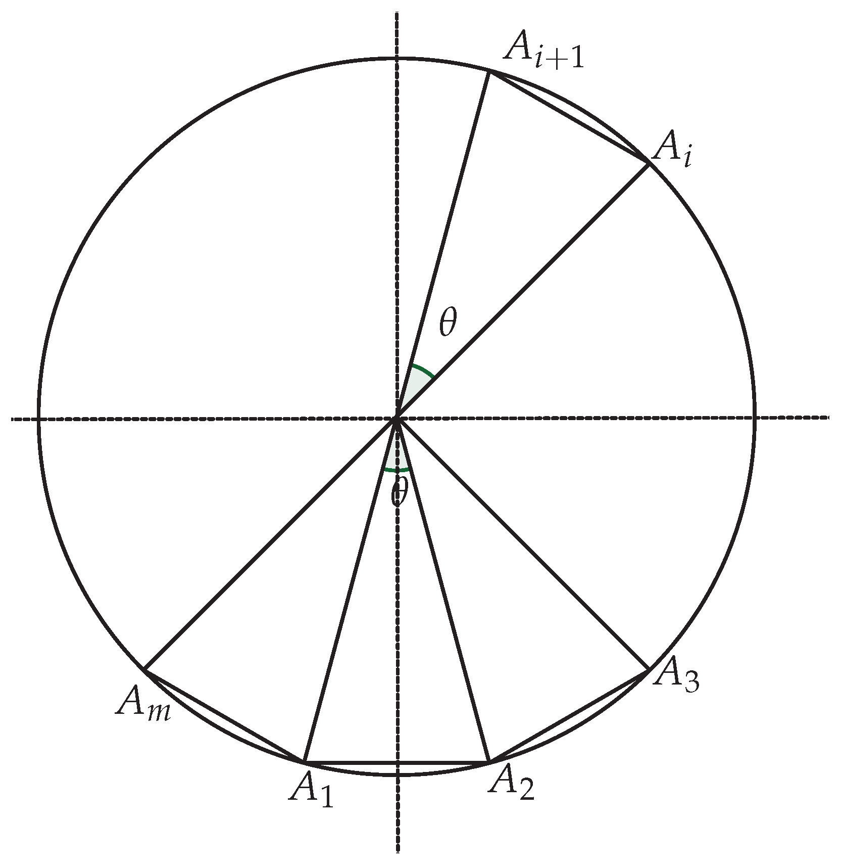
Hence, using the expressions in (12), we obtain

$$\begin{array}{cc}\hfill {\alpha }_n& =\left\{{\displaystyle \frac{1}{35}},{\displaystyle \frac{3}{35}},{\displaystyle \frac{1}{7}},{\displaystyle \frac{1}{5}},{\displaystyle \frac{1}{4}},{\displaystyle \frac{3}{10}},{\displaystyle \frac{7}{20}},{\displaystyle \frac{2}{5}},{\displaystyle \frac{7}{15}},{\displaystyle \frac{8}{15}},{\displaystyle \frac{3}{5}},{\displaystyle \frac{13}{20}},{\displaystyle \frac{7}{10}},{\displaystyle \frac{3}{4}},{\displaystyle \frac{4}{5}},{\displaystyle \frac{17}{20}},{\displaystyle \frac{9}{10}},{\displaystyle \frac{19}{20}},1\right\}with\hfill \\ \hfill V_n& =\sum _{j=1}^{5}V(P;\{{\alpha }_n\cap J_{k,j},J_{k,j}\})={\displaystyle \frac{2683}{10584000}}.\hfill \end{array}$$

5. Conditional Quantization for Uniform Distributions on the Boundaries of Regular Polygons Inscribed in a Unit Circle

Let the equation of the unit circle be $x_1^2+x_2^2=1$. Let $A_1{A}_2\cdots A_m$ be a regular m-sided polygon for some $m\ge 3$ inscribed in the circle, as shown in Figure 1. Let ℓ be the length of each side. Then, the length of the boundary of the polygon is given by $\ell m$. Let P be the uniform distribution defined on the boundary of the polygon. Then, the probability density function (pdf) f for the uniform distribution P is given by $f(x_1,x_2)={\displaystyle \frac{1}{m\ell }}$ for all $(x_1,x_2)\in A_1{A}_2\cdots A_m$, and zero otherwise. Let $\theta$ be the central angle subtended by each side of the polygon. Then, we know $\theta ={\displaystyle \frac{2\pi }{m}}$. Let the polar angles of the vertices $A_j$ of the polygon be given by ${\theta }_j$, where $1\le j\le m$. Without any loss of generality, due to rotational symmetry, we can always assume that the side $A_1{A}_2$ of the polygon is parallel to the $x_1$-axis, as shown in Figure 1. Then, we have

$${\theta }_1={\displaystyle \frac{3\pi }{2}}-{\displaystyle \frac{\theta }{2}}={\displaystyle \frac{3\pi }{2}}-{\displaystyle \frac{\pi }{m}}\mathrm{and}{\theta }_j={\theta }_1+(j-1){\displaystyle \frac{2\pi }{m}}\mathrm{for}2\le j\le m.$$

Let $\beta$ be the set of all vertices of the polygon, i.e.,

$$\beta :=\{(cos{\theta }_j,sin{\theta }_j):1\le j\le m\}.$$

Notice that the Cartesian coordinates of the vertices $A_1$ and $A_2$ are given by, respectively, $(-sin{\displaystyle \frac{\pi }{m}},-cos{\displaystyle \frac{\pi }{m}})$ and $(sin{\displaystyle \frac{\pi }{m}},-cos{\displaystyle \frac{\pi }{m}})$. Hence,

$$A_1{A}_2=\{(t,-cos{\displaystyle \frac{\pi }{m}}):-sin{\displaystyle \frac{\pi }{m}}\le t\le sin{\displaystyle \frac{\pi }{m}}\}.$$

Moreover, the length ℓ of each side is given by $\ell =2sin{\displaystyle \frac{\pi }{m}}.$ Let ${\alpha }_n$ be a conditional optimal set of n points for P with respect to the conditional set $\beta$, i.e., ${\alpha }_n$ exists for all $n\ge m$. Let

$$\mathrm{card}({\alpha }_n\cap A_i{A}_{i+1})=n_i\mathrm{where}1\le i\le m\mathrm{and}{A}_{m+1}\mathrm{is}\mathrm{identified}\mathrm{as}{A}_1.$$

(13)

Then, notice that

$$n_i\ge 2\mathrm{for}\mathrm{all}1\le i\le m\mathrm{and}{n}_1+n_2+\cdots +n_m=n+m,$$

as each of the vertices are counted two times.

Figure 1. The regular m-sided polygon inscribed in a unit circle.

Proposition 8. 

Let P be the uniform distribution defined on the boundary of the regular m-sided polygon inscribed in the unit circle. Let $card({\alpha }_n\cap A_1{A}_2)=n_1$. Then,

$$\begin{array}{cc}\hfill {\alpha }_n\cap A_1{A}_2& =\left\{\left(-sin{\displaystyle \frac{\pi }{m}}+{\displaystyle \frac{2(j-1)sin\frac{\pi }{m}}{n_1-1}},-cos{\displaystyle \frac{\pi }{m}}\right):1\le j\le n_1\right\}\hfill \end{array}$$

(14)

with the corresponding distortion error

$$V(P;\{{\alpha }_n\cap A_1{A}_2,A_1{A}_2\})={\displaystyle \frac{{sin}^2\frac{\pi }{m}}{3m{(n_1-1)}^2}}.$$

(15)

Proof. 

Notice that the line segment $A_1{A}_2$ is parallel to the $x_1$-axis and lies on the line $x_2=-cos{\displaystyle \frac{\pi }{m}}$. Hence, replacing c by $(-sin{\displaystyle \frac{\pi }{m}},-cos{\displaystyle \frac{\pi }{m}})$ and d by $(sin{\displaystyle \frac{\pi }{m}},-cos{\displaystyle \frac{\pi }{m}})$, by Proposition 1, we obtain

$${\alpha }_n\cap A_1{A}_2=\left\{\left(c_j,-cos{\displaystyle \frac{\pi }{m}}\right):1\le j\le n_1\right\},\mathrm{where}{c}_j=-sin{\displaystyle \frac{\pi }{m}}+{\displaystyle \frac{2(j-1)sin\frac{\pi }{m}}{m}}.$$

Recall $\ell =2sin{\displaystyle \frac{\pi }{m}}$. Hence,

$$\begin{array}{cc}\hfill V(P;\{{\alpha }_n\cap A_1{A}_2,A_1{A}_2\})& ={\displaystyle \frac{1}{m\ell }}(2{\int }_{c_1}^{{\displaystyle \frac{1}{2}}(c_1+c_2)}\rho ((t,-cos{\displaystyle \frac{\pi }{m}}),(c_1,-cos{\displaystyle \frac{\pi }{m}}))dt\hfill \\ \hfill & +(n_1-2){\int }_{{\displaystyle \frac{1}{2}}(c_1+c_2)}^{{\displaystyle \frac{1}{2}}(c_2+c_3)}\rho ((t,-cos{\displaystyle \frac{\pi }{m}}),(c_2,-cos{\displaystyle \frac{\pi }{m}}))dt)\hfill \\ \hfill & ={\displaystyle \frac{{sin}^2\frac{\pi }{m}}{3m{(n_1-1)}^2}},\hfill \end{array}$$

which yields the proposition.    □

The following lemma, which is similar to Lemma 2, is also true here.

Lemma 4. 

Let $n\in \mathbb{N}$ be such $n\ge m$. Let $n_i$ be the positive integers as defined by (13). Then, for $1\le i\ne j\le m$, $|n_i-n_j|=0or1$.

Let $T:{\mathbb{R}}^2\to {\mathbb{R}}^2$ be an affine transformations such that, for all $(x,y)\in {\mathbb{R}}^2$, we have

$$T(x,y)=(ax+by,cx+dy),$$

where

$$\begin{array}{cc}\hfill a& ={\displaystyle \frac{1}{2}}\left(sin{\displaystyle \frac{3\pi }{m}}csc{\displaystyle \frac{\pi }{m}}-1\right),b={\displaystyle \frac{1}{2}}\left(-sin{\displaystyle \frac{3\pi }{m}}sec{\displaystyle \frac{\pi }{m}}-tan{\displaystyle \frac{\pi }{m}}\right),\hfill \\ \hfill c& ={\displaystyle \frac{1}{2}}\left(cot{\displaystyle \frac{\pi }{m}}-cos{\displaystyle \frac{3\pi }{m}}csc{\displaystyle \frac{\pi }{m}}\right),\mathrm{and}d={\displaystyle \frac{1}{2}}\left(cos{\displaystyle \frac{3\pi }{m}}sec{\displaystyle \frac{\pi }{m}}+1\right).\hfill \end{array}$$

Also, for any $j\in \mathbb{N}$, by $T^j$ it is meant the composition mapping $T^j=T\circ T\circ T\circ \cdots j\mathrm{times}.$ If $j=0$, i.e., by $T^0$ it is meant the identity mapping on ${\mathbb{R}}^2$. Then, notice that

$$\begin{array}{cc}\hfill T^{i-1}(A_1{A}_2)& =A_i{A}_{i+1}\mathrm{for}1\le i\le m,\mathrm{where}{A}_{m+1}\mathrm{is}\mathrm{identified}\mathrm{as}{A}_1.\hfill \end{array}$$

Let us now give the following theorem, which is the main theorem is this section. This theorem helps us to determine the conditional optimal sets of n points and the nth conditional quantization errors for all $n\in \mathbb{N}$ with $n\ge m$.

Theorem 5. 

For $n\ge m$, let ${\alpha }_n$ be a conditional optimal set of n points such that $n=mk+\ell$ for some $k,\ell \in \mathbb{N}$ and $0\le \ell <m$. Then, identifying $A_{m+1}$ by $A_1$, we have

(i) 

if $\ell =0$, then $card({\alpha }_n\cap A_i{A}_{i+1})=k+1for1\le i\le m$;

(ii) 

if $1\le \ell <m$, then $card({\alpha }_n\cap A_i{A}_{i+1})=k+2fori\in \{i_1,i_2,\cdots ,i_{\ell }\}$ and $card({\alpha }_n\cap A_i{A}_{i+1})=k+1$ for $i\in \{1,2,\cdots ,m\}\setminus \{i_1,i_2,\cdots ,i_{\ell }\}$, where $\{i_1,i_2,\cdots ,i_{\ell }\}$ is any subset of ℓ elements of the set $\{1,2,\cdots ,m\}$.

Proof. 

The proof follows as a consequence of Lemma 4.    □

Conditional Optimal Sets of n Points and the nth Conditional Quantization Errors

Let $n\ge m$ be a positive integer. To determine the conditional optimal sets of n points and the nth conditional quantization errors, first using Theorem 5, we determine the values of $n_i$, where $n_i=\mathrm{card}({\alpha }_n\cap A_i{A}_{i+1})$ and $A_{m+1}$ is identified as $A_1$. Recall Proposition 8. For each $n_i$, assume that $\mathrm{card}({\alpha }_n\cap A_1{A}_2)=n_i$, and calculate ${\alpha }_n\cap A_1{A}_2$ and $V(P;\{{\alpha }_n\cap A_1{A}_2,A_1{A}_2\})$; denote them by ${\alpha }_n\cap A_1{A}_2(n_i)$ and $V(P;\{{\alpha }_n\cap A_1{A}_2,A_1{A}_2\})(n_i)$, respectively. Now, recall the affine transformation. Since the affine transformation considered in this section preserves the length, the distortion errors do not change under the affine transformation. Hence, for each $n_i$, we obtain ${\alpha }_n\cap A_i{A}_{i+1}$ and $V(P;\{{\alpha }_n\cap A_i{A}_{i+1},A_i{A}_{i+1}\})$ as follows:

$$\begin{array}{cc}& {\alpha }_n\cap A_i{A}_{i+1}=T^{i-1}\left({\alpha }_n\cap A_1{A}_2(n_i)\right),\mathrm{and}\hfill \\ \hfill V(P;\{{\alpha }_n& \cap A_i{A}_{i+1},A_i{A}_{i+1}\})=V(P;\{{\alpha }_n\cap A_1{A}_2,A_1{A}_2\})(n_i).\hfill \end{array}$$

Once ${\alpha }_n\cap A_i{A}_{i+1}$ and $V(P;\{{\alpha }_n\cap A_i{A}_{i+1},A_i{A}_{i+1}\})$ are obtained, we calculate the conditional optimal sets ${\alpha }_n$ and the nth conditional quantization errors using the following formulae:

$$\begin{array}{cc}\hfill {\alpha }_n& =\bigcup _{i=1}^m{T}^{i-1}\left({\alpha }_n\cap A_1{A}_2(n_i)\right)\hfill \\ \hfill & =\bigcup _{i=1}^m{T}^{i-1}\left\{\left(-sin{\displaystyle \frac{\pi }{m}}+{\displaystyle \frac{2(j-1)sin\frac{\pi }{m}}{n_i-1}},-cos{\displaystyle \frac{\pi }{m}}\right):1\le j\le n_i\right\}\hfill \end{array}$$

and

$$V_n=\sum _{i=1}^{m}V(P;\{{\alpha }_n\cap A_1{A}_2,A_1{A}_2\})(n_i)=\sum _{i=1}^m{\displaystyle \frac{{sin}^2\frac{\pi }{m}}{3m{(n_i-1)}^2}}.$$

□

Remark 2. 

Since the conditional quantization dimension is same as the quantization dimension (see [21]), and it is well known that the quantization dimension of an absolutely continuous probability measure equals the Euclidean dimension of the underlying space, we can assume that the conditional quantization dimension of P is one, i.e., $D(P)=1$.

Let us now give the following proposition.

Proposition 9. 

Let ${\alpha }_n$ be an optimal set of n points for P such that $n=mk$, where $k\in \mathbb{N}$. Then,

$$V_n={\displaystyle \frac{1}{3k^2}}{sin}^2{\displaystyle \frac{\pi }{m}}.$$

Proof. 

Let $n=mk$ for some $k\in \mathbb{N}$. Let $n_i$ be the positive integers as defined by (13). Then, by Lemma 4, we can say that

$$n_1=n_2=\cdots =n_m=k+1.$$

Notice that each $n_i$ equals $k+1$. It happens because ${\alpha }_n$ contains m distinct elements from each side, but in each $n_i$, both the end points are counted. Hence, by (15), we have $V_n={\displaystyle \frac{1}{3k^2}}{sin}^2{\displaystyle \frac{\pi }{m}}$. Thus, the proof of the proposition is complete.    □

Theorem 6. 

Let P be the uniform distribution on the boundary of a regular m-sided polygon inscribed in a unit circle. Then, the conditional quantization coefficient for P exists as a finite positive number and equals ${\displaystyle \frac{1}{3}}{m}^2{sin}^2({\displaystyle \frac{\pi }{m}})$, i.e., $\underset{n\to \infty }{lim}{n}^2(V_n-V_{\infty })={\displaystyle \frac{1}{3}}{m}^2{sin}^2({\displaystyle \frac{\pi }{m}}).$

Proof. 

Let $n\in \mathbb{N}$ be such that $n\ge m$. Then, there exists a unique positive integer $\ell (n)\ge 2$ such that $m\ell (n)\le n<m(\ell (n)+1)$. Then,

$${(m\ell (n))}^2{V}_{m(\ell (n)+1)}<n^2{V}_n<{(m(\ell (n)+1))}^2{V}_{m\ell (n)}.$$

(16)

Recall Proposition 9. By the squeeze theorem, we have $V_{\infty }={lim}_{n\to \infty }{V}_n=0.$ Moreover, we have

$$\begin{array}{cc}\hfill & \underset{n\to \infty }{lim}{(m\ell (n))}^2(V_{m(\ell (n)+1)}-V_{\infty })=\underset{n\to \infty }{lim}{(m\ell (n))}^2{\displaystyle \frac{1}{3{(\ell (n)+1)}^2}}{sin}^2{\displaystyle \frac{\pi }{m}}={\displaystyle \frac{1}{3}}{m}^2{sin}^2{\displaystyle \frac{\pi }{m}},\hfill \end{array}$$

and

$$\begin{array}{cc}\hfill & \underset{n\to \infty }{lim}{(m(\ell (n)+1))}^2(V_{m\ell (n)}-V_{\infty })=\underset{n\to \infty }{lim}{(m(\ell (n)+1))}^2{\displaystyle \frac{1}{3{(\ell (n))}^2}}{sin}^2{\displaystyle \frac{\pi }{m}}={\displaystyle \frac{1}{3}}{m}^2{sin}^2{\displaystyle \frac{\pi }{m}},\hfill \end{array}$$

and hence, by (16), using the squeeze theorem, we have $\underset{n\to \infty }{lim}{n}^2(V_n-V_{\infty })={\displaystyle \frac{1}{3}}{m}^2{sin}^2{\displaystyle \frac{\pi }{m}}$, i.e., the conditional quantization coefficient exists as a finite positive number that equals ${\displaystyle \frac{1}{3}}{m}^2{sin}^2{\displaystyle \frac{\pi }{m}}$. Thus, the proof of the theorem is complete.    □

Remark 3. 

It is known that for an absolutely continuous probability measure, the quantization dimension equals the Euclidean dimension of the underlying space, and the quantization coefficient exists as a finite positive number (see [24]). Since the conditional quantization dimension is the same as the quantization dimension, and the conditional quantization coefficient is the same as the quantization coefficient (see [21]), by Theorem 6, we can conclude that the quantization coefficient for the uniform distribution defined on the boundary of a regular m-sided polygon inscribed in a unit circle is ${\displaystyle \frac{1}{3}}{m}^2{sin}^2{\displaystyle \frac{\pi }{m}}$, which depends on m and is an increasing function of m. Thus, we can conclude that for absolutely continuous probability measures given in an Euclidean space, the quantization dimensions remain constant and is equal to the dimension of the underlying space, but the quantization coefficients can be different.

Let us now conclude the paper with the following remark.

Remark 4. 

Although the conditional quantization in this paper is investigated for uniform distributions on line segments and regular polygons, by using a similar technique or by giving a major overhaul of the technique given in this paper, interested researchers can explore them for any probability distribution defined on the boundary of any geometrical shape.