Limit Theorems for Kernel Regression Estimator for Quasi-Associated Functional Censored Time Series Within Single Index Structure

Abstract

In this paper, we develop kernel-based estimators for regression functions under a functional single-index model, applied to censored time series data. By capitalizing on the single-index structure, we reduce the dimensionality of the covariate-response relationship, thereby preserving the ability to capture intricate dependencies while maintaining a relatively parsimonious form. Specifically, our framework utilizes nonparametric kernel estimation within a quasi-association setting to characterize the underlying relationships. Under mild regularity conditions, we demonstrate that these estimators attain both strong uniform consistency and asymptotic normality. Through extensive simulation experiments, we confirm their robust finite-sample performance. Moreover, an empirical examination using intraday Nikkei stock index returns illustrates that the proposed method significantly outperforms traditional nonparametric regression approaches.

1. Introduction

The statistical analysis of single-index models has been thoroughly developed and examined from both theoretical and practical perspectives. Initial studies concentrated on models with vector explanatory variables, as emphasized by [1,2]. A significant advancement to the functional framework was introduced by [3], where explanatory variables are presented in an infinite-dimensional space, such as a Hilbert space. This advancement, known as the single functional index model, has attracted considerable attention due to its capacity to address two pivotal challenges: dimensionality reduction and interpretability. Specifically, the model alleviates the curse of dimensionality and offers meaningful insights through the interpretable index parameter, $\theta$.

The model investigated in this study lies between traditional single-index models and functional regression models, functioning as a generalization of the functional linear model. For instance, ref. [4] introduced a nonparametric estimation method for the link function using adaptive linear projections, demonstrating polynomial convergence rates. Building on this work, ref. [5] further extended functional linear regression models by proposing functional partially linear single-index models, utilizing least squares estimation to achieve similar convergence rates.

The single functional index model integrates the benefits of single-index models with the application potential of functional linear models [6] and nonparametric functional regression models [7,8,9,10,11,12,13,14]. Functional data modeling has become increasingly prominent, driven by technological advancements that allow for precise measurements and the generation of extensive datasets over continuous domains. However, most theoretical progress assumes independence among observations, a condition seldom met in practice. Instead, functional time series often display dependence, highlighting the necessity to explore models that relax the independence assumption.

This paper tackles the nonparametric estimation problem for regression functions in single functional index models under conditions of weak dependence. While strong mixing conditions are typically used to model dependence, this study adopts the more general quasi-association framework, initially introduced for real-valued random fields by [15]. Quasi-association extends the concept of positive association, as defined by [16], and can be considered a specific instance within the weak dependence framework outlined by [17].

From a practical perspective, quasi-associated data are crucial in areas such as reliability theory, mathematical physics, and percolation theory [18]. Theoretically, this correlation concept provides a unified approach to addressing both mixing and association dependencies in stochastic processes.

The single-index model, as a semi-parametric framework, bridges the strengths of parametric and nonparametric regression. Its application in multivariate statistics has been well documented by [2,19,20], with further developments made by [21,22,23]. In the realm of functional statistics, single functional index models have mainly been investigated for functional data, beginning with the foundational work of [3] on independent and identically distributed (i.i.d.) cases. Extensions to dependent data have been explored by [24,25]. Additionally, ref. [26] proposed a cross-validation-based estimation method for both nonparametric regression functions and linear coefficients, demonstrating its asymptotic optimality.

Subsequent research has introduced innovative estimation techniques. For example, ref. [27] utilized Bayesian methods to estimate bandwidths in kernel density and regression functions under autoregressive structures, showing enhanced predictive performance. ref. [28] developed a location-adaptive k-nearest neighbors approach for functional single-index models. Furthermore, ref. [29] created functional varying-coefficient single-index models for analyzing imaging data, while ref. [30] investigated Hilbertian regressors for the nonparametric estimation of conditional cumulative distributions. ref. [31] integrated multivariate random variables and random curves within a functional partial linear single-index framework. For recent works, refer to [32,33].

The concept of quasi-association for Hilbert space-valued random variables was introduced by [34], followed by limit theorems and regression-related advances, such as conditional density estimation [35] and asymptotic normality under dependence [36]. Other developments include local quadratic approximations for second-derivative link functions [37] and asymptotic normality for quasi-associated data in Hilbert spaces [38].

In this paper, we establish the almost complete convergence rates and asymptotic normality for the kernel single-index estimator in the context of censored data. This investigation represents a fundamentally unresolved open problem in the literature. Our objective is to bridge this gap by integrating the results of [34,39,40] with techniques designed to handle associated functional data and censored data. However, as will be demonstrated, the problem requires more than merely combining existing ideas. Instead, it requires intricate mathematical derivations to manage the associated functional data within our specific context, necessitating the effective application of large-sample theory techniques. Additionally, we establish the asymptotic distribution along with the corresponding confidence interval. This paper also includes a comprehensive section on the computational aspects of the proposed method, applied to both simulated and real data.

The remainder of this work is organized as follows. In Section 2, we describe the nonparametric model and the kernel estimator. Section 3 presents our primary results on the almost complete convergence of the Nadaraya–Watson kernel estimator under fairly general conditions. Section 4 discusses the asymptotic distribution. Section 5 provides the simulation results to illustrate the performance of the proposed method. In Section 6, we present a real data example. We conclude this paper with some remarks and suggestions for future work in Section 7. To maintain the flow of the presentation, all mathematical developments are deferred to Section 8.

2. Model and Estimator

2.1. Quasi-Associated Dependence

Stochastic models often involve families of random variables characterized by positive or negative dependence properties, or their variations. Foundational studies on this topic include [16,41,42,43]. To illustrate the concept, consider two finite samples separated by a gap r, with indices in the past denoted by $\left\{\mathrm{Pa}\right\}$, and in the future by $\left\{\mathrm{Fu}\right\}$. For certain classes of measurable functions, the independence of $\left\{\mathrm{Pa}\right\}$ and $\left\{\mathrm{Fu}\right\}$ can be expressed as the covariance $\mathrm{cov}\left(f\right(\mathrm{Fu}),g(\mathrm{Pa}\left)\right)=0$. A weaker form of this condition involves controlling these covariances as r increases, with the rate of decay defining the degree of weak dependence. For practical applications, this condition is often restricted to Lipschitz functions, making it easier to verify across a wide range of models. To define the quasi-association dependence in a Hilbert space $\mathcal{H}$ we define, in a first, and according to [15], this dependence in the real-valued random fields is as follows. Define a function $F:{\mathbb{R}}^n\to \mathbb{R}$ where ${\mathbb{R}}^n$ is equipped with its ${\mathit{\ell }}^1$-norm (i.e., $\parallel (x_1,\dots ,x_n){\parallel }_1=|x_1|+\cdots +|x_n|$) and define the Lipschitz modulus of $F(·)$ as

$$\mathrm{Lip}\left(F\right)={\displaystyle \underset{\mathbf{x}\ne \mathbf{y}}{sup}}{\displaystyle \frac{|F(\mathbf{x})-F(\mathbf{y})|}{{\parallel \mathbf{x}-\mathbf{y}\parallel }_1}}.$$

A sequence ${\left(Z_n\right)}_{n\in \mathbb{N}}$ of random variables is said to be quasi-associated if for any disjoint subsets I and J of $\mathbb{N}$, and all bounded Lipschitz functions $F_1:{\mathbb{R}}^{|I|}\to \mathbb{R}$ and $F_2:{\mathbb{R}}^{|J|}\to \mathbb{R}$ satisfying, this covariance exists:

$$\left|\mathrm{Cov}(F_1(Z_i,i\in I),F_2(Z_j,j\in J))\right|\le \mathrm{Lip}\left(F_1\right)\mathrm{Lip}\left(F_2\right){\displaystyle \sum _{i\in I}}{\displaystyle \sum _{j\in J}}\left|\mathrm{Cov}(Z_i,Z_j)\right|,$$

(1)

where $|I|$ denotes the cardinality of a finite set I, and $\mathrm{Cov}(Z_i,Z_j)$ the covariance of the pair $(Z_i,Z_j)$, respectively. Equation (1) is satisfied for positively associated or negatively associated random variables (see [44]). For example, ref. [45] demonstrated that any Gaussian random sequence with a covariance function taking both positive and negative values is quasi-associated.

Covariance inequalities are pivotal in establishing moment inequalities and limit theorems for dependent random variables [15,46] (and references therein). Independent real-valued random variables are inherently associated [47] and negatively associated [43]. A Gaussian random field is positively associated if its covariance function is non-negative [48], and negatively associated if $\mathrm{Cov}(X_s,X_t)\le 0$ for all $s\ne t$ [43]. The computational simplicity of covariance functions, as highlighted by [49] and others, often makes them preferable to mixing coefficients, which can be challenging to estimate.

The interplay between association and mixing is non-trivial, with overlapping yet distinct characteristics [17]. For instance, in linear time series, sequences defined by $X_k={\sum }_{j=0}^{\infty }{a}_j{v}_{k-j}$, where ${\left(v_i\right)}_{i\in \mathbb{Z}}$ are i.i.d. centered random variables with variance ${\sigma }^2$, are associated if $a_j\ge 0$. However, under suitable conditions on $a_j$, ref. [50] established $\alpha$-mixing for such sequences. Notably, ref. [51] showed that when $\left(v_i\right)$ are i.i.d. Bernoulli variables with $a_j=\varsigma$ and $0<\varsigma <1/2$, the sequence is associated but not $\alpha$-mixing. ref.  [34] extended the definition to functional random variables. Let us denote by the symbols $⟨·,·⟩$, and $\parallel ·\parallel$ the inner product and the associated norm on a Hilbert space $\mathcal{H}$, respectively, and we associate with this space a complete orthonormal system ${\left(e_p\right)}_{p\ge 1}$ of $\mathcal{H}$. A sequence ${\left(Z_i\right)}_{i\in \mathbb{N}}$ of random variables taking values in a Hilbert space $\mathcal{H}$ is called quasi-associated relative to an orthonormal basis $\{e_p:p\ge 1\}$ of $\mathcal{H}$, if for any $p\ge 1$, ${\left(⟨Z_i,e_1⟩,\dots ,⟨Z_i,e_p⟩\right)}_{i\in \mathbb{N}}$ is a sequence of quasi-associated random vectors.

Remark 1. 

Association and mixing are two distinct yet interrelated categories of stochastic processes, as elaborated on in [17]. The exploration of their respective dependence structures has drawn considerable academic attention. A fundamental difference lies in their interpretation of relationships among random variables: within the framework of association, independence can be inferred from the absence of correlation. This property, however, holds exclusively in the Gaussian setting, as noted in [47]. Thus, in Gaussian contexts, the covariance structure provides a complete description of dependence. This makes association an attractive property to study, since covariance calculations are typically more straightforward than those involving mixing coefficients.

In contrast, a major drawback of mixing processes is the limited number of models for which mixing coefficients can be explicitly determined. For example, consider the results in [52]: Let $\epsilon =\{{\epsilon }_i,i\in \mathbb{Z}\}$ be a stationary sequence of independent random variables with $\mathbb{E}{\epsilon }_0=0$ and ${\sigma }_0^2=\mathbb{E}{\epsilon }_1^2<\infty$. Let $a={\left\{a_n\right\}}_{n\in \mathbb{Z}}$ be a sequence of real numbers such that

$${\displaystyle \sum _{r\in \mathbb{Z}}}{a}_r^2<\infty .$$

Define the linear process $\{X_k,k\in \mathbb{Z}\}$ as

$$X_k:=\sum _{j=-\infty }^{\infty }{a}_j{\epsilon }_{k-j}.$$

This process is well-defined, strictly stationary, and satisfies $\mathbb{E}{X}_1^2<\infty$. This is denoted by ${\tilde{\mathcal{L}}}_2(a,\epsilon )$, the class of such linear sequences, and by ${\mathcal{L}}_2(a,\epsilon )$, the subset of ${\tilde{\mathcal{L}}}_2(a,\epsilon )$, where $a_i=0$ for $i<0$. If ${\epsilon }_0$ has an absolutely continuous density in ${\mathbb{L}}^1$, then any linear process $\{X_k,k\in \mathbb{Z}\}$ within ${\mathcal{L}}_2(a,\epsilon )$ is absolutely regular (β-mixing) with coefficients satisfying the following:

$${\beta }_n\le K{\displaystyle \sum _{j\ge n}}{\left({\displaystyle \sum _{k\ge j}}|a_k|\right)}^{2/3},\mathit{for}\mathit{some}\mathit{constant}K,$$

provided that

$${\displaystyle \sum _{j\ge 0}}{\left({\displaystyle \sum _{k\ge j}}|a_k|\right)}^{2/3}<\infty ,$$

as established in [50].

1. 

Associated but not mixing sequences: Consider the sequence $\epsilon =\{{\epsilon }_i,i\in \mathbb{Z}\}$, where ${\epsilon }_i$ are i.i.d. random variables with $\mathbb{P}({\epsilon }_i=1)=\mathbb{P}({\epsilon }_i=0)=1/2$. Let $a=\{2^{-k},k\ge 1\}$. The linear process $\left\{X_k\right\}\in {\mathcal{L}}_2(a,\epsilon )$ is associated (see $\left({\mathcal{P}}_2\right)$ and $\left({\mathcal{P}}_4\right)$ in [16]) but not mixing, as ${\beta }_n\ge 1/4$ (refer to [53]). Furthermore, $X_1$ follows a uniform distribution on $[0,1]$, and its covariance function satisfies

$$r\left(n\right):=Cov(X_1,X_n)=c^2{\sigma }_0^2{2}^{-n},$$

exhibiting exponential decay. The associated empirical process $\{G_n\left(x\right):x\in \mathbb{R}\}$ converges, as demonstrated in [54].

2. 

Associated and mixing sequences: When the conditions of Theorem 2.1 in [50] hold, and $a_k\ge 0$ for all $k\in \mathbb{N}$, the linear process $\left\{X_k\right\}\in {\mathcal{L}}_2(a,\epsilon )$ exhibits both association and β-mixing properties.

3. 

Mixing but not associated sequences: Consider a sequence $a=\{a_k,k\in \mathbb{N}\}$ satisfying $a_0{a}_1<0$ and $a_i=0$ for $i\ge 2$. Then, $X_n=a_0{\epsilon }_n+a_1{\epsilon }_{n-1}$ is not associated, as 

$$Cov(X_n,X_{n-1})=a_0{a}_1{\sigma }_0^2<0,$$

violating the association condition. However, the sequence $\left\{X_n\right\}$ is mixing due to its m-dependence.

2.2. The Single Functional Index Model

Let $\{(X_i,C_i,Y_i^0),1\le i\le n\}$ be n copies i.i.d. of a triplet of random variables $(X,C,Y^0)$, where X takes values in a separable real Hilbert space $\mathcal{H}$ endowed with the inner product $⟨·,·⟩$ and its norm $\parallel ·\parallel ={⟨·,·⟩}^{1/2}$, and C is a censoring variable with real values and $Y^0$ is the variable of interest, typically called a lifetime variable. We consider the semi-metric $d_{\theta },$ associated with the single-index $\theta$, which is defined by $d_{\theta }({\chi }_1,{\chi }_2):=|⟨{\chi }_1-{\chi }_2,\theta ⟩|$. In the given topological structure, and for any $\theta$, our focus is to estimate nonparametrically the conditional mean (regression) function of $Y^0$ given $⟨X,\theta ⟩$, denoted by

$$r_{\theta }\left(\chi \right):=\mathrm{I}\mathrm{E}(Y^0|⟨\theta ,X⟩=⟨\theta ,\chi ⟩).$$

(2)

Since the single functional index $\theta$ plays a crucial role in such a model, the identifiability of this model will be important. Clearly, the relation in (2) can be reformulated as $Y^0=r\left(⟨X,\theta ⟩\right)+ϵ$ with $\mathrm{I}\mathrm{E}(ϵ|X)=0$. To ensure the identifiability of the model $\theta$ (i.e., ${\theta }_1={\theta }_2$), we require that $r_j\left(⟨\chi ,{\theta }_j⟩\right)$ is differentiable with respect to (wrt) the variable $⟨\chi ,{\theta }_j⟩,j=1,2$, respectively, and that $⟨\theta ,e_1⟩=1$, where $e_1$ is the first element of an orthonormal basis of the space $\mathcal{H}$. Then, for all $\chi \in \mathcal{H}$, $r_1\left(⟨\chi ,{\theta }_1⟩\right)=r_2\left(⟨\chi ,{\theta }_2⟩\right)$ implies $r_1=r_2$ and ${\theta }_1={\theta }_2$, respectively. For more details on the proof of the identifiability of the functional single model, see [3].

It is worth highlighting that when censored data are considered, the smoothing nonparametric regression estimator $\widehat{r}(\theta ,\chi )$ of $r(\theta ,\chi )$ can be viewed as a local least squares estimator that is

$$\begin{array}{ccc}\hfill \widehat{r}(\theta ,\chi )& =& {\displaystyle arg{\displaystyle \underset{t\in \mathrm{I}\mathrm{R}}{min}}\sum _{i=1}^n{W}_{i,n}(\theta ,\chi ){(Y_i-t)}^2.}\hfill \end{array}$$

where $W_{i,n}(\theta ,\chi )$ are the Nadaraya–Watson weights [55,56], given as

$$\begin{array}{ccc}\hfill W_{i,n}(\theta ,\chi )& =& {\displaystyle \frac{K(h_n^{-1}|⟨\chi -X_i,\theta ⟩|)}{{\displaystyle \sum _{i=1}^{n}K(h_n^{-1}|⟨\chi -X_i,\theta ⟩|)}}.}\hfill \end{array}$$

A natural estimator of $r(\theta ,\chi )$ is defined as

$$\begin{array}{c}\hfill {\displaystyle \widehat{r}(\theta ,\chi )=\sum _{i=1}^n{Y}_i^0{W}_{i,n}(\theta ,\chi )=\frac{{\displaystyle \sum _{i=1}^n{Y}_i^{0}K(h_n^{-1}|⟨\chi -X_i,\theta ⟩|)}}{{\displaystyle \sum _{i=1}^{n}K(h_n^{-1}|⟨\chi -X_i,\theta ⟩|)}}.}\end{array}$$

(3)

where $K(·)$ is a kernel function, and $h_n:=h_{n,K}$ is a sequence of bandwidths (positive real numbers) decreasing to zero as n goes to infinity.

As is known, when dealing with censoring data, the first problem arising is understanding and managing the censorship itself, due to incomplete or partial collected observations. One of the suggested approaches to tackling censored data is to apply the method of synthetic data, which allows us to take into account the censoring effect on the lifetime distribution, for instance, [57,58,59]. Theoretically, synthetic data transformation provides equal expected values for both variables. In this case, the synthetic response variable (transformed variable) is given by ${\displaystyle \frac{{\delta }_i{Y}_i}{\overline{G}\left(Y_i\right)},1\le i\le n}$, where $\overline{G}=1-G$, and if we assume $(Y_i^0,X_i)$ and $\left(C_i\right)$ are independent (that is usually supposed for censored data), we obtain

$$\begin{array}{ccc}\hfill \mathrm{I}\mathrm{E}\left[{\displaystyle \frac{{\delta }_i{Y}_i}{\overline{G}\left(Y_i\right)}}|X_i\right]& =& \mathrm{I}\mathrm{E}\left\{\mathrm{I}\mathrm{E}\left[{\displaystyle \frac{{\delta }_i{Y}_i}{\overline{G}\left(Y_i\right)}}|Y_i^0,X_i\right]|X_i\right\}\hfill \\ & =& \mathrm{I}\mathrm{E}\left\{\mathrm{I}\mathrm{E}\left[{\displaystyle \frac{{\mathbb{1}}_{\{Y_i^0\le C_i\}}{Y}_i}{\overline{G}\left(Y_i\right)}}|Y_i^0,X_i\right]|X_i\right\}\hfill \\ & =& \mathrm{I}\mathrm{E}\left\{{\displaystyle \frac{Y_i^0}{\overline{G}\left(Y_i^0\right)}}\mathrm{I}\mathrm{E}\left[{\mathbb{1}}_{\{Y_i^0\le C_i\}}|Y_i^0\right]|X_i\right\}\hfill \\ & =& \mathrm{I}\mathrm{E}\left[Y_i^0|X_i\right].\hfill \end{array}$$

(4)

By the same manner, we get by conditioning wrt $⟨\theta ,X_i⟩$

$$\begin{array}{ccc}\hfill \mathrm{I}\mathrm{E}\left[{\displaystyle \frac{{\delta }_i{Y}_i}{\overline{G}\left(Y_i\right)}}|⟨\theta ,X_i⟩\right]& =& \mathrm{I}\mathrm{E}\left[Y_i^0|⟨\theta ,X_i⟩\right].\hfill \end{array}$$

(5)

Thus, for the infinite dimension case, one can define the pseudo-estimator of $r_{\theta }\left(\chi \right)$ as

$$\begin{array}{c}\hfill {\displaystyle \tilde{r}(\theta ,\chi )=\frac{{\displaystyle \sum _{i=1}^n\frac{{\delta }_i{Y}_i}{\overline{G}\left(Y_i\right)}K(h_n^{-1}|⟨\chi -X_i,\theta ⟩|)}}{{\displaystyle \sum _{i=1}^{n}K(h_n^{-1}|⟨\chi -X_i,\theta ⟩|)}}=\frac{{\tilde{r}}_N(\theta ,\chi )}{{\widehat{r}}_D(\theta ,\chi )}.}\end{array}$$

(6)

where

$$\begin{array}{ccc}\hfill {\tilde{r}}_N(\theta ,\chi )& =& {\displaystyle \frac{1}{n\mathrm{I}\mathrm{E}\left[K_1(\theta ,\chi )\right]}}\sum _{i=1}^n{\displaystyle \frac{{\delta }_i{Y}_i}{\overline{G}\left(Y_i\right)}}{K}_i(\theta ,\chi )\hfill \\ \hfill {\widehat{r}}_D(\theta ,\chi )& =& {\displaystyle \frac{1}{n\mathrm{I}\mathrm{E}\left[K_1(\theta ,\chi )\right]}}\sum _{i=1}^n{K}_i(\theta ,\chi )\hfill \\ \hfill K_i(\theta ,\chi )& =& K(h_n^{-1}|⟨\chi -X_i,\theta ⟩|)=K\left(h_n^{-1}{d}_{\theta }(\chi ,X_i)\right).\hfill \end{array}$$

In practice, since the values $Y^0$ are censored observations, the survival function $\overline{G}(·)=1-G(·)$ is unknown (because $G(·)$ is too), so it is impossible to use the estimator (6). To complete building a good estimator of $r(\theta ,\chi )$, we may replace the function $\overline{G}(·)$ by its corresponding [60] estimator ${\overline{G}}_n(·):=1-G_n(·)$, defined by

$$\begin{array}{c}\hfill {\overline{G}}_n\left(t\right)=\left\{\begin{array}{cc}{\displaystyle \prod _{i=1}^n{\left({\displaystyle 1-\frac{1-{\delta }_{\left(i\right)}}{n-i+1}}\right)}^{{\mathbb{1}}_{\{Y_{\left(i\right)}\le t\}}},}\hfill & \mathrm{if}t<Y_{\left(n\right)},\hfill \\ 0,\hfill & \mathrm{if}t\ge Y_{\left(n\right)}.\hfill \end{array}\right.\end{array}$$

(7)

where $Y_{\left(1\right)}\le Y_{\left(2\right)}\le \cdots \le Y_{\left(n\right)}$ are the order statistics of $Y_i$ and ${\delta }_{\left(i\right)}$ is the indicator of no censoring associated with $Y_{\left(i\right)}$. We will set ${log}_{2}u={log}_{+}\left({log}_{+}u\right),{log}_{+}u=log(u\vee e)$. ref. [61] obtained the law of iterated logarithms for the censored case. More precisely, for a continuous G, we have as $n\to \infty ;$

$${\displaystyle {\displaystyle \underset{0\le t\le Y_{\left(n\right)}}{sup}}\left|\frac{1}{G_n\left(t\right)}-\frac{1}{G\left(t\right)}\right|=O\left({\left(\frac{{log}_{2}n}{n}\right)}^{\frac{1}{2}}\right),}$$

almost surely. Such a result will be useful to establish the main results of this paper. Now, plugging the estimator (7) in (6), one can define an estimator of $r(\theta ,\chi )$ as

$$\begin{array}{c}\hfill {\widehat{r}}_n(\theta ,\chi )={\displaystyle \frac{{\displaystyle \frac{1}{n\mathrm{I}\mathrm{E}\left[K_1(\theta ,\chi )\right]}\sum _{i=1}^n\frac{{\delta }_i{Y}_i}{{\overline{G}}_n\left(Y_i\right)}K(h_n^{-1}|⟨\chi -X_i,\theta ⟩|)}}{{\displaystyle \frac{1}{n\mathrm{I}\mathrm{E}\left[K_1(\theta ,\chi )\right]}\sum _{i=1}^{n}K(h_n^{-1}|⟨\chi -X_i,\theta ⟩|)}}}=:{\displaystyle \frac{{\widehat{r}}_N(\theta ,\chi )}{{\widehat{r}}_D(\theta ,\chi )}}.\end{array}$$

(8)

The covariance coefficient ${\lambda }_r$ defined as

$${\displaystyle {\lambda }_r:={\displaystyle \underset{s\ge r}{sup}}{\displaystyle \sum _{|i-j|\ge s}}{\lambda }_{i,j},}$$

where

$$\begin{array}{ccc}\hfill {\lambda }_{i,j}& =& {\displaystyle {\displaystyle \sum _{k\ge 1}}{\displaystyle \sum _{l\ge 1}}\left|Cov(X_i^k,X_j^l)\right|+{\displaystyle \sum _{k\ge 1}}\left|Cov(X_i^k,Y_j)\right|}\hfill \\ & & {\displaystyle +{\displaystyle \sum _{l\ge 1}}\left|Cov(Y_i,X_j^l)\right|+\left|Cov(Y_i,Y_j)\right|,}\hfill \end{array}$$

with $X_i^p:=⟨X_i,e_p⟩$.

3. Strong Uniform Consistency

3.1. Results

Throughout this manuscript, provided that no ambiguity arises, we will denote by C, $C^{\prime }$, and/or $C_{\theta ,x}$ generic positive constants, which may vary with each occurrence. For any sequences $\left(u_n\right)$ and $\left(v_n\right)$, we write $u_n=O\left(v_n\right)$, provided that $|u_n|\le C|v_n|$ for all n. If this condition holds almost completely, we use the notation $O_{a.co.}$. Let ${\mathcal{N}}_{\chi }$ represent a fixed neighborhood of a point $\chi$ in the space $\mathcal{H}$, and define the ball centred at $\chi$ with radius r by

$${\mathcal{B}}_{\theta }(\chi ,r):=\{{\chi }_1\in \mathcal{H}\mid |⟨\chi -{\chi }_1,\theta ⟩|<r\}.$$

Define the upper endpoints of the distributions F and G by

$${\tau }_F=sup\{y\mid \overline{F}\left(y\right)>0\}\mathrm{and}{\tau }_G=sup\{y\mid \overline{G}\left(y\right)>0\}.$$

We assume that ${\tau }_F$ is finite and that $\overline{G}\left({\tau }_F\right)>0$, which implies that ${\tau }_F<{\tau }_G$.

Consider the following coverings of the compact sets $S_{\mathcal{H}}$ and ${\Theta }_{\mathcal{H}}$:

$$S_{\mathcal{H}}\subset \bigcup _{k=1}^{d_n^{S_{\mathcal{H}}}}B({\chi }_k,l_n)\mathrm{and}{\Theta }_{\mathcal{H}}\subset \bigcup _{j=1}^{d_n^{{\Theta }_{\mathcal{H}}}}B(t_j,l_n),$$

where ${\chi }_k,t_j\in \mathcal{H}$. For each $\chi \in \mathcal{H}$ and $\theta \in {\Theta }_{\mathcal{H}}$, define

$$k\left(\chi \right)=arg{\displaystyle \underset{k\in \{1,\dots ,d_n^{S_{\mathcal{H}}}\}}{min}}\parallel \chi -{\chi }_k\parallel \mathrm{and}j\left(\theta \right)=arg{\displaystyle \underset{j\in \{1,\dots ,d_n^{{\Theta }_{\mathcal{H}}}\}}{min}}\parallel \theta -t_j\parallel .$$

It is important to note that covering the compact subsets in this manner is essential for establishing our uniform consistency. Additionally, this approach is crucial to maintaining the geometric relationship between the numbers $d_n^{S_{\mathcal{H}}}$, $d_n^{{\Theta }_{\mathcal{H}}}$ of balls and the sequence of the radius $l_n$. In the context of abstract semi-metric spaces, it is generally assumed that $d_n^{S_{\mathcal{H}}}{l}_n$ and $d_n^{{\Theta }_{\mathcal{H}}}{l}_n$ remain bounded (see [26], for further discussion).

We now present the assumptions necessary to derive our initial result:

(A0)

The random variables $(X,Y^0)$ and C are independent.

(A1)

(i)

The probability $\mathrm{I}\mathrm{P}(X\in {\mathcal{B}}_{\theta }(\chi ,ϵ))$, denoted by ${\varphi }_{\theta ,\chi }\left(ϵ\right)$, is positive for all $ϵ>0$, and satisfies

$${\displaystyle \underset{ϵ\to 0}{lim}}{\varphi }_{\theta ,\chi }\left(ϵ\right)=0.$$

(ii)

There exists a differentiable function $\varphi (·)$ such that for all $\chi \in S_{\mathcal{H}}$ and $\theta \in {\Theta }_{\mathcal{H}}$,

$$0<C\varphi \left(h_n\right)\le {\varphi }_{\theta ,\chi }\left(h_n\right)\le C^{\prime }\varphi \left(h_n\right)<\infty ,$$

and there exists a constant ${\xi }_0>0$ for which

$${\varphi }^{\prime }\left(\xi \right)<C\mathrm{for}\mathrm{all}\xi <{\xi }_0.$$

(A2)

The function $r(·,·)$ satisfies a Hölder condition. Specifically, for all $\theta \in \mathcal{H}$ and for all $({\chi }_1,{\chi }_2)\in {\mathcal{N}}_{\chi }\times {\mathcal{N}}_{\chi }$,

$$|r(\theta ,{\chi }_1)-r(\theta ,{\chi }_2)|\le C_{\theta ,\chi }{d}_{\theta }{({\chi }_1,{\chi }_2)}^{\gamma },$$

where $\gamma >0$.

(A3)

The function $K(·)$ is bounded and continuous, and satisfies the following conditions:

(i)

There exist constants $C,C^{\prime }>0$ such that

$$0<C{\mathbb{1}}_{[0,1]}\left(t\right)<K\left(t\right)<C^{\prime }{\mathbb{1}}_{[0,1]}\left(t\right)<\infty \mathrm{for}\mathrm{all}t.$$

(ii)

For all $t_1,t_2\in \mathbb{R}$,

$$|K\left(t_1\right)-K\left(t_2\right)|\le C|t_1-t_2|.$$

(A4)

Let $l_n=O\left({\displaystyle \frac{logn}{n}}\right)$. The sequences $d_n^{S_{\mathcal{H}}}$ and $d_n^{{\Theta }_{\mathcal{H}}}$ satisfy

(i)

$${\displaystyle \frac{{(logn)}^2}{n\varphi \left(h_n\right)}}<log{d}_n^{S_{\mathcal{H}}}+log{d}_n^{{\Theta }_{\mathcal{H}}}<{\displaystyle \frac{n\varphi \left(h_n\right)}{logn}}.$$

(ii)

$$\sum _{n=1}^{\infty }{\left(d_n^{S_{\mathcal{H}}}{d}_n^{{\Theta }_{\mathcal{H}}}\right)}^{1-\beta }<\infty \mathrm{for}\mathrm{some}\beta >2.$$

(iii)

$$n\varphi \left(h_n\right)=O\left({(logn)}^2\right)\mathrm{and}{\displaystyle \underset{n\to \infty }{lim}}n\varphi \left(h_n\right)=\infty .$$

(A5)

The process ${(X_i,Y_i)}_{i\in \mathbb{N}}$ is quasi-associated with a covariance coefficient ${\lambda }_k$ that satisfies

$$\exists a>0,\exists C>0\mathrm{such}\mathrm{that}\forall k\in \mathbb{N},{\lambda }_k\le C{e}^{-ak}.$$

(A6)

$$0<{\displaystyle \underset{i\ne j}{sup}}\mathrm{I}\mathrm{P}\left((X_i,X_j)\in {\mathcal{B}}_{\theta }(\chi ,h_n)\times {\mathcal{B}}_{\theta }(\chi ,h_n)\right)=O\left({\varphi }_{\theta ,\chi }{\left(h_n\right)}^2\right).$$

(A7)

(i)

There exists a constant $0<\rho <{\displaystyle \frac{1}{2}}$ such that

$${\varphi }_{\theta ,\chi }\left(h_n\right)\ge h_n^{{\displaystyle \frac{2\rho }{1-2\rho }}}.$$

(ii)

$${\displaystyle \underset{n\to \infty }{lim}}{\displaystyle \frac{{log}^5\left(n\right)}{n{\varphi }_{\theta ,\chi }\left(h_n\right)}}=0.$$

Remark 2. 

Assumption (A0) typically serves as the independence condition necessary to ensure identifiability within the random censoring framework. In the absence of (A0), additional information regarding the structure of censoring must be provided. Furthermore, the condition ${\tau }_F<{\tau }_G$ (which implies $\overline{G}\left(Y^0\right)>\overline{G}\left({\tau }_F\right)$) is a standard assumption for establishing asymptotic results in censoring contexts. Assumption (A1) characterizes the concentration of the explanatory variable within small neighborhoods, and it is fundamentally important for deriving various asymptotic properties, especially when dealing with functional data. Assumption (A2) is necessary to control the bias term in convergence rates and to ensure the regularity of the model. Assumptions (A3) and (A4) are technical in nature and facilitate the evaluation of the asymptotic variance component. Assumption (A5) provides an upper bound for the polynomial decay of the association coefficient, while Assumption (A6) describes the asymptotic behavior of the joint distribution of the pair $(X_i,X_j)$. Finally, Assumption (A7) is included for the sake of brevity in the proofs, as it satisfies technical requirements, particularly when applying the exponential inequality introduced by [39].

The proof of Theorem 1 relies on the subsequent lemmas, whose proofs are provided in Section 8.

Lemma 1. 

Under assumptions (A0), (A1), (A3), and (A4), we have

$$\begin{array}{c}\hfill {\displaystyle \underset{\chi \in S_{\mathcal{H}}}{sup}}{\displaystyle \underset{\theta \in {\Theta }_{\mathcal{H}}}{sup}}\left|{\tilde{r}}_1(\theta ,\chi )-\mathbb{E}\left[{\tilde{r}}_1(\theta ,\chi )\right]\right|=O_{a.co.}\left(\sqrt{{\displaystyle \frac{log{d}_n^{S_{\mathcal{H}}}+log{d}_n^{{\Theta }_{\mathcal{H}}}}{n\varphi \left(h_n\right)}}}\right).\end{array}$$

Lemma 2. 

Under assumptions (A1) and (A3) through (A7), the following holds:

$$\begin{array}{c}\hfill {\displaystyle \underset{\chi \in S_{\mathcal{H}}}{sup}}{\displaystyle \underset{\theta \in {\Theta }_{\mathcal{H}}}{sup}}\left|{\widehat{r}}_2(\theta ,\chi )-1\right|=O_{a.co.}\left(\sqrt{{\displaystyle \frac{log{d}_n^{S_{\mathcal{H}}}+log{d}_n^{{\Theta }_{\mathcal{H}}}}{n\varphi \left(h_n\right)}}}\right).\end{array}$$

Corollary 1. 

From Lemma 2, it follows that

$$\begin{array}{c}\hfill \sum _{n=1}^{\infty }\mathbb{P}\left({\displaystyle \underset{\theta \in {\Theta }_{\mathcal{H}}}{inf}}{\displaystyle \underset{\chi \in \mathcal{H}}{inf}}\left|{\widehat{r}}_2(\theta ,\chi )\right|<{\displaystyle \frac{1}{2}}\right)<\infty .\end{array}$$

(9)

Lemma 3. 

Assuming (A0), (A1), (A3), and (A4), we have

$$\begin{array}{c}\hfill {\displaystyle \underset{\chi \in S_{\mathcal{H}}}{sup}}{\displaystyle \underset{\theta \in {\Theta }_{\mathcal{H}}}{sup}}\left|{\widehat{r}}_1(\theta ,\chi )-{\tilde{r}}_1(\theta ,\chi )\right|=O_{a.co.}\left(\sqrt{{\displaystyle \frac{log{d}_n^{S_{\mathcal{H}}}+log{d}_n^{{\Theta }_{\mathcal{H}}}}{n\varphi \left(h_n\right)}}}\right).\end{array}$$

Lemma 4. 

Under assumptions (A0), (A1)-(i), and (A2), it holds that

$$\begin{array}{c}\hfill {\displaystyle \underset{\chi \in S_{\mathcal{H}}}{sup}}{\displaystyle \underset{\theta \in {\Theta }_{\mathcal{H}}}{sup}}\left|\mathbb{E}\left[{\tilde{r}}_1(\theta ,\chi )\right]-r(\theta ,\chi )\right|=O\left(h_n^{\gamma }\right).\end{array}$$

We present the following main theorem on this section.

Theorem 1. 

Assume that conditions (A0) through (A7) are satisfied. Then, the following holds:

$$\begin{array}{ccc}\hfill {\displaystyle \underset{\chi \in S_{\mathcal{H}}}{sup}}{\displaystyle \underset{\theta \in {\Theta }_{\mathcal{H}}}{sup}}\left|{\widehat{r}}_n(\theta ,\chi )-r(\theta ,\chi )\right|& =& O\left(h_n^{\gamma }\right)+O_{a.co.}\left(\sqrt{{\displaystyle \frac{log{d}_n^{S_{\mathcal{H}}}+log{d}_n^{{\Theta }_{\mathcal{H}}}}{n\varphi \left(h_n\right)}}}\right).\hfill \end{array}$$

Proof of Theorem 1. 

We begin by considering the following decomposition:

$$\begin{array}{ccc}\hfill {\widehat{r}}_n(\theta ,\chi )-r(\theta ,\chi )& =& {\displaystyle \frac{{\widehat{r}}_1(\theta ,\chi )-r(\theta ,\chi ){\widehat{r}}_2(\theta ,\chi )}{{\widehat{r}}_2(\theta ,\chi )}}\hfill \\ & =& {\displaystyle \frac{{\widehat{r}}_1(\theta ,\chi )-{\tilde{r}}_1(\theta ,\chi )}{{\widehat{r}}_2(\theta ,\chi )}}+{\displaystyle \frac{{\tilde{r}}_1(\theta ,\chi )-\mathbb{E}\left[{\tilde{r}}_1(\theta ,\chi )\right]}{{\widehat{r}}_2(\theta ,\chi )}}\hfill \\ & & +{\displaystyle \frac{\mathbb{E}\left[{\tilde{r}}_1(\theta ,\chi )\right]-r(\theta ,\chi )}{{\widehat{r}}_2(\theta ,\chi )}}+r(\theta ,\chi ){\displaystyle \frac{1-{\widehat{r}}_2(\theta ,\chi )}{{\widehat{r}}_2(\theta ,\chi )}}.\hfill \end{array}$$

(10)

The result of the theorem is obtained by synthesizing the findings of the preceding lemmas.    □

In the specific case where the functional single index is held fixed, the following corollary applies.

Corollary 2. 

Under assumptions (A0) through (A7), it holds that

$$\begin{array}{ccc}\hfill {\displaystyle \underset{\chi \in S_{\mathcal{H}}}{sup}}\left|{\widehat{r}}_n(\theta ,\chi )-r(\theta ,\chi )\right|& =& O\left(h_n^{\gamma }\right)+O_{a.co.}\left(\sqrt{{\displaystyle \frac{log{d}_n^{S_{\mathcal{H}}}}{n\varphi \left(h_n\right)}}}\right).\hfill \end{array}$$

3.2. Methodology for Estimating a Single Functional Index

In practice, the functional index is unknown and must be estimated. Two main approaches are available for this purpose. The first is the Least Squares Cross-Validation (LSCV) method, defined by

$$\widehat{\theta }=arg{\displaystyle \underset{\theta \in \Theta }{min}}{\displaystyle \frac{1}{n}}\sum _{i=1}^n{\left(Y_i-{\widehat{r}}_n^{-i}(\theta ,X_i)\right)}^2,$$

(11)

where ${\widehat{r}}_n^{-i}(\theta ,\chi )$ denotes the leave-one-out estimator of ${\widehat{r}}_n(\theta ,\chi )$. The second is the Maximum Likelihood Cross-Validation (MLCV) method, given by

$$\widehat{\theta }=arg{\displaystyle \underset{\theta \in \Theta }{min}}{\displaystyle \frac{1}{n}}\sum _{i=1}^{n}log\widehat{f}\left(Y_i\mid {\widehat{r}}_n^{-i}(\theta ,X_i)\right),$$

(12)

where $\widehat{f}(·\mid ·)$ is the estimator of the conditional density of Y given $⟨\theta ,X⟩$. In practice, both of these methods require optimizing over a finite subset $\Theta$.

Following [26], we propose selecting the optimal index from the set

$$\Theta ={\Theta }_n=\left\{\theta \in H:\theta =\sum _{i=1}^k{c}_i{e}_i,\parallel \theta \parallel =1,\exists j\in \{1,\dots ,k\}\mathrm{such}\mathrm{that}⟨\theta ,e_j⟩>0\right\},$$

(13)

where ${\left\{e_i\right\}}_{i=1,\dots ,k}$ is a finite basis of the Hilbert subspace spanned by the covariates ${\left\{X_i\right\}}_i$, and ${\left\{c_i\right\}}_i$ are real-valued constants calibrated to ensure the identifiability of the model (commonly, $c_i\in \{-1,0,1\}$). It is well known that cross-validation methods can be used to estimate any parameter within this framework.

An alternative approach—which will be used in this section—is to choose $\theta \left(t\right)$ from the eigenfunctions of the covariance operator

$$\mathbb{E}\left[\left(X^{\prime }-\mathbb{E}\left[X^{\prime }\right]\right){⟨X^{\prime },·⟩}_{\mathcal{H}}\right],$$

where $X\left(t\right)$ is, for instance, a diffusion-type process defined by $[a,b]$, and $X^{\prime }\left(t\right)$ denotes its first derivative (see [30]). Given a training sample $\mathcal{L}$, the covariance operator can be estimated by its empirical version

$${\displaystyle \frac{1}{|\mathcal{L}|}}{\displaystyle \sum _{i\in \mathcal{L}}}{\left(X_i^{\prime }-\mathbb{E}\left[X^{\prime }\right]\right)}^t\left(X_i^{\prime }-\mathbb{E}\left[X^{\prime }\right]\right).$$

A discretized version of the eigenfunctions $\left\{{\theta }_i\left(t\right)\right\}$ can then be obtained using principal component analysis, as described in [62]. In the simulation steps for computing the regression estimator, we let ${\theta }^{*}$ be the first eigenfunction corresponding to the largest eigenvalue of the empirical covariance operator, thus taking the place of $\theta$.

4. Asymptotic Distribution

To establish our second main result, we introduce a revised set of assumptions, replacing (A1), (A3), (A4), and (A7) with the following:

(A1’)

The probability measure satisfies

$$\mathbb{P}(X\in {\mathcal{B}}_{\theta }(\chi ,h_n))=:{\varphi }_{\theta ,\chi }\left(h_n\right)>0,$$

and there exists a function ${\beta }_{\theta ,\chi }(·)$ such that

$$\forall s\in [0,1],{\displaystyle \underset{n\to \infty }{lim}}{\displaystyle \frac{{\varphi }_{\theta ,\chi }\left(s{h}_n\right)}{{\varphi }_{\theta ,\chi }\left(h_n\right)}}={\beta }_{\theta ,\chi }\left(s\right).$$

(A3’)

The kernel function $K(·)$ is a continuous and bounded function supported on $[0,1]$. Moreover, $K(·)$ is differentiable, and its derivative $K^{\prime }(·)$ exists, satisfying the condition that there exist constants C and $C^{\prime }$ such that

$$-\infty <C<K^{\prime }\left(t\right)<C^{\prime }<0,\mathrm{for}\mathrm{all}t\in [0,1].$$

(A4’)

The bandwidth sequence $h_n$ and the function ${\varphi }_{\theta ,\chi }(·)$ satisfy the following conditions:

(i)

${\displaystyle {\displaystyle \underset{n\to \infty }{lim}}{h}_n=0}$ and ${\displaystyle {\displaystyle \underset{n\to \infty }{lim}}\frac{logn}{n{\varphi }_{\theta ,\chi }\left(h_n\right)}=0}$.

(ii)

${\displaystyle {\displaystyle \underset{n\to \infty }{lim}}n{h}_n^{2\gamma }{\varphi }_{\theta ,\chi }\left(h_n\right)=0.}$

(A7’)

There exists a sequence $p_n$ that diverges to infinity while satisfying $p_n=o\left(n\right)$, such that

$${\displaystyle \underset{n\to \infty }{lim}}{\displaystyle \frac{p_n}{\sqrt{n{\varphi }_{\theta ,\chi }\left(h_n\right)}}}=0.$$

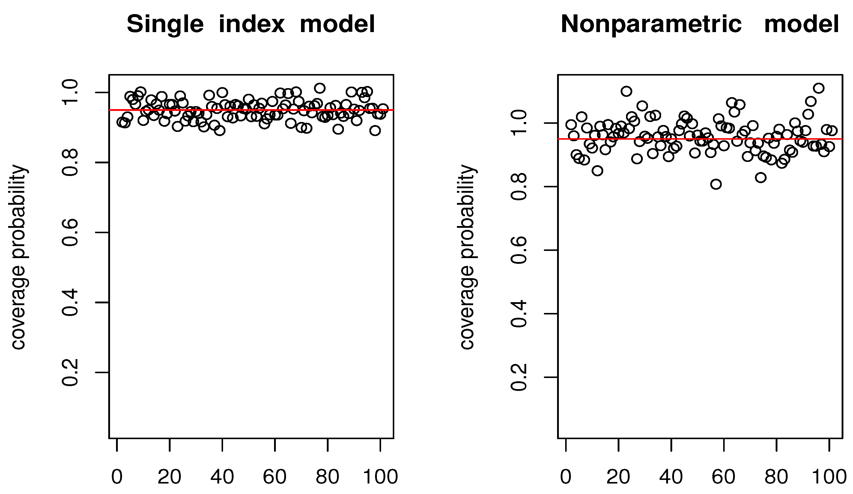
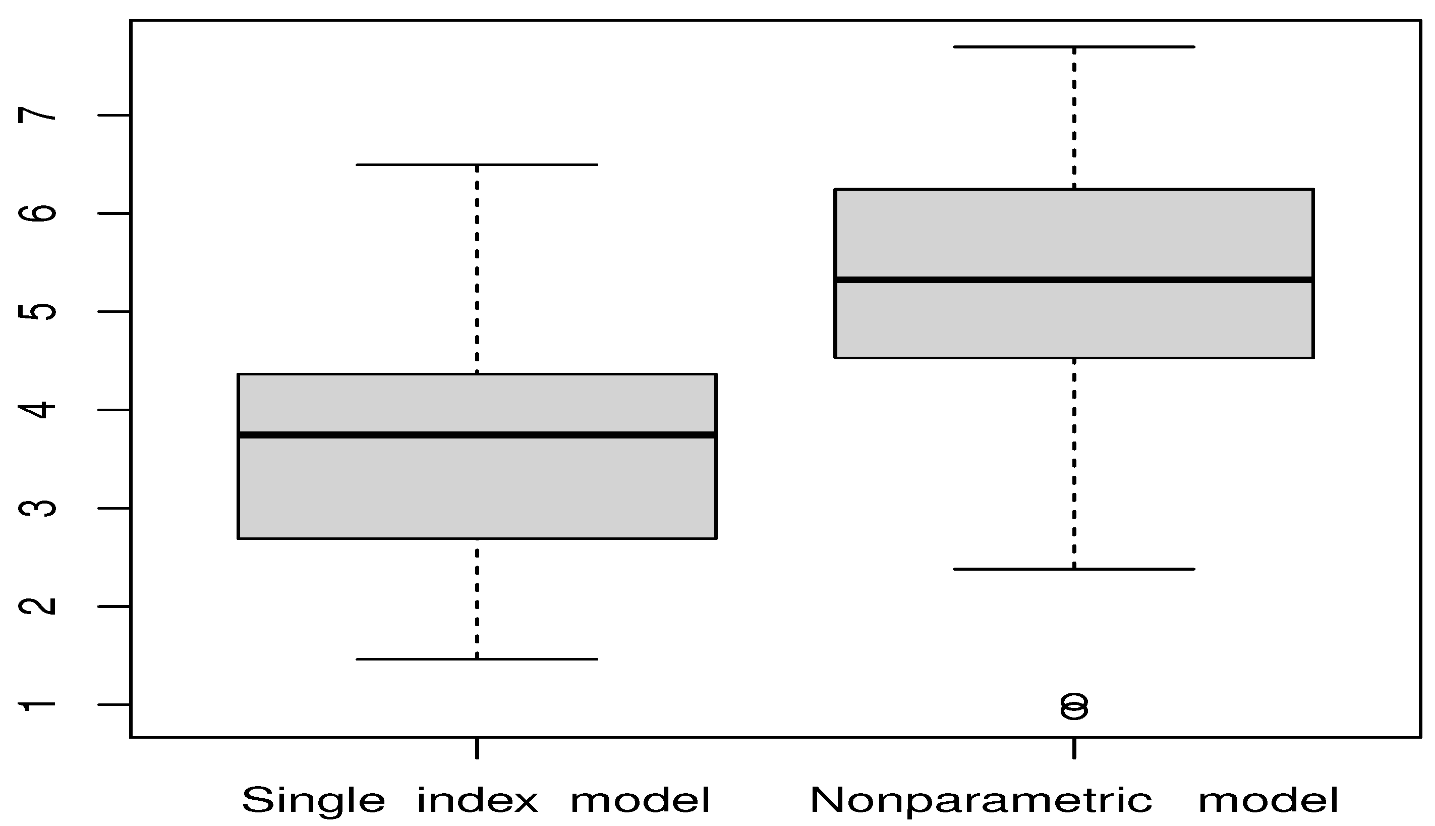
Remark 3. 

Assumption (A1’) characterizes the concentration behaviour of the explanatory variable within small neighborhoods. This is a crucial condition in deriving asymptotic properties, particularly in functional data analysis. The technical conditions in (A3’) and (A4’) facilitate explicit computation of the asymptotic variance. The function ${\beta }_{\theta ,\chi }(·)$ plays a central role in the results, as it determines the precise constant terms appearing in asymptotic expansions (for additional choices of this function, see [63]). Additionally, the condition (A4’-$ii$) ensures the elimination of the bias term in the derivation of asymptotic normality. The sequence $p_n$ introduced in (A7’) is instrumental for applying Doob’s decomposition theorem, which is key in establishing the limiting distribution.

To establish Theorem 2, we rely on the following auxiliary results, proved in Section 8.

Lemma 5. 

Under assumptions (A0), (A1’), (A3’)–(A4’), (A5)–(A6), and (A7’), we have

$$\sqrt{n{\varphi }_{\theta ,\chi }\left(h_n\right)}\left({\widehat{r}}_1(\theta ,\chi )-\mathbb{E}\left[{\widehat{r}}_1(\theta ,\chi )\right]\right)\stackrel{\mathcal{D}}{\to }\mathcal{N}(0,{\sigma }_r^2(\theta ,\chi )).$$

Lemma 6. 

Under assumptions (A1’), (A3’), (A4’-i), (A5)–(A6), and (A7’), we have

$${\widehat{r}}_2(\theta ,\chi )-1\stackrel{\mathbb{P}}{\to }0.$$

Lemma 7. 

Under assumptions (A0), (A1’), and (A2), and if (A4’-$ii$) holds, then we obtain

$$\sqrt{n{\varphi }_{\theta ,\chi }\left(h_n\right)}\left(\mathbb{E}\left[{\widehat{r}}_1(\theta ,\chi )\right]-r(\theta ,\chi ){\widehat{r}}_2(\theta ,\chi )\right)\to 0.$$

Our main result in this section is summarized in the following theorem.

Theorem 2. 

Suppose that the assumptions (A0), (A1’), (A2), (A3’)–(A4’), (A5)–(A6), and (A7’) hold. Then, we have the following asymptotic normality result:

$$\sqrt{n{\varphi }_{\theta ,\chi }\left(h_n\right)}\left({\widehat{r}}_n(\theta ,\chi )-r(\theta ,\chi )\right)\stackrel{\mathcal{D}}{\to }\mathcal{N}(0,{\sigma }_r^2(\theta ,\chi )),$$

where the asymptotic variance is given by

$${\sigma }_r^2(\theta ,\chi )={\displaystyle \frac{c_2{\left(r(\theta ,\chi )\right)}^2}{c_1^2}},$$

with

$$c_l=K^l\left(1\right)-{\int }_0^1{\left(K^l\right)}^{\prime }\left(s\right){\beta }_{\theta ,\chi }\left(s\right)ds,\mathit{for}l=1,2.$$

Proof of Theorem 2. 

We begin by considering the decomposition:

$${\widehat{r}}_n(\theta ,\chi )-r(\theta ,\chi )={\displaystyle \frac{{\widehat{r}}_1(\theta ,\chi )-r(\theta ,\chi ){\widehat{r}}_2(\theta ,\chi )}{{\widehat{r}}_2(\theta ,\chi )}}.$$

(14)

Rewriting the numerator,

$${\widehat{r}}_1(\theta ,\chi )-r(\theta ,\chi ){\widehat{r}}_2(\theta ,\chi )=\left({\widehat{r}}_1(\theta ,\chi )-\mathbb{E}\left[{\widehat{r}}_1(\theta ,\chi )\right]\right)+\left(\mathbb{E}\left[{\widehat{r}}_1(\theta ,\chi )\right]-r(\theta ,\chi ){\widehat{r}}_2(\theta ,\chi )\right).$$

By applying Slutsky’s theorem, one can establish the asymptotic normality of $r(\theta ,\chi )$ by showing that its numerator converges in distribution to $\mathcal{N}(0,{\sigma }_r^2(\theta ,\chi ))$ while its denominator converges in probability to 1.    □

Confidence Interval

Observe in Theorem 2 that the asymptotic variance depends on the unknown function $r(·)$, as well as on the normalization involving ${\varphi }_{\theta ,\chi }\left(h_n\right)$, which cannot be specified directly. Hence, Corollary 3, which provides a minor modification of Theorem 2, yields a formulation that is more suitable for practical use.

As is customary, the conditional variance ${\sigma }_r^2(\theta ,\chi )$ is estimated by

$$\begin{array}{c}\hfill {\sigma }_{r,n}^2(\theta ,\chi )={\displaystyle \frac{c_{2,n}{\left({\widehat{r}}_n(\theta ,\chi )\right)}^2}{c_{1,n}^2}},\end{array}$$

where

$$c_{l,n}=K^l\left(1\right)-{\int }_0^1{\left(K^l\right)}^{\prime }\left(s\right){\beta }_{\theta ,\chi ,n}\left(s\right)ds,\mathrm{for}l=1,2,$$

and

$${\beta }_{\theta ,\chi ,n}\left(s\right)={\displaystyle \frac{{\varphi }_{\theta ,\chi ,n}\left(s{h}_n\right)}{{\varphi }_{\theta ,\chi ,n}\left(h_n\right)}},$$

with

$${\varphi }_{\theta ,\chi ,n}\left(u\right)={\displaystyle \frac{1}{n}}\sum _{i=1}^n{\mathbb{1}}_{\{d_{\theta }(\chi ,X_i)\le u\}}.$$

The following corollary is more or less a straightforward consequence of Theorem 2 and Slutsky’s theorem.

Corollary 3. 

Suppose that the assumptions (A0), (A1’), (A2), (A3’)–(A4’), (A5)–(A6), and (A7’) hold. Then, we have the following asymptotic normality result:

$$\sqrt{n{\varphi }_{\theta ,\chi ,n}\left(h_n\right){\sigma }_{r,n}^{-1}(\theta ,\chi )}\left({\widehat{r}}_n(\theta ,\chi )-r(\theta ,\chi )\right)\stackrel{\mathcal{D}}{\to }\mathcal{N}(0,1).$$

Remark 4. 

Using Corollary 3, the asymptotic $100(1-\alpha )\%$ confidence band for the regression function r is given by

$${\widehat{r}}_n(\theta ,\chi )\pm c_{\alpha }\sqrt{{\displaystyle \frac{{\sigma }_{r,n}(\theta ,\chi )}{n{\varphi }_{\theta ,\chi ,n}\left(h_n\right)}}},$$

where $c_{\alpha }$ is the upper $\alpha /2$ quantile of the distribution of $\mathcal{N}(0,1)$.

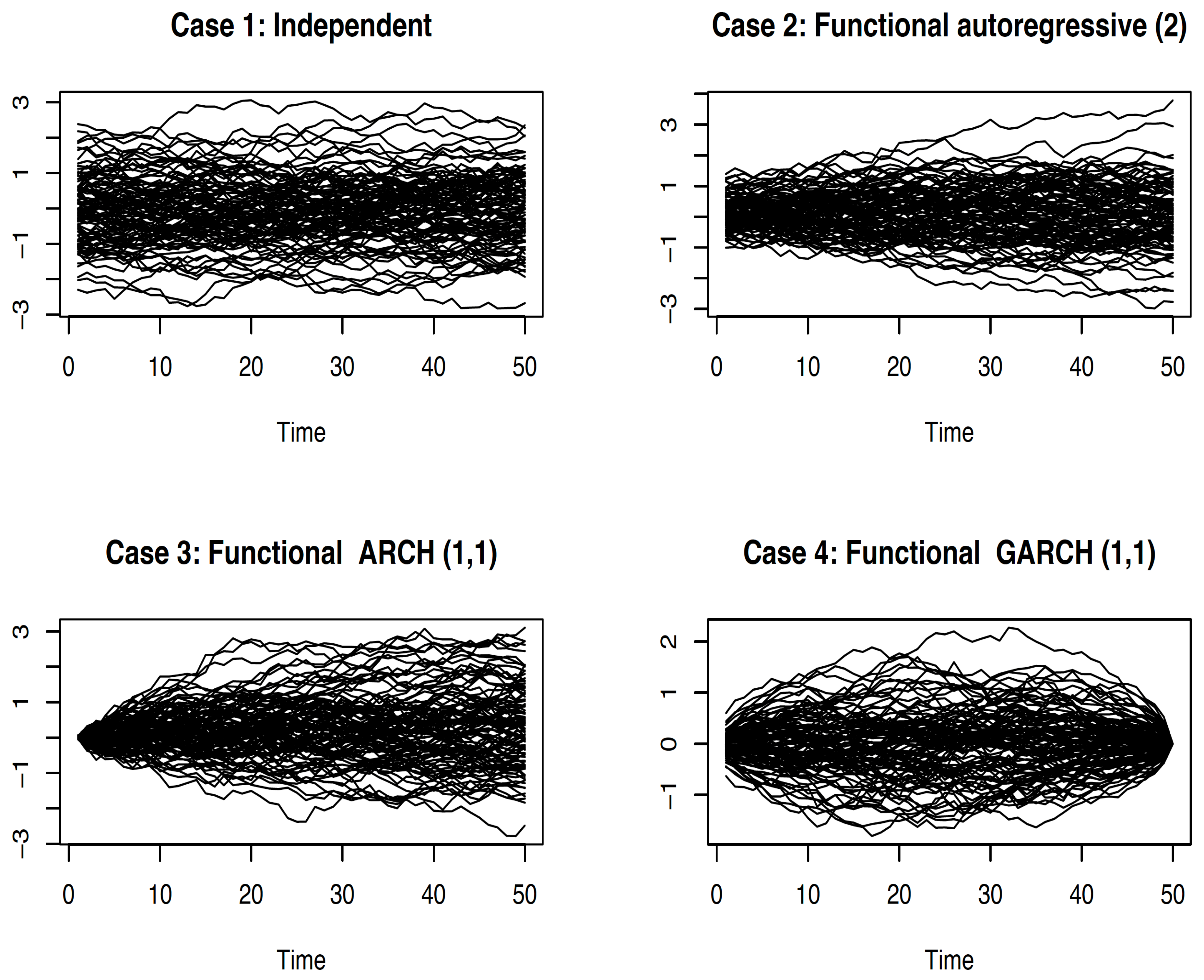
5. Numerical Results

This study examines the performance of an estimator under a variety of theoretical configurations. Four key frameworks form the basis of the analysis: single-index modeling, dependence structures, and the censored functional setting. To conduct this analysis, we construct a functional random variable by generating diverse functional time series data.

The first dataset is generated from a functional autoregressive process of order 2 (FAR(2)), specified as

$$X_i=\sum _{j=1}^2{\int }_0^1\psi (t,s)X_{i-j}\left(s\right)ds+{\epsilon }_i,$$

where

$$\psi (t,s)=exp\left\{\frac{t^2+s^2}{2}\right\}.$$

The second dataset utilizes a functional autoregressive conditional heteroscedastic (FARCH(1,1)) model, defined as

$$X_i\left(t\right)={\sigma }_i\left(t\right){ϵ}_i\left(t\right),$$

where    

$${\sigma }_i^2\left(t\right)=w\left(t\right)+{\int }_0^1\alpha (t,s)X_{i-1}^2\left(s\right)ds,$$

with $w\left(t\right)=0.1t(1-t)$ and $\alpha (t,s)=t(1-t)s(1-s)$.

The third dataset is derived from a functional general autoregressive conditional heteroscedastic (FGARCH(1,1)) model:

$$X_i\left(t\right)={\sigma }_i\left(t\right){ϵ}_i\left(t\right),$$

where    

$${\sigma }_i^2\left(t\right)=w\left(t\right)+{\int }_0^1\alpha (t,s)X_{i-1}^2\left(s\right)ds+{\int }_0^1\alpha (t,s){\sigma }_{i-1}^2\left(s\right)ds.$$

To evaluate the impact of correlation structures on estimation quality, the outcomes from these three types of functional time series are compared with those from an independent (i.i.d.) setting. The different functional covariates are generated using the R package FTSgof; for instance, dgp.far is employed to produce FAR(1)-based regressors, dgp.fgarch creates FGARCH(1,1) processes, and dgp.ou provides i.i.d. data. A visual summary of these generated functional time series appears in Figure 1.

Figure 1. A sample of 100 curves of different functional time series.

In the theoretical segment of this work, we generate the response variable $\left\{Y_i\right\}$ via a functional single-index model of the form

$$Y_i=r⟨\theta ,X_i⟩+{ϵ}_i,\mathrm{where}r\left(z\right)={\displaystyle \frac{2}{2+z^2}}.$$

Here, ${ϵ}_i$ is an independent white noise term (assumed independent of $X_i$) drawn from a normal distribution $\mathcal{N}(0,1)$. The true functional index $\theta$ is selected as the first Karhunen–Loève (KL) [64,65,66] basis function of $\left\{X_i\right\}$. Under this construction, the conditional distribution of $Y_i$ given $X_i$ follows $\mathcal{N}\left(r⟨\theta ,X_i⟩,1\right)$, ensuring that $r⟨\theta ,X_i⟩$ is the true conditional mean.

To introduce censoring, a random variable C is drawn from an exponential distribution $\mathrm{Exp}(1/\lambda )$, where the parameter $\lambda$ controls the censoring rate. High ($\lambda =2$), moderate ($\lambda =0.5$), and low ($\lambda =0.05$) rates correspond to approximate censoring rates of 70–80%, 50–56%, and 4–8%, respectively. The primary objective of this numerical study is to assess the accuracy of the asymptotic normality of the statistic.

$$NT({\chi }_0,\theta )=\sqrt{{\displaystyle \frac{n\widehat{{\varphi }_{\theta }}({\chi }_0,h_n)}{{\widehat{\sigma }}_r^2\left(\widehat{\theta },{\chi }_0\right)}}}\left[{\widehat{r}}_n\left(\widehat{\theta },{\chi }_0\right)-r\left(\theta ,{\chi }_0\right)\right],$$

where ${\chi }_0$ is a fixed conditioning curve (e.g., $X_{i_0}$), and ${\widehat{\sigma }}_r^2\left(\widehat{\theta },{\chi }_0\right)$ is a plug-in estimator of the asymptotic variance,

$$\begin{array}{c}\hfill {\widehat{\sigma }}_r^2(\theta ,\chi )={\displaystyle \frac{\widehat{C_2}(\theta ,\chi ){\left[\widehat{r}(\theta ,\chi )\right]}^2}{{\left[\widehat{C_1}(\theta ,\chi )\right]}^2}},\end{array}$$

(15)

with

$$\widehat{C_{\mathit{\ell }}}(\theta ,\chi )={\displaystyle \frac{1}{n\widehat{{\varphi }_{\theta }}(\chi ,h_n)}}\sum _{i=1}^n{K}_i^{\mathit{\ell }}(\theta ,\chi ),\mathit{\ell }=1,2,$$

and

$$\widehat{{\varphi }_{\theta }}(\chi ,h_n)={\displaystyle \frac{1}{n}}\sum _{i=1}^n\mathbb{1}\left\{\left|⟨\chi -X_i,\theta ⟩\right|<h_n\right\}.$$

Empirically, these estimators are calculated by first selecting both the optimal functional index $\theta$ and bandwidth h via a one-leave-out cross-validation approach:

$$({\theta }_{CV},h_{CV})=arg{\displaystyle \underset{\theta \in {\Theta }_n,h_n\in H_n}{min}}{\displaystyle \frac{1}{n}}\sum _{i=1}^n{\left(Y_i-{\widehat{r}}_n^{-i}\left(\theta ,X_i\right)\right)}^2.$$

The set ${\Theta }_n$ consists of vectors $\theta$ expressible as finite combinations of basis functions $\left\{e_i\right\}$ that span the Hilbert subspace of $\left\{X_i\right\}$, subject to $\parallel \theta \parallel =1$ and certain nontriviality constraints on the coefficients. Meanwhile, $H_n$ is chosen so that the ball of radius $h_n$ around each point $\chi$ contains a fixed number $k\in \{5,15,25,\dots ,55\}$ of neighboring observations. Finally, we generate 100 independent replications of the statistic $NT\left(X_{i_0},{\theta }_{CV}\right)$ and quantify its departure from normality through its empirical bias and variance:

$$\begin{array}{ccc}\hfill \mathrm{Bias}& =& {\displaystyle \frac{1}{100}}\sum _{b=1}^{100}N{T}_b\left(X_{i_0},{\theta }_{CV}\right),\hfill \\ \hfill \mathrm{Var}& =& {\displaystyle \frac{1}{100}}\sum _{b=1}^{100}{\left(N{T}_b\left(X_{i_0},{\theta }_{CV}\right)-\mathrm{Bias}\right)}^2.\hfill \end{array}$$

These measures provide a comprehensive evaluation of how closely $NT({\chi }_0,\theta )$ adheres to its theoretical asymptotic distribution under different levels of censoring and model configurations. The results of bias and the variance are reported in the following Table 1.

Table 1. The bias and the variance for different scenarios.

Functional Time Series Case	n	$\mathit{\lambda }$	Bias	Var
	50	2	0.1436	0.783
	50	0.5	0.230	0.952
	50	0.05	0.111	0.998
	100	2	0.196	0.874
Independent case	100	0.5	0.112	0.831
	100	0.05	0.051	0.967
	350	2	0.121	0.697
	350	0.5	0.101	0.715
	350	0.05	0.022	0.881
	50	2	0.247	0.861
	50	0.5	0.331	0.753
	50	0.05	0.102	0.977
	100	2	0.166	0.699
FAR(1)	100	0.5	0.126	0.702
	100	0.05	0.099	0.913
	350	2	0.135	0.578
	350	0.5	0.881	0.677
	350	0.05	0.085	0.863
	50	2	0.281	0.841
	50	0.5	0.173	0.919
	50	0.05	0.184	0.942
	100	2	0.169	0.768
FARCH(1,1)	100	0.5	0.142	0.823
	100	0.05	0.106	0.893
	350	2	0.117	0.673
	350	0.5	0.110	0.671
	350	0.05	0.098	0.855
	50	2	0.357	1.811
	50	0.5	0.175	1.182
	50	0.05	0.194	1.121
	100	2	0.2126	1.630
FGARCH(1,1)	100	0.5	0.143	1.071
	100	0.05	0.136	1.018
	350	2	0.181	1.541
	350	0.5	0.121	1.131
	350	0.05	0.119	1.009

This study demonstrates that the asymptotic normality of the estimator is shaped by several key elements, including the structure of the functional time series data, the choice of smoothing parameter, censoring, and the functional index. Notably, high levels of dependence and substantial censoring rates can adversely affect the estimator’s performance in finite samples. Evidence supporting this conclusion emerges from a comparison between the results obtained in an i.i.d. setting (with $\lambda =0.05$) and those from an FGARCH(1,1) process (also with $\lambda =0.05$). In the former case, the bias is nearly zero and the variance is close to one, whereas under the FGARCH(1,1) specification, both bias and variance increase substantially. In conclusion, the estimator’s finite-sample performance is notably influenced by the sample size, n. Our simulation studies considered several values of n (namely, 25, 50, 100, 150, 350, and 500). For the sake of brevity, we present results only for $n=50$, 100, and 350, since the other cases yielded similar outcomes. Overall, while the estimator performs adequately even with smaller samples, its effectiveness improves markedly as n increases.

6. Real Data Example

In the second phase of our empirical investigation, we demonstrate how the proposed methodology can be employed in real-world contexts. The study of incomplete functional time series data has garnered significant attention across various applied disciplines, particularly finance, where high-frequency market data frequently exhibit interruptions or extraordinary events. Such interruptions often yield censored observations. To illustrate, we consider the intraday returns of the Nikkei stock index from 1 January 1984, to 31 December 2021. Single-index modeling is extensively used in econometrics because it offers a middle ground between overly rigid parametric models and highly flexible nonparametric alternatives that are challenging to estimate. This approach has been popularized by early studies, such as those in [2,67]. Moreover, financial time series naturally embody the characteristics of quasi-associated functional data. Financial datasets typically display features like high variability, non-normal distributions, excess kurtosis, and irregular volatility. As a result, these series are often modeled using generalized autoregressive conditional heteroskedasticity (GARCH) processes, which provide a clear example of the mathematical formulation of quasi-associated processes (see [17]). Therefore, applying the present model to such complex functional structures enhances its practical applicability. In addition, since trading on this index is suspended whenever prices fall below a specified threshold (an occurrence observed during crisis periods such as the COVID-19 pandemic), the resulting dataset is censored. Throughout the observation period, numerous trading halts led to a substantial censoring rate of approximately 20%. The data, publicly available at https://fred.stlouisfed.org/series/NIKKEI225 (accessed on 5 January 2025), are treated as functional observations by dividing the entire time series into 30-day segments, with each segment reflecting a functional curve for one month. This procedure yields 444 functional observations.

Before conducting our main analysis, we address heteroscedasticity by measuring logarithmic differences. For each month i and day d, we define

$$X_i\left(d\right)=-100log\left({\displaystyle \frac{s\left(d\right)}{s(d-1)}}\right),$$

where $s\left(t\right)$ denotes the daily return. We then set $Y_i={max}_d{X}_{i+1}\left(d\right)$, reflecting the maximum price observed in the subsequent month. The forecasting objective is thus to predict this maximum one month ahead using the functional trajectory of the previous month. We compare two estimation strategies: a single-index estimator $\widehat{r}$ and a nonparametric estimator $\tilde{r}$. The latter employs a kernel-smoothing approach

$$\tilde{r}\left(x\right)=\sum _{i=1}^n{\displaystyle \frac{K\left(h^{-1}d(x,X_i)\right)Y_i}{{\sum }_{j=1}^{n}K\left(h^{-1}d(x,X_j)\right)}},$$

where the bandwidth h and single-index parameter $\theta$ are chosen via cross-validation. The distance $d(·,·)$ is defined through a PCA-based metric, which is suitable for handling discontinuities in the curves.

To evaluate both methods, we estimate confidence intervals by exploiting the asymptotic normality derived in this work. Specifically, we construct a $(1-\zeta )$ confidence interval for $r(\theta ,\chi )$ as

$${\widehat{r}}_n(\theta ,\chi )\pm t_{\zeta /2}{\displaystyle \frac{\widehat{\sigma }(\theta ,\chi )}{\sqrt{n\widehat{{\varphi }_{{\theta }^{*}}}(\chi ,h_n)}}},$$

where $t_{\zeta /2}$ is the $\zeta /2$ upper quantile of the standard normal distribution and $\widehat{\sigma }(\theta ,\chi )$ is an estimate of the asymptotic variance. The performance of these intervals is assessed by their average length and empirical coverage probability. To facilitate comparisons between the two models, we partition the dataset into a training set of 300 observations and a test set of 140 observations, then repeat this split 100 times with different random partitions. The numerical results, including coverage rates and interval lengths, are presented in the subsequent figures.

The results in Figure 2 and Figure 3 indicate that the single-index model substantially outperforms its kernel-based counterpart. In particular, the semi-parametric approach produces narrower confidence intervals while maintaining accurate coverage probabilities. Notably, the average confidence interval length for the estimator ${\widehat{r}}_n$ is 3.56, compared with 5.09 for the kernel estimator $\tilde{r}\left(x\right)$. Moreover, the coverage probabilities associated with ${\widehat{r}}_n$ align more closely with the nominal level than those derived from $\tilde{r}\left(x\right)$.

Figure 2. Comparison of coverage probability of 95% confidence interval.

Figure 3. Comparison of 95% confidence interval-length.

7. Concluding Remarks

This study proposes kernel estimators for regression functions in settings where the data comprise censored time series governed by a functional single-index model. By leveraging the single-index structure, the relationship between the response and covariates is dimensionally reduced, thereby simplifying the model while retaining its ability to capture complex relationships. The proposed methodology employs nonparametric kernel estimation within a quasi-association framework to effectively characterize these dependencies.

We establish that, under mild regularity conditions, the estimators converge uniformly almost surely, and we further demonstrate their asymptotic normality. In addition, we provide practical insights into bandwidth selection and discuss the implications of our theoretical findings for real-world applications. Finally, the proposed methods are evaluated in a comprehensive simulation study, which highlights their robustness and favorable finite-sample performance across various scenarios.

A key issue that has not yet been addressed in this study is how to optimally determine the smoothing parameters so as to minimize the mean square errors (MSEs) of the proposed kernel estimators. This problem is highly relevant within the broader sphere of kernel-based nonparametric estimation, and it merits dedicated investigation. Although this topic is crucial for further enhancing the proposed methodology, we have decided to postpone a comprehensive examination to future work. In that subsequent research, we plan to systematically analyze the selection of smoothing parameters, potentially employing cross-validation or other established methods for optimal parameter choice.

Several other directions also warrant further exploration. The principal drawback of conventional kernel estimators lies in their tendency to incur bias, a challenge that remains central to kernel smoothing. While local linear fitting is theoretically capable of mitigating bias, this issue still requires substantial attention in nonparametric functional data analysis (NFDA). This need becomes especially salient when dealing with complex functional data, where simpler smoothing techniques may produce suboptimal results. Our computational findings illustrate that local linear bias correction significantly enhances estimation performance by reducing overall error. However, incorporating any form of bias correction (CB) into a nonparametric setting demands strong mathematical underpinnings to guarantee control over its asymptotic behavior, a key issue that remains insufficiently studied in the current literature. To our knowledge, no comprehensive investigation of the asymptotic nature of bias correction methods has been conducted in NFDA. We therefore believe this represents an exciting and largely unexplored area for future work. In particular, it would be highly beneficial to assess how the proposed kernel-based approach might be paired with established CB algorithms, such as those introduced by [68,69], which have been shown to improve estimation accuracy in related contexts. Integrating our local linear smoothing framework with these CB algorithms could substantially enhance estimation quality, especially for more complex functional data, by balancing bias reduction against variance control—an essential consideration in nonparametric functional data analysis.

Another natural question is whether our results might be adapted to alternative nonparametric estimation methods, such as wavelet-based estimators, delta sequence estimators [70], $K(·)$-nearest neighbor ($K(·)$NN) estimators [12], and other local linear estimators [71]. These methods, widely used across various fields of functional data analysis, could benefit from the bias correction techniques introduced in this paper. Investigating how these estimators might be extended or combined with our proposed framework could thus reveal valuable synergies, further advancing the capabilities of nonparametric functional data analysis.

Finally, we propose relaxing the stationarity assumption that underpins the current study. Although stationarity is commonly assumed in many functional data models, it may not be appropriate for data exhibiting dynamic or time-varying behavior; see [72]. Extending our approach to accommodate locally stationary functional ergodic processes would be a natural and informative progression; see [73]. Under these more general conditions, the conditional quantile estimator would smoothly vary over time, thereby capturing nonstationary or evolving data structures. Exploring uniform limit theorems for such processes would be an especially promising avenue for future investigation, as it would shed additional light on the asymptotic properties of kernel estimators in more flexible, nonstationary contexts.

8. Proofs

This section is dedicated to presenting the proofs of our findings. The notation previously introduced will continue to be utilized in the ensuing discussions.

The proof Lemma 1 is based on the application of the Bernstein-type inequality for weakly dependent random variables, as proved by [39] in Section 2. Theorem 2.1 stated in the following lemma.

Lemma 8 ([39]). 

Suppose that $X_1,\dots ,X_n$ are real-valued random variables with $\mathrm{I}\mathrm{E}\left(X_i\right)=0$ and $\mathrm{I}\mathrm{P}(|X_i|<M)=1,\mathit{for}\mathit{all}i=1,\dots ,n\mathit{and}\mathit{some}M<\infty .$ Let ${\sigma }_n^2=\mathrm{Var}(X_1+\cdots +X_n)$. Assume, furthermore, that there exist constants $K\ge 1$ and $\beta >0$ such that, for all u-tuples $(s_1,\dots ,s_u)$ and all v-tuples $(t_1,\dots ,t_v)$ with $1\le s_1\le \dots \le s_u\le t_1\le \dots \le t_v\le n$, the following inequality is fulfilled:

$$|\mathrm{Cov}(X_{s_1}\cdots X_{s_u},X_{t_1}\cdots X_{t_v})|\le K^2{M}^{u+v}vexp\left(-\beta (t_1-s_u)\right).$$

Then

$$\mathrm{I}\mathrm{P}\left(\sum _{i=1}^n{X}_i\ge t\right)\le exp\left(-{\displaystyle \frac{t^2/2}{A_n+B^{1/3}{t}^{5/3}}}\right),$$

where $A_n$ can be chosen as any value greater than or equal to ${\sigma }_n^2$, and

$$B=\left({\displaystyle \frac{16n{K}^2}{9A_n(1-e^{-\beta })}}\vee 1\right){\displaystyle \frac{2(K\vee M)}{1-e^{-\beta }}}.$$

Proof of Lemma 1. 

Next, let us consider the following decomposition:

$$\begin{array}{cc}\hfill {\displaystyle \underset{\chi \in S_{\mathcal{H}}}{sup}}& {\displaystyle \underset{\theta \in {\Theta }_{\mathcal{H}}}{sup}}\left|{\tilde{r}}_1(\theta ,\chi )-\mathrm{I}\mathrm{E}\left[{\tilde{r}}_1(\theta ,\chi )\right]\right|\hfill \\ \hfill \le & {\displaystyle \underset{F_1}{{\displaystyle \underbrace{\underset{\chi \in S_{\mathcal{H}}}{sup}\underset{\theta \in {\Theta }_{\mathcal{H}}}{sup}\left|{\tilde{r}}_1(\theta ,\chi )-{\tilde{r}}_1(\theta ,{\chi }_{k\left(\chi \right)})\right|}}}}\hfill \\ & +{\displaystyle \underset{F_2}{{\displaystyle \underbrace{\underset{\chi \in S_{\mathcal{H}}}{sup}\underset{\theta \in {\Theta }_{\mathcal{H}}}{sup}\left|{\tilde{r}}_1(\theta ,{\chi }_{k\left(\chi \right)})-{\tilde{r}}_1(t_{j\left(\theta \right)},{\chi }_{k\left(\chi \right)})\right|}}}}\hfill \\ & +{\displaystyle \underset{F_3}{{\displaystyle \underbrace{\underset{\chi \in S_{\mathcal{H}}}{sup}\underset{\theta \in {\Theta }_{\mathcal{H}}}{sup}\left|{\tilde{r}}_1(t_{j\left(\theta \right)},{\chi }_{k\left(\chi \right)})-\mathrm{I}\mathrm{E}\left[{\tilde{r}}_1(t_{j\left(\theta \right)},{\chi }_{k\left(\chi \right)})\right]\right|}}}}\hfill \\ & +{\displaystyle \underset{F_4}{{\displaystyle \underbrace{\underset{\chi \in S_{\mathcal{H}}}{sup}\underset{\theta \in {\Theta }_{\mathcal{H}}}{sup}\left|\mathrm{I}\mathrm{E}\left[{\tilde{r}}_1(t_{j\left(\theta \right)},{\chi }_{k\left(\chi \right)})\right]-\mathrm{I}\mathrm{E}\left[{\tilde{r}}_1(\theta ,{\chi }_{k\left(\chi \right)})\right]\right|}}}}\hfill \\ & +{\displaystyle \underset{F_5}{{\displaystyle \underbrace{\underset{\chi \in S_{\mathcal{H}}}{sup}\underset{\theta \in {\Theta }_{\mathcal{H}}}{sup}\left|\mathrm{I}\mathrm{E}\left[{\tilde{r}}_1(\theta ,{\chi }_{k\left(\chi \right)})\right]-\mathrm{I}\mathrm{E}\left[{\tilde{r}}_1(\theta ,\chi )\right]\right|}}}}.\hfill \end{array}$$

Since both $F_1$ and $F_5$ can be treated in the same way, we only deal with $F_1$. Indeed, by (A3-$\left(ii\right)$) and Cauchy Schwartz’s inequality, we have

$$\begin{array}{cc}\hfill {\displaystyle \underset{\chi \in S_{\mathcal{H}}}{sup}}& {\displaystyle \underset{\theta \in {\Theta }_{\mathcal{H}}}{sup}}\left|{\tilde{r}}_1(\theta ,\chi )-{\tilde{r}}_1(\theta ,{\chi }_{k\left(\chi \right)})\right|\hfill \\ \hfill \le & {\displaystyle \frac{1}{n}}{\displaystyle \underset{\chi \in S_{\mathcal{H}}}{sup}}{\displaystyle \underset{\theta \in {\Theta }_{\mathcal{H}}}{sup}}\sum _{i=1}^n{\displaystyle \frac{{\delta }_i|Y_i|}{\overline{G}\left(Y_i\right)}}\left|{\displaystyle \frac{K_i(\theta ,\chi )}{\mathrm{I}\mathrm{E}\left[K_1(\theta ,\chi )\right]}}-{\displaystyle \frac{K_i(\theta ,{\chi }_{k\left(\chi \right)})}{\mathrm{I}\mathrm{E}\left[K_1(\theta ,{\chi }_{k\left(\chi \right)})\right]}}\right|\hfill \\ \hfill \le & {\displaystyle \frac{1}{n\varphi \left(h_n\right)}{\displaystyle \underset{\chi \in S_{\mathcal{H}}}{sup}}{\displaystyle \underset{\theta \in {\Theta }_{\mathcal{H}}}{sup}}\sum _{i=1}^n\frac{{\mathbb{1}}_{\{Y_i^0\le C_i\}}|Y_i^0|}{\overline{G}\left(Y_i^0\right)}\left|K_i(\theta ,\chi )-K_i(\theta ,{\chi }_{k\left(\chi \right)})\right|}\hfill \\ \hfill \le & {\displaystyle \frac{C{\tau }_F}{\overline{G}\left({\tau }_F\right)}}{\displaystyle \underset{\chi \in S_{\mathcal{H}}}{sup}}{\displaystyle \underset{\theta \in {\Theta }_{\mathcal{H}}}{sup}}{\displaystyle \frac{\parallel \theta \parallel ·\parallel \chi -{\chi }_{k\left(\chi \right)}\parallel }{h_n\varphi \left(h_n\right)}}\hfill \\ \hfill \le & {\displaystyle \frac{C{\tau }_F}{\overline{G}\left({\tau }_F\right)}}{\displaystyle \frac{l_n}{\varphi \left(h_n\right)}}.\hfill \end{array}$$

Thus, by assumption (A4-($ii$)), since $l_n=O\left({\displaystyle \frac{logn}{n}}\right)$, by Jensen’s inequality, we see that n goes to infinity

$$\begin{array}{c}\hfill F_5\le F_1=O\left(\sqrt{{\displaystyle \frac{log{d}_n^{S_{\mathcal{H}}}+log{d}_n^{{\Theta }_{\mathcal{H}}}}{n\varphi \left(h_n\right)}}}\right).\end{array}$$

(16)

Analogously, dealing with $F_2$ and $F_4$ in the same way, one may easily obtain

$$\begin{array}{cc}\hfill {\displaystyle \underset{\chi \in S_{\mathcal{H}}}{sup}}& {\displaystyle \underset{\theta \in {\Theta }_{\mathcal{H}}}{sup}}\left|{\tilde{r}}_1(\theta ,\chi )-{\tilde{r}}_1(\theta ,{\chi }_{k\left(\chi \right)})\right|\hfill \\ \hfill \le & {\displaystyle \frac{1}{n\varphi \left(h_n\right)}{\displaystyle \underset{\chi \in S_{\mathcal{H}}}{sup}}{\displaystyle \underset{\theta \in {\Theta }_{\mathcal{H}}}{sup}}\sum _{i=1}^n\frac{{\mathbb{1}}_{\{Y_i^0\le C_i\}}|Y_i^0|}{\overline{G}\left(Y_i^0\right)}\left|K_i(\theta ,\chi )-K_i(t_{j\left(\theta \right)},\chi )\right|}\hfill \\ \hfill \le & {\displaystyle \frac{C{\tau }_F}{\overline{G}\left({\tau }_F\right)}}{\displaystyle \underset{\chi \in S_{\mathcal{H}}}{sup}}{\displaystyle \underset{\theta \in {\Theta }_{\mathcal{H}}}{sup}}{\displaystyle \frac{\parallel \chi \parallel ·\parallel \theta -t_{j\left(\theta \right)}\parallel }{h_n\varphi \left(h_n\right)}}\hfill \\ \hfill \le & {\displaystyle \frac{C{\tau }_F}{\overline{G}\left({\tau }_F\right)}}{\displaystyle \frac{l_n}{\varphi \left(h_n\right)}}\hfill \\ \hfill =& O\left({\displaystyle \frac{logn}{n\varphi \left(h_n\right)}}\right).\hfill \end{array}$$

Hence, we conclude that

$$\begin{array}{c}\hfill F_4\le F_2=O\left(\sqrt{{\displaystyle \frac{log{d}_n^{S_{\mathcal{H}}}+log{d}_n^{{\Theta }_{\mathcal{H}}}}{n\varphi \left(h_n\right)}}}\right).\end{array}$$

(17)

Now, our focus turns to the upper bound of the term $F_3$. Firstly, we express

$$\begin{array}{ccc}\hfill \mathrm{I}\mathrm{P}\left(F_3>ϵ\right)& \le & d_n^{S_{\mathcal{H}}}{d}_n^{{\Theta }_{\mathcal{H}}}{\displaystyle \underset{1\le k\le d_n^{S_{\mathcal{H}}}}{max}}{\displaystyle \underset{1\le j\le d_n^{{\Theta }_{\mathcal{H}}}}{max}}\mathrm{I}\mathrm{P}\left(\left|{\tilde{r}}_N(t_{j\left(\theta \right)},{\chi }_{k\left(\chi \right)})-\mathrm{I}\mathrm{E}\left[{\tilde{r}}_N(t_{j\left(\theta \right)},{\chi }_{k\left(\chi \right)})\right]\right|>ϵ\right)\hfill \\ & \le & d_n^{S_{\mathcal{H}}}{d}_n^{{\Theta }_{\mathcal{H}}}{\displaystyle \underset{1\le k\le d_n^{S_{\mathcal{H}}}}{max}}{\displaystyle \underset{1\le j\le d_n^{{\Theta }_{\mathcal{H}}}}{max}}\mathrm{I}\mathrm{P}\left(\left|\sum _{i=1}^n{\Psi }_i\right|>ϵ\right),\hfill \end{array}$$

where

$${\Psi }_i={\displaystyle \frac{1}{n\mathrm{I}\mathrm{E}\left[K_1(t_{j\left(\theta \right)},{\chi }_{k\left(\chi \right)})\right]}}\phi (X_i,Y_i),$$

with

$$\phi (X_i,Y_i)={\displaystyle \frac{{\delta }_i{Y}_i}{\overline{G}\left(Y_i\right)}}{K}_i(t_{j\left(\theta \right)},{\chi }_{k\left(\chi \right)})-\mathrm{I}\mathrm{E}\left[{\displaystyle \frac{{\delta }_1{Y}_1}{\overline{G}\left(Y_1\right)}}{K}_1(t_{j\left(\theta \right)},{\chi }_{k\left(\chi \right)})\right],1\le i\le n.$$

Clearly, we have

$$\begin{array}{ccc}\hfill \mathrm{I}\mathrm{E}\left({\Psi }_i\right)& =& 0\hfill \\ \hfill {\parallel \phi \parallel }_{\infty }& \le & {2C\parallel K\parallel }_{\infty }and\mathrm{Lip}\left(\phi \right)\le 2C{h}_n^{-1}\mathrm{Lip}\left(K\right).\hfill \end{array}$$

It is important to highlight that the Kallabis and Neumann inequality in [39] relies on the asymptotic evaluation of both quantities:

$$\mathrm{Var}\left(\sum _{i=1}^n{\Psi }_i\right)\mathrm{and}\mathrm{Cov}\left({\Psi }_{s_1}\cdots {\Psi }_{s_u},{\Psi }_{t_1}\cdots {\Psi }_{t_v}\right),\forall (s_1\dots s_u)\in {\mathrm{I}\mathrm{N}}^u;\forall (t_1\dots t_v)\in {\mathrm{I}\mathrm{N}}^v.$$

We begin by studying the variance term:

$$\begin{array}{ccc}\hfill \mathrm{Var}\left(\sum _{i=1}^n{\Psi }_i\right)& =& n\mathrm{Var}\left({\Psi }_1\right)+\sum _{i=1}^n\sum _{{\displaystyle \underset{i\ne l}{l=1}}}^n\left|\mathrm{Cov}\left({\Psi }_i,{\Psi }_l\right)\right|\hfill \\ & =:& J_{1,n}+J_{2,n}.\hfill \end{array}$$

(18)

For $J_{1,n}$, we have

$$\begin{array}{ccc}\hfill J_{1,n}& =& {\displaystyle \frac{n}{{\left(n\mathrm{I}\mathrm{E}\left[K_1(t_{j\left(\theta \right)},{\chi }_{k\left(\chi \right)})\right]\right)}^2}}\mathrm{Var}\left(\phi (X_i,Y_i)\right)\hfill \\ & \le & O\left({\displaystyle \frac{1}{n{\left(\mathrm{I}\mathrm{E}\left[K_1(t_{j\left(\theta \right)},{\chi }_{k\left(\chi \right)})\right]\right)}^2}}\mathrm{I}\mathrm{E}\left[K_1^2(t_{j\left(\theta \right)},{\chi }_{k\left(\chi \right)})\right]\right).\hfill \end{array}$$

Since $K(·)$ is bounded with support $[0,1]$, Assumption (A1) implies

$$\mathrm{I}\mathrm{E}\left[K_1^2(\theta ,\chi )\right]\le C{\varphi }_{\theta ,\chi }\left(h_n\right),\forall (\theta ,\chi )\in \mathcal{H}\times \mathcal{H}.$$

Hence,

$$\begin{array}{ccc}\hfill J_{1,n}& =& O\left({\displaystyle \frac{1}{n{\varphi }_{\theta ,\chi }\left(h_n\right)}}\right).\hfill \end{array}$$

(19)

We will now focus on the quantity $J_{2,n}$, and thus we have

$$J_{2,n}=\sum _{i=1}^n\sum _{{\displaystyle \underset{i\ne l}{l=1}}}^n\left|\mathrm{Cov}\left({\Psi }_i,{\Psi }_l\right)\right|.$$

To deal with this last quantity, we merely need to split it into

$$\begin{array}{ccc}\hfill J_{2,n}& =& \sum _{i=1}^n\sum _{{\displaystyle \underset{0<|l-i|\le m_n}{l=1}}}^n\left|\mathrm{Cov}\left({\Psi }_i,{\Psi }_l\right)\right|\hfill \\ & & +\sum _{i=1}^n\sum _{{\displaystyle \underset{m_n+1\le |l-i|\le n-1}{l=1}}}^n\left|\mathrm{Cov}\left({\Psi }_i,{\Psi }_l\right)\right|\hfill \\ & =:& J_{2,n}^{\prime }+J_{2,n}^{″},\hfill \end{array}$$

where $m_n$ is a sequence of natural numbers going to infinity as $n\to \infty$. First, we deal with $J_{2,n}^{\prime }$, so

$$\begin{array}{ccc}\hfill J_{2,n}^{\prime }& \le & {\displaystyle \frac{Cn}{{\left(n\mathrm{I}\mathrm{E}\left[K_1(t_{j\left(\theta \right)},{\chi }_{k\left(\chi \right)})\right]\right)}^2}}\sum _{{\displaystyle \underset{0<|l-i|\le m_n}{l=1}}}^n\left|\mathrm{Cov}\left(K_i(t_{j\left(\theta \right)},{\chi }_{k\left(\chi \right)}),K_l(t_{j\left(\theta \right)},{\chi }_{k\left(\chi \right)})\right)\right|\hfill \\ & \le & {\displaystyle \frac{C}{n{\left(\mathrm{I}\mathrm{E}\left[K_1(t_{j\left(\theta \right)},{\chi }_{k\left(\chi \right)})\right]\right)}^2}}\sum _{{\displaystyle \underset{0<|l-i|\le m_n}{j=1}}}^n\left|\mathrm{I}\mathrm{E}\left[K_i\left(t_{j\left(\theta \right)}{\chi }_{k\left(\chi \right)}\right)K_l(t_{j\left(\theta \right)},{\chi }_{k\left(\chi \right)})\right]\right|.\hfill \end{array}$$

Assumptions (A1), (A3), and (A6) allow us to write

$$\begin{array}{ccc}\hfill \left|\mathrm{I}\mathrm{E}\left[K_i\left(t_{j\left(\theta \right)}{\chi }_{k\left(\chi \right)}\right)K_l(t_{j\left(\theta \right)},{\chi }_{k\left(\chi \right)})\right]\right|& \le & C\left[\mathrm{I}\mathrm{P}(X_i,X_l)\in B_{\theta }(\chi ,h_n)\times B_{\theta }(\chi ,h_n)\right]\hfill \\ & =& O\left({\varphi }_{\theta ,\chi }{\left(h_n\right)}^2\right).\hfill \end{array}$$

Therefore,

$$\begin{array}{ccc}\hfill J_{2,n}^{\prime }& =& O\left({\displaystyle \frac{m_n}{n}}\right).\hfill \end{array}$$

Second, by applying the quasi-association of the sequence $(X_i,Y_i)$, we have by assumption (A5):

$$\begin{array}{ccc}\hfill J_{2,n}^{″}& \le & {\displaystyle \frac{C}{{\left(n\mathrm{I}\mathrm{E}\left[K_1(t_{j\left(\theta \right)},{\chi }_{k\left(\chi \right)})\right]\right)}^2}}\sum _{i=1}^n\sum _{{\displaystyle \underset{|l-i|\ge m_n+1}{l=1}}}^n{\lambda }_{i,l}.\hfill \end{array}$$

(20)

Thus, since $|l-i|\ge m_n+1>m_n$

$$\begin{array}{ccc}\hfill J_{2,n}^{″}& \le & O\left({\displaystyle \frac{1}{{\left(n{\varphi }_{\theta ,\chi }\left(h_n\right)\right)}^2}}{n}^2{\lambda }_{m_n}\right)=O\left({\varphi }_{\theta ,\chi }{\left(h_n\right)}^{-2}{e}^{-a{m}_n}\right).\hfill \end{array}$$

So,

$$\begin{array}{ccc}\hfill J_{2,n}=J_{2,n}^{\prime }+J_{2,n}^{″}& \le & C\left({\displaystyle \frac{m_n}{n}}+{\varphi }_{\theta ,\chi }{\left(h_n\right)}^{-2}{e}^{-a{m}_n}\right)\hfill \\ & =& O\left({\displaystyle \frac{m_n}{n}}+{\displaystyle \frac{1}{{\varphi }_{\theta ,\chi }{\left(h_n\right)}^2{e}^{a{m}_n}}}\right).\hfill \end{array}$$

Choosing ${\displaystyle m_n=\frac{1}{a}log\left(\frac{n}{{\varphi }_{\theta ,\chi }{\left(h_n\right)}^2}\right),a>0}$, we have

$$\begin{array}{ccc}\hfill J_{2,n}& =& O\left(o\left(1\right)+{\displaystyle \frac{1}{n}}\right)\hfill \\ & =& o\left(1\right).\hfill \end{array}$$

(21)

Combining (19) and (21), we get

$$\begin{array}{ccc}\hfill \mathrm{Var}\left(\sum _{i=1}^n{\Psi }_i\right)& =& O\left({\displaystyle \frac{1}{n{\varphi }_{\theta ,\chi }\left(h_n\right)}}\right).\hfill \end{array}$$

(22)

Now, we treat the covariance $\mathrm{Cov}\left({\Psi }_{s_1}\cdots {\Psi }_{s_u},{\Psi }_{t_1}\cdots {\Psi }_{t_v}\right),\forall (s_1\dots s_u)\in {\mathrm{I}\mathrm{N}}^u;$$\forall (t_1\dots t_v)\in {\mathrm{I}\mathrm{N}}^v$.

To proceed, we consider the following cases:

• If $t_1=s_u$, we obtain

  $$\begin{array}{ccc}\hfill \left|\mathrm{Cov}\left({\Psi }_{s_1}\cdots {\Psi }_{s_u},{\Psi }_{t_1}\cdots {\Psi }_{t_v}\right)\right|& \le & {\left({\displaystyle \frac{{C\parallel K\parallel }_{\infty }}{n\mathrm{I}\mathrm{E}\left[K_1(t_{j\left(\theta \right)},{\chi }_{k\left(\chi \right)})\right]}}\right)}^{u+v}\mathrm{I}\mathrm{E}\left[K_1^2(t_{j\left(\theta \right)},{\chi }_{k\left(\chi \right)})\right]\hfill \\ & \le & {\varphi }_{\theta ,\chi }\left(h_n\right){\left({\displaystyle \frac{C}{n{\varphi }_{\theta ,\chi }\left(h_n\right)}}\right)}^{u+v}.\hfill \end{array}$$

  (23)
• If $t_1>s_u$, we apply the quasi-association condition to show

  $$\begin{array}{cc}\hfill |\mathrm{Cov}& \left({\Psi }_{s_1}\cdots {\Psi }_{s_u},{\Psi }_{t_1}\cdots {\Psi }_{t_v}\right)|\hfill \\ \hfill \le & {\left({\displaystyle \frac{C{h}_n^{-1}\mathrm{Lip}\left(K\right))}{n\mathrm{I}\mathrm{E}\left[K_1(t_{j\left(\theta \right)},{\chi }_{k\left(\chi \right)})\right]}}\right)}^2{\left({\displaystyle \frac{{2\parallel K\parallel }_{\infty }}{n\mathrm{I}\mathrm{E}\left[K_1(t_{j\left(\theta \right)},{\chi }_{k\left(\chi \right)})\right]}}\right)}^{u+v-2}\sum _{i=1}^u\sum _{j=1}^v{\lambda }_{s_i,t_j}\hfill \\ \hfill \le & h_n^{-2}{\left({\displaystyle \frac{C}{n{\varphi }_{\theta ,\chi }\left(h_n\right)}}\right)}^{u+v}v{\lambda }_{t_1-s_u}\hfill \\ \hfill \le & h_n^{-2}{\left({\displaystyle \frac{C}{n{\varphi }_{\theta ,\chi }\left(h_n\right)}}\right)}^{u+v}v{e}^{-a(t_1-s_u)}.\hfill \end{array}$$

  (24)

Conversely, we have

$$\begin{array}{cc}\hfill |\mathrm{Cov}& \left({\Psi }_{s_1}\cdots {\Psi }_{s_u},{\Psi }_{t_1}\cdots {\Psi }_{t_v}\right)|\hfill \\ \hfill \le & {\left({\displaystyle \frac{{2C\parallel K\parallel }_{\infty }}{n\mathrm{I}\mathrm{E}\left[K_1(t_{j\left(\theta \right)},{\chi }_{k\left(\chi \right)})\right]}}\right)}^{u+v-2}\left|\mathrm{I}\mathrm{E}\left({\Psi }_{s_u}{\Psi }_{t_1}\right)\right|\hfill \\ \hfill \le & {\left({\displaystyle \frac{{2C\parallel K\parallel }_{\infty }}{n\mathrm{I}\mathrm{E}\left[K_1(t_{j\left(\theta \right)},{\chi }_{k\left(\chi \right)})\right]}}\right)}^{u+v}{\displaystyle \underset{i\ne l}{sup}}\mathrm{I}\mathrm{P}\left((X_i,X_l)\in {\mathcal{B}}_{\theta }(\chi ,h_n)\times {\mathcal{B}}_{\theta }(\chi ,h_n)\right)\hfill \\ \hfill \le & {\varphi }_{\theta ,\chi }{\left(h_n\right)}^2{\left({\displaystyle \frac{C}{n{\varphi }_{\theta ,\chi }\left(h_n\right)}}\right)}^{u+v}.\hfill \end{array}$$

(25)

Now, taking a $\rho$-power of (24), $(1-\rho )$-power of (25), under assumption (A7)-$\left(i\right)$, we obtain an upper bound of the three terms as follows

$$\begin{array}{ccc}\hfill \left|\mathrm{Cov}\left({\Psi }_{s_1}\cdots {\Psi }_{s_u},{\Psi }_{t_1}\cdots {\Psi }_{t_v}\right)\right|& \le & {\varphi }_{\theta ,\chi }\left(h_n\right){\left({\displaystyle \frac{C}{n{\varphi }_{\theta ,\chi }\left(h_n\right)}}\right)}^{u+v}v{e}^{-a\rho (t_1-s_u)}.\hfill \end{array}$$

Therefore, the conditions of Theorem 2.1 of [39] are fulfilled by the variables ${\Psi }_i,i=1,\dots ,n$, where

$$K_n={\displaystyle \frac{C}{n\sqrt{{\varphi }_{\theta ,\chi }\left(h_n\right)}}},M_n={\displaystyle \frac{C}{n{\varphi }_{\theta ,\chi }\left(h_n\right)}}\mathrm{and}{A}_n=\mathrm{Var}\left(\sum _{i=1}^n{\Psi }_i\right)=O\left({\displaystyle \frac{1}{n{\varphi }_{\theta ,\chi }\left(h_n\right)}}\right).$$

As a result, it follows that

$$\begin{array}{cc}\hfill \mathrm{I}\mathrm{P}& \left(\left|\sum _{i=1}^n{\Psi }_i\right|>\eta {\left(\frac{log{d}_n^{S_{\mathcal{H}}}+log{d}_n^{{\Theta }_{\mathcal{H}}}}{n\varphi \left(h_n\right)}\right)}^{1/2}\right)\hfill \\ & \le exp\left\{-{\displaystyle \frac{{\eta }^2\left(\frac{log\left(d_n^{S_{\mathcal{H}}}{d}_n^{{\Theta }_{\mathcal{H}}}\right)}{n\varphi \left(h_n\right)}\right)}{C{\left(n\varphi \left(h_n\right)\right)}^{-1}+{\left({\left(n\varphi \left(h_n\right)\right)}^{-1}{\eta }^5{\left(\frac{log\left(d_n^{S_{\mathcal{H}}}{d}_n^{{\Theta }_{\mathcal{H}}}\right)}{n\varphi \left(h_n\right)}\right)}^{5/2}\right)}^{1/3}}}\right\}\hfill \\ & \le exp\left\{-{\displaystyle \frac{{\eta }^{2}log\left(d_n^{S_{\mathcal{H}}}{d}_n^{{\Theta }_{\mathcal{H}}}\right)}{C+n\varphi \left(h_n\right){\left(C{\left(n\varphi \left(h_n\right)\right)}^{-1}{\eta }^5{\left(\frac{log\left(d_n^{S_{\mathcal{H}}}{d}_n^{{\Theta }_{\mathcal{H}}}\right)}{n\varphi \left(h_n\right)}\right)}^{5/2}\right)}^{1/3}}}\right\}\hfill \\ & \le exp\left\{-{\displaystyle \frac{{\eta }^{2}log\left(d_n^{S_{\mathcal{H}}}{d}_n^{{\Theta }_{\mathcal{H}}}\right)}{C+{\eta }^{5/3}{\left({\left(n\varphi \left(h_n\right)\right)}^{4/5}\left(\frac{log\left(d_n^{S_{\mathcal{H}}}{d}_n^{{\Theta }_{\mathcal{H}}}\right)}{n\varphi \left(h_n\right)}\right)\right)}^{5/6}}}\right\}\hfill \\ & \le exp\left\{-{\displaystyle \frac{{\eta }^{2}log\left(d_n^{S_{\mathcal{H}}}{d}_n^{{\Theta }_{\mathcal{H}}}\right)}{C+{\eta }^{5/3}{\left(\frac{{log}^5\left(d_n^{S_{\mathcal{H}}}{d}_n^{{\Theta }_{\mathcal{H}}}\right)}{\left(n\varphi \left(h_n\right)\right)}\right)}^{1/6}}}\right\}.\hfill \end{array}$$

From assumption (A7)-$\left(ii\right)$, we get

$$\begin{array}{cc}\hfill \mathrm{I}\mathrm{P}& \left(\left|\sum _{i=1}^n{\Psi }_i\right|>\eta {\left(\frac{log{d}_n^{S_{\mathcal{H}}}+log{d}_n^{{\Theta }_{\mathcal{H}}}}{n\varphi \left(h_n\right)}\right)}^{1/2}\right)\hfill \\ & \le exp\left\{-{\displaystyle \frac{{\eta }^{2}log\left(d_n^{S_{\mathcal{H}}}{d}_n^{{\Theta }_{\mathcal{H}}}\right)}{C+o\left(1\right)}}\right\}={\left(d_n^{S_{\mathcal{H}}}{d}_n^{{\Theta }_{\mathcal{H}}}\right)}^{-C^{\prime }{\eta }^2}.\hfill \end{array}$$

An appropriate choice of $\eta$ ensures the existence of some real $\beta =C^{\prime }{\eta }^2$ with $\beta >2$:

$$\begin{array}{c}\hfill \mathrm{I}\mathrm{P}\left(\left|{\widehat{r}}_1(t_{j\left(\theta \right)},{\chi }_{k\left(\chi \right)})-\mathrm{I}\mathrm{E}\left[{\widehat{r}}_1(t_{j\left(\theta \right)},{\chi }_{k\left(\chi \right)})\right]\right|>\eta \sqrt{{\displaystyle \frac{log{d}_n^{S_{\mathcal{H}}}+log{d}_n^{{\Theta }_{\mathcal{H}}}}{n\varphi \left(h_n\right)}}}\right)\\ \hfill \le C^{\prime }{\left(d_n^{S_{\mathcal{H}}}{d}_n^{{\Theta }_{\mathcal{H}}}\right)}^{-\beta }.\end{array}$$

Therefore,

$$\begin{array}{ccc}\hfill \mathrm{I}\mathrm{P}\left(F_3>ϵ\right)& \le & C^{\prime }{\left(d_n^{S_{\mathcal{H}}}{d}_n^{{\Theta }_{\mathcal{H}}}\right)}^{1-\beta }.\hfill \end{array}$$

Assumption (A5)-$\left(ii\right)$ implies

$$\begin{array}{c}\hfill F_3=O_{a.co.}\left(\sqrt{{\displaystyle \frac{log{d}_n^{S_{\mathcal{H}}}+log{d}_n^{{\Theta }_{\mathcal{H}}}}{n\varphi \left(h_n\right)}}}\right).\end{array}$$

(26)

Finally, results (26), (17), and (16) complete the proof of Lemma 3. □

Proof of Lemma 2. 

Since

$$\mathrm{I}\mathrm{E}\left[{\widehat{r}}_2(\theta ,\chi )\right]=\mathrm{I}\mathrm{E}\left[{\widehat{r}}_2(t_{j\left(\theta \right)},{\chi }_{k\left(\chi \right)})\right]=1,$$

we can write

$$\begin{array}{ccc}\hfill {\displaystyle \underset{\chi \in S_{\mathcal{H}}}{sup}}{\displaystyle \underset{\theta \in {\Theta }_{\mathcal{H}}}{sup}}\left|{\widehat{r}}_2(\theta ,\chi )-\mathrm{I}\mathrm{E}\left[{\widehat{r}}_2(\theta ,\chi )\right]\right|& \le & {\displaystyle \underset{\chi \in S_{\mathcal{H}}}{sup}}{\displaystyle \underset{\theta \in {\Theta }_{\mathcal{H}}}{sup}}\left|{\widehat{r}}_2(\theta ,\chi )-{\widehat{r}}_2(\theta ,{\chi }_{k\left(\chi \right)})\right|\hfill \\ & +& {\displaystyle \underset{\chi \in S_{\mathcal{H}}}{sup}}{\displaystyle \underset{\theta \in {\Theta }_{\mathcal{H}}}{sup}}\left|{\widehat{r}}_2(\theta ,{\chi }_{k\left(\chi \right)})-{\widehat{r}}_2(t_{j\left(\theta \right)},{\chi }_{k\left(\chi \right)})\right|\hfill \\ & +& {\displaystyle \underset{\chi \in S_{\mathcal{H}}}{sup}}{\displaystyle \underset{\theta \in {\Theta }_{\mathcal{H}}}{sup}}\left|{\widehat{r}}_2(t_{j\left(\theta \right)},{\chi }_{k\left(\chi \right)})-1\right|.\hfill \end{array}$$

(27)

For the first and the second terms on the right-hand side of the previous inequality, we use the Hölder continuity condition of $K(·)$ (in view of (A3-$\left(ii\right)$)) and the Cauchy–Schwartz inequality to obtain

$$\begin{array}{ccc}\hfill {\displaystyle \underset{\chi \in S_{\mathcal{H}}}{sup}}{\displaystyle \underset{\theta \in {\Theta }_{\mathcal{H}}}{sup}}\left|{\widehat{r}}_2(\theta ,\chi )-{\widehat{r}}_2(\theta ,{\chi }_{k\left(\chi \right)})\right|& =& O\left(\sqrt{{\displaystyle \frac{log{d}_n^{S_{\mathcal{H}}}+log{d}_n^{{\Theta }_{\mathcal{H}}}}{n\varphi \left(h_n\right)}}}\right),\hfill \end{array}$$

(28)

and

$$\begin{array}{ccc}\hfill {\displaystyle \underset{\chi \in S_{\mathcal{H}}}{sup}}{\displaystyle \underset{\theta \in {\Theta }_{\mathcal{H}}}{sup}}\left|{\widehat{r}}_2(\theta ,{\chi }_{k\left(\chi \right)})-{\widehat{r}}_2(t_{j\left(\theta \right)},{\chi }_{k\left(\chi \right)})\right|& =& O\left(\sqrt{{\displaystyle \frac{log{d}_n^{S_{\mathcal{H}}}+log{d}_n^{{\Theta }_{\mathcal{H}}}}{n\varphi \left(h_n\right)}}}\right).\hfill \end{array}$$

(29)

Clearly, by the Lipschitz property of $K(·)$ imposed in (A3-$\left(ii\right)$) and Cauchy–Schwartz inequality, we can write

$$\begin{array}{cc}\hfill {\displaystyle \underset{\chi \in S_{\mathcal{H}}}{sup}}& {\displaystyle \underset{\theta \in {\Theta }_{\mathcal{H}}}{sup}}\left|{\widehat{r}}_2(\theta ,\chi )-{\widehat{r}}_2(\theta ,{\chi }_{k\left(\chi \right)})\right|\hfill \\ \hfill \le & {\displaystyle \frac{C}{{\varphi }_{\theta ,\chi }\left(h_n\right)}}{\displaystyle \underset{\theta \in {\Theta }_{\mathcal{H}}}{sup}}{\displaystyle \frac{1}{n}}\sum _{i=1}^n\left|K\left({\displaystyle \frac{d_{\theta }(\chi ,X_i)}{h_n}}\right)-K\left({\displaystyle \frac{d_{\theta }({\chi }_{k\left(\chi \right)},X_i)}{h_n}}\right)\right|\hfill \\ \hfill \le & {\displaystyle \frac{C}{h_n{\varphi }_{\theta ,\chi }\left(h_n\right)}}{\displaystyle \underset{\theta \in {\Theta }_{\mathcal{H}}}{sup}}{\displaystyle \frac{1}{n}}\sum _{i=1}^n||⟨\theta ,\chi -X_i⟩|-\left|⟨\theta ,{\chi }_{k\left(\chi \right)}-X_i⟩\right||\hfill \\ \hfill \le & C{\displaystyle \underset{\theta \in {\Theta }_{\mathcal{H}}}{sup}}{\displaystyle \frac{\parallel \theta \parallel ·\parallel \chi -{\chi }_{k\left(\chi \right)}\parallel }{h_n\varphi \left(h_n\right)}}\hfill \\ \hfill \le & C{\displaystyle \frac{l_n}{\varphi \left(h_n\right)}}.\hfill \end{array}$$

Because $l_n=O\left({\displaystyle \frac{logn}{n}}\right)$, we obtain for n an infinitely large value

$$\begin{array}{ccc}\hfill {\displaystyle \underset{\chi \in S_{\mathcal{H}}}{sup}}{\displaystyle \underset{\theta \in {\Theta }_{\mathcal{H}}}{sup}}\left|{\widehat{r}}_2(\theta ,\chi )-{\widehat{r}}_2(\theta ,{\chi }_{k\left(\chi \right)})\right|& =& O\left({\displaystyle \frac{logn}{n\varphi \left(h_n\right)}}\right)\hfill \\ & =& o\left(\sqrt{{\displaystyle \frac{log{d}_n^{S_{\mathcal{H}}}+log{d}_n^{{\Theta }_{\mathcal{H}}}}{n\varphi \left(h_n\right)}}}\right).\hfill \end{array}$$

(30)

Similarly, following the same steps leading to (30), we have

$$\begin{array}{ccc}\hfill {\displaystyle \underset{\chi \in S_{\mathcal{H}}}{sup}}{\displaystyle \underset{\theta \in {\Theta }_{\mathcal{H}}}{sup}}\left|{\widehat{r}}_2(\theta ,{\chi }_{k\left(\chi \right)})-{\widehat{r}}_2(t_{j\left(\theta \right)},{\chi }_{k\left(\chi \right)})\right|& =& O\left({\displaystyle \frac{logn}{n\varphi \left(h_n\right)}}\right)\hfill \\ & =& o\left(\sqrt{{\displaystyle \frac{log{d}_n^{S_{\mathcal{H}}}+log{d}_n^{{\Theta }_{\mathcal{H}}}}{n\varphi \left(h_n\right)}}}\right).\hfill \end{array}$$

(31)

For the last term on the right-hand side of (27), we have

$$\begin{array}{cc}\hfill \mathrm{I}\mathrm{P}& \left({\displaystyle \underset{\chi \in S_{\mathcal{H}}}{sup}}{\displaystyle \underset{\theta \in {\Theta }_{\mathcal{H}}}{sup}}\left|{\widehat{r}}_2(t_{j\left(\theta \right)},{\chi }_{k\left(\chi \right)})-1\right|>\eta {\left(\frac{log{d}_n^{S_{\mathcal{H}}}+log{d}_n^{{\Theta }_{\mathcal{H}}}}{n\varphi \left(h_n\right)}\right)}^{1/2}\right)\hfill \\ & \le \mathrm{I}\mathrm{P}\left({\displaystyle \underset{k=1,\dots ,d_n^{S_{\mathcal{H}}}}{max}}{\displaystyle \underset{j=1,\dots ,d_n^{{\Theta }_{\mathcal{H}}}}{max}}\left|{\widehat{r}}_2(t_{j\left(\theta \right)},{\chi }_{k\left(\chi \right)})-1\right|>\eta {\left({\displaystyle \frac{log{d}_n^{S_{\mathcal{H}}}+log{d}_n^{{\Theta }_{\mathcal{H}}}}{n\varphi \left(h_n\right)}}\right)}^{1/2}\right)\hfill \\ & \le C{d}_n^{S_{\mathcal{H}}}{d}_n^{{\Theta }_{\mathcal{H}}}\mathrm{I}\mathrm{P}\left(\left|{\widehat{r}}_2(t_{j\left(\theta \right)},{\chi }_{k\left(\chi \right)})-1\right|>\eta {\left({\displaystyle \frac{log{d}_n^{S_{\mathcal{H}}}+log{d}_n^{{\Theta }_{\mathcal{H}}}}{n\varphi \left(h_n\right)}}\right)}^{1/2}\right).\hfill \end{array}$$

It worth nothing that the probability

$$\mathrm{I}\mathrm{P}\left(\left|{\widehat{r}}_2(t_{j\left(\theta \right)},{\chi }_{k\left(\chi \right)})-1\right|>\eta {\left({\displaystyle \frac{log{d}_n^{S_{\mathcal{H}}}+log{d}_n^{{\Theta }_{\mathcal{H}}}}{n\varphi \left(h_n\right)}}\right)}^{1/2}\right),$$

represents a special case of the following probability when we take $Y\equiv 1$:

$$\mathrm{I}\mathrm{P}\left(\left|{\tilde{r}}_1(t_{j\left(\theta \right)},{\chi }_{k\left(\chi \right)})-\mathrm{I}\mathrm{E}\left[{\tilde{r}}_1(t_{j\left(\theta \right)},{\chi }_{k\left(\chi \right)})\right]\right|>\eta {\left({\displaystyle \frac{log{d}_n^{S_{\mathcal{H}}}+log{d}_n^{{\Theta }_{\mathcal{H}}}}{n\varphi \left(h_n\right)}}\right)}^{1/2}\right).$$

Thus,

$$\begin{array}{c}\hfill \mathrm{I}\mathrm{P}\left({\displaystyle \underset{\chi \in S_{\mathcal{H}}}{sup}}{\displaystyle \underset{\theta \in {\Theta }_{\mathcal{H}}}{sup}}\left|{\widehat{r}}_2(t_{j\left(\theta \right)},{\chi }_{k\left(\chi \right)})-1\right|>\eta \sqrt{{\displaystyle \frac{log{d}_n^{S_{\mathcal{H}}}+log{d}_n^{{\Theta }_{\mathcal{H}}}}{n\varphi \left(h_n\right)}}}\right)\\ \hfill \le C{\left(d_n^{S_{\mathcal{H}}}{d}_n^{{\Theta }_{\mathcal{H}}}\right)}^{1-\beta }.\end{array}$$

Therefore, by assumption (A5)-$\left(ii\right)$,

$$\begin{array}{c}\hfill {\displaystyle \underset{\chi \in S_{\mathcal{H}}}{sup}}{\displaystyle \underset{\theta \in {\Theta }_{\mathcal{H}}}{sup}}\left|{\widehat{r}}_2(t_{j\left(\theta \right)},{\chi }_{k\left(\chi \right)})-1\right|=O\left(\sqrt{{\displaystyle \frac{log{d}_n^{S_{\mathcal{H}}}+log{d}_n^{{\Theta }_{\mathcal{H}}}}{n\varphi \left(h_n\right)}}}\right).\end{array}$$

(32)

Combining this last result together with results (31) and (30) ends the proof of the lemma. □

Proof of Corollary 1. 

Observe that if

$${\displaystyle \underset{\chi \in S_{\mathcal{H}}}{inf}}{\displaystyle \underset{\theta \in {\Theta }_{\mathcal{H}}}{inf}}\left|{\widehat{r}}_2(\theta ,\chi )\right|\le \frac{1}{2},$$

then there must exist some $\chi \in S_{\mathcal{H}}$ and $\theta \in {\Theta }_{\mathcal{H}}$ such that

$${\displaystyle \underset{\chi \in S_{\mathcal{H}}}{sup}}{\displaystyle \underset{\theta \in {\Theta }_{\mathcal{H}}}{sup}}\left|1-{\widehat{r}}_2(\theta ,\chi )\right|>\frac{1}{2}.$$

Hence, it follows that

$$\mathbb{P}\left({\displaystyle \underset{\chi \in S_{\mathcal{H}}}{inf}}{\displaystyle \underset{\theta \in {\Theta }_{\mathcal{H}}}{inf}}\left|{\widehat{r}}_2(\theta ,\chi )\right|\le \frac{1}{2}\right)\le \mathbb{P}\left({\displaystyle \underset{\chi \in S_{\mathcal{H}}}{sup}}{\displaystyle \underset{\theta \in {\Theta }_{\mathcal{H}}}{sup}}\left|1-{\widehat{r}}_2(\theta ,\chi )\right|>\frac{1}{2}\right).$$

By invoking Lemma 2, the proof of the corollary is thus established. □

Proof of Lemma 3. 

First, observe that the difference $\left|{\widehat{r}}_1(\theta ,\chi )-{\tilde{r}}_1(\theta ,\chi )\right|$ can be written as

$$\begin{array}{cc}\hfill \left|{\widehat{r}}_1(\theta ,\chi )-{\tilde{r}}_1(\theta ,\chi )\right|& ={\displaystyle \frac{1}{n\mathbb{E}\left[K_1(\theta ,\chi )\right]}}\sum _{i=1}^n\left|\left({\displaystyle \frac{{\delta }_i{Y}_i}{{\overline{G}}_n\left(Y_i\right)}}-{\displaystyle \frac{{\delta }_i{Y}_i}{\overline{G}\left(Y_i\right)}}\right)K_i(\theta ,\chi )\right|\hfill \\ \hfill & ={\displaystyle \frac{1}{n\mathbb{E}\left[K_1(\theta ,\chi )\right]}}\sum _{i=1}^n\left|\left({\displaystyle \frac{{\mathbf{1}}_{\{Y_i^0\le C_i\}}{Y}_i^0}{{\overline{G}}_n\left(Y_i^0\right)}}-{\displaystyle \frac{{\mathbf{1}}_{\{Y_i^0\le C_i\}}{Y}_i^0}{\overline{G}\left(Y_i^0\right)}}\right)K_i(\theta ,\chi )\right|.\hfill \end{array}$$

Since ${\delta }_i={\mathbf{1}}_{\{Y_i^0\le C_i\}}$, we may factor out $Y_i^0{K}_i(\theta ,\chi )$ and obtain

$$\left|{\widehat{r}}_1(\theta ,\chi )-{\tilde{r}}_1(\theta ,\chi )\right|\le {\displaystyle \frac{1}{n\mathbb{E}\left[K_1(\theta ,\chi )\right]}}\sum _{i=1}^n|Y_i^0{K}_i(\theta ,\chi )|\left|{\displaystyle \frac{{\overline{G}}_n\left(Y_i^0\right)-\overline{G}\left(Y_i^0\right)}{{\overline{G}}_n\left(Y_i^0\right)\overline{G}\left(Y_i^0\right)}}\right|.$$

Noting that $Y_i^0\le {\tau }_F$ and employing ${\overline{G}}_n\left(t\right)\ge {\overline{G}}_n\left({\tau }_F\right)$ and $\overline{G}\left(t\right)\ge \overline{G}\left({\tau }_F\right)$ for $t<{\tau }_F$, one obtains

$$\left|{\widehat{r}}_1(\theta ,\chi )-{\tilde{r}}_1(\theta ,\chi )\right|\le {\displaystyle \frac{{\tau }_F}{{\overline{G}}_n\left({\tau }_F\right)\overline{G}\left({\tau }_F\right)}}{\displaystyle \underset{t<{\tau }_F}{sup}}\left|{\overline{G}}_n\left(t\right)-\overline{G}\left(t\right)\right|{\displaystyle \frac{1}{n\mathbb{E}\left[K_1(\theta ,\chi )\right]}}\sum _{i=1}^n{K}_i(\theta ,\chi ).$$

Recognizing that ${\displaystyle \frac{1}{n\mathbb{E}\left[K_1(\theta ,\chi )\right]}\sum _{i=1}^n{K}_i(\theta ,\chi )={\widehat{r}}_2(\theta ,\chi )}$, so we have

$$\left|{\widehat{r}}_1(\theta ,\chi )-{\tilde{r}}_1(\theta ,\chi )\right|\le {\widehat{r}}_2(\theta ,\chi ){\displaystyle \frac{{\tau }_F}{{\overline{G}}_n\left({\tau }_F\right)\overline{G}\left({\tau }_F\right)}}{\displaystyle \underset{t<{\tau }_F}{sup}}\left|{\overline{G}}_n\left(t\right)-\overline{G}\left(t\right)\right|.$$

One can further split ${\widehat{r}}_2(\theta ,\chi )$ as ${\widehat{r}}_2(\theta ,\chi )-1+1$, which yields

$$\begin{array}{ccc}\hfill \left|{\widehat{r}}_1(\theta ,\chi )-{\tilde{r}}_1(\theta ,\chi )\right|& \le & ({\widehat{r}}_2(\theta ,\chi )-1){\displaystyle \frac{{\tau }_F}{{\overline{G}}_n\left({\tau }_F\right)\overline{G}\left({\tau }_F\right)}}{\displaystyle \underset{t<{\tau }_F}{sup}}\left|{\overline{G}}_n\left(t\right)-\overline{G}\left(t\right)\right|\hfill \\ & & +{\displaystyle \frac{{\tau }_F}{{\overline{G}}_n\left({\tau }_F\right)\overline{G}\left({\tau }_F\right)}}{\displaystyle \underset{t<{\tau }_F}{sup}}\left|{\overline{G}}_n\left(t\right)-\overline{G}\left(t\right)\right|.\hfill \end{array}$$

Consequently,

$$\begin{array}{cc}\hfill {\displaystyle \underset{\chi \in S_{\mathcal{H}}}{sup}}& {\displaystyle \underset{\theta \in {\Theta }_{\mathcal{H}}}{sup}}\left|{\widehat{r}}_1(\theta ,\chi )-{\tilde{r}}_1(\theta ,\chi )\right|\hfill \\ \hfill \le & {\displaystyle \underset{\chi \in S_{\mathcal{H}}}{sup}}{\displaystyle \underset{\theta \in {\Theta }_{\mathcal{H}}}{sup}}\left|{\widehat{r}}_1(\theta ,\chi )-1\right|{\displaystyle \frac{{\tau }_F}{{\overline{G}}_n\left({\tau }_F\right)\overline{G}\left({\tau }_F\right)}}{\displaystyle \underset{t<{\tau }_F}{sup}}\left|{\overline{G}}_n\left(t\right)-\overline{G}\left(t\right)\right|\hfill \\ & +{\displaystyle \frac{{\tau }_F}{{\overline{G}}_n\left({\tau }_F\right)\overline{G}\left({\tau }_F\right)}}{\displaystyle \underset{t<{\tau }_F}{sup}}\left|{\overline{G}}_n\left(t\right)-\overline{G}\left(t\right)\right|.\hfill \end{array}$$

Next, by combining Lemma 2 with the result of [61], we know

$${\displaystyle \underset{t<{\tau }_F}{sup}}\left|{\overline{G}}_n\left(t\right)-\overline{G}\left(t\right)\right|=O\left(\sqrt{{\displaystyle \frac{{log}_2\left(n\right)}{n}}}\right).$$

Since ${\overline{G}}_n\left({\tau }_F\right)\overline{G}\left({\tau }_F\right)$ converges asymptotically to ${\left(\overline{G}\left({\tau }_F\right)\right)}^2$ as $n\to \infty$, and

$${\displaystyle \frac{{log}_2\left(n\right)}{n}}=o\left({\displaystyle \frac{log\left(n\right)}{n\varphi \left(h_n\right)}}\right)\mathrm{by}\left(\mathrm{A}4\right)-\left(\mathrm{ii}\right),$$

it follows that

$${\displaystyle \underset{\chi \in S_{\mathcal{H}}}{sup}}{\displaystyle \underset{\theta \in {\Theta }_{\mathcal{H}}}{sup}}\left|{\widehat{r}}_1(\theta ,\chi )-{\tilde{r}}_1(\theta ,\chi )\right|=o\left(\sqrt{{\displaystyle \frac{log\left(d_n^{S_{\mathcal{H}}}\right)+log\left(d_n^{{\Theta }_{\mathcal{H}}}\right)}{n\varphi \left(h_n\right)}}}\right).$$

This completes the argument. □

Proof of Lemma 4. 

Leveraging the stationarity assumption, conditioning on $⟨\theta ,X_1⟩$, and noting that

$$\mathbb{E}\left[{\mathbb{1}}_{\{Y_1^0\le C_1\}}|Y_1^0\right]=\overline{G}\left(Y_1^0\right),$$

we deduce the following sequence of identities:

$$\begin{array}{cc}\hfill \mathbb{E}& \left[{\tilde{r}}_1(\theta ,\chi )\right]-r(\theta ,\chi )\hfill \\ & ={\displaystyle \frac{1}{\mathbb{E}\left[K_1(\theta ,\chi )\right]}}\mathbb{E}\left[\frac{{\delta }_1{Y}_1}{\overline{G}\left(Y_1\right)}{K}_1(\theta ,\chi )\right]-r(\theta ,\chi )\hfill \\ & =\mathbb{E}\left[\frac{\mathbb{E}\left[\frac{{\delta }_1{Y}_1}{\overline{G}\left(Y_1\right)}|⟨\theta ,X_1⟩\right]K_1(\theta ,\chi )-r(\theta ,\chi )\mathbb{E}\left[K_1(\theta ,\chi )\right]}{\mathbb{E}\left[K_1(\theta ,\chi )\right]}\right]\hfill \\ & =\mathbb{E}\left[\frac{\mathbb{E}\left[\frac{Y_1^0}{\overline{G}\left(Y_1^0\right)}\mathbb{E}\{{\mathbb{1}}_{\{Y_1^0\le C_1\}}\mid Y_1^0\}|⟨\theta ,X_1⟩\right]K_1(\theta ,\chi )-r(\theta ,\chi )\mathbb{E}\left[K_1(\theta ,\chi )\right]}{\mathbb{E}\left[K_1(\theta ,\chi )\right]}\right]\hfill \\ & =\mathbb{E}\left[\frac{r(\theta ,X_1)K_1(\theta ,\chi )-r(\theta ,\chi )\mathbb{E}\left[K_1(\theta ,\chi )\right]}{\mathbb{E}\left[K_1(\theta ,\chi )\right]}\right]\hfill \\ & ={\displaystyle \frac{1}{\mathbb{E}\left[K_1(\theta ,\chi )\right]}}\mathbb{E}\left[K_1(\theta ,\chi ){\mathbb{1}}_{\left\{B_{\theta }(\chi ,h_n)\right\}}\left(X_1\right)\left(r(\theta ,X_1)-r(\theta ,\chi )\right)\right].\hfill \end{array}$$

Under the Lipschitz condition (Assumption (A2)), there exists a constant C such that

$${\mathbb{1}}_{B_{\theta }(\chi ,h_n)}\left(X_1\right)\left|r(\theta ,X_1)-r(\theta ,\chi )\right|\le C{d}_{\theta }{(\chi ,X_1)}^{\gamma }\le C{h}_n^{\gamma }.$$

Hence, uniformly in both $\chi$ and $\theta$, it follows that

$${\displaystyle \underset{\chi \in S_{\mathcal{H}}}{sup}}{\displaystyle \underset{\theta \in {\Theta }_{\mathcal{H}}}{sup}}\left|\mathbb{E}\left[{\tilde{r}}_1(\theta ,\chi )\right]-r(\theta ,\chi )\right|=O\left(h_n^{\gamma }\right).$$

This completes the proof. □

Proof of Lemma 5. 

Below, we restate some auxiliary results from [63] that will be instrumental in our subsequent proofs:

$${\displaystyle \frac{1}{{\varphi }_{\theta ,\chi }\left(h_n\right)}}\mathrm{I}\mathrm{E}\left[K_1^l(\theta ,\chi )\right]⟶c_l=K^l\left(1\right)-{\int }_0^1{\left(K^l\right)}^{\prime }\left(s\right){\beta }_{\theta ,\chi }\left(s\right)ds,\mathrm{as}n\to \infty ,l\in \{1,2\}.$$

(33)

For any $\theta ,\chi \in \mathcal{H}$, define

$$Z_{ni}(\theta ,\chi )={\displaystyle \frac{\sqrt{{\varphi }_{\theta ,\chi }\left(h_n\right)}}{\sqrt{n}\mathrm{I}\mathrm{E}\left[K_1(\theta ,\chi )\right]}}\left({\displaystyle \frac{{\delta }_i{Y}_i}{{\overline{G}}_n\left(Y_i\right)}}{K}_i(\theta ,\chi )-\mathrm{I}\mathrm{E}\left[{\displaystyle \frac{{\delta }_1{Y}_1}{{\overline{G}}_n\left(Y_1\right)}}{K}_1(\theta ,\chi )\right]\right),$$

and let

$$S_n:=\sum _{i=1}^n{Z}_{ni}(\theta ,\chi ).$$

It follows immediately that

$$S_n=\sqrt{n{\varphi }_{\theta ,\chi }\left(h_n\right)}\left({\widehat{r}}_1(\theta ,\chi )-\mathrm{I}\mathrm{E}\left[{\widehat{r}}_1(\theta ,\chi )\right]\right).$$

Thus, our goal now is to show

$$S_n\stackrel{\mathcal{D}}{\to }\mathcal{N}\left(0,{\sigma }_r(\theta ,\chi )\right),$$

(34)

where $\stackrel{\mathcal{D}}{\to }$ denotes convergence in distribution and ${\sigma }_r(\theta ,\chi )$ is the limiting variance.

Our strategy for establishing the asymptotic behavior of $S_n$ is based on Doob’s methodology (see [74], pp. 228–231), which decomposes $S_n$ into a predictable component and a fluctuation component. This decomposition illuminates both the main stochastic fluctuations (controlled via conditional expectations) and the predictable variation (analyzed via limit theorems), providing a structured way to precisely characterize the limiting distribution of $S_n$. We introduce two sequences of natural numbers $p=p_n$ and $q=q_n$, both tending to infinity as $n\to \infty$, with the additional restriction that $q=o\left(p\right)$. Using these, we decompose $S_n$ as follows:

$$S_n=T_n+T_n^{\prime }+{\zeta }_k,$$

where

$$T_n=\sum _{j=1}^k{\eta }_j,T_n^{\prime }=\sum _{j=1}^k{\xi }_j,{\zeta }_k=\sum _{i=k(p+q)+1}^n{Z}_{ni}(\theta ,\chi ),$$

and the index sets are defined by

$$\begin{array}{ccc}\hfill I_j& =& \left\{\right(j-1\left)\right(p+q)+1,\dots ,(j-1\left)\right(p+q)+p\},\hfill \\ \hfill J_j& =& \left\{\right(j-1\left)\right(p+q)+p+1,\dots ,j(p+q\left)\right\},\hfill \end{array}$$

with

$${\eta }_j={\displaystyle \sum _{i\in I_j}}{Z}_{ni}(\theta ,\chi ),{\xi }_j={\displaystyle \sum _{i\in J_j}}{Z}_{ni}(\theta ,\chi ).$$

Let $k=⌊n/(p+q)⌋$. It then follows that

$${\displaystyle \frac{pq}{n}}\to 1\mathrm{and}{\displaystyle \frac{kq}{n}}\to 0,\mathrm{as}n\to \infty .$$

The main asymptotic properties we need to establish can be summarized as verifying the following two statements:

$$\mathrm{I}\mathrm{E}\left[{\left(T_n^{\prime }\right)}^2\right]+\mathrm{I}\mathrm{E}\left[{\zeta }_k^2\right]⟶0,$$

(35)

and

$$T_n\stackrel{\mathcal{D}}{\to }\mathcal{N}\left(0,{\sigma }_r^2(\theta ,\chi )\right).$$

(36)

These results collectively imply the convergence in (34).

• Proof of (35):
• Proof of $\mathrm{I}\mathrm{E}\left[{\left(T_n^{\prime }\right)}^2\right]\to 0$: Using stationarity and basic covariance bounds, we have

  $$\begin{array}{ccc}\hfill \mathrm{I}\mathrm{E}{\left(T_n^{\prime }\right)}^2& =& k\mathrm{Var}\left({\xi }_1\right)+2{\displaystyle \sum _{1\le i<j\le k}}|\mathrm{Cov}({\xi }_i,{\xi }_j)|\hfill \end{array}$$

  (37)
• Bound for $k\mathrm{Var}\left({\xi }_1\right)$:

  $$\begin{array}{ccc}\hfill k\mathrm{Var}\left({\xi }_1\right)& \le & kq\mathrm{Var}\left(Z_{n1}\right)+2k{\displaystyle \sum _{1\le i<j\le q}}|\mathrm{Cov}(Z_{ni},Z_{nj})|.\hfill \end{array}$$

  (38)

From the definition of the $Z_{n1}$, conditioning w.r.t $⟨\theta ,X_1⟩$, and again the fact

$$\mathrm{I}\mathrm{E}\left[{\mathbb{1}}_{\{Y_1^0\le C_1\}}|Y_1^0\right]=\overline{G}\left(Y_1^0\right),$$

and the fact $G_n\left(t\right)\to G\left(t\right)$; for instance, see [75]. We obtain

$$\begin{array}{cc}\hfill \mathrm{Var}& \left(Z_{n1}\right)={\left(\frac{\sqrt{{\varphi }_{\theta ,\chi }\left(h_n\right)}}{\sqrt{n}\mathrm{I}\mathrm{E}\left[K_1(\theta ,\chi )\right]}\right)}^2\mathrm{Var}\left(\frac{{\delta }_1{Y}_1}{{\overline{G}}_n\left(Y_1\right)}{K}_1(\theta ,\chi )-\mathrm{I}\mathrm{E}\left[\frac{{\delta }_1{Y}_1}{{\overline{G}}_n\left(Y_1\right)}{K}_1(\theta ,\chi )\right]\right)\hfill \\ \hfill =& {\left({\displaystyle \frac{\sqrt{{\varphi }_{\theta ,\chi }\left(h_n\right)}}{\sqrt{n}\mathrm{I}\mathrm{E}\left[K_1(\theta ,\chi )\right]}}\right)}^2\mathrm{Var}\left({\displaystyle \frac{{\delta }_1{Y}_1}{{\overline{G}}_n\left(Y_1\right)}}{K}_1(\theta ,\chi )\right)\hfill \\ \hfill =& {\left({\displaystyle \frac{\sqrt{{\varphi }_{\theta ,\chi }\left(h_n\right)}}{\sqrt{n}\mathrm{I}\mathrm{E}\left[K_1(\theta ,\chi )\right]}}\right)}^2\mathrm{Var}\left({\displaystyle \frac{\mathrm{I}\mathrm{E}\left[{\displaystyle \frac{{\delta }_1{Y}_1}{\overline{G}\left(Y_1\right)}|⟨\theta ,X_1⟩}\right]}{{\overline{G}}_n\left(Y_1\right)}}{K}_1(\theta ,\chi )\right)\hfill \\ \hfill \\ \hfill =& {\left({\displaystyle \frac{\sqrt{{\varphi }_{\theta ,\chi }\left(h_n\right)}}{\sqrt{n}\mathrm{I}\mathrm{E}\left[K_1(\theta ,\chi )\right]}}\right)}^2\mathrm{Var}\left({\displaystyle \frac{\mathrm{I}\mathrm{E}\left[{\displaystyle \frac{Y_1^0}{\overline{G}\left(Y_1^0\right)}\mathrm{I}\mathrm{E}\left\{{\mathbb{1}}_{\{Y_1^0\le C_1\}}|Y_1^0\right\}|⟨\theta ,X_1⟩}\right]}{{\overline{G}}_n\left(Y_1\right)}}{K}_1(\theta ,\chi )\right)\hfill \\ \hfill \\ \hfill =& {\left({\displaystyle \frac{\sqrt{{\varphi }_{\theta ,\chi }\left(h_n\right)}}{\sqrt{n}\mathrm{I}\mathrm{E}\left[K_1(\theta ,\chi )\right]}}\right)}^2\mathrm{Var}\left(r(\theta ,\chi )K_1(\theta ,\chi )\right).\hfill \end{array}$$

(39)

Thanks to (33), we write

$$\begin{array}{ccc}\hfill \mathrm{Var}\left(Z_{n1}\right)& \le & {\left({\displaystyle \frac{r(\theta ,\chi )\sqrt{{\varphi }_{\theta ,\chi }\left(h_n\right)}}{\sqrt{n}\mathrm{I}\mathrm{E}\left[K_1(\theta ,\chi )\right]}}\right)}^2\mathrm{I}\mathrm{E}\left(K_1^2(\theta ,\chi )\right)\hfill \\ & \le & {\left({\displaystyle \frac{r(\theta ,\chi )\sqrt{{\varphi }_{\theta ,\chi }\left(h_n\right)}}{\sqrt{n}{c}_1{\varphi }_{\theta ,\chi }\left(h_n\right)}}\right)}^2\left(c_2{\varphi }_{\theta ,\chi }\left(h_n\right)\right)\hfill \\ \hfill \\ & \le & {\left({\displaystyle \frac{r(\theta ,\chi )}{c_1\sqrt{n{\varphi }_{\theta ,\chi }\left(h_n\right)}}}\right)}^2\left(c_2{\varphi }_{\theta ,\chi }\left(h_n\right)\right)\hfill \\ \hfill \\ & =& O\left({\displaystyle \frac{1}{n}}\right).\hfill \end{array}$$

(40)

Hence, we have

$$\begin{array}{ccc}\hfill \mathrm{Var}\left(Z_{n1}\right)& =& O\left({\displaystyle \frac{kq}{n}}\right)\to 0,asn\to \infty .\hfill \end{array}$$

(41)

Similarly, for the second term, we obtain

$$\begin{array}{cc}\hfill k& {\displaystyle \sum _{1\le i<j\le q}}|\mathrm{Cov}(Z_{ni},Z_{nj})|\hfill \\ & =k{\left({\displaystyle \frac{r(\theta ,\chi )\sqrt{{\varphi }_{\theta ,\chi }\left(h_n\right)}}{\sqrt{n}\mathrm{I}\mathrm{E}\left[K_1(\theta ,\chi )\right]}}\right)}^2{\displaystyle \sum _{1\le i<j\le q}}|\mathrm{Cov}(K_i(\theta ,\chi ),K_j(\theta ,\chi ))|.\hfill \end{array}$$

Now, we infer

$$\begin{array}{ccc}\hfill {\displaystyle \sum _{1\le i<j\le q}}|\mathrm{Cov}(K_i(\theta ,\chi ),K_j(\theta ,\chi ))|& =& \sum _{i=1}^q\sum _{{\displaystyle \underset{j\ne i}{j=1}}}^q\left|\mathrm{Cov}(K_i(\theta ,\chi ),K_j(\theta ,\chi ))\right|.\hfill \end{array}$$

To deal with this last quantity, we merely need to split it into

$$\begin{array}{ccc}\hfill \sum _{i=1}^q\sum _{{\displaystyle \underset{j\ne i}{j=1}}}^q\left|\mathrm{Cov}(K_i(\theta ,\chi ),K_j(\theta ,\chi ))\right|& =& \sum _{i=1}^q\sum _{{\displaystyle \underset{0<|j-i|\le m_q}{j=1}}}^q\left|\mathrm{Cov}(K_i(\theta ,\chi ),K_j(\theta ,\chi ))\right|\hfill \\ & & +\sum _{i=1}^q\sum _{{\displaystyle \underset{m_q+1\le |j-i|\le q-1}{j=1}}}^q\left|\mathrm{Cov}(K_i(\theta ,\chi ),K_j(\theta ,\chi ))\right|\hfill \\ & =:& q(Q_{1,q}+Q_{2,q}),\hfill \end{array}$$

where $m_q$ is a sequence of natural numbers going to infinity as $q\to \infty$. First, we deal with $Q_{1,q}$, so

$$\begin{array}{ccc}\hfill Q_{1,q}& \le & \sum _{{\displaystyle \underset{0<|j-i|\le m_q}{j=1}}}^q\left|\mathrm{Cov}\left(K_i(\theta ,\chi ),K_j(\theta ,\chi )\right)\right|\hfill \\ & \le & \sum _{{\displaystyle \underset{0<|j-i|\le m_q}{j=1}}}^q\left|\mathrm{I}\mathrm{E}\left[K_i(\theta ,\chi )K_j(\theta ,\chi )\right]\right|.\hfill \end{array}$$

Assumptions (A1’), (A3’), and (A6) allow us to write

$$\begin{array}{ccc}\hfill \left|\mathrm{I}\mathrm{E}\left[K_i(\theta ,\chi )K_j(\theta ,\chi )\right]\right|& \le & C\left[\mathrm{I}\mathrm{P}(X_i,X_l)\in {\mathcal{B}}_{\theta }(\chi ,h_n)\times {\mathcal{B}}_{\theta }(\chi ,h_n)\right]\hfill \\ & =& O\left({\varphi }_{\theta ,\chi }{\left(h_n\right)}^2\right).\hfill \end{array}$$

Therefore,

$$\begin{array}{ccc}\hfill Q_{1,q}& =& O\left(m_q{\varphi }_{\theta ,\chi }{\left(h_n\right)}^2\right).\hfill \end{array}$$

Second, by applying the quasi-association of the sequence $(X_i,Y_i)$, we have by assumption (A5):

$$\begin{array}{ccc}\hfill Q_{2,q}& \le & \sum _{{\displaystyle \underset{|j-i|\ge m_q+1}{j=1}}}^q{\lambda }_{i,j}.\hfill \end{array}$$

(42)

Thus, since $|j-i|\ge m_q+1>m_q$

$$\begin{array}{ccc}\hfill Q_{2,n}& \le & O\left(q{\lambda }_{m_q}\right)=O\left(q{e}^{-a{m}_q}\right).\hfill \end{array}$$

So,

$$\begin{array}{ccc}\hfill \sum _{i=1}^q\sum _{{\displaystyle \underset{j\ne i}{j=1}}}^q\left|\mathrm{Cov}(K_i(\theta ,\chi ),K_j(\theta ,\chi ))\right|& =& q\left[O\left(m_q{\varphi }_{\theta ,\chi }{\left(h_n\right)}^2\right)+O\left(q{e}^{-a{m}_q}\right)\right].\hfill \end{array}$$

Choosing ${\displaystyle m_q=\frac{1}{a}log\left(\frac{q}{{\varphi }_{\theta ,\chi }{\left(h_n\right)}^2}\right),a>0}$, we have

$$\begin{array}{ccc}\hfill \sum _{i=1}^q\sum _{{\displaystyle \underset{j\ne i}{j=1}}}^q\left|\mathrm{Cov}(K_i(\theta ,\chi ),K_j(\theta ,\chi ))\right|& =& q\left[O\left(o\left(1\right)+O\left({\varphi }_{\theta ,\chi }{\left(h_n\right)}^2\right)\right)\right]\hfill \\ & =& o\left(q{\varphi }_{\theta ,\chi }\left(h_n\right)\right).\hfill \end{array}$$

(43)

Thus,

$$\begin{array}{ccc}\hfill k{\displaystyle \sum _{1\le i<j\le q}}|\mathrm{Cov}(Z_{ni},Z_{nj})|& =& O\left({\displaystyle \frac{k}{n{\varphi }_{\theta ,\chi }\left(h_n\right)}}\right)o\left(q{\varphi }_{\theta ,\chi }\left(h_n\right)\right).\hfill \end{array}$$

Therefore,

$$\begin{array}{ccc}\hfill k{\displaystyle \sum _{1\le i<j\le q}}|\mathrm{Cov}(Z_{ni},Z_{nj})|=o\left({\displaystyle \frac{kq}{n}}\right)& \to & 0,asn\to \infty .\hfill \end{array}$$

(44)

We use stationarity, to evaluate the second term on the right-hand side of (37), as follows

$$\begin{array}{ccc}\hfill {\displaystyle \sum _{1\le i<j\le k}}|\mathrm{Cov}({\xi }_i,{\xi }_j)|& =& \sum _{l=1}^{k-1}(k-l)|\mathrm{Cov}({\xi }_1,{\xi }_{l+1})|\hfill \\ & \le & k\sum _{l=1}^{k-1}|\mathrm{Cov}({\xi }_1,{\xi }_{l+1})|\hfill \\ & \le & k\sum _{l=1}^{k-1}{\displaystyle \sum _{(i,j)\in J_1\times J_{l+1}}}\mathrm{Cov}(Z_{ni},Z_{nj}).\hfill \end{array}$$

Clearly, for all $(i,j)\in J_1\times J_j$, we have $|i-j|\ge p+1>p$, so

$$\begin{array}{ccc}\hfill {\displaystyle \sum _{1\le i<j\le k}}|\mathrm{Cov}({\xi }_i,{\xi }_j)|& \le & O\left({\displaystyle \frac{k}{n{\varphi }_{\theta ,\chi }\left(h_n\right)}}\right)\sum _{i=1}^p\sum _{j=2p+q+1,|i-j|>p}^{k(p+q)}{\lambda }_{i,j}\hfill \\ & \le & O\left({\displaystyle \frac{kp}{n{\varphi }_{\theta ,\chi }\left(h_n\right)}}\right){\lambda }_p\hfill \\ & \le & O\left({\displaystyle \frac{\frac{kp}{n}}{e^{ap}{\varphi }_{\theta ,\chi }\left(h_n\right)}}\right)\to 0.\hfill \end{array}$$

Hence, by combining this last result with (38), (41), and (44), we can write

$$\mathrm{I}\mathrm{E}{\left({\zeta }_k\right)}^2\to 0,asn\to \infty .$$

Finally, the result (35) has been successfully established.

• Proof of $\mathrm{I}\mathrm{E}{\left(T_n^{\prime }\right)}^2\to 0$: Since $(n-k(p+q\left)\right)\le p$, we have

  $$\begin{array}{ccc}\hfill \mathrm{I}\mathrm{E}{\left({\zeta }_k\right)}^2& \le & (n-k(p+q))\mathrm{Var}\left(Z_{n1}\right)+2{\displaystyle \sum _{1\le i<j\le n}}|\mathrm{Cov}(Z_{ni},Z_{nj})|\hfill \\ & \le & p\mathrm{Var}\left(Z_{n1}\right)+2{\displaystyle \sum _{1\le i<j\le n}}|\mathrm{Cov}(Z_{ni},Z_{nj})|\hfill \\ & =& O\left({\displaystyle \frac{p}{n}}\right)+o\left({\displaystyle \frac{1}{n}}\right)\hfill \\ & =& O\left({\displaystyle \frac{p}{n}}\right).\hfill \end{array}$$
  Then,

  $$\mathrm{I}\mathrm{E}{\left({\zeta }_k\right)}^2\to 0,asn\to \infty .$$
• Proof of (36): The proof is based on the following two results

  $$\begin{array}{c}\hfill \left|\mathrm{I}\mathrm{E}\left(e^{it{\sum }_{j=1}^k{\eta }_j}\right)-\prod _{j=1}^k\mathrm{I}\mathrm{E}\left(e^{it{\eta }_j}\right)\right|\to 0,\end{array}$$

  (45)

  and

  $$\begin{array}{c}\hfill k\mathrm{Var}\left({\eta }_1\right)\to {\sigma }_r^2(\theta ,\chi ),k\mathrm{I}\mathrm{E}\left({\eta }_1^2{\mathbb{1}}_{\{{\eta }_1>ϵ{\sigma }_r(\theta ,\chi )\}}\right)\to 0.\end{array}$$

  (46)
• Proof of (45): First noting that

  $$\begin{array}{c}\left|\mathrm{I}\mathrm{E}\right(e^{it{\sum }_{j=1}^k{\eta }_j})-\prod _{j=1}^k\mathrm{I}\mathrm{E}\left(e^{it{\eta }_j}\right)|\hfill \\ \le \left|\mathrm{I}\mathrm{E}\left(e^{it{\sum }_{j=1}^k{\eta }_j}\right)-\mathrm{I}\mathrm{E}\left(e^{it{\sum }_{j=1}^{k-1}{\eta }_j}\right)\mathrm{I}\mathrm{E}\left(e^{it{\eta }_k}\right)\right|\hfill \\ +\left|\mathrm{I}\mathrm{E}\left(e^{it{\sum }_{j=1}^{k-1}{\eta }_j}\right)-\prod _{j=1}^{k-1}\mathrm{I}\mathrm{E}\left(e^{it{\eta }_j}\right)\right|\hfill \\ =\left|\mathrm{Cov}\left(e^{it{\sum }_{j=1}^{k-1}{\eta }_j},e^{it{\eta }_k}\right)\right|+\left|\mathrm{I}\mathrm{E}\left(e^{it{\sum }_{j=1}^{k-1}{\eta }_j}\right)-\prod _{j=1}^{k-1}\mathrm{I}\mathrm{E}\left(e^{it{\eta }_j}\right)\right|,\hfill \end{array}$$

  we can repeatedly apply the same reasoning to obtain

  $$\begin{array}{cc}\left|\mathrm{I}\mathrm{E}\right(e^{it{\sum }_{j=1}^k{\eta }_j})-\prod _{j=1}^k\mathrm{I}\mathrm{E}\left(e^{it{\eta }_j}\right)|\hfill & \\ \le \left|\mathrm{Cov}\left(e^{it{\sum }_{j=1}^{k-1}{\eta }_j},e^{it{\eta }_k}\right)\right|+\left|\mathrm{Cov}\left(e^{it{\sum }_{j=1}^{k-2}{\eta }_j},e^{it{\eta }_{k-1}}\right)\right|\hfill \\ +\cdots +\left|\mathrm{Cov}\left(e^{it{\eta }_2},e^{it{\eta }_1}\right)\right|.\hfill \end{array}$$

  (47)

Next, using the quasi-association property, we deduce that

$$\left|\mathrm{Cov}\left(e^{it{\eta }_2},e^{it{\eta }_1}\right)\right|\le O\left(\frac{t^2}{n{\varphi }_{\theta ,\chi }\left(h_n\right)}\right){\displaystyle \sum _{i\in I_1}}{\displaystyle \sum _{j\in I_2}}{\lambda }_{i,j}.$$

Applying a similar bound to each covariance term on the right-hand side of (47) gives

$$\begin{array}{c}|\mathrm{I}\mathrm{E}\left(e^{it{\sum }_{j=1}^k{\eta }_j}\right)-\prod _{j=1}^k\mathrm{I}\mathrm{E}\left(e^{it{\eta }_j}\right)|\hfill \\ \le O\left(\frac{t^2}{n{\varphi }_{\theta ,\chi }\left(h_n\right)}\right)\left[{\displaystyle \sum _{i\in I_1}}{\displaystyle \sum _{j\in I_2}}{\lambda }_{i,j}+{\displaystyle \sum _{i\in I_1\cup I_2}}{\displaystyle \sum _{j\in I_3}}{\lambda }_{i,j}+\cdots +{\displaystyle \sum _{i\in I_1\cup \cdots \cup I_{k-1}}}{\displaystyle \sum _{j\in I_k}}{\lambda }_{i,j}\right].\hfill \end{array}$$

Observe that for any $2\le l\le k-1$ and $(i,j)\in I_l\times I_{l+1}$, the condition $|i-j|\ge q+1>q$ holds, implying

$${\displaystyle \sum _{i\in I_1\cup \cdots \cup I_{l-1}}}{\displaystyle \sum _{j\in I_l}}{\lambda }_{i,j}\le p{\lambda }_q.$$

Hence, combining these estimates leads to

$$\left|\mathrm{I}\mathrm{E}\left(e^{it{\sum }_{j=1}^k{\eta }_j}\right)-\prod _{j=1}^k\mathrm{I}\mathrm{E}\left(e^{it{\eta }_j}\right)\right|\le O\left(\frac{t^2}{n{\varphi }_{\theta ,\chi }\left(h_n\right)}\right)kp{\lambda }_q\le O\left(\frac{t^2}{e^{aq}{\varphi }_{\theta ,\chi }\left(h_n\right)}\right)⟶0,$$

which establishes the desired result.

Proof of (46): Building on the result in (39), we derive the following expression for $k\mathrm{Var}\left({\eta }_1\right)$:

$$\begin{array}{cc}\hfill k\mathrm{Var}\left({\eta }_1\right)=& kp\mathrm{Var}\left(Z_{n1}\right)\hfill \\ \hfill =& kp{\left({\displaystyle \frac{r(\theta ,\chi )\sqrt{{\varphi }_{\theta ,\chi }\left(h_n\right)}}{\sqrt{n}\mathbb{E}\left[K_1(\theta ,\chi )\right]}}\right)}^2\left(\mathbb{E}\left[K_1^2(\theta ,\chi )\right]-{\left(\mathbb{E}\left[K_1(\theta ,\chi )\right]\right)}^2\right)\hfill \\ \hfill =& kp{\displaystyle \frac{r^2(\theta ,\chi ){\varphi }_{\theta ,\chi }\left(h_n\right)}{n}}\left({\displaystyle \frac{\mathbb{E}\left[K_1^2(\theta ,\chi )\right]}{{\left(\mathbb{E}\left[K_1(\theta ,\chi )\right]\right)}^2}}-1\right)\hfill \\ \hfill =& {\displaystyle \frac{kp}{n}}{r}^2(\theta ,\chi ){\varphi }_{\theta ,\chi }\left(h_n\right)\left({\displaystyle \frac{c_2{\varphi }_{\theta ,\chi }\left(h_n\right)}{{\left(c_1{\varphi }_{\theta ,\chi }\left(h_n\right)\right)}^2}}-1\right)\hfill \\ \hfill =& {\displaystyle \frac{kp}{n}}{r}^2(\theta ,\chi )\left({\displaystyle \frac{c_2}{c_1^2}}-{\varphi }_{\theta ,\chi }\left(h_n\right)\right).\hfill \end{array}$$

It follows immediately that

$$k\mathrm{Var}\left({\eta }_1\right)⟶{\displaystyle \frac{c_2}{c_1^2}}{r}^2(\theta ,\chi )={\sigma }_r^2(\theta ,\chi ).$$

Turning to the second term in (46), we note that

$$|{\eta }_1|\le Cp\left|Z_{n1}\right|\le {\displaystyle \frac{Cp}{\sqrt{n{\varphi }_{\theta ,\chi }\left(h_n\right)}}}.$$

By applying Chebyshev’s inequality, we obtain

$$\begin{array}{cc}\hfill k\mathbb{E}\left({\eta }_1^2{\mathbb{1}}_{\{{\eta }_1>ϵ\sigma (\theta ,\chi )\}}\right)& \le {\displaystyle \frac{Ck{p}^2}{n{\varphi }_{\theta ,\chi }\left(h_n\right)}}\mathbb{P}\left({\eta }_1>ϵ\sigma (\theta ,\chi )\right)\hfill \\ \hfill & \le {\displaystyle \frac{C{p}^2}{n{\varphi }_{\theta ,\chi }\left(h_n\right)}}{\displaystyle \frac{k\mathrm{Var}\left({\eta }_1\right)}{{ϵ}^2{\sigma }^2(\theta ,\chi )}}\hfill \\ \hfill & =O\left({\displaystyle \frac{p^2}{n{\varphi }_{\theta ,\chi }\left(h_n\right)}}\right)⟶0\mathrm{as}\mathrm{a}\mathrm{consequence}\mathrm{of}(\mathrm{A}7’).\hfill \end{array}$$

This completes the proof. □

Proof of Lemma 6. 

By invoking Chebychev’s inequality, for any $ϵ>0$, we have

$$\begin{array}{cc}\hfill \mathbb{P}\left(\left|{\widehat{r}}_2(\theta ,\chi )-1\right|>ϵ\right)& =\mathbb{P}\left(\left|{\widehat{r}}_2(\theta ,\chi )-\mathbb{E}\left[{\widehat{r}}_2(\theta ,\chi )\right]\right|>ϵ\right)\hfill \\ \hfill & \le {\displaystyle \frac{\mathbb{E}\left[{\left({\widehat{r}}_2(\theta ,\chi )-\mathbb{E}\left[{\widehat{r}}_2(\theta ,\chi )\right]\right)}^2\right]}{{ϵ}^2}}\hfill \\ \hfill & \le {\displaystyle \frac{\mathrm{Var}\left({\widehat{r}}_2(\theta ,\chi )\right)}{{ϵ}^2}}.\hfill \end{array}$$

Apply the estimate in (22); it follows that

$$\mathbb{P}\left(\left|{\widehat{r}}_2(\theta ,\chi )-1\right|>ϵ\right)\le O\left(\frac{1}{n{\varphi }_{\theta ,\chi }\left(h_n\right)}\right)⟶0\mathrm{as}n\to \infty .$$

Hence, we conclude that

$${\widehat{r}}_2(\theta ,\chi )\stackrel{\mathbb{P}}{\to }1\mathrm{as}n\to \infty .$$

(48)

□

Proof of Lemma 7. 

Building on the conclusion of (48), one obtains

$$\begin{array}{c}{\displaystyle \sqrt{n{\varphi }_{\theta ,\chi }\left(h_n\right)}\left(\mathbb{E}\left[{\widehat{r}}_1(\theta ,\chi )\right]-r(\theta ,\chi ){\widehat{r}}_2(\theta ,\chi )\right)}\hfill \\ =\sqrt{n{\varphi }_{\theta ,\chi }\left(h_n\right)}\left(\mathbb{E}\left[{\widehat{r}}_1(\theta ,\chi )\right]-r(\theta ,\chi )\right)\hfill \\ =\sqrt{n{h}_n^{2\gamma }{\varphi }_{\theta ,\chi }\left(h_n\right)}⟶0.\hfill \end{array}$$

Hence, the proof is complete. □

References

- Härdle, W.; Hall, P.; Ichimura, H. Optimal smoothing in single-index models. Ann. Statist. 1993, 21, 157–178. [Google Scholar] [CrossRef]
- Hristache, M.; Juditsky, A.; Spokoiny, V. Direct estimation of the index coefficient in a single-index model. Ann. Statist. 2001, 29, 595–623. [Google Scholar] [CrossRef]
- Ferraty, F.; Peuch, A.; Vieu, P. Modèle à indice fonctionnel simple. Comptes Rendus Math. 2003, 336, 1025–1028. [Google Scholar] [CrossRef]
- Chen, D.; Hall, P.; Müller, H.G. Single and multiple index functional regression models with nonparametric link. Ann. Statist. 2011, 39, 1720–1747. [Google Scholar] [CrossRef]
- Ding, H.; Liu, Y.; Xu, W.; Zhang, R. A class of functional partially linear single-index models. J. Multivar. Anal. 2017, 161, 68–82. [Google Scholar] [CrossRef]
- Ramsay, J.O.; Silverman, B.W. Functional Data Analysis, 2nd ed.; Springer Series in Statistics; Springer: New York, NY, USA, 2005. [Google Scholar] [CrossRef]
- Ferraty, F.; Vieu, P. The functional nonparametric model and application to spectrometric data. Comput. Statist. 2002, 17, 545–564. [Google Scholar] [CrossRef]
- Ferraty, F.; Vieu, P. Nonparametric Functional Data Analysis. Theory and Practice; Springer Series in Statistics; Springer: New York, NY, USA, 2006. [Google Scholar] [CrossRef]
- Ferraty, F.; Park, J.; Vieu, P. Estimation of a functional single index model. In Recent Advances in Functional Data Analysis and Related Topics; Contributions to Statistics; Physica-Verlag/Springer: Berlin/Heidelberg, Germany, 2011; pp. 111–116. [Google Scholar] [CrossRef]
- Bouzebda, S. Limit Theorems in the Nonparametric Conditional Single-Index U-Processes for Locally Stationary Functional Random Fields under Stochastic Sampling Design. Mathematics 2024, 12, 1996. [Google Scholar] [CrossRef]
- Bouzebda, S. General tests of conditional independence based on empirical processes indexed by functions. Jpn. J. Stat. Data Sci. 2023, 6, 115–177. [Google Scholar] [CrossRef]
- Bouzebda, S. Uniform in Number of Neighbor Consistency and Weak Convergence of k-Nearest Neighbor Single Index Conditional Processes and k-Nearest Neighbor Single Index Conditional U-Processes Involving Functional Mixing Data. Symmetry 2024, 16, 1576. [Google Scholar] [CrossRef]
- Bouzebda, S.; Taachouche, N. Oracle inequalities and upper bounds for kernel conditional U-statistics estimators on manifolds and more general metric spaces associated with operators. Stochastics 2024, 96, 2135–2198. [Google Scholar] [CrossRef]
- Bouzebda, S.; Taachouche, N. On the variable bandwidth kernel estimation of conditional U-statistics at optimal rates in sup-norm. Phys. A 2023, 625, 129000. [Google Scholar] [CrossRef]
- Bulinski, A.; Suquet, C. Normal approximation for quasi-associated random fields. Statist. Probab. Lett. 2001, 54, 215–226. [Google Scholar] [CrossRef]
- Esary, J.D.; Proschan, F.; Walkup, D.W. Association of random variables, with applications. Ann. Math. Statist. 1967, 38, 1466–1474. [Google Scholar] [CrossRef]
- Doukhan, P.; Louhichi, S. A new weak dependence condition and applications to moment inequalities. Stoch. Process. Appl. 1999, 84, 313–342. [Google Scholar] [CrossRef]
- Richard, E.; Barlow, F.P. Statistical Theory of Reliability and Life Testing: Probability Models; International Series in Decision Processes Series in Quantitative Methods for Decision Making; Rinehart and Winston: Holt, MI, USA, 1975; p. 290. [Google Scholar]
- Ichimura, H. Semiparametric least squares (SLS) and weighted SLS estimation of single-index models. J. Econ. 1993, 58, 71–120. [Google Scholar] [CrossRef]
- Delecroix, M.; Härdle, W.; Hristache, M. Efficient estimation in conditional single-index regression. J. Multivar. Anal. 2003, 86, 213–226. [Google Scholar] [CrossRef]
- Huang, Z. Empirical likelihood for single-index varying-coefficient models with right-censored data. J. Korean Statist. Soc. 2010, 39, 533–544. [Google Scholar] [CrossRef]
- Li, T.T.; Yang, H.; Wang, J.L.; Xue, L.G.; Zhu, L.X. Estimation for a partial-linear single-index model [correction on MR2589322]. Ann. Statist. 2011, 39, 3441–3443. [Google Scholar] [CrossRef]
- Strzalkowska-Kominiak, E.; Cao, R. Maximum likelihood estimation for conditional distribution single-index models under censoring. J. Multivar. Anal. 2013, 114, 74–98. [Google Scholar] [CrossRef]
- Saidi, A.A.; Ferraty, F.; Kassa, R. Single functional index model for a time series. Rev. Roum. Math. Pures Appl. 2005, 50, 321–330. [Google Scholar]
- Masry, E. Nonparametric regression estimation for dependent functional data: Asymptotic normality. Stoch. Process. Appl. 2005, 115, 155–177. [Google Scholar] [CrossRef]
- Ait-Saïdi, A.; Ferraty, F.; Kassa, R.; Vieu, P. Cross-validated estimations in the single-functional index model. Statistics 2008, 42, 475–494. [Google Scholar] [CrossRef]
- Shang, H.L. Estimation of a functional single index model with dependent errors and unknown error density. arXiv 2018, arXiv:1810.08714. [Google Scholar] [CrossRef]
- Novo, S.; Aneiros, G.; Vieu, P. Automatic and location-adaptive estimation in functional single-index regression. J. Nonparametr. Stat. 2019, 31, 364–392. [Google Scholar] [CrossRef]
- Li, J.; Huang, C.; Zhu, H. A functional varying-coefficient single-index model for functional response data. J. Amer. Statist. Assoc. 2017, 112, 1169–1181. [Google Scholar] [CrossRef]
- Attaoui, S.; Ling, N. Asymptotic results of a nonparametric conditional cumulative distribution estimator in the single functional index modeling for time series data with applications. Metrika 2016, 79, 485–511. [Google Scholar] [CrossRef]
- Wang, G.; Feng, X.N.; Chen, M. Functional partial linear single-index model. Scand. J. Stat. 2016, 43, 261–274. [Google Scholar] [CrossRef]
- Attaoui, S.; Bentata, B.; Bouzebda, S.; Laksaci, A. The strong consistency and asymptotic normality of the kernel estimator type in functional single index model in presence of censored data. AIMS Math. 2024, 9, 7340–7371. [Google Scholar] [CrossRef]
- Elmezouar, Z.C.; Alshahrani, F.; Almanjahie, I.M.; Bouzebda, S.; Kaid, Z.; Laksaci, A. Strong consistency rate in functional single index expectile model for spatial data. AIMS Math. 2024, 9, 5550–5581. [Google Scholar] [CrossRef]
- Douge, L. Théorèmes limites pour des variables quasi-associées hilbertiennes. Ann. ISUP 2010, 54, 51–60. [Google Scholar]
- Attaoui, S.; Laksaci, A.; Ould Said, E. A note on the conditional density estimate in the single functional index model. Statist. Probab. Lett. 2011, 81, 45–53. [Google Scholar] [CrossRef]
- Ling, N.; Xu, Q. Asymptotic normality of conditional density estimation in the single index model for functional time series data. Statist. Probab. Lett. 2012, 82, 2235–2243. [Google Scholar] [CrossRef]
- Ye, Z.; Hooker, G. Local Quadratic Estimation of the Curvature in a Functional Single Index Model. arXiv 2018, arXiv:1803.09321. [Google Scholar] [CrossRef]
- Douge, L. Nonparametric regression estimation for quasi-associated Hilbertian processes. arXiv 2018, arXiv:1805.02422. [Google Scholar]
- Kallabis, R.S.; Neumann, M.H. An exponential inequality under weak dependence. Bernoulli 2006, 12, 333–350. [Google Scholar] [CrossRef]
- Bouzebda, S.; Laksaci, A.; Mohammedi, M. The k-nearest neighbors method in single index regression model for functional quasi-associated time series data. Rev. Mat. Complut. 2023, 36, 361–391. [Google Scholar] [CrossRef]
- Harris, T.E. A lower bound for the critical probability in a certain percolation process. Proc. Camb. Philos. Soc. 1960, 56, 13–20. [Google Scholar] [CrossRef]
- Lehmann, E.L. Some concepts of dependence. Ann. Math. Statist. 1966, 37, 1137–1153. [Google Scholar] [CrossRef]
- Joag-Dev, K.; Proschan, F. Negative association of random variables, with applications. Ann. Statist. 1983, 11, 286–295. [Google Scholar] [CrossRef]
- Bulinski, A.; Sabanovitch, E. Asymptotical behaviour of some functionals of positively and negatively random fields. Fundam. Appl. Math. 1998, 4, 479–492. [Google Scholar]
- Shashkin, A.P. Quasi-associatedness of a Gaussian system of random vectors. Uspekhi Mat. Nauk 2002, 57, 199–200. [Google Scholar] [CrossRef]
- Bulinskii, A.V.; Shashkin, A.P. Rates in the CLT for sums of dependent multiindexed random vectors. J. Math. Sci. 2004, 122, 3343–3358. [Google Scholar] [CrossRef]
- Newman, C.M. Asymptotic independence and limit theorems for positively and negatively dependent random variables. In Inequalities in Statistics and Probability (Lincoln, Neb., 1982); IMS Lecture Notes Monograph Series; Institute of Mathematical Statistics: Hayward, CA, USA, 1984; Volume 5, pp. 127–140. [Google Scholar] [CrossRef]
- Pitt, L.D. Positively correlated normal variables are associated. Ann. Probab. 1982, 10, 496–499. [Google Scholar] [CrossRef]
- Doukhan, P. Mixing; Lecture Notes in Statistics; Springer: New York, NY, USA, 1994; Volume 85, pp. xii+142. [Google Scholar] [CrossRef]
- Pham, T.D.; Tran, L.T. Some mixing properties of time series models. Stoch. Process. Appl. 1985, 19, 297–303. [Google Scholar] [CrossRef]
- Andrews, D.W.K. Nonstrong mixing autoregressive processes. J. Appl. Probab. 1984, 21, 930–934. [Google Scholar] [CrossRef]
- Louhichi, S. Weak convergence for empirical processes of associated sequences. Ann. Inst. H. Poincaré Probab. Statist. 2000, 36, 547–567. [Google Scholar] [CrossRef]
- Bradley, R.C. Basic properties of strong mixing conditions. A survey and some open questions. Probab. Surv. 2005, 2, 107–144. [Google Scholar] [CrossRef]
- Yu, H. A Glivenko-Cantelli lemma and weak convergence for empirical processes of associated sequences. Probab. Theory Relat. Fields 1993, 95, 357–370. [Google Scholar] [CrossRef]
- Nadaraja, E.A. On a regression estimate. Teor. Verojatnost. Primenen. 1964, 9, 157–159. [Google Scholar]
- Watson, G.S. Smooth regression analysis. Sankhyā Ser. A 1964, 26, 359–372. [Google Scholar]
- Carbonez, A.; Györfi, L.; van der Meulen, E.C. Partitioning-estimates of a regression function under random censoring. Statist. Decis. 1995, 13, 21–37. [Google Scholar] [CrossRef]
- Kohler, M.; Máthé, K.; Pintér, M. Prediction from randomly right censored data. J. Multivar. Anal. 2002, 80, 73–100. [Google Scholar] [CrossRef]
- Bouzebda, S.; Chaouch, M. Uniform limit theorems for a class of conditional Z-estimators when covariates are functions. J. Multivar. Anal. 2022, 189, 104872. [Google Scholar] [CrossRef]
- Kaplan, E.L.; Meier, P. Nonparametric estimation from incomplete observations. J. Am. Stat. Assoc. 1958, 53, 457–481. [Google Scholar] [CrossRef]
- Deheuvels, P.; Einmahl, J.H.J. Functional limit laws for the increments of Kaplan-Meier product-limit processes and applications. Ann. Probab. 2000, 28, 1301–1335. [Google Scholar] [CrossRef]
- Hall, P.; Hosseini-Nasab, M. On properties of functional principal components analysis. J. R. Stat. Soc. Ser. B Stat. Methodol. 2006, 68, 109–126. [Google Scholar] [CrossRef]
- Ferraty, F.; Mas, A.; Vieu, P. Nonparametric regression on functional data: Inference and practical aspects. Aust. N. Z. J. Stat. 2007, 49, 267–286. [Google Scholar] [CrossRef]
- Karhunen, K. Über lineare Methoden in der Wahrscheinlichkeitsrechnung. Ann. Acad. Sci. Fenn. Ser. A I Math.-Phys. 1947, 1947, 79. [Google Scholar]
- Loève, M. Probability Theory II, 4th ed.; Graduate Texts in Mathematics; Springer: New York, NY, USA; Berlin/Heidelberg, Germany, 1978; Volume 46, pp. xvi+413. [Google Scholar]
- Loève, M. Probability Theory. Foundations. Random Sequences; D. Van Nostrand Co., Inc.: Toronto, ON, Canada; New York, NY, USA; London, UK, 1955; pp. xv+515. [Google Scholar]
- McCullagh, P.; Nelder, J.A. Generalized Linear Models, 2nd ed.; Monographs on Statistics and Applied Probability; Chapman & Hall: London, UK, 1989; pp. xix+511. [Google Scholar] [CrossRef]
- Yao, W. A bias corrected nonparametric regression estimator. Statist. Probab. Lett. 2012, 82, 274–282. [Google Scholar] [CrossRef]
- Karlsson, A. Bootstrap methods for bias correction and confidence interval estimation for nonlinear quantile regression of longitudinal data. J. Stat. Comput. Simul. 2009, 79, 1205–1218. [Google Scholar] [CrossRef]
- Bouzebda, S.; Nezzal, A.; Zari, T. Uniform Consistency for Functional Conditional U-Statistics Using Delta-Sequences. Mathematics 2023, 11, 161. [Google Scholar] [CrossRef]
- Cheng, M.Y.; Wu, H.T. Local linear regression on manifolds and its geometric interpretation. J. Amer. Statist. Assoc. 2013, 108, 1421–1434. [Google Scholar] [CrossRef]
- Soukarieh, I.; Bouzebda, S. Weak convergence of the conditional U-statistics for locally stationary functional time series. Stat. Inference Stoch. Process. 2024, 27, 227–304. [Google Scholar] [CrossRef]
- Bouzebda, S.; Didi, S. Multivariate wavelet density and regression estimators for stationary and ergodic discrete time processes: Asymptotic results. Comm. Statist. Theory Methods 2017, 46, 1367–1406. [Google Scholar] [CrossRef]
- Doob, J.L. Stochastic Processes; John Wiley & Sons, Inc.: New York, NY, USA; Chapman & Hall, Ltd.: London, UK, 1953; pp. viii+654. [Google Scholar]
- Cai, Z. Estimating a distribution function for censored time series data. J. Multivar. Anal. 2001, 78, 299–318. [Google Scholar] [CrossRef]
Disclaimer/Publisher’s Note: The statements, opinions and data contained in all publications are solely those of the individual author(s) and contributor(s) and not of MDPI and/or the editor(s). MDPI and/or the editor(s) disclaim responsibility for any injury to people or property resulting from any ideas, methods, instructions or products referred to in the content.  |
© 2025 by the authors. Licensee MDPI, Basel, Switzerland. This article is an open access article distributed under the terms and conditions of the Creative Commons Attribution (CC BY) license (https://creativecommons.org/licenses/by/4.0/).