Center of Trapezoid Graph: Application in Selecting Center Location to Set up a Private Hospital

Abstract

The central location problem is a key aspect of graph theory, with a significant importance in various applications and studies within the field. The center of a graph is made up of nodes that have the smallest eccentricity, where eccentricity is defined as the greatest distance between a given node and any other node in the graph. To determine the graph’s center, it is essential to compute the eccentricity of each node. In this article, we explore various characteristics of the BFS tree of trapezoid graphs. We also present new properties that relate to the radius, diameter, and center of trapezoid graphs. For the trapezoid graph G, We prove that the difference between the $diameter\left(G\right)$ and the height of the BFS trees $T_t\left(1\right),T_t\left(n\right),T_t\left(a\right),$ and $T_t\left(b\right)$ is at most one. We also establish relationship between $radius\left(G\right)$ and $diameter\left(G\right)$ of trapezoid graphs. We also show that, to find the center of a trapezoid graph, it is not necessary to find the eccentricity of all vertices. Based on our studied results, we design an optimal algorithm for finding the center, radius, and diameter of trapezoid graphs. Also, we prove theoretically that our proposed algorithm compiles within $O\left(n\right)$ time. We also find an algorithmic solution to real problems (that involves finding a center location in a district to build a private hospital that minimizes the farthest distance from it to all areas of the district) with the help of the trapezoid graph model and BFS trees within $O\left(n\right)$ time.

1. Introduction

The center location problem is a classical optimization problem where the aim is to compute the optimal location for a facility (like a hospital, fire station, warehouse, etc.) to minimize the maximum distance to the farthest point. The importance of determining the optimal location for service facilities has been steadily increasing. The exploration of service location problems began in the early 20th century, gaining notable attention especially after the 2000s. Facility location theory was originally based on Alfred Weber’s single warehouse problem in 1909. These problems often arise in transportation, urban planning, and distribution network design. In this article, we focus on finding the radius, diameter, and center of trapezoid graphs. This article also addresses a specific type of central location problem, which is solved using a trapezoid graph model.

Suppose T is a set of n trapezoids $t_1$, $t_2$, $t_3$,…, $t_n$. In a trapezoid diagram (T-diagram), we define a trapezoid $t_i$ by four different corner points $[p_i,q_i,r_i,s_i]$. A typical T-diagram [1] has two parallel horizontal lines—one as the top line, and the other as the bottom line. We assume that no two trapezoids share a common vertex. In the T-diagram, we place the corner points $p_i$ and $q_i$$(\ge$$p_i)$ on the top line and $r_i$ and $s_i(\ge$$r_i)$ on the bottom line. The trapezoids in the T-diagram are indexed according to the ascending order of their corner points $q_i$, where $i=1, 2,\dots , n$. A trapezoid graph is an intersection graph formed by a set of trapezoids arranged within a T-diagram. Here, we consider an undirected trapezoid graph, which is also simple and connected. Two trapezoids $t_i$ and $t_j,(j>i)$ intersect if and only if either $(p_j-q_i)<0$, $(r_j-s_i)<0$, or both. The recognition of a trapezoid graph can be accomplished in O$\left(n^2\right)$ time [2]. Initial studies on trapezoid graphs were presented in [1,3]. This graph is more complex than both permutation and interval graphs [4]. It is also a subclass of cocomparability graphs [5]. We present a trapezoid diagram and its corresponding trapezoid graph in Figure 1 and Figure 2. For convenience, we use the symbols $t_a$ and $t_b$ to indicate the trapezoid whose bottom-left corner point position is the minimum and the trapezoid whose bottom-right corner point position is the maximum, respectively. In Figure 1, $t_a=t_2$ and $t_b=t_{13}$. This graph has many applications, such as for emergency services: finding the optimal location for fire stations or hospitals to minimize response time to the farthest service area; telecommunication networks: placing cell towers or communication hubs to maximize coverage while minimizing the maximum distance to undeserved regions; and warehousing and distribution: choosing warehouse locations to minimize the delivery distance to the furthest retail outlets, etc.

Figure 1. T-Diagram of the trapezoid graph shown in Figure 2.

Figure 2. A trapezoid graph G.

In this article, we focus on exploring various characteristics of the BFS trees and new properties that relate to the radius, diameter, and center of trapezoid graphs. We concentrate on establishing a sharp relationship between the $radius\left(G\right)$ and $diameter\left(G\right)$ of trapezoid graphs. We also show that, to find the center of a trapezoid graph, it is not necessary to find the eccentricity of all vertices. We design an $O\left(n\right)$ time algorithm for finding center, radius, and diameter of trapezoid graphs. In addition, theoretically, we prove that our proposed algorithm compiles in $O\left(n\right)$ time. We also find an algorithmic solution to real problems (that involves finding a center location in a district to build a private hospital that minimizes the distance from it to all areas of the district) with the help of the trapezoid graph model and BFS graph traversal technique within $O\left(n\right)$ time.

1.1. Some Definitions

First, we assume an undirected graph structure $G=(V,E)$ which is simple as well as connected, where $\left|V\right|=n$ and $\left|E\right|=m$. The term ‘distance’ between nodes $v_i$ and $v_j$ refers to the shortest-path’s length between them and we denote it by $d(v_i,v_j)$. The eccentricity of a vertex $v\in V$, denoted as $eccentricity\left(v\right)$, represents the greatest length among all shortest paths starting from v and finishing at other remaining nodes, i.e., $eccentricity\left(v\right)=\sup \{d(v,u_1):u_1\in V\}$. The maximum among all eccentricities of the nodes of G is considered the diameter of G and we denote it by $diameter\left(G\right)$, i.e., $diameter\left(G\right)=sup\left\{eccentricity\right(v):v\in V\}$. Also, the lowest eccentricity of all nodes of G is assumed to be the radius of G and we denote it by $radius\left(G\right)$, i.e., $radius\left(G\right)=min\left\{eccentricity\right(v):v\in V\}$. A central vertex/node z belonging to G is a node such that $eccentricity\left(z\right)=radius\left(G\right)$. A graph may contain one or more central vertices. The set of all central nodes of a graph G is called the center of G and it is symbolled by $center\left(G\right)$, i.e., $center\left(G\right)=\{z\in V:eccentricity(z)=radius(G\left)\right\}$. Computation of the diameter, radius, and center of a graph is fundamental and has many real-life applications. In different fields such as the facility location problem [6], social network problem [7], biological systems [7], and transportation networks [7], we can apply the concept of the center of the graph.

1.2. Review of the Related Works

A wide range of location-related problems have been explored for various types of service facilities. Numerous studies have been carried out by researchers, addressing diverse location issues across both private sectors (such as industrial plants, banks, and retail outlets) and public sectors (including schools, hospitals, and fire stations). In 2004, Stummer et al. [8] proposed a two-phase solution approach for addressing multi-objective decisions related to the location and size of medical departments within a hospital network. They used tabu search to find the optimal solution. In 2007, Wu et al. [9] introduced an AHP-based evaluation model to determine the best location for a regional hospital. Syam [10] developed a nonlinear location–allocation model, which was solved using Lagrangian relaxation in 2008. In 2009, Vahidnia et al. [11] applied an integrated multi-criteria decision analysis approach, enhanced by GIS analysis, for making hospital site selection decisions. Shariff et al. [12] tackled a healthcare facility location–allocation problem and introduced a new solution method based on genetic algorithms in 2012. In 2013, Kim and Kim [13] focused on a healthcare facility location problem involving two patient types—low-income and middle/high-income—using a heuristic algorithm based on Lagrangian relaxation and subgradient optimization. Shariff et al. [14] also explored a dynamic location problem for public primary healthcare facilities, applying a genetic algorithm in 2014. In 2015, Beheshtifar and Alimoahmmadi [15] proposed a location model that combines GIS analysis with a multi-objective genetic algorithm to determine the optimal locations for new the clinics and assign populations to these clinics. Elkady and Abdelsalam [16] integrated Monte Carlo simulation with Particle Swarm Optimization (PSO) to address the healthcare location–allocation problem in 2015. In 2015, Maric et al. [17] developed a hybrid method incorporating an Evolutionary Approach (EA) to identify facility locations from a set of potential sites and allocate patient groups to the nearest facility. In 2016, Elkady and Abdelsalam [18] introduced a two-loop Particle Swarm Optimization (PSO) algorithm to address the multi-objective healthcare facility location problem. Ouyang et al. [19] conducted a study focused on the healthcare facility location problem, utilizing the CPLEX solver in 2016. In 2016, Ye and Kim [20] proposed a network-based covering location problem, incorporating sub-models such as the network-based maximal covering location problem (Net-MCLP) and the network-based location set covering the problem (Net-LSCP). Zhang et al. [21] examined a public healthcare facility location–allocation problem, considering future decisions about the placement of several new facilities in 2016.

If we wish to solve real center location problems using graph models, then we have find the eccentricity, radius, diameter, and center of graphs. Computation of these parameters is an interesting problem in graph theory. Behzad et al. [22] first established a relation between the radius and diameter of a connected graph. Then, many research works [23,24] were conducted to solve this problem. For some particular graphs such as outer planar graphs [25], tree graphs [26], interval graphs [27], chordal graphs [28], and weighted cactus graphs [29], the center is computed in linear time. Olariu [30] designed a parallel algorithm to locate the center of interval graphs in $O\left(logn\right)$ time with the help of $O\left(n\right)$ processors. Also, Olariu [31] formulated another algorithm (runs in $O(n+m)$ time) for the same purpose on the same graphs. Pal et al. [27] have developed a linear time ($O\left(n\right)$ time) algorithm to find out center and diameter of interval graphs. Further, Saha [32] also presented parallel algorithms (taking $O((n^2/p)+log$$n)$-time on an EREW PRAM, where p represents the number of processors) for finding the diameter, eccentricity, and radius of circular-arc graphs. Michele et al. [33] solved the center problem of weakly connected digraphs within $O\left(\right|V\left|\right|E\left|\right)$ time. In [7], an efficient algorithm was proposed to identify the center of a graph, running in $O\left(n^{3-a}\right)$ time, where $a>0.01$ is a constant. Additionally, Abound et al. [34] introduced a faster algorithm that detects the center of a sparse graph in $O\left(n^{2-\delta }\right)$ time via solving all pairs’ shortest paths. Laskar et al. [35] established a relationship between the $radius\left(G\right)$ and $diameter\left(G\right)$ of the chordal graph G, while Mahesh [36] developed an inequality relating the $radius\left(G\right)$ and $diameter\left(G\right)$ for general graph G. In, 1997, Erich Prisner proved $2\times radius\left(G\right)-diameter\left(G\right)\le 2$ for trapezoid graphs. Pramanik et al. [6] explored the relationship between the $radius\left(G\right)$ and $diameter\left(G\right)$ of the interval graph G. In 2021, Nandi et al. [37] created an $O\left(n\right)$ time algorithm for calculating $radius\left(G\right)$, $diameter\left(G\right)$, and the center of permutation graphs, also establishing a sharp relationship between the $radius\left(G\right)$ and $diameter\left(G\right)$ in these graphs.

1.3. Result

In this article, we present some characteristics of the BFS tree of trapezoid graphs. We explore new properties that relate to the radius, the diameter, and the center of trapezoid graphs. For the trapezoid graph G, we prove that the difference between the $diameter\left(G\right)$ and the height of the BFS trees $T_t\left(1\right),T_t\left(n\right),T_t\left(a\right),$ and $T_t\left(b\right)$ is at most one. We also establish a relationship ($2\times radius\left(G\right)-diameter\left(G\right)=k,k=0,1,2$) between the $radius\left(G\right)$ and the $diameter\left(G\right)$ of trapezoid graphs. This result is slightly better than the result of [38] for $k=0,1$. We also prove that it is not necessary to find the eccentricity of all vertices to find the radius, the diameter, and the center of trapezoid graphs. We also propose an $O\left(n\right)$ time algorithm to find the radius, the diameter, and the center of trapezoid graphs. We also analyze the time complexity of our proposed algorithm. Besides these, we consider a center location problem for identifying a center location in a district to construct a private hospital that minimizes the farthest distance from the hospital to other places in the district. We present an algorithmic solution of the proposed problem with the help of a trapezoid graph model and using BFS graph traversal technique within $O\left(n\right)$ time.

1.4. Structure of Article

Section 2 presents the formation of $BFStrees$$T_t\left(1\right)$, $T_t\left(n\right)$, $T_t\left(a\right),$ and $T_t\left(b\right)$ and identification their principal paths. In this section, some important results on BFS trees $T_t\left(1\right)$, $T_t\left(n\right)$, $T_t\left(a\right),$ and $T_t\left(b\right)$ are given. We also explore some characteristics of these BFS trees in Section 2. Some essential results on the diameter, the radius, and the center of the trapezoid graph are presented in Section 3. In this section, we also establish a relationship ($2\times radius\left(G\right)-diameter\left(G\right)=k,k=0, 1, 2$) between the $radius\left(G\right)$ and the $diameter\left(G\right)$ of trapezoid graphs. This result is slightly better than the result of [38] for $k=0, 1$. We also prove that it is not necessary to find the eccentricity of all vertices to find the radius, the diameter, and the center of trapezoid graphs. In Section 4, we design an optimal algorithm for finding the central vertices, the $radius\left(G\right),$ and the $diameter\left(G\right)$ of trapezoid graphs. This section also presents the time complexity of our proposed algorithm. We also present an explanatory example of our proposed algorithm in Section 4. In Section 5, we present a real application of our studied results. Here, we find an algorithmic solution to a real problem (that involves finding a center location in a district to build a private hospital that minimizes the farthest distance from it to all areas of the district) with the help of the trapezoid graph model and BFS trees within $O\left(n\right)$ time. Lastly, Section 6 describes the conclusion part and future planning of this paper.

2. Formation of BFS Tree Based on BFS

One of the effective graph traveling methods for researchers in graph theory is BFS. It assists us in building a BFS tree of the graph. For general graphs, we are able to build this tree by spending just $O(n+m)$-time [39]. Also for the tree, we found an algorithm (compiles in linear time) [40] for the same occasion. Again, Olariu has provided a faster algorithm (executes in just $O\left(n\right)$ time) [41] to make an interval-tree (basically a $BFS$ tree) on interval graph. Again, in [42], an algorithm is presented for the same purpose on permutation graphs within $O\left(n\right)$ time. In [43], a TBFS algorithm (compiles within $O\left(n\right)$ time) is available for building a $BFS$ tree $T^{\ast }\left(z\right)$ having root as z on trapezoid graphs. In the present paper, we use a new notation, $T_t\left(z\right)$ instead of $T^{\ast }\left(Z\right)$. We draw four $BFS$ trees $T_t\left(1\right)$, $T_t\left(n\right)$ (shown in Figure 3), and $T_t\left(a\right)$, $T_t\left(b\right)$ (displayed in Figure 4) of the trapezoid graph shown in Figure 2.

Figure 3. BFS trees $T_t\left(1\right)$ and $T_t\left(15\right)$ of the graph of Figure 2.

Figure 4. A part of a trapezoid diagram.

The symbol $L\left(z\right)$, $z\in V$, refers to the level of z, which is the distance of z from the root of any BFS trees like $T_t\left(1\right)$, $T_t\left(n\right)$, $T_t\left(a\right)$, $T_t\left(b\right),$ etc. We also assign the level of the root of such types of trees to be 0. In [40], an algorithm is available by which we can determine the level of every node/vertex on these trees.

Detection of the Main Path and Alternative-Path on $BFS$ Trees

For a $BFS$ tree $T_t\left(y\right)$ (of a trapezoid graph G) with $y\in V$ as root, suppose $L\left(z\right)=k$, where $k\in N$(set of integers), and $z\in V$ is an arbitrary node at the highest level (i.e., k) of that tree. We define the shortest path between y and z ($z\to pnode\left(z\right)\to pnode\left(pnode\right(z\left)\right)\to \dots \to y$) as the main path of the same tree, where $pnode\left(z\right)$ is the parent node of z. The tree $T_t\left(y\right)$ may have other paths of length up to k. One of these other paths, we consider as the alternative path. We denote the node points/vertices on the main path and the alternative path of $T_t\left(y\right)$ at ith level by the symbols ${\alpha }_i^y$ and ${\beta }_i^y,$ respectively. Here, we assume that ${\alpha }_0^i={\beta }_0^i$ and ${\alpha }_k^i\ne {\beta }_k^i$, for $i=1, n, a, b$. Apart from this, some parts of the main path and the alternative path may coincide.

Lemma 1. 

For trapezoid graphs, the difference between the heights of any two trees among $T_t\left(1\right)$, $T_t\left(n\right)$, $T_t\left(a\right),$ and $T_t\left(b\right)$ is maximum 1.

Proof. 

We suppose that $h_1,h_n,h_a,$ and $h_b$ are the heights of $T_t\left(1\right),T_t\left(n\right),T_t\left(a\right),$ and $T_t\left(b\right),$ respectively. First, we prove that $0\le |h_1-h_a|\le 1$. If we minutely observe the trapezoid diagram, then we see that either $1=a$ or $1\ne a$. If $1=a,$ then $h_1=h_a$. If $1\ne a,$ then a situated at the first level of $T_t\left(1\right)$. Now, let $z_i$ be an arbitrary node at the ith level of $T_t\left(1\right)$, $i=1, 2,\dots , h_1$. So, in that case, $h_1-1\le d(a,z_{h_1})\le h_1+1$ because the probable shortest paths between a and z are as follows:

• $a\to 1(={\alpha }_0^1)\to z_1\to z_2\to \dots \to z_{h_1}$
• or $a\to z_1\to z_2\to \dots \to z_{h_1}$
• or $a\to z_2\to z_3\to \dots \to z_{h_1}$

Now, if we build a BFS tree $T_t\left(a\right)$, then $h_1-1\le h_a\le h_1+1$, i.e., $0\le |h_1-h_a| \le 1$.

Similarly, we can show that $0\le |h_n-h_b| \le 1$.

Next, we prove that $0\le |h_1-h_n| \le 1$. Now, if we observe the trapezoid diagram and follow the TBFS algorithm [43], then we can see either of the following observations:

(1)

Vertex n is located at the last level $h_1$ of the tree $T_t\left(1\right)$.

(2)

Vertex n is situated at the level $h_1-1$ of the tree $T_t\left(1\right)$.

Case 1: When vertex n is found at the last level $h_1$ of the tree $T_t\left(1\right)$. In that case, node 1 may be located at level $h_n$ or $h_n-1$ of the tree $T_t\left(n\right)$. Now, if the node 1 is found at level $h_n$ of the tree $T_t\left(n\right),$ then $|h_1-h_n|=0$. Again, if node 1 is found at level $h_n-1$ of the tree $T_t\left(n\right),$ then there exists at least one node point z at the last level $h_n$ of the tree $T_t\left(n\right)$. So, $|h_1-h_n|= 1$ as $h_n=d(z,n)=d(z,1)+d(1,n)=1+h_1$.

Case 2: When vertex n is situated at the level $h_1-1$ of the tree $T_t\left(1\right)$. So, at the last level of $T_t\left(1\right)$, at least one vertex v is found there. In that case, node 1 may be located at level $h_n$ or $h_n-1$ of the tree $T_t\left(n\right)$. Now, if the node 1 is found at level $h_n$ of the tree $T_t\left(n\right),$ then $h_n=d(n,1)=d(v,1)-d(v,n)=h_1-1$. That is, $|h_1-h_n| =1$. Again, if the node 1 is found at level $h_n-1$ of the tree $T_t\left(n\right),$ then there exists at least one node z at the last level of $T_t\left(n\right)$. So, $h_n=d(n,z)=d(n,1)+d(z,1)=(h_1-1)+1=h_1$. So, $|h_1-h_n| =0$.

Similarly, we can show that $0\le |h_1-h_b| \le 1$, $0\le |h_a-h_b|\le 1$ and $0\le |h_a-h_n| \le 1$. Hence the result.    □

Lemma 2. 

If the $BFS$ tree $T_t\left(1\right)$ consists of two internal vertices at any level, then the maximum indexed vertex at that level must be an internal vertex at the same level.

Proof. 

We know ([44]) that the BFS tree $T_t\left(1\right)$ cannot have more than two internal nodes at any level. As per the algorithm, TBFS [43], only the right scanning is needed to build $T_t\left(1\right)$. Let there be certain stages of the scanning process; $[t_{p1},t_{p2}],$ and $[b_{p1},b_{p2}]$ are, respectively, the top scanning and bottom scanning intervals. Also, let K be the set formed by the vertices whose corresponding unmarked trapezoids are scanned in the mentioned intervals. So, by the TBFS algorithm [43], members of K will be placed at the next level (say i) of the vertices corresponding to the trapezoids relating to $t_{p2}$ and $b_{p2}$ as the children of the same vertices (relating to $t_{p2}$ and $b_{p2}$). After that, two scanning intervals are reset as $[t_{p1},t_{p2}]=[t_{p2},s]$ and $[b_{p1},b_{p2}]=[b_{p2},t]$, where, s is the top-right vertex of the trapezoid corresponding to $sup\left\{K\right\}$ and t is the bottom-right vertex of the trapezoid whose spread along the bottom channel is the maximum. Let, at level i, two internal nodes exist. So, $[t_{p1},t_{p2}]$ and $[b_{p1},b_{p2}]$ are both non-empty. So, at the end of scanning these new two intervals, the vertices corresponding to $t_{p2}$ and $b_{p2}$ will be set as two internal nodes at level i, where the vertex corresponding to $t_{p2}$ is equal to $sup\left\{K\right\}$. So, if $T_t\left(1\right)$ consists of two internal vertices at any level, then the maximum indexed vertex at that level must be an internal vertex/node at the same level.    □

Note 1. 

The above result is also true for the trees $T_t\left(n\right)$, $T_t\left(a\right),$ and $T_t\left(b\right)$.

Lemma 3. 

If x is any leaf node at level 1 of $T_t\left(1\right)$ and ${\alpha }_1^1$, ${\beta }_1^1$ exist, then either $(x,{\alpha }_1^1)\in E$, $(x,{\beta }_1^1)\in E$, or both.

Proof. 

Since ${\alpha }_1^1$ and ${\beta }_1^1$ both exist so, one of ${\alpha }_1^1$ and ${\beta }_1^1$ extends at the maximum along the top line and the other extends at the maximum along the bottom line, among all $N\left(1\right)$ (see Figure 4). Again, if x is a leaf node at level 1 of $T_t\left(1\right)$ and ${\beta }_1^1<{\alpha }_1^1$, then $p_{{\beta }_1^1}<q_1<q_x<q_{{\beta }_1^1}<q_{{\alpha }_1^1}$ or $p_{{\beta }_1^1}<q_1<p_{{\beta }_1^1}<q_x<q_{{\alpha }_1^1}$. So, $(x,{\beta }_1^1)\in E$ and x may or may not be adjacent to ${\alpha }_1^1$. Again, if if x is a leaf node at level 1 of $T_t\left(1\right)$ and ${\beta }_1^1>{\alpha }_1^1$, then $(x,{\alpha }_1^1)\in E$ and x may or may not be adjacent to ${\beta }_1^1$. Hence, the result is proved.   □

3. Some Results Related to $\mathit{diameter}\left(\mathit{G}\right)$, $\mathit{radius}\left(\mathit{G}\right),$ and Center of Trapezoid Graphs

Here, we propose and prove some vital results related to $diameter\left(G\right)$, $radius\left(G\right),$ and the center of trapezoid graphs.

Lemma 4. 

For a trapezoid graph G, if $h_1$$=h_n=$$h_a=h_b=h\left(say\right)$ and there exist at least two nodes $x,y$ such that $x\in (Q_1^1\cap Q_1^a),y\in (Q_1^n\cap Q_1^b)$ and $(x,z)\notin E$, for all $z\in P_2^1\cup P_2^a\cup \{{\alpha }_1^1,{\beta }_1^1,{\alpha }_1^a,{\beta }_1^a\}$ and $(y,t)\notin E$, for all $t\in P_2^n\cup P_2^b\cup \{{\alpha }_1^n,{\beta }_1^n,{\alpha }_1^b,{\beta }_1^b\},$ then $diameter\left(G\right)=h+1$, else $diameter\left(G\right)$$=max$$\{h_1,h_n,h_a,h_b\}$.

Proof. 

Let the height of the $BFS$ tree $T_t\left(1\right)$, $T_t\left(n\right)$, $T_t\left(a\right),$ and $T_t\left(b\right)$ be the same and equal to h, and there exist at least two node points $x,y$ such that $x\in (Q_1^1\cap Q_1^a),y\in (Q_1^n\cap Q_1^b)$ and $(x,z)\notin E$, for all $z\in P_2^1\cup P_2^a\cup \{{\alpha }_1^1,{\beta }_1^1,{\alpha }_1^a,{\beta }_1^a\}$ and $(y,t)\notin E$, for all $t\in P_2^n\cup P_2^b\cup \{{\alpha }_1^n,{\beta }_1^n,{\alpha }_1^b,{\beta }_1^b\}$. So, by the given conditions, $y\in P_{h_1}^1$. Now, for the tree $T_t\left(1\right)$, $d(x,y)=h_1+1$ (see the corresponding path $x\to {\alpha }_0^1\to {\alpha }_1^1\to \dots \to {\alpha }_{h_1-1}^1\to y$ or $x\to {\beta }_0^1\to {\beta }_1^1\to \dots \to {\beta }_{h_1-1}^1\to y$). So, $d(x,y)$ will be the longest shortest path in G. So, $diameter\left(G\right)=h+1$ as $h=h_1$.

Similarly, for the trees $T_t\left(n\right)$, $T_t\left(a\right),$ and $T_t\left(b\right)$, we can easily prove that $diameter\left(G\right)=h+1$.

Now, if any one of the heights $h_1$, $h_n$, $h_a,$ and $h_b$ is different from the others or if $h_1=h_n=h_a=h_b$ and no such x and y exist, then, from the trapezoid diagram, we can say that the shortest path between any one among $\{1,a\}$ and anyone among $\{n,b\}$ gives the possible greatest shortest path between any pair of nodes in V. Again, the difference between the heights of any two trees among $T_t\left(1\right)$, $T_t\left(n\right)$, $T_t\left(a\right),$ and $T_t\left(b\right)$ is maximum 1 (by Lemma 1). Therefore, the highest value of $h_1,h_n,h_a,$ and $h_b$ indicates the length of the greatest shortest path between any pair of nodes. So, $diameter\left(G\right)=max\{h_1,h_n,h_a,h_b\}$.   □

Observing the results of Lemmas 1 and 4, we can conclude the following.

Note 2. 

If h is the height of any one of the BFS trees $T_t\left(1\right)$, $T_t\left(n\right)$, $T_t\left(a\right),$ and $T_b\left(1\right)$ of a trapezoid graph G, then the diameter of G is either h or $h+1$.

Lemma 5. 

For a trapezoid graph G, if the heights of four trees $T_t\left(1\right)$, $T_t\left(n\right)$, $T_t\left(a\right),$ and $T_t\left(b\right)$ are the same and equal to h(say) and $diameter\left(G\right)=h+1,$ then the number of internal node points at level $h-1$ for each of these trees is just one.

Proof. 

Suppose the heights of four BFS trees $T_t\left(1\right)$, $T_t\left(n\right)$, $T_t\left(a\right),$ and $T_t\left(b\right)$ are the same and equal to h and $diameter\left(G\right)=h+1$. Then, we will find at least two nodes $x,y$ such that $x\in (Q_1^1\cap Q_1^a),y\in (Q_1^n\cap Q_1^b),$ and $(x,z)\notin E$, for all $z\in P_2^1\cup P_2^a\cup \{{\alpha }_1^1,{\beta }_1^1,{\alpha }_1^a,{\beta }_1^a\}$ and $(y,t)\notin E$, for all $t\in P_2^n\cup P_2^b\cup \{{\alpha }_1^n,{\beta }_1^n,{\alpha }_1^b,{\beta }_1^b\}$. So, the node x lies at the first level for the trees $T_t\left(1\right)$ and $T_t\left(a\right)$ as well as last level for the trees $T_t\left(n\right)$ and $T_t\left(b\right)$ and the node y lies at the first level for the trees $T_t\left(n\right)$ and $T_t\left(b\right)$ as well as the last level for the trees $T_t\left(1\right)$ and $T_t\left(a\right)$. Therefore, one of n and b is the parent node located at the level $h-1$ of y for the trees $T_t\left(1\right)$ and $T_t\left(a\right)$ and one of 1 and a is the parent node point placed at the level $h-1$ of x for the trees $T_1\left(n\right)$ and $T_t\left(b\right)$. Hence, the number of internal node points at level $h-1$ for all these four trees is just one.    □

Lemma 6. 

For a trapezoid graph G, if the height of the BFS tree $T_t\left(1\right)$ is even, say $h_1=2k,$ and $diameter\left(G\right)=2k+1$, $k\in N,$ then $radius\left(G\right)=k+1$ and all central vertices lie in $P(=P_{k-1}^1\cup P_k^1\cup P_{k+1}^1)$.

Proof. 

For a trapezoid graph G, let us consider that $h_1=2k$ and $diameter\left(G\right)=2k+1$, $k\in N$. So, there exists a leaf node $x\in Q_1^1$. Now, if there exists only one internal node ${\alpha }_1^1$ at the first level of $T_t\left(1\right)$, then $(x,{\alpha }_1^1)\notin E$, $(x,{\alpha }_2^1)\notin E$ and $({\beta }_i^1,{\alpha }_{i+1}^1)\notin E$, for $i=2,3,\dots ,2k-1$. In that case, $d({\alpha }_k^1,{\alpha }_0^1)=k-1$, $d({\alpha }_k^1,x)=k+1$ (like $x\to {\alpha }_0^1\to {\alpha }_1^1\to \dots \to {\alpha }_k^1$), $d({\alpha }_k^1,{\alpha }_{2k}^1)=k$. So, $d({\alpha }_k^1,y)\le k+1$, for all $y\in V$. Similarly, $d\left({\alpha }_{k-1}^1\right),y)\le k+1$, for all $y\in V$. So, $eccentricity\left({\alpha }_k^1\right)=eccentricity\left({\alpha }_{k-1}^1\right)=k+1$ and eccentricity of other vertices are $k+1$ or more. So, $radius\left(G\right)=k+1$, and ${\alpha }_k^1,{\alpha }_{k-1}^1$ are two central vertices of G.

Again, if $x\in Q_1^1$ and there exists two internal nodes ${\alpha }_1^1,{\beta }_1^1$, where ${\alpha }_1^1>{\beta }_1^1$ at the first level of $T_t\left(1\right)$, then $(x,{\alpha }_1^1)\notin E$, $(x,{\alpha }_2^1)\notin E$, $({\beta }_i^1,{\alpha }_{i+1}^1)\notin E$, for $i=1,2,3,\dots ,2k-1$. But, $(x,{\beta }_1^1)\in E$. In that case, $d({\beta }_{k+1}^1,{\alpha }_0^1)=d({\beta }_{k+1}^1,x)=k+1$, $d({\beta }_{k+1}^1,{\alpha }_{2k}^1)=k$ and $d({\beta }_{k+1}^1,{\beta }_{2k}^1)=k-1$. So, $d({\beta }_{k+1}^1,y)\le k+1$, for all $y\in V$. So, ${\beta }_{k+1}^1$ is a central vertex.

Therefore, $radius\left(G\right)=k+1$ and all central vertices lie in $P(=P_{k-1}^1\cup P_k^1\cup P_{k+1}^1)$.   □

From the above result, we see that $radius\left(G\right)=k+1$ and $diameter\left(G\right)=2k+1$. So, we can conclude the following.

Corollary 1. 

$2\times radius\left(G\right)-diameter\left(G\right)=1$.

This result is slightly better than the result of [38].

Lemma 7. 

For a trapezoid graph G, if $h_1$ is even, say $h_1=2k$, and $diameter\left(G\right)=2k$, $k\in N$, then $radius\left(G\right)=k$ or $radius\left(G\right)=k+1$ and the center lies in $P=(P_{k-1}^1\cup P_k^1\cup P_{k+1}^1)$.

Proof. 

For a trapezoid graph G, let us consider that $h_1=2k$, and $diameter\left(G\right)=2k$, $k\in N$. Now, if a leaf node $x\in Q_1^1$ and only a main path exists, then $(x,{\alpha }_1^1)\in E$, $(x,{\alpha }_2^1)\in E$, or both. In that case, $d({\alpha }_k^1,{\alpha }_0^1)=k$ (along the main path), $d({\alpha }_k^1,{\alpha }_1^1)=k-1$ (along the main path), $d({\alpha }_k^1,x)\le k$ (like $x\to {\alpha }_1^1\to {\alpha }_2^1\to \dots \to {\alpha }_k^1$ or $x\to {\alpha }_2^1\to {\alpha }_3^1\to \dots \to {\alpha }_k^1$), and $d({\alpha }_k^1,{\alpha }_{2k}^1)=k$ (along the main path). So, $d({\alpha }_k^1,y)\le k$ for all $y\in V\left(G\right)$. Therefore, the eccentricity of ${\alpha }_k^1$ is k and eccentricity of other vertices are k or more. So, $radius\left(G\right)=k$ and ${\alpha }_k^1$ is a central vertex of G, i.e., the center lies in $P_k^1$.

If a leaf node $x\in Q_1^1$ and both a main path (${\alpha }_0^1\to {\alpha }_1^1\to \dots \to {\alpha }_{2k}^1$) and an alternative path (${\alpha }_0^1\to {\beta }_1^1\to \dots \to {\beta }_{2k}^1$) exist, where ${\beta }_1^1<{\alpha }_1^1$, then, by Lemma 3, $(x,{\beta }_1^1)\in E$ ($(x,{\alpha }_2^1)\in E$, $(x,{\alpha }_1^1)\in E$, or both). In that case, if $({\alpha }_i^1,{\beta }_{i+1}^1)\in E$ and $({\alpha }_{i+1}^1,{\beta }_i^1)\in E$, for all $i=1,2,\dots ,2k-1$, then $d({\alpha }_k^1,{\alpha }_0^1)=k$ (along the main path), $d({\alpha }_k^1,{\alpha }_1^1)=k-1$ (along the main path), $d({\alpha }_k^1,x)\le k+1$ (like $x\to {\alpha }_1^1\to {\alpha }_2^1\to \dots \to {\alpha }_k^1$ or $x\to {\alpha }_2^1\to {\alpha }_3^1\to \dots \to {\alpha }_k^1$), $d({\alpha }_k^1,{\beta }_1^1)\le k$ (as ${\alpha }_k^1\to {\alpha }_{k-1}^1\to \dots \to {\alpha }_1^1\to {\beta }_1^1$ or ${\alpha }_k^1\to {\alpha }_{k-1}^1\to \dots \to {\alpha }_2^1\to {\beta }_1^1$), $d({\alpha }_k^1,{\alpha }_{2k}^1)=k$ (along the main path), and $d({\alpha }_k^1,{\beta }_{2k}^1)=k$ (like ${\alpha }_k^1\to {\beta }_{k+1}^1\to {\beta }_{k+2}^1\to \dots \to {\beta }_{2k}^1$). So, $d({\alpha }_k^1,y)\le k$ for all $y\in V\left(G\right)$. Therefore, the eccentricity of ${\alpha }_k^1$ is k and the eccentricity of other vertices is k or more. So, $radius\left(G\right)=k$ and ${\alpha }_k^1$ is a central vertex of G, i.e., the center lies in $P_k^1$.

Again, if $({\alpha }_i^1,{\beta }_{i+1}^1)\notin E$ and $({\alpha }_{i+1}^1,{\beta }_i^1)\notin E$, for all $i=1,2,\dots ,2k-1$, then $d({\alpha }_{k+1}^1,{\alpha }_0^1)=k+1$ (along the main path), $d({\alpha }_{k+1}^1,{\alpha }_1^1)=k$ (along main path), $d({\alpha }_{k+1}^1,x)\le k+1$ (like $x\to {\alpha }_1^1\to {\alpha }_2^1\to \dots \to {\alpha }_{k+1}^1$ or $x\to {\alpha }_2^1\to {\alpha }_3^1\to \dots \to {\alpha }_{k+1}^1$), $d({\alpha }_{k+1}^1,{\beta }_1^1)=k+1$ (as ${\alpha }_{k+1}^1\to {\alpha }_k^1\to \dots \to {\alpha }_1^1\to {\beta }_1^1$), $d({\alpha }_{k+1}^1,{\alpha }_{2k}^1)=k-1$ (along the main path), and $d({\alpha }_{k+1}^1,{\beta }_{2k}^1)=k+1$ (like ${\alpha }_{k+1}^1\to {\beta }_{k+1}^1\to {\beta }_{k+2}^1\to \dots \to {\beta }_{2k}^1$). So, $d({\alpha }_{k+1}^1,y)\le k+1$ for all $y\in V\left(G\right)$. Therefore, the eccentricity of ${\alpha }_{k+1}^1$ is $k+1$ and the eccentricity of other vertices is $k+1$ or more. So, $radius\left(G\right)=k+1$ and ${\alpha }_{k+1}^1$ is a central vertex of G. Similarly, it can be shown that ${\beta }_{k+1}^1$ is a central vertex of G. Depending upon some edge connectivity, some other vertices at level $k-1$, k, and $k+1$ may be central vertices.

Therefore, $radius\left(G\right)=k$ or $radius\left(G\right)=k+1$ and the center of G lies in $P=(P_{k-1}^1\cup P_k^1\cup P_{k+1}^1)$.   □

From the above result, we can conclude the following.

Corollary 2. 

If $radius\left(G\right)=k$ and $diameter\left(G\right)=2k$, then $2\times radius\left(G\right)-diameter\left(G\right)=0$, else if $radius\left(G\right)=k+1$ and $diameter\left(G\right)=2k$, then $2\times radius\left(G\right)-diameter\left(G\right)=2$.

Lemma 8. 

For a trapezoid graph G, if $h_1$ is odd, say $h_1=2k+1$, and $diameter\left(G\right)=2k+1$, $k\in N$, then $radius\left(G\right)=k+1$ and the center lies in $P=(P_k^1\cup P_{k+1}^1)$.

Proof. 

For a trapezoid graph G, let us consider that $h_1=2k+1$ and $diameter\left(G\right)=2k+1,k\in N$. Now, if a leaf node $x\in Q_1^1$ and only a main path exists, then $(x,{\alpha }_1^1)\in E$, $(x,{\alpha }_2^1)\in E$ or both. In that case, $d({\alpha }_{k+1}^1,{\alpha }_0^1)=k+1$ (along the main path), $d({\alpha }_{k+1}^1,{\alpha }_1^1)=k$ (along the main path), $d({\alpha }_{k+1}^1,x)\le k+1$ (like $x\to {\alpha }_1^1\to {\alpha }_2^1\to \dots \to {\alpha }_{k+1}^1$ or $x\to {\alpha }_2^1\to {\alpha }_3^1\to \dots \to {\alpha }_{k+1}^1$), and $d({\alpha }_{k+1}^1,{\alpha }_{2k+1}^1)=k$ (along the main path). So, $d({\alpha }_{k+1}^1,y)\le k+1$ for all $y\in V\left(G\right)$. Therefore, the eccentricity of ${\alpha }_{k+1}^1$ is $k+1$ and the eccentricity of other vertices is $k+1$ or more. So, $radius\left(G\right)=k+1$ and ${\alpha }_{k+1}^1$ is a central vertex of G. Similarly, it can be shown that ${\alpha }_k^1$ is a central vertex of G. Depending upon some edge connectivities, some other vertices at levels k and $k+1$ may be central vertices. So, the center lies in $P=(P_k^1\cup P_{k+1}^1)$.

If a leaf node $x\in Q_1^1$ and both the main path (${\alpha }_0^1\to {\alpha }_1^1\to \dots \to {\alpha }_{2k+1}^1$) and the alternative path (${\alpha }_0^1\to {\beta }_1^1\to \dots \to {\beta }_{2k+1}^1$) exist, where ${\beta }_1^1<{\alpha }_1^1$, then, by Lemma 3, $(x,{\beta }_1^1)\in E$, and ($(x,{\alpha }_2^1)\in E$ or $(x,{\alpha }_1^1)\in E$ or both). In that case, $d({\alpha }_{k+1}^1,{\alpha }_0^1)=k+1$ (along the main path), $d({\alpha }_{k+1}^1,{\alpha }_1^1)=k$ (along the main path), $d({\alpha }_{k+1}^1,x)\le k+1$ (like $x\to {\alpha }_1^1\to {\alpha }_2^1\to \dots \to {\alpha }_{k+1}^1$ or $x\to {\alpha }_2^1\to {\alpha }_3^1\to \dots \to {\alpha }_{k+1}^1$), $d({\alpha }_{k+1}^1,{\beta }_1^1)\le k+1$ (as ${\alpha }_{k+1}^1\to {\alpha }_k^1\to \dots \to {\alpha }_1^1\to {\beta }_1^1$ or ${\alpha }_{k+1}^1\to {\alpha }_k^1\to \dots \to {\alpha }_2^1\to {\beta }_1^1$), $d({\alpha }_{k+1}^1,{\alpha }_{2k+1}^1)=k$ (along the main path), and $d({\alpha }_{k+1}^1,{\beta }_{2k+1}^1)=k+1$ (like ${\alpha }_{k+1}^1\to {\beta }_{k+1}^1\to {\beta }_{k+2}^1\to \dots \to {\beta }_{2k+1}^1$). So, $d({\alpha }_{k+1}^1,y)\le k+1$ for all $y\in V\left(G\right)$. Therefore, the eccentricity of ${\alpha }_{k+1}^1$ is $k+1$ and the eccentricity of other vertices is $k+1$ or more. So, $radius\left(G\right)=k+1$ and ${\alpha }_{k+1}^1$ is a central vertex of G. Similarly, it can be shown that ${\beta }_{k+1}^1$ is a central vertex of G. Depending upon some edge connectivity, some other vertices at levels k and $k+1$ may be central vertices. Therefore, $radius\left(G\right)=k+1$ and the center of G lies in $P=(P_k^1\cup P_{k+1}^1)$.   □

From the above result, we see that $radius\left(G\right)=k+1$ and $diameter\left(G\right)=2k+1$. So, we can conclude the following.

Corollary 3. 

$2\times radius\left(G\right)-diameter\left(G\right)=1$.

This result is slightly better than the result of [38].

Lemma 9. 

For trapezoid graph G, if $h_1$ is odd, say $h_1=2k+1,$ and $diameter\left(G\right)=2k+2$, $k\in N$, then $radius\left(G\right)=k+1$ or $radius\left(G\right)=k+2$, and the center lies in $P=(P_{k-1}^1\cup P_k^1\cup P_{k+1}^1)$.

Proof. 

For trapezoid graph G, let $h_1=2k+1$ and $diameter\left(G\right)=2k+2$, $k\in N$. Now, there are two cases that may arise—case 1: ${\beta }_1^1$ does not exist at level 1 of $T_t\left(1\right)$ and case 2: both ${\alpha }_1^1$ and ${\beta }_1^1$ exist at level 1 of $T_t\left(1\right)$.   □

Case 1: 

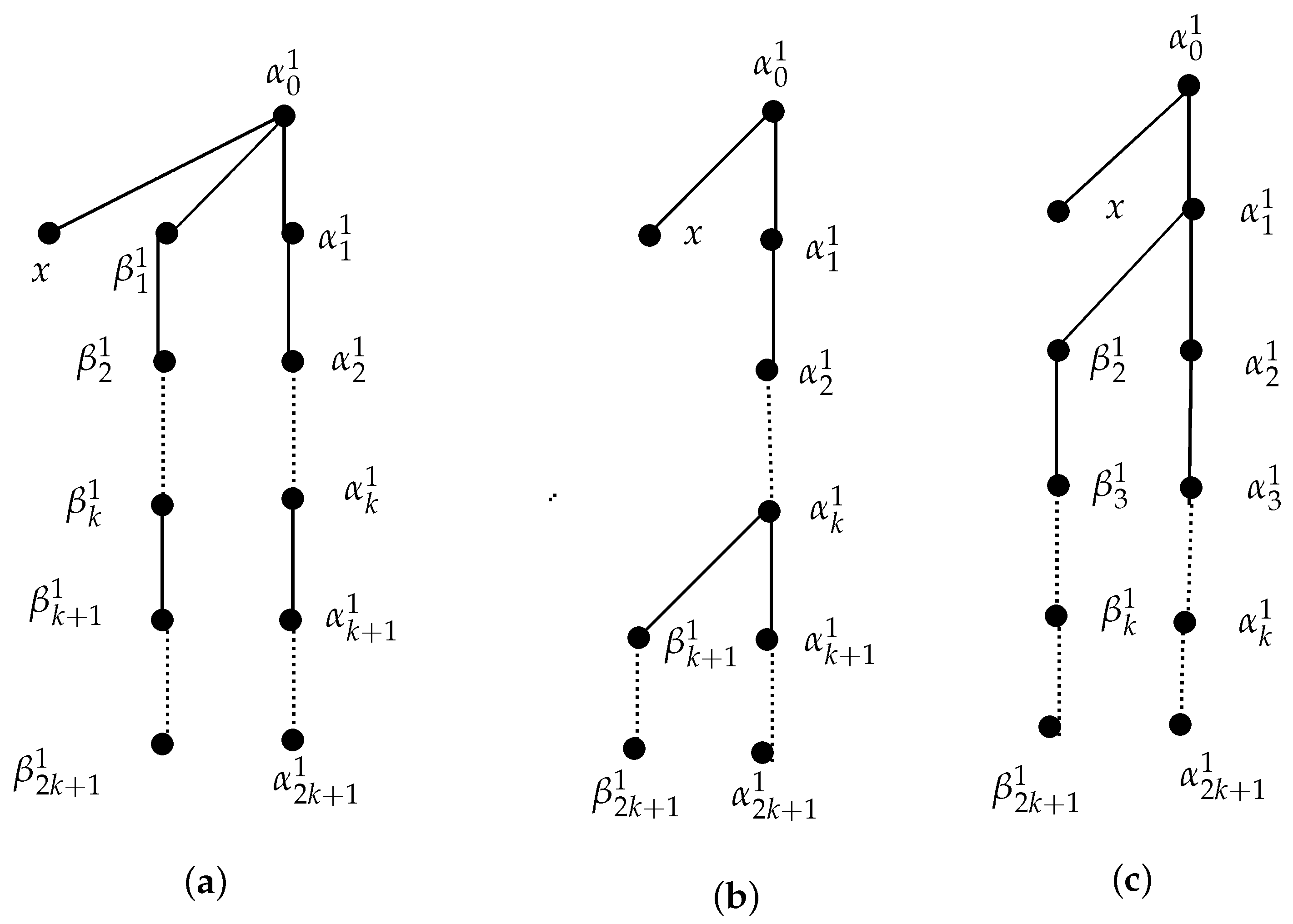
In that case, if the distinct part of the alternative path (${\alpha }_0^1\to {\alpha }_1^1\to \dots \to {\alpha }_k^1\to {\beta }_{k+1}^1\to {\beta }_{k+2}^1\to \dots \to {\beta }_{2k+1}^1$) starts from $k^{th}$ or a higher level of $T_t\left(1\right)$ (see Figure 5b, here, ${\alpha }_0^1\to {\alpha }_1^1\to \dots \to {\alpha }_k^1$ is the common part of both the alternative path and the main path), then $d({\alpha }_k^1,{\alpha }_0^1)=k$ (along the main path), $d({\alpha }_k^1,{\alpha }_1^1)=k-1$, $d({\alpha }_k^1,x)=k+1$ (as $x\to {\alpha }_0^1\to {\alpha }_1^1\to \dots \to {\alpha }_k^1$); $d({\alpha }_k^1,{\alpha }_{2k+1}^1)=k+1$ (along the main path), and $d({\alpha }_k^1,{\beta }_{2k+1}^1)=k+1$ (along the alternative path). So, $d({\alpha }_k^1,y)\le k+1$, ∀$y\in V$ and $Max\{d(u,v):u\in V-\left\{{\alpha }_k^1\right\},v\in V\}\ge k+1$. Therefore, $radius\left(G\right)=k+1$ and ${\alpha }_k$ is a central vertex of the trapezoid graph G. Similarly, some other leaf nodes at $k^{th}$ level of $T_t\left(1\right)$ may be central node of G. So, the center of G lies in $P_k^1$.

Figure 5. Parts of BFS trees.

Again, let the distinct part of the alternative path (${\alpha }_0^1\to {\alpha }_1^1\to {\beta }_2^1\to {\beta }_3^1\to \dots \to {\beta }_{2k+1}^1$) starting from the first level to the ${(k-1)}^{th}$ level of $T_t\left(1\right)$ (see Figure 5c, here, the alternative path and the main path may have a common part above the level $k-1$). Now, if $({\alpha }_i^1,{\beta }_{i+1}^1)\notin E$ and $({\beta }_i^1,{\alpha }_{i+1}^1)\notin E$$\forall i=2, 3,\dots , 2k$, then $d({\alpha }_k^1,{\alpha }_0^1)=k$; $d({\alpha }_k^1,{\alpha }_1^1)=k-1$; $d({\alpha }_k^1,x)=k+1$; $d({\alpha }_k^1,{\alpha }_{2k+1}^1)=k+1$ and $d({\alpha }_k^1,{\beta }_{2k+1}^1)=k+2$ (as ${\alpha }_k^1\to {\beta }_k^1\to {\beta }_{k+1}^1\to \dots \to {\beta }_{2k+1}^1$). So, $d({\alpha }_k^1,y)\le k+2$ for all $y\in V$. Similarly, $d({\beta }_k^1,y)\le k+2$, for all $y\in V$. Also, $d({\alpha }_{k+1}^1,y)\le k+2$ and $d({\beta }_{k+1}^1,y)\le k+2$, ∀ $y\in V$. So, ${\alpha }_k^1,{\alpha }_{k+1}^1,{\beta }_k^1,$ and ${\beta }_{k+1}^1$ are central vertices of G and $radius\left(G\right)=k+2$.

Again, if $({\alpha }_{k-1}^1,{\beta }_k^1)\in E$, $({\beta }_k^1,{\alpha }_{k-1}^1)\in E$, or both, then ${\alpha }_{k-1}^1$, ${\beta }_{k-1}^1$, or both may be central vertices and $radius\left(G\right)=k+1$.

Now, if $({\alpha }_i^1,{\beta }_{i+1}^1)\in E$, (${\beta }_i^1,{\alpha }_{i+1}^1)\in E$, or both, for $i=2, 3,\dots , 2k$, then $d({\alpha }_k^1,y)\le k+1$∀$y\in V$ and $d({\beta }_k^1,y)\le k+1$ ∀$y\in V$. So, $radius\left(G\right)=k+1$ and ${\alpha }_k^1$, ${\beta }_k^1$ will be two central vertices. So, in case 1, $radius\left(G\right)=k+1$ or $radius\left(G\right)=k+2$ and the center lies in ($P=P_{k-1}^1\cup P_k^1\cup P_{k+1}^1$).

Case 2: 

If both ${\alpha }_1^1$ and ${\beta }_1^1$ exist (see Figure 5a, here, the alternative path and the main path are distinct, except the root), then $(x,{\alpha }_1^1)\notin E$ and $(x,{\beta }_1^1)\notin E$, $(x,{\alpha }_2^1)\notin E$ and $({\beta }_i^1,{\alpha }_{i+1}^1)\notin E$ for $i=1,2,\dots ,2k$, ∀$x\in Q_1^1$.

Now, $d({\beta }_{k+1}^1,{\alpha }_0^1)=k+1$ (along the alternative path); $d({\beta }_{k+1}^1,{\alpha }_1^1)=k+1$; $d({\beta }_{k+1}^1,x)=k+1$ (as $x\to {\beta }_1^1\to {\beta }_2^1\to \dots \to {\beta }_{k+1}^1$); $d({\beta }_{k+1}^1,{\beta }_{2k+1}^1)=k$ and $d({\beta }_{k+1}^1,{\alpha }_{2k+1}^1)=k+1$ (as ${\beta }_{k+1}^1\to {\alpha }_{k+1}^1\to {\alpha }_{k+2}^1\to \dots \to {\alpha }_{2k+1}^1$). So, $d({\beta }_{k+1}^1,y)\le k+1$, $\forall y\in V$ and $Max\{d(u,v):u\in V-\left\{{\beta }_{k+1}^1\right\},v\in V\}\ge k+1$. Therefore, $radius\left(G\right)=k+1$ and ${\beta }_{k+1}^1$ is a central vertex of the trapezoid graph G. Similarly, we can show that some other vertices of $P_{k+1}^1$ or $P_k^1$ may be central vertices. So, the center lies in ($P_k^1\cup P_{k+1}^1$).

Hence, $radius\left(G\right)=k+1$ or $radius\left(G\right)=k+2$, and $center\left(G\right)$ lies in $P=(P_{k-1}^1\cup P_k^1\cup P_{k+1}^1)$.

From the above result, we can conclude the following.

Corollary 4. 

If $radius\left(G\right)=k+1$ and $diameter\left(G\right)=2k+2$, then $2\times radius\left(G\right)-diameter\left(G\right)=0$, else if $radius\left(G\right)=k+2$ and $diameter\left(G\right)=2k+2$, then $2\times radius\left(G\right)-diameter\left(G\right)=2$.

From the Corollaries 1–4, we can conclude the following.

Corollary 5. 

For any trapezoid graph G, $2\times radius\left(G\right)-diameter\left(G\right)=k,$$k=0, 1, 2$.

From the previous three results, we have reached the following statement.

Corollary 6. 

$radius\left(G\right)=min\left\{eccentricity\right(x):x\in P\}$.

Proof. 

It is straightforward as $center\left(G\right)\in P$.   □

Note 3. 

The results of Lemmas 6–9 are also true for the BFS trees $T_t\left(n\right),T_t\left(a\right),$ and $T_t\left(b\right)$.

4. Computation of Central Vertices and Radius

Here, we find out the $radius\left(G\right)$ and central vertices of the trapezoid graph G. To achieve this, we compute the set P, where

$$P=\left\{\begin{array}{c}{P}_{k-1}^1\cup P_k^1\cup P_{k+1}^1,\mathrm{if}\mathrm{one\; of} h_1,h_n,h_a, \mathrm{and} h_b \mathrm{is} \mathrm{even}, \mathrm{say} h_1=2k;\hfill \\ diameter\left(G\right)=2k+1,\hfill \\ \\ P_{k-1}^1\cup P_k^1\cup P_{k+1}^1,\mathrm{if}\mathrm{one\; of} h_1,h_n,h_a, \mathrm{and}{h}_b \mathrm{is} \mathrm{even},\hfill \\ \mathrm{say} h_1=2k;diameter\left(G\right)=2k,\hfill \\ \\ P_k^1\cup P_{k+1}^1,\mathrm{if}\mathrm{if\; one\; of} h_1,h_n,h_a, \mathrm{and}{h}_b \mathrm{is} \mathrm{odd}, \mathrm{say},\hfill \\ h_1=2k+1\mathrm{and}diameter\left(G\right)=2k+1,\hfill \\ \\ P_{k-1}^1\cup P_k^1\cup P_{k+1}^1,\mathrm{if}\mathrm{if\; one\; of}{h}_1,h_n,h_a, \mathrm{and} h_b \mathrm{is\; odd}, \mathrm{say},\hfill \\ h_1=2k+1\mathrm{and}diameter\left(G\right)=2k+2,\hfill \\ \end{array}\right.$$

and the vertices of P are arranged in order (descending or ascending).

Let $P=\{x_1,x_2,\dots ,x_{k-1},x_k\}$, $1\le k\le n$. Now, we find a set A where the member of A is the common adjacent trapezoid of $t_1$ and $t_a$ except the trapezoid(s) corresponding to the internal nodes at level 1 of $T_t\left(1\right)$ and $T_t\left(a\right)$. Then, we find

• $q_x=min\{q_i:$ where $q_i$ is the top-right vertex of the trapezoid belonging to the set $A\}$ and
• $s_y=min\{s_i:$ where $s_i$ is the bottom-right vertex of the trapezoid belonging to the set $A\}$.

Again, we find another set B whose members are the common adjacent trapezoid of $t_n$ and $t_b$ except the trapezoid(s) corresponding to the internal nodes at level 1 of $T_t\left(n\right)$ and $T_t\left(b\right)$. Then, we find

• $p_z=$ max{$p_i:$ where $p_i$ is the top-left vertex of the trapezoid belongs to the set B} and
• $r_t=$ max{$r_i:$ where $r_i$ is the bottom-left vertex of the trapezoid belongs to the set B}.

Let us consider $S=\{x,y,z,t\}\subseteq V$, corresponding to $q_x$, $s_y$, $p_z$, $r_t$. Obviously, some or all among $\{1,a,x,y,n,b,z,t\}$ will be the farthest vertices from the members of P. Now, If S is a non-empty set, then we construct the BFS trees $T_t\left(z\right)$, $T_t\left(y\right)$, $T_t\left(x\right),$ and $T_t\left(t\right)$ with $z,y,x,$ and t as roots. Now, we find the distance of the vertices of P from $1,a,x,y$, if they exist, in Table 1 and from $n,b,z,t$, if they exist, in Table 2 with the help of $T_t\left(1\right),T_t\left(a\right),T_t\left(n\right)$, $T_t\left(b\right)$, $T_t\left(x\right),T_t\left(y\right),T_t\left(z\right),$ and $T_t\left(t\right)$.

Table 1. Distance of the vertices of P from $\mathrm{1},a,x,y$.

${\mathit{x}}_{\mathit{i}}$	${\mathit{d}}_{\mathrm{1},\mathit{i}}=\mathit{d}(\mathrm{1},{\mathit{x}}_{\mathit{i}})$	${\mathit{d}}_{\mathit{a},\mathit{i}}=\mathit{d}(\mathit{a},{\mathit{x}}_{\mathit{i}})$	${\mathit{d}}_{\mathit{x},\mathit{i}}=\mathit{d}(\mathit{x},{\mathit{x}}_{\mathit{i}})$	${\mathit{d}}_{\mathit{y},\mathit{i}}=\mathit{d}(\mathit{y},{\mathit{x}}_{\mathit{i}})$	${\mathit{L}}_{\mathit{m}\mathit{a}\mathit{x}}=\mathit{m}\mathit{a}\mathit{x}\{{\mathit{d}}_{\mathrm{1},\mathit{i}},{\mathit{d}}_{\mathit{a},\mathit{i}},{\mathit{d}}_{\mathit{x},\mathit{i}},{\mathit{d}}_{\mathit{y},\mathit{i}}\}$
$x_1$	$d_{1,1}=d(1,x_1)$	$d_{a,1}=d(a,x_1)$	$d_{x,1}=d(x,x_1)$	$d_{y,1}=d(y,x_1)$	$d_{l,1}$ (say)
$x_2$	$d_{1,2}=d(1,x_2)$	$d_{a,2}=d(a,x_2)$	$d_{x,2}=d(x,x_2)$	$d_{y,2}=d(y,x_2)$	$d_{l,2}$ (say)
…	…	…	…	…	…
$x_k$	$d_{1,k}=d(1,x_k)$	$d_{a,k}=d(a,x_k)$	$d_{x,k}=d(x,x_k)$	$d_{y,k}=d(y,x_k)$	$d_{l,k}$ (say)

Table 2. Distance of the vertices of P from $n,b,z,t$.

${\mathit{x}}_{\mathit{i}}$	${\mathit{d}}_{\mathit{n},\mathit{i}}=\mathit{d}(\mathit{n},{\mathit{x}}_{\mathit{i}})$	${\mathit{d}}_{\mathit{b},\mathit{i}}=\mathit{d}(\mathit{b},{\mathit{x}}_{\mathit{i}})$	${\mathit{d}}_{\mathit{z},\mathit{i}}=\mathit{d}(\mathit{z},{\mathit{x}}_{\mathit{i}})$	${\mathit{d}}_{\mathit{t},\mathit{i}}=\mathit{d}(\mathit{t},{\mathit{x}}_{\mathit{i}})$	${\mathit{R}}_{\mathit{m}\mathit{a}\mathit{x}}=\mathit{m}\mathit{a}\mathit{x}\{{\mathit{d}}_{\mathit{n},\mathit{i}},{\mathit{d}}_{\mathit{b},\mathit{i}},{\mathit{d}}_{\mathit{z},\mathit{i}},{\mathit{d}}_{\mathit{t},\mathit{i}}\}$
$x_1$	$d_{n,1}=d(n,x_1)$	$d_{b,1}=d(b,x_1)$	$d_{z,1}=d(z,x_1)$	$d_{t,1}=d(t,x_1)$	$d_{r,1}$ (say)
$x_2$	$d_{n,2}=d(n,x_2)$	$d_{b,2}=d(b,x_2)$	$d_{z,2}=d(z,x_2)$	$d_{t,2}=d(t,x_2)$	$d_{r,2}$ (say)
…	…	…	…	…	…
$x_k$	$d_{n,k}=d(n,x_k)$	$d_{b,k}=d(b,x_k)$	$d_{z,k}=d(z,x_k)$	$d_{t,k}=d(t,x_k)$	$d_{r,k}$ (say)

In Table 3, we compare the corresponding values of $L_{max}$ (in Table 1) and $R_{max}$ (in Table 2) and find $max\{L_{max},R_{max}\}$.

Table 3. Comparison of $L_{max}$ and $R_{max}$.

${\mathit{x}}_{\mathit{i}}$	${\mathit{L}}_{\mathit{m}\mathit{a}\mathit{x}}$	${\mathit{R}}_{\mathit{m}\mathit{a}\mathit{x}}$	$\mathit{m}\mathit{a}\mathit{x}\{{\mathit{L}}_{\mathit{m}\mathit{a}\mathit{x}},{\mathit{R}}_{\mathit{m}\mathit{a}\mathit{x}}\}$
$x_1$	$d_{l,1}$	$d_{r,1}$	$e_1$ (say)
$x_2$	$d_{l,2}$	$d_{r,2}$	$e_2$ (say)
…	…	…	…
$x_k$	$d_{l,k}$	$d_{r,k}$	$e_k$ (say)

So, $e_i=eccentricity\left(x_i\right)$ as $e_i$ is the longest shortest distance of $x_i$ from the farthest vertices of G. Now, we find $e_{min}$ = min{$e_i:i=1, 2,\dots ,k \}$. After then, we find the member of P, say $x_j,1\le j\le k$, corresponding to $e_{min}$, in Table 3. As $center\left(G\right)\in P$, therefore, the smallest value of the eccentricity of the vertices of P must be equal to $radius\left(G\right)$, that is $radius\left(G\right)=e_{min}$, by Corollary 1. Now, we find the $e_i$s at the fourth column of Table 3, which are equal to $e_{min}$ and the $x_i$s corresponding to the $e_i$s are the central vertices G.

4.1. Algorithm and Its Complexity

Here, we propose an algorithm to determine the $diameter\left(G\right)$, $radius\left(G\right),$ and central node(s) of trapezoid graphs based on the results presented in Section 3 and Section 4.

Using Algorithm 1, we obtain $diameter\left(G\right)=5$, $radius\left(G\right)=3,$ and $center\left(G\right)=\{4,8,9,10,11\}$ for the trapezoid graph of Figure 2.

Algorithm 1: Algorithm DIA-RAD-CEN-TRA.

Input: Trapezoid representation $p_i,q_i,r_i,s_i$ of a trapezoid graph G, for $i=1:1:n$. Output: $diameter\left(G\right)$, $radius\left(G\right),$ and central vertices of G. Step 1: Make 4 BFS trees $T_t\left(1\right)$, $T_t\left(n\right)$, $T_t\left(a\right),$ and $T_t\left(b\right)$. Step 2: Obtain the heights $h_1,h_n,h_a,$ and $h_b$ of $T_t\left(1\right)$, $T_t\left(n\right)$, $T_t\left(a\right),$ and $T_t\left(b\right)$, respectively. Step 3: Mark the main paths and alternative-paths of $T_t\left(1\right)$, $T_t\left(n\right)$, $T_t\left(a\right),$ and $T_t\left(b\right)$. Step 4: Find the sets $P_i^1,P_i^a,P_i^n,P_i^b$ for $i=1,2,\dots ,max\{h_1,h_a,h_n,h_b\}$. Step 5: If$h_1=h_n=h_a=h_b=h\left(say\right)$ and there exist at least two nodes $x,y$ such that $x\in (Q_1^1\cap Q_1^a),y\in (Q_1^n\cap Q_1^b)$ and $(x,z)\notin E$, for all $z\in P_2^1\cup P_2^a\cup \{{\alpha }_1^1,{\beta }_1^1,{\alpha }_1^a,{\beta }_1^a\}$ and $(y,t)\notin E$, for all $t\in P_2^n\cup P_2^b\cup \{{\alpha }_1^n,{\beta }_1^n,{\alpha }_1^b,{\beta }_1^b\},$ then $diameter\left(G\right)=h+1$ (by Lemma 4) Else $diameter\left(G\right)=max\{h_1,h_n,h_a,h_b\}$ (Lemma 4). End if Step 6: If one of $h_1,h_n,h_a,$ and $h_b$ is even, say $h_1=2k$ and $diameter\left(G\right)=2k+1,$ then $radius\left(G\right)=k+1$ and set $P=P_{k-1}^1\cup P_k^1\cup P_{k+1}^1$ (Lemma 6). Else if one of $h_1,h_n,h_a,$ and $h_b$ is even, say $h_1=2k$ and $diameter\left(G\right)=2k,$ then $radius\left(G\right)=k$ or $radius\left(G\right)=k+1$ and set $P=P_{k-1}^1\cup P_k^1\cup P_{k+1}^1$ (Lemma 7). Else if one of $h_1,h_n,h_a,$ and $h_b$ are odd, say $h_1=2k+1$ and $diameter\left(G\right)=2k+1$, then $radius\left(G\right)=k+1$ and set $P=P_k^1\cup P_{k+1}^1$ (Lemma 8). Else if one of $h_1,h_n,h_a,$ and $h_b$ are odd, say $h_1=2k+1$ and $diameter\left(G\right)=2k+2$, then $radius\left(G\right)=k+1$ or $radius\left(G\right)=k+2$ and set $P=P_{k-1}^1\cup P_k^1\cup P_{k+1}^1$ (by Lemma 9). Step 7: Arrange the vertices of P in ascending order, say $P=\{x_1,x_2,\dots ,x_{k-1},x_k\}$. Step 8: Step 8.1: Find set A where the members of A are the common adjacent trapezoid of $t_1$ and $t_a$ except the trapezoid(s) corresponding to the internal nodes at level 1 of $T_t\left(1\right)$ and $T_t\left(a\right)$. Step 8.2: Find $q_x=$ min{$q_i:$ where $q_i$ is the top-right vertex of the trapezoid belonging to the set A}. Step 8.3: Find $s_y=$ min{$s_i:$ where $s_i$ is the bottom-right vertex of the trapezoid belonging to the set A}. Step 8.4: Find another set B where the members of B are the common adjacent trapezoid of $t_n$ and $t_b$ except the trapezoid(s) corresponding to the internal nodes at level 1 of $T_t\left(n\right)$ and $T_t\left(b\right)$. Step 8.5: Find $p_z=$ max{$p_i:$ where $p_i$ is the top-left vertex of the trapezoid belonging to the set B}. Step 8.6: Find $r_t=$ max{$r_i:$ where $r_i$ is the bottom-left vertex of the trapezoid belonging to the set B}. Step 9: Compute the set $S=\{x,y,z,t\}$ corresponding to $q_x$, $s_y$, $p_z$, $r_t$. Step 10: If S is a non-empty set, then we construct the BFS trees $T_t\left(z\right),T_t\left(y\right),T_t\left(x\right),$ and $T_t\left(t\right)$ with $z,y,x,$ and t, if they exist, as roots, respectively. Else go to Step 11 End if Step 11: Compute the distance of the vertices of P from $S_1=\{1,a,x,y\}$ (if they exist) and $S_2=\{n,b,z,t\}$ (if they exist), using the Table 1 and Table 2, respectively. Also, find $L_{max}$ and $R_{max}$ using Table 1 and Table 2, respectively. Step 12: Compare the entries in the columns $L_{max}$ (in Table 1) and $R_{max}$ (in Table 2), and find the maximum value for each row using Table 3. Step 13: Find $e_{min}$ where $e_{min}=$ min{$e_i:i=1,2,\dots ,k\}$ and find $center\left(G\right)=\{x_i:x_i(\in P)$ corresponding to $e_i$s (in Table 3), where $e_i=e_{min}\}$. Step 14: Set $radius\left(G\right)=e_{min}$. End if End DIA-RAD-CEN-TRA.

4.2. Explanatory Example

To explain the total compilation process of Algorithm 1, we consider the T-diagram (displayed in Figure 1) of the trapezoid graph of Figure 2. Here, $a=2,n=15,$ and $b=13$. At first (in Step 1), we make four BFS trees $T_t\left(1\right)$, $T_t\left(15\right)$, $T_t\left(2\right),$ and $T_t\left(13\right)$ (shown in Figure 3 and Figure 6). In Step 2, we find the height of $h_1,h_n=h_{15},h_a=h_2,$ and $h_b=h_{13}$ of $T_t\left(1\right)$, $T_t\left(15\right)$, $T_t\left(2\right),$ and $T_t\left(13\right)$, respectively. Here, $h_1=h_{15}=h_2=h_{13}=5$. As there are no node points $x,y$ such that $x\in (Q_1^1\cup Q_1^2)$, $y\in (Q_1^{15}\cup Q^1{3}_1)$ and x is only adjacent with 1, 2, or both and y is only adjacent with 15, 13, or both, therefore, $diameter\left(G\right)=5$(in Step 5). As $h_1=h_{15}=h_2=h_{13}=5=2\times 2+1$ (odd and, here, $k=2$) and $radius\left(G\right)=5$, so $radius\left(G\right)=3$ and $P=P_k^1\cup P_{k+1}^1=P_2^1\cup P_3^1=\{8,6,4,9,10,11\}$ (in Step 6). In Step 7, we arrange the vertices of P in ascending order, so $P=\{4,6,8,9,10,11\}$. In Step 8.1, we are to find the set A where the members of A are the common vertices of $T_t\left(1\right)$ and $T_t\left(2\right)$ at level 1 except the internal nodes. Hence, $A=\varnothing$ and $q_x$ and $s_y$ (in Step 8.2 and Step 8.3) do not exist. In Step 8.4, we are to find the set B whose members are the common vertices of $T_t\left(15\right)$ and $T_t\left(13\right)$ at level 1 except the internal nodes, i.e., $B=\varnothing$. Hence, $p_z$ and $r_t$ (in Step 8.5 and Step 8.6) do not exist. Therefore, $S=\varnothing$ and we go to Step 11. In Step 11, we compute the distance of the vertices of $P=\{4,6,8,9,10,11\}$ from $S_1=\{1,2\}$ in Table 4 (with the help of $T_t\left(1\right),T_t\left(2\right)$) and $S_2=\{15,13\}$ in Table 5 (with the help of $T_t\left(15\right),T_t\left(13\right)$) as follows.

Figure 6. BFS trees $T_t\left(2\right)$ and $T_t\left(13\right)$ of G shown in Figure 2.

Table 4. Distance of the vertices of P from 1, 2.

${\mathit{x}}_{\mathit{i}}$	$\mathit{d}(\mathrm{1},{\mathit{x}}_{\mathit{i}})$	$\mathit{d}(\mathrm{2},{\mathit{x}}_{\mathit{i}})$	${\mathit{L}}_{\mathit{m}\mathit{a}\mathit{x}}=\mathit{m}\mathit{a}\mathit{x}\{{\mathit{d}}_{\mathrm{1},\mathit{i}},{\mathit{d}}_{\mathrm{2},\mathit{i}}\}$
4	$d_{1,1}=2$	$d_{2,1}=2$	$d_{l,1}$ = 2
6	$d_{1,2}=2$	$d_{2,2}=2$	$d_{l,2}$ = 2
8	$d_{1,3}=2$	$d_{2,3}=2$	$d_{l,3}$ = 2
9	$d_{1,4}=3$	$d_{2,4}=3$	$d_{l,4}$ = 3
10	$d_{1,5}=3$	$d_{2,5}=3$	$d_{l,5}$ = 3
11	$d_{1,6}=3$	$d_{2,6}=3$	$d_{l,6}$ = 3

Table 5. Distance of the vertices of P from 15, 13.

${\mathit{x}}_{\mathit{i}}$	$\mathit{d}(\mathrm{15},{\mathit{x}}_{\mathit{i}})$	$\mathit{d}(\mathrm{13},{\mathit{x}}_{\mathit{i}})$	${\mathit{R}}_{\mathit{m}\mathit{a}\mathit{x}}=\mathit{m}\mathit{a}\mathit{x}\{{\mathit{d}}_{15,\mathit{i}},{\mathit{d}}_{13,\mathit{i}}\}$
4	$d_{15,1}=3$	$d_{13,1}=3$	$d_{r,1}$ = 3
6	$d_{15,2}=4$	$d_{13,2}=4$	$d_{r,2}$ = 4
8	$d_{15,3}=3$	$d_{13,3}=3$	$d_{r,3}$ = 3
9	$d_{15,4}=3$	$d_{13,4}=2$	$d_{r,4}$ = 3
10	$d_{15,5}=2$	$d_{13,5}=2$	$d_{r,5}$ = 2
11	$d_{15,6}=2$	$d_{13,6}=3$	$d_{r,6}$ = 3

Now, we compare the entries in the columns $L_{max}$ (in Table 4) and $R_{max}$ (in Table 5), and find the maximum value for each row using the following table at Step 12.

At Step 13, we use the Table 6 to find $e_{min}=min\{3,4,3,3,3,3\}=3$ and $center\left(G\right)=\{x_i:x_i(\in P)$ corresponding to $e_i$s (in Table 6), where $e_i=e_{min}\}=\{4,8,9,10,11\}$. In the last step, we set $radius\left(G\right)=3$. Therefore, the main output of our proposed algorithm is $diameter\left(G\right)=5$, $radius\left(G\right)=3$, and $center\left(G\right)=\{4,8,9,10,11\}$.

Table 6. Comparison table.

${\mathit{x}}_{\mathit{i}}$	${\mathit{L}}_{\mathit{m}\mathit{a}\mathit{x}}$	${\mathit{R}}_{\mathit{m}\mathit{a}\mathit{x}}$	$\mathit{m}\mathit{a}\mathit{x}=\mathit{m}\mathit{a}\mathit{x}\{{\mathit{L}}_{\mathit{m}\mathit{a}\mathit{x}},{\mathit{R}}_{\mathit{m}\mathit{a}\mathit{x}}\}$
4	2	3	$e_1$ = 3
6	2	4	$e_2$ = 4
8	2	3	$e_3$ = 3
9	3	3	$e_4$ = 3
10	3	2	$e_5$ = 3
11	3	3	$e_6$= 3

Theorem 1. 

The $diameter\left(G\right)$, $radius\left(G\right)$ and center of the trapezoid graph G can be determined within $O\left(n\right)$ time, where n represents the cardinality of $V\left(G\right)$.

Proof. 

In Step 1, the BFS trees $T_t\left(1\right)$, $T_t\left(a\right)$, $T_t\left(n\right),$ and $T_t\left(b\right)$ can be made within $O\left(4n\right)\approx O\left(n\right)$ time. The heights $h_1,h_a,h_b,$ and $h_n$ in the Step 2 can be found in constant time. At Step 3, main paths and alternative paths of $T_t\left(1\right)$, $T_t\left(n\right)$, $T_t\left(a\right),$ and $T_t\left(b\right)$ can be identified in $O\left(n\right)$ time. Step 4 needs $O\left(n\right)$ time to compute the sets $P_i^1,P_i^a,P_i^n,P_i^b$ for $i=1, 2,\dots ,max\{h_1,h_a,h_n,h_b\}$. In Step 5, $diameter\left(G\right)$ can be determined in $O\left(n\right)$ time. We can compute the set P, at Step 6, within $O\left(n\right)$ time. Also, we can arrange the members of P in ascending order, at Step 7, in just $O\left(n\right)$ time. The determination process of the sets A and B and corner points $q_x$, $s_y$, $p_z$, and $r_t$ just take $O\left(n\right)$ time, in Step 8. Also, Step 9 takes constant time. In Step 10, BFS trees $T_t\left(z\right)$, $T_t\left(y\right)$, $T_t\left(x\right),$ and $T_t\left(t\right)$ can be made within $4O\left(n\right),$ which is equivalent to $O\left(n\right)$ time. At Step 11, we can find the distance of the vertices of P from $S_1=\{1,a,x,y\}$ within $O\left(4n\right)\approx O\left(n\right)$ time and, also, the distance of the vertices of P from $S_2=\{n,b,z,t\}$ in $O\left(4n\right)\approx O\left(n\right)$ time. Further, at Step 12, we can evaluate $e_i$s in constant time. Again, at Step 13, anyone can determine $e_{min}$ within $O\left(n\right)$ time and $center\left(G\right)$ in $O\left(n\right)$ time. The execution time of Step 14 is constant. Hence, the overall run time of the Algorithm 1 is $O\left(n\right)$. □

5. Real Application

Here, we present a real application of the center of trapezoid graphs. We consider a real center location problem and present its algorithmic solution with the help of our studied results.

Step-by-step representation of center location problem using a trapezoid graph and its algorithmic solution

Step 1: Proposed problem set up

Consider a center location problem where we have a finite set of blocks (subdivisions of a district), $B=B_1 ,B_2,\dots , B_n$, in a district. We aim to find a central location to establish a private hospital that serves all the people in the district and minimizes the maximum distance from the hospital to any block. To achieve this, we first identify a well-connected location (near a national highway (NH) or state highway (SH)) within each block for a potential hospital site, ensuring that no two sites have the same latitude and longitude. Let these locations be $P_1 ,P_2,\dots , P_n$, where $P_i\dots B_i$ for $i=1, 2,\dots , n$. Let $l_i$ and $L_i$ represent the latitude and longitude of the candidate hospital at $P_i$. We assume each hospital will provide free ambulance services within a certain distance (say 20 km) radius, which we consider the hospital’s range. Our main objective is to find a “center” location that minimizes the farthest distance from it to any point $P_i$ for $i=1, 2,\dots , n$.

Step 2: Represent each location for candidate hospital as an interval on two parallel lines

Draw two parallel horizontal lines, Line 1 and Line 2. Two horizontal parallel lines represent the range of each hospital’s free ambulance service. For each point $P_i$, define an interval $[p_i,q_i]$ taking $L_i$ as center and place it on Line 1 and another interval $[r_i,s_i]$ taking $L_i$ as the center and place it on Line 2, where, $[p_i,q_i]$ represents the length of the national or state highway, which is the maximum, in block $B_i$; $[r_i,s_i]$ represents the average distance of local roads from $P_i$ to all the areas in block $B_i$.

Step 3: Construct trapezoids based on intervals

For each point $P_i$, construct a trapezoid by connecting the endpoints of its intervals on Line 1 and Line 2. Each trapezoid represents the potential area of influence for a candidate hospital. For instance, for point $P_1$, connect point $p_1$ on Line 1 to point $r_1$ on Line 2, and connect $q_1$ on Line 1 to $s_1$ on Line 2 to form a trapezoid.

Step 4: Create a trapezoid graph

Vertices: Each trapezoid represents a vertex/node in the trapezoid graph.

Edges: Draw an edge between two nodes if their corresponding trapezoids intersect (overlap). This indicates that there is a potential overlap in the service area between the corresponding locations. For example, suppose the service area of $P_1$ covers the whole area of block $B_1$ and partial areas of blocks $B_2$ and $B_3$ and that of $P_2$ covers the whole area of block $B_2$ and partial areas of blocks $B_1$ and $B_3$. So, there is service overlapping between these hospitals. So, there will be an edge between the vertices representing these trapezoids corresponding to the locations $P_1$ and $P_2$.

To illustrate the above steps graphically, we consider a district that has four blocks $B_1$, $B_2$, $B_3$, and $B_4$, and its five parameters of candidate hospitals are given in Table 7. The graphical representation of our proposed problem is displayed in Figure 7 and Figure 8.

Table 7. Parameters of our proposed problem.

Name of Blocks	Hospital’s Position	Latitude	Longitude	Length of NH/SH	Average Local Route Distance	Free Range of Ambulance
$B_1$	$P_1$	$l_1$	$L_1$	$d_1$	$a_1$	K
$B_2$	$P_2$	$l_2$	$L_2$	$d_2$	$a_2$	K
$B_3$	$P_3$	$l_3$	$L_3$	$d_3$	$a_3$	K
$B_4$	$P_4$	$l_4$	$L_4$	$d_4$	$a_4$	K

Figure 7. Trapezoidal representation of proposed problem.

Figure 8. Trapezoid graph of proposed problem.

Step 5: Identification of the center location in the trapezoid graph

The center location problem is now represented as finding a node in the trapezoid graph that minimizes the greatest graph distance to all other nodes. This node represents the optimal location for the facility.

Now, if we compile our designed Algorithm DIA-RAD-CEN-TRA for the trapezoid graph corresponding to the proposed problem, then we will obtain the central vertices in $O\left(n\right)$ time. Any member of the center of the trapezoid graph is suitable for setting up a private hospital that minimizes the farthest distance from it to other vertices.

6. Conclusions

The center location problem is a crucial problem in graph theory. In this paper, we explore some characteristics of the BFS tree of trapezoid graphs. We also study new properties that relate to the radius, the diameter, and the center of trapezoid graphs. For the trapezoid graph G, we prove that the difference between the $diameter\left(G\right)$ and the height of the BFS trees $T_t\left(1\right),T_t\left(n\right),T_t\left(a\right),$ and $T_t\left(b\right)$ is at most one. We also establish a relationship ($2\times radius\left(G\right)-diameter\left(G\right)=k, k=0, 1, 2$) between $radius\left(G\right)$ and $diameter\left(G\right)$ of trapezoid graphs. This result is slightly better than the result of [38] for $k=0, 1$. We also prove that, to find the radius, the diameter, and the center of trapezoid graphs it is not necessary to find the eccentricity of all vertices. We also design an $O\left(n\right)$ time algorithm to find the radius, the diameter, and the center of trapezoid graphs. We also calculate the time complexity of our proposed algorithm. Besides these, we consider a center location problem for identifying a center location in a district to construct a private hospital that minimizes the farthest distance from the hospital to other places in the district. We present an algorithmic solution of the proposed problem with the help of a trapezoid graph model and using BFS graph traversal technique within $O\left(n\right)$ time. In the future, we have a plan to solve different center location problems using other graph models.

References

- Dagan, I.; Golumbic, M.C.; Pinter, R.Y. Trapezoid graphs and their coloring. Discret. Appl. Math. 1988, 21, 35–46. [Google Scholar] [CrossRef]
- Ma, T.; Spinrad, J.P. An O(n2) algorithm for 2-chain problem on certain classes of perfect graphs. In Proceedings of the 2nd ACM-SIAM Symposium on Discrete Algorithms, San Francisco, CA, USA, 28–30 January 1991. [Google Scholar]
- Corneil, D.G.; Kamula, P.A. Extension of permutation and interval graphs. Congr. Numer. 1987, 58, 267–276. [Google Scholar]
- Golumbic, M.C. Algorithmic Graph Theory and Perfect Graphs; Elsevier B.V.: Amsterdam, The Netherlands, 2004; Volume 57. [Google Scholar]
- Liang, Y.D. Domination in trapezoid graphs. Inf. Process. Lett. 1994, 52, 309–315. [Google Scholar] [CrossRef]
- Pramanik, T.; Mondal, S.; Pal, M. The Diameter of an Interval Graph is Twice of its Radius. World Acad. Sci. Technol. Int. J. Math. Comput. Phys. Electr. Comput. Eng. 2011, 5, 1412–1417. [Google Scholar]
- Abbound, A.; Grandoni, F.; Williams, V.V. Subcubic Equivalences Between Graph Centrality Problems, APSP and diameter. In Proceedings of the 26th Annual ACM-SIAM Symposium on Discrete Algorithms, San Diego, CA, USA, 4–6 January 2015; pp. 1681–1697. [Google Scholar]
- Stummer, C.; Doerner, K.; Focke, A.; Heidenberger, K. Determining location and size of medical departments in a hospital network: A multiobjective decision support approach. Health Care Manag. Sci. 2004, 7, 63–71. [Google Scholar] [CrossRef]
- Wu, C.R.; Lin, C.T.; Chen, H.C. Optimal selection of location for Taiwanese hospitals to ensure a competitive advantage by using the analytic hierarchy process and sensitivity analysis. Build. Environ. 2007, 42, 1431–1444. [Google Scholar] [CrossRef]
- Syam, S.S. A multiple server location-allocation model for service system design. Comput. Oper. Res. 2008, 5, 2248–2265. [Google Scholar] [CrossRef]
- Vahidnia, M.H.; Alesheikh, A.A.; Alimohammadi, A. Hospital site selection using fuzzy AHP and its derivatives. J. Environ. Manag. 2009, 90, 3048–3056. [Google Scholar] [CrossRef] [PubMed]
- Shariff, S.S.R.; Moin, N.H.; Omar, M. Location allocation modeling for healthcare facility planning in Malaysia. Comput. Ind. Eng. 2012, 62, 1000–1010. [Google Scholar] [CrossRef]
- Kim, D.G.; Kim, Y.D. A Lagrangian heuristic algorithm for a public healthcare facility location problem. Ann. Oper. Res. 2013, 206, 221–240. [Google Scholar] [CrossRef]
- Shariff, S.S.R.; Moin, N.H.; Omar, M. Planning of public healthcare facility using a location allocation modelling: A case study. In Proceedings of the Statistics and Operational Research International Conference (SORIC 2013), Sarawak, Malaysia, 3–5 December 2013; AIP Publishing LLC: Melville, NY, USA, 2014; Volume 296, pp. 282–296. [Google Scholar] [CrossRef]
- Beheshtifar, S.; Alimoahmmadi, A. A multiobjective optimization approach for location-allocation of clinics. Int. Trans. Oper. Res. 2015, 22, 313–328. [Google Scholar] [CrossRef]
- Elkady, S.K.; Abdelsalam, H.M. A simulation-based optimization approach for healthcare facility location allocation decision. In Proceedings of the Science and Information Conference 2015, London, UK, 28–30 July 2015; pp. 500–505. [Google Scholar]
- Maric, M.; Stanimirovic, Z.; Bozovic, S. Hybrid metaheuristic method for determining locations for long-term health care facilities. Ann. Oper. Res. 2015, 227, 3–23. [Google Scholar] [CrossRef]
- Elkady, S.K.; Abdelsalam, H.M. A modified multi-objective particle swarm optimisation algorithm for healthcare facility planning. Int. J. Bus. Syst. Res. 2016, 10, 1–22. [Google Scholar] [CrossRef]
- Ouyang, R.; Faiz, T.I.; Noor-E-Alam, M. An ILP model for healthcare facility location problem with long term demand. In Proceedings of the 2016 International Conference on Industrial Engineering and Operations Management, Kuala Lumpur, Malaysia, 8–10 March 2016; IEOM Society International: Detroit, MI, USA, 2014; pp. 840–847. [Google Scholar]
- Ye, H.; Kim, H. Locating healthcare facilities using a network-based covering location problem. GeoJournal 2016, 81, 875–890. [Google Scholar] [CrossRef]
- Zhang, W.; Cao, K.; Liu, S.; Huang, B. A multi-objective optimization approach for health-care facility location-allocation problems in highly developed cities such as Hong Kong. Comput. Environ. Urban Syst. 2016, 59, 220–230. [Google Scholar] [CrossRef]
- Behzad, M.; Chartrand, G. Introduction to the Theory of Graphs; Allyn and Bacon: Boston, MA, USA, 1971. [Google Scholar]
- Cheopoi, V. Centers of Triangulated Graphs. Mat. Zametki 1988, 43, 143–151. [Google Scholar] [CrossRef]
- Takes, F.W.; Kosters, W.A. Determining the Diameter of Small World Networks. In proceedings of the In Proceedings of the 20th ACM Conference on Information and Knoledge Management (CIKM 2011), Glasgow, UK, 24–28 October 2011; pp. 1191–1196. [Google Scholar] [CrossRef]
- Farley, A.; Proskurowski, A. Computation of the Center and Diameter of Outerplanar Graphs. Discret. Appl. Math. 1980, 2, 185–191. [Google Scholar] [CrossRef]
- Goldman, A.J. Minimax Location of a Facility in a Network. Transp. Sci. 1972, 6, 407–418. [Google Scholar] [CrossRef]
- Pal, M.; Bhattacharjee, G.P. Optimal Sequential and Parallel Algorithms for Computing the Diameter and the Center of Interval Graph. Int. J. Comput. Math. 1995, 59, 1–13. [Google Scholar] [CrossRef]
- Chepoi, V.D.; Dragan, F. A Linear-time Algorithm for Finding a Central Vertex of a Chordal Graph. Lect. Notes Comput. Sci. 1994, 855, 159–170. [Google Scholar] [CrossRef]
- Lan, Y.F.; Wanga, Y.L.; Suzuki, H. A Linear-time Algorithm for Solving the Center Problem on Weighted Cactus Graphs. Inf. Process. Lett. 1999, 71, 205–212. [Google Scholar] [CrossRef]
- Olariu, S. A Simple Linear Time Algorithm for Computing the Center of an Interval Graph. Int. J. Comput. Math. 1990, 34, 121–128. [Google Scholar] [CrossRef]
- Olariu, S.; Schwing, J.L.; Zhang, J. Optimal Parallel Algorithms for Problems Modelled by a Family of Intervals. IEEE Trans. Parallels Distrib. Syst. 1992, 3, 364–374. [Google Scholar] [CrossRef]
- Saha, A. Computation of Average Distance, Radius and Center of a Circular-Arc Graph in Parallel. J. Phys. Sci. 2006, 10, 178–187. [Google Scholar]
- Borassi, M.; Cresccnzi, P.; Habib, M.; Kosters, W.A.; Marino, A.; Takes, F.W. Fast Diameter and Radius BFS- based Computation in(weakly connected) Real-World Graphs: With an application to the six degrees of separation games. Theory Comput. Sci. 2015, 586, 59–80. [Google Scholar] [CrossRef]
- Abbound, A.; Wang, J.; Williams, V.V. Approximation and Fixed Parameter Sub Quadratic Algorithms for Radius and Diameter in Sparse Graphs. In Proceedings of the 27th Annual ACM-SIAM Symposium on Discrete Algorithms, Arlington, VA, USA, 10–12 January 2016; pp. 377–391. [Google Scholar]
- Laskar, R.; Shier, D. On powers and centers of chordal graphs. Discret. Appl. Math. 1983, 6, 139–147. [Google Scholar] [CrossRef]
- Mahesh, C.P. Distance in Graph Theory and its Application. Int. J. Adv. Eng. Technol. 2011, 3, 147–150. [Google Scholar]
- Nandi, S.; Mondal, S.; Barman, S.C. Computation of diameter, radius and center of permutation graphs. Discret. Math. Algorithms Appl. 2021, 14, 2250039. [Google Scholar] [CrossRef]
- Prisner, E. Radius versus diameter in cocomparability and intersection graphs. Discret. Math. 1997, 163, 109–117. [Google Scholar] [CrossRef]
- Tarjan, R.E. Depth-First Search and Linear Graph Algorithms. SIAM J. Comput. 1972, 1, 146–160. [Google Scholar] [CrossRef]
- Chen, C.C.Y.; Das, S.K. Breadth-First Traversal of Trees and Integer Sorting in Parallel. Inf. Process. Lett. 1992, 41, 39–49. [Google Scholar] [CrossRef]
- Olariu, S. An Optimal Greedy Heuristic to Color Interval Graphs. Inf. Process. Lett. 1991, 37, 21–25. [Google Scholar] [CrossRef]
- Barman, S.; Mondal, S.; Pal, M. An Efficient Algorithm to find Next-to-Shortest Path on Permutation Graphs. J. Appl. Math. Comput. 2009, 31, 369–384. [Google Scholar] [CrossRef]
- Mondal, S.; Pal, M.; Pal, T.K. An optimal algorithm for solving all-pairs shortest paths on trapezoid graphs. Int. J. Comput. Eng. Sci. 2002, 3, 103–116. [Google Scholar] [CrossRef]
- Barman, S.; Mondal, S.; Pal, M. A Linear Time Algorithm to Construct a Tree 4-Spanner on Trapezoid Graphs. Int. J. Comput. Math. 2010, 87, 743–755. [Google Scholar] [CrossRef]
Disclaimer/Publisher’s Note: The statements, opinions and data contained in all publications are solely those of the individual author(s) and contributor(s) and not of MDPI and/or the editor(s). MDPI and/or the editor(s) disclaim responsibility for any injury to people or property resulting from any ideas, methods, instructions or products referred to in the content. |
© 2025 by the authors. Licensee MDPI, Basel, Switzerland. This article is an open access article distributed under the terms and conditions of the Creative Commons Attribution (CC BY) license (https://creativecommons.org/licenses/by/4.0/).