On Error Estimation and Convergence of the Difference Scheme for a Nonlinear Elliptic Equation with an Integral Boundary Condition

Abstract

In this paper, a two-dimensional nonlinear elliptic equation with an integral boundary condition depending on two parameters is investigated. The problem is solved using the finite difference method. The error in the solution is evaluated based on the properties of M-matrices, and herewith the convergence of the difference scheme is proved. The majorant is constructed to estimate the error of the solution of the system of difference equations.

1. Introduction and Problem Statement

In this paper, we consider the boundary value problem for a nonlinear elliptic equation with a nonlocal integral condition that depends on two parameters, $\xi$ and $\gamma$:

$$\begin{array}{cc}\hfill & {\displaystyle \frac{{\partial }^{2}u}{\partial x^2}}+{\displaystyle \frac{{\partial }^{2}u}{\partial y^2}}=f(x,y,u),(x,y)\in \Omega =\{0<x<1,0<y<1\},\hfill \end{array}$$

(1)

$$\begin{array}{cc}\hfill & u(x,0)={\mu }_1\left(x\right),u(x,1)={\mu }_2\left(x\right),u(0,y)={\mu }_3\left(y\right),\hfill \end{array}$$

(2)

$$\begin{array}{cc}\hfill & u(1,y)=\gamma \underset{\xi }{\overset{1}{\int }}u(x,y)dx+{\mu }_4\left(y\right),\hfill \end{array}$$

(3)

where

$$\gamma \ge 0,0\le \xi <1.$$

In recent decades, boundary value problems for differential equations with nonlocal conditions have become a rapidly developing field in the theory of differential equations and numerical analysis. The first two articles on the heat equation with integral boundary conditions [1,2] sparked significant interest among mathematicians, leading to extensive research in this area.

Mathematical models incorporating various types of nonclassical unconventional boundary conditions have been formulated to describe real-world processes and phenomena in fields such as thermoelasticity, population dynamics, inverse problems, control theory, biological processes, chemical diffusion, etc. [1,3,4,5] (see also survey papers [6,7,8]).

Additionally, boundary value problems with nonlocal conditions can be viewed as theoretical generalizations of classical boundary problems. For instance, [9] was written with this intention, anticipating further investigations and applications. Subsequent research by other authors has focused on specific nonlocal conditions and their practical applications.

Various numerical methods have been employed to solve boundary value problems for elliptic equations with nonlocal conditions, with the finite difference method being one of the most commonly used approaches. In [10], a difference scheme of second-order accuracy for an elliptic equation with a Bitsadze–Samarskii-type nonlocal integral condition was theoretically substantiated. The well-possessedness of this difference scheme in Hölder space is proved. A multi-dimensional elliptic equation with integral boundary conditions was examined in [11]. In [12], the Poisson equation in a rectangular domain with integral conditions was solved. It was proven that the corresponding difference scheme converges in the energy norm with a convergence rate of $O\left(h^{s-1}\right)$, $1<s\le 3$, depending on the smoothness of the solution. The author of [13] presents iterative methods for the numerical solution of a class of nonlinear reaction-diffusion equations with nonlocal boundary conditions for both time-dependent and steady-state cases.

The eigenvalue problem, existence, and dynamic behaviour of solutions for linear and semi-linear elliptic and parabolic equations with nonlocal integral boundary conditions are investigated in [13]. A novel approach for solving the elliptic equation with two nonlocal conditions was introduced in [14].

Several papers have addressed high-order accuracy schemes. In [15], a fourth-order difference scheme for the two-dimensional Poisson equation in a rectangular domain with two integral conditions was constructed. The eigenvalue problem for this difference scheme is also considered. A difference scheme of fourth-order accuracy for the Laplace equation with a nonlocal Bitsadze–Samarskii condition was investigated in [16]. Another difference scheme of fourth-order accuracy for the Poisson equation with an integral condition was developed in [17], where it was proven that this scheme can achieve an asymptotic optimal error estimate in the maximum norm using the Fourier transformation.

A separate investigation problem in the finite difference method are the methods of solution in systems of difference equations. The matrices of these systems, which incorporate nonlocal conditions, exhibit two notable properties. First, in all cases except the ones with periodic conditions, the matrix is nonsymmetric. Second, the structure of spectrum of this matrix can change significantly depending on the values of varying parameters or functions in the nonlocal conditions. In recent years, increased attention has been given to two iterative methods: those based on the theory of M-matrices (the principle of regular splitting) [18,19] and ADI methods [20]. In analysing the convergence conditions for these iterative methods, many researchers have studied the structure of spectrum of difference equation systems with nonlocal conditions. As a result, investigations into nonlocal conditions have contributed to the study of eigenvalue problems for nonsymmetric matrices.

The structure of the spectrum of a one-dimensional eigenvalue problem with an integral nonlocal condition in the form (3) was examined in [21], while the structure of spectrum of the corresponding difference eigenvalue problem was analysed in [22,23]. Investigations into spectrum structures with other integral and two-point nonlocal conditions were conducted in [21,22,24,25,26,27,28]. The structure of the spectrum for an ordinary differential equation with nonlocal conditions (3) was investigated in [29].

Although relatively few studies focus on the practical applications of elliptic equations with nonlocal conditions, some notable examples exist. One such application involves the design of electrical contacts controlled by magnetic interaction forces [30], where the nonlinear equation of a surface with prescribed mean curvature serves as the mathematical model. Another example is a boundary value problem for the Vlasov–Poisson equation, which plays a role in designing thermonuclear fusion reactors [5].

Various numerical methods have been applied to solve elliptic equations with nonlocal conditions. The finite element method has been used for different forms of elliptic equations with various nonlocal conditions [31,32,33,34]. In [35], a composite scheme based on the finite element method is presented, with a proof of third-order convergence. In [36,37], the discrete comparison principle for the finite difference and finite elements methods is considered. Other approaches, including the Legendre–Galerkin spectral method and its modifications [38,39] and the radial basis function method [40], have also been employed. A comparative analysis of various numerical methods is provided in [41]. The linear and semi-linear elliptic equations with integral Neumann boundary conditions were investigated in [42,43].

In recent years, interest in new mathematical models has grown. One such model is fractional elliptic equations and their applications [44,45,46]. These studies have been motivated by both emerging practical problems and inside mathematical developments. Additionally, initial research on stochastic differential equations with nonlocal conditions has appeared [47].

In this paper, we consider the boundary value problem (1)–(3) for the nonlinear Poisson Equation (1) with the integral condition (3). Our investigation is based on the theory of M-matrices, with the primary goal of proving the convergence of the difference scheme. Specifically, we aim to determine values of $\gamma >0$ for which the matrix of the difference equation system is an M-matrix. To prove the convergence of the difference scheme in the norm C, we construct a majorant. While our approach follows the standard method of proving convergence, we introduce a new idea: in the standard method, a majorant is typically constructed if the maximum principle is valid for the difference scheme. However, we demonstrate that the maximum principle is not a necessary condition for convergence; instead, it suffices for the matrix of the difference problem to be an M-matrix.

The values of the solution of a two-dimensional problem (1)–(3) in one coordinate direction are connected by an integral nonlocal condition (3). This is the characteristic approach of nonlocal conditions for elliptic equation in two- or multi-dimensional cases [10,11,12].

We have used this approach in our previous studies [18] as well, proving the convergence of iterative methods for both linear and nonlinear elliptic equations with nonlocal conditions. We use our previous results [23,48,49] from the application of M-matrices to the theoretical study of the system of difference equations, showing that the theory of M-matrices could be treated as an extension of the maximum principle in the case where the matrix of the system of difference equations is not diagonally dominant.

The structure of this paper is as follows: In Section 2, we construct the difference problem corresponding to the differential problem (1)–(3). In Section 3 we present some results from M-matrix theory. Section 4 investigates the difference eigenvalue problem. Based on the spectral structure of the difference problem, Section 5 presents a comparison theorem. There, we construct the majorant for the error in the solution. This error is estimated in Section 6. Numerical results illustrating the details of the error estimates are provided in Section 7. Finally, Section 8 presents conclusions and possible generalizations.

2. Difference Problem

Suppose that the differential problem (1)–(3) has a unique, sufficiently smooth solution such that its derivatives up to the fourth order are bounded. Then, we write the following difference problem:

$$\begin{array}{cc}\hfill & {\displaystyle \frac{U_{i-1,j}-2U_{ij}+U_{i+1,j}}{h^2}}+{\displaystyle \frac{U_{i,j-1}-2U_{ij}+U_{i,j+1}}{h^2}}=f(x_i,y_j,U_{ij}),i,j=1,2,\dots ,N-1,\hfill \end{array}$$

(4)

$$\begin{array}{cc}\hfill & U_{i0}={\left({\mu }_1\right)}_i,U_{iN}={\left({\mu }_2\right)}_i,U_{0j}={\left({\mu }_3\right)}_j,i,j=0,1,\dots ,N,\hfill \end{array}$$

(5)

$$\begin{array}{cc}\hfill & U_{Nj}=h\gamma \left({\displaystyle \frac{U_{mj}+U_{Nj}}{2}}+\sum _{i=m+1}^{N-1}{U}_{ij}\right)+{\left({\mu }_4\right)}_j,j=1,2,\dots ,N-1,\hfill \end{array}$$

(6)

where

$$h={\displaystyle \frac{1}{N}},\xi =mh$$

and $N,m$ arenatural numbers.

We denote $u_{ij}$ as the solution of the differential problem (1)–(3) and $U_{ij}$ as the solution of difference problem (4)–(6). For the solution $u_{ij}$ of differential problem (1)–(3), the system of difference equations is as follows:

$$\begin{array}{cc}\hfill & {\displaystyle \frac{u_{i-1,j}-2u_{ij}+u_{i+1,j}}{h^2}}+{\displaystyle \frac{u_{i,j-1}-2u_{ij}+u_{i,j+1}}{h^2}}=f(x_i,y_j,u_{ij})+R_{ij}\left(h\right),i,j=1,2,\dots ,N-1,\hfill \end{array}$$

(7)

$$\begin{array}{cc}\hfill & u_{i0}={\left({\mu }_1\right)}_i,u_{iN}={\left({\mu }_2\right)}_i,u_{0j}={\left({\mu }_3\right)}_j,i=0,1,\dots ,N,j=0,1,\dots ,N,\hfill \end{array}$$

(8)

$$\begin{array}{cc}\hfill & u_{Nj}=h\gamma \left({\displaystyle \frac{u_{mj}+u_{Nj}}{2}}+\sum _{i=m+1}^{N-1}{u}_{ij}\right)+{\left({\mu }_4\right)}_j+R_{Nj}\left(h\right),j=1,2,\dots ,N-1,\hfill \end{array}$$

(9)

where N, m are natural numbers.

The following approximations are correct for approximation errors (under the condition that the solution of the differential problem (1)–(3) is sufficiently smooth):

$$\begin{array}{cc}\hfill & |R_{ij}\left(h\right)|\le {\displaystyle \frac{h^2}{6}}{M}_4,i,j=1,2,\dots ,N-1,\hfill \end{array}$$

(10)

$$\begin{array}{cc}\hfill & |R_{Nj}\left(h\right)|\le {\displaystyle \frac{h^2}{12}}\gamma M_2,j=0,1,\dots ,N-1,\hfill \end{array}$$

(11)

where

$$M_2=max\left(\left|{\displaystyle \frac{{\partial }^{2}u}{\partial x^2}}\right|\right),M_4=max\left(\left|{\displaystyle \frac{{\partial }^{4}u}{\partial x^4}}\right|,\left|{\displaystyle \frac{{\partial }^{4}u}{\partial y^4}}\right|\right).$$

Then, the error could be defined as

$$z_{ij}=u_{ij}-U_{ij}.$$

(12)

From Equations (4)–(6) and Equations (7)–(9), we obtain the following system for the error

$$\begin{array}{cc}\hfill & {\displaystyle \frac{z_{i-1,j}-2z_{ij}+z_{i+1,j}}{h^2}}+{\displaystyle \frac{z_{i,j-1}-2z_{ij}+z_{i,j+1}}{h^2}}={\displaystyle \frac{\partial \tilde{f}}{\partial u}}{z}_{ij}+R_{ij}\left(h\right),i,j=1,2,\dots ,N-1,\hfill \end{array}$$

(13)

$$\begin{array}{cc}\hfill & z_{i0}=z_{iN}=z_{0j}=0,i=0,1,\dots ,N,j=0,1,\dots ,N,\hfill \end{array}$$

(14)

$$\begin{array}{cc}\hfill & z_{Nj}=h\gamma \left({\displaystyle \frac{z_{mj}+z_{Nj}}{2}}+\sum _{i=m+1}^{N-1}{z}_{ij}\right)+R_{Nj}\left(h\right),j=1,2,\dots ,N-1.\hfill \end{array}$$

(15)

From the nonlocal condition (15), we express

$$z_{Nj}=\sum _{i=1}^{N-1}{\alpha }_i{z}_{ij}+\beta R_{Nj}\left(h\right),$$

(16)

where

$${\alpha }_i=\left\{\begin{array}{c}0,i=1,2,\dots ,m-1,\hfill \\ {\displaystyle \frac{h\gamma }{2-h\gamma }},i=m,\hfill \\ {\displaystyle \frac{2h\gamma }{2-h\gamma }},i=m+1,m+2,\dots ,N-1,\hfill \end{array}\right.$$

and

$$\beta ={\displaystyle \frac{2}{2-h\gamma }},m={\displaystyle \frac{\xi }{h}}.$$

We enter $z_{Nj}$ from (16) into Equation (13), where $i=N-1$. Then, we rewrite the system (13)–(15) in another form

$$\begin{array}{cc}\hfill & {\displaystyle \frac{z_{i-1,j}-2z_{ij}+z_{i+1,j}}{h^2}}+{\displaystyle \frac{z_{i,j-1}-2z_{ij}+z_{i,j+1}}{h^2}}={\displaystyle \frac{\partial \tilde{f}}{\partial u}}{z}_{ij}+R_{ij}\left(h\right),i=1,2,...,N-2,j=1,2,...,N-1,\hfill \end{array}$$

(17)

$$\begin{array}{cc}\hfill & {\displaystyle \frac{z_{N-2,j}-2z_{N-1,j}+{\displaystyle \sum _{i=1}^{N-1}}{\alpha }_{ij}{z}_{ij}}{h^2}}+{\displaystyle \frac{z_{N-1,j-1}-2z_{N-1,j}+z_{N-1,j+1}}{h^2}}={\displaystyle \frac{\partial \tilde{f}}{\partial u}}{z}_{Nj}+R_{Nj}\left(h\right),j=1,2,\dots ,N-1,\hfill \end{array}$$

(18)

$$\begin{array}{cc}\hfill & z_{i0}=z_{iN}=z_{0j}=0,i=0,1,\dots ,N,j=0,1,\dots ,N.\hfill \end{array}$$

(19)

Remark 1. 

The system (13)–(15) is equivalent to the system (17)–(19) along with (16). It is important to note that by rearranging the system (13)–(15), we separated the system (17)–(19) without the nonlocal condition. The system (17)–(19), which contains ${(N-1)}^2$ equations and ${(N-1)}^2$ unknowns $z_{ij}$, $i,j=1,2,\dots ,N-1$, can be investigated separately (without nonlocal conditions).

The system (17)–(19) can be presented in matrix form

$$Az+Dz=r\left(h\right).$$

(20)

Here, $r\left(h\right)=\left\{r_{ij}\left(h\right)\right\}$ is vector

$$r_{ij}\left(h\right)=\left\{\begin{array}{c}{R}_{ij}\left(h\right)i=1,2,\dots ,N-1;j=1,2,\dots ,N-1,\hfill \\ R_{N-1,j}+{\displaystyle \frac{\beta }{h^2}}{R}_{N,j}i=N-1;j=1,2,\dots ,N-1.\hfill \end{array}\right.$$

Matrix D in (20) is the diagonal matrix obtained from the right side of the difference problem. Matrix A is defined as follows:

$$A=h^{-2}\left({\Lambda }_x+C+{\Lambda }_y\right),$$

where ${\Lambda }_x$ and ${\Lambda }_y$ are block matrices corresponding to the second-order partial derivatives with the respect to variables x and y, and C is the block matix obtained from the following nonlocal condition:

$${\Lambda }_x=\left(\begin{array}{cccc}{\Lambda }_o& & & \\ & {\Lambda }_o& & \\ & & \ddots & \\ & & & {\Lambda }_o\end{array}\right),{\Lambda }_y=\left(\begin{array}{ccccc}2I& -I& & & \\ -I& 2I& -I& & \\ & \ddots & \ddots & \ddots & \\ & & & -I& 2I\end{array}\right),C=\left(\begin{array}{cccc}{C}_1& & & \\ & C_1& & \\ & & \ddots & \\ & & & C_1\end{array}\right)$$

and

$${\Lambda }_o=\left(\begin{array}{ccccc}2& -1& & & \\ -1& 2& -1& & \\ & \ddots & \ddots & \ddots & \\ & & -1& 2& -1\\ & & & -1& 2\end{array}\right),I=\left(\begin{array}{cccc}1& & & \\ & 1& & \\ & & \ddots & \\ & & & 1\end{array}\right),C_1=\left(\begin{array}{cccc}0& 0& \dots & 0\\ 0& 0& \dots & 0\\ \dots & .& .& .\\ -{\alpha }_1& -{\alpha }_2& \dots & -{\alpha }_{N-1}\end{array}\right).$$

Matrices I, ${\Lambda }_0$ and $C_1$ are of the order $N-1$. Matrices ${\Lambda }_x$, ${\Lambda }_y$, C, and A are of the order ${(N-1)}^2$.

3. Application of M-Matrices

When we write the system in matrix form (20), the elements of matrix A satisfy the following conditions: diagonal elements $a_{ii}>0$, non-diagonal elements $a_{ij}\le 0$, $i\ne j$. Therefore, we will need the notion of an M-matrix for further examination of the matrix A.

Definition 1 

([50,51]). A real square matrix $B=\left\{b_{kl}\right\}$, $k,l=1,2,\dots ,n$, with $b_{kl}\le 0$ for all $k\ne l$ is called an M-matrix if $B^{-1}$ is non-singular and all elements of $B^{-1}$ are non-negative.

If the condition $b_{kl}\le 0$ is fulfilled, the following two conditions are equivalent:

(1)

$B^{-1}$ exists and $B^{-1}\ge 0$;

(2)

The real parts of all eigenvalues of the matrix B are positive.

If $h\gamma <1$, then diagonal elements of matrix A from (20) are positive. Non-diagonal elements of matrix A are always non-positive.

We will estimate the error in the solution of the system (4)–(6). We will show that matrix A is an M-matrix.

For the error

$$z_{ij}=u_{ij}-U_{ij}$$

matrix form of the system of difference equations is

$$Az+Dz=r\left(h\right).$$

Here, D is the diagonal matrix: $D=\left\{d_{ij}\right\}$, $d_{ij}\ge 0$, $|r_{ij}\left(h\right)|\le R_{ij}\left(h\right)$.

4. Difference Eigenvalue Problem

The eigenvalue problem for matrix A is equivalent to the two-dimensional difference eigenvalue problem [23]:

$$\begin{array}{cc}\hfill & {\displaystyle \frac{u_{i-1,j}-2u_{ij}+u_{i+1,j}}{h^2}}+{\displaystyle \frac{u_{i-1,j}-2u_{ij}+u_{i,j+1}}{h^2}}+\lambda u_{ij}=0,i,j=1,2,\dots ,N-1,\hfill \end{array}$$

(21)

$$\begin{array}{cc}\hfill & u_{i0}=0,u_{iN}=0,u_{0j}=0,i,j=0,1,\dots ,N\hfill \end{array}$$

(22)

$$\begin{array}{cc}\hfill & u_{Nj}=h\gamma \left({\displaystyle \frac{u_{mj}+u_{Nj}}{2}}+\sum _{i=m+1}^{N-1}{u}_{ij}\right),j=1,2,\dots ,N-1.\hfill \end{array}$$

(23)

Using the Fourier method, we separate variables in problem (21)–(23) as [23]

$$u_{ij}=v_i·w_j.$$

In this way, the two-dimensional eigenvalue problem (21)–(23) is reduced to two one-dimensional problems

$$\begin{array}{cc}\hfill & {\displaystyle \frac{v_{i-1}-2v_i+v_{i+1}}{h^2}}+\eta v_i=0,i=1,2,\dots ,N-1,\hfill \end{array}$$

(24)

$$\begin{array}{cc}\hfill & v_0=0,v_N=h\gamma \left({\displaystyle \frac{v_m+v_N}{2}}+\sum _{i=m+1}^{N-1}{v}_i\right)\hfill \end{array}$$

(25)

and

$$\begin{array}{cc}\hfill & {\displaystyle \frac{w_{j-1}-2w_j+w_{j+1}}{h^2}}+\mu w_j=0,j=1,2,\dots ,N-1,\hfill \end{array}$$

(26)

$$\begin{array}{cc}\hfill & w_0=0,w_N=0.\hfill \end{array}$$

(27)

To prove that matrix A is an M-matrix, we will examine the eigenvalues of the matrix of the problem (24)–(25).

It is shown in [21] that

• if $\gamma$ and $\xi$ are real, then eigenvalues of matrix A are real;
• if $\gamma <{\displaystyle \frac{2}{1-{\xi }^2}}$, then all eigenvalues ($\lambda >0$) are positive;
• there exists a negative eigenvalue if and only if $\gamma >{\displaystyle \frac{2}{1-{\xi }^2}}$.

The eigenvalues of the problem (26), (27) are

$${\mu }_l={\displaystyle \frac{4}{h^2}}{sin}^2\left({\displaystyle \frac{l\pi k}{2}}\right),l=1,2,\dots ,N-1.$$

(28)

Now

$${\lambda }_{kl}={\eta }_k+{\mu }_l,k,l=1,2,\dots ,N-1.$$

(29)

Suppose, the parameters $\xi$ and $\gamma$ of the eigenvalue problem (24), (25) satisfy the condition

$$\gamma <{\displaystyle \frac{2}{1-{\xi }^2}}.$$

(30)

It is proved in [22,23] that, under condition

$$\gamma <{\displaystyle \frac{2}{1-{\xi }^2}}$$

all the eigenvalues ${\eta }_k>0$, $k=1,2,\dots ,N-1$. If $\gamma ={\displaystyle \frac{2}{1-{\xi }^2}}$, then ${\eta }_1=0$, ${\eta }_k>0$, $k=2,\dots ,N-1$.

We will formulate the statement on eigenvalues ${\eta }_k$ when parameters $\xi$ and $\gamma$ satisfy condition (30).

Conclusion 1: [22,27] One negative eigenvalue

$${\eta }_1=-{\displaystyle \frac{4}{h^2}}{sinh}^2\left({\displaystyle \frac{{\beta }_{0}h}{2}}\right)$$

(31)

of eigenvalue problem (24), (25) exists if and only if the parameters $\xi$ and $\gamma$ satisfy condition (30). Here, ${\beta }_0>0$ is unique positive root of the equation

$$sinh\left(\beta \right)={\displaystyle \frac{\gamma h}{2}}{\displaystyle \frac{cosh\left(\beta \right)-cosh\left(\beta \xi \right)}{tanh\left({\displaystyle \frac{\beta h}{2}}\right)}}.$$

(32)

The rest of ${\eta }_k$, $k=2,\dots ,N-1$ are positive.

We will need another interpretation of the expression (32). With that aim, we write down (32) in another form:

$$\gamma ={\displaystyle \frac{2}{h}}tanh\left({\displaystyle \frac{\beta h}{2}}\right){\displaystyle \frac{sinh\left(\beta \right)}{cosh\left(\beta \right)-cosh\left(\beta \xi \right)}}.$$

(33)

Conclusion 2: Suppose the value of the parameter $\xi$ in the eigenvalue problem (24), (25) is fixed, ${\xi }_0\in [0,1)$ and the parameter $\gamma$ is not known. It should be chosen such that the negative eigenvalue ${\eta }_1$, as provided by formula (31), should exist for the given value of ${\beta }_0$. According to Conclusion 1, the parameter ${\gamma }_1$ should be chosen from formula (33)

$${\gamma }_1={\displaystyle \frac{2}{h}}tanh\left({\displaystyle \frac{{\beta }_{0}h}{2}}\right){\displaystyle \frac{sinh\left({\beta }_0\right)}{cosh\left({\beta }_0\right)-cosh\left({\beta }_0{\xi }_0\right)}}.$$

Conclusion 2 will be directly used to prove the following theorem.

In [23], it was proved (see propositions 8 and 9) that the value ${\beta }_0$, which describes the negative eigenvalue ${\eta }_1$ of the problem (24), (25) exhibits certain monotonicity properties. We will now formulate these properties, paraphrasing some of them.

Conclusion 3: Suppose that along the concrete values of ${\xi }_0\in [0,1)$ and ${\gamma }_1>0$, for which the condition (30) is true, the root of Equation (32) is ${\beta }_0>0$. If we increase ${\xi }_0$, i.e., we take $\overline{{\xi }_0}>{\xi }_0$ such that for parameters $\overline{{\xi }_0}$, ${\gamma }_1$ conditions (30) are true; then, the root ${\beta }_0$ of Equation (32) will decrease: $\overline{{\beta }_0}<{\beta }_0$. Analogously, if the value of ${\gamma }_1$ decreases ($\overline{{\gamma }_1}<{\gamma }_1$) in such a way that condition (30) is true for the parameters ${\xi }_0$ and ${\gamma }_1$, then the root of Equation (32) will decrease.

Now we can formulate and prove one of the main results of the paper.

Theorem 1. 

For any value of ${\xi }_0\in [0,1)$, there exists ${\gamma }_1>0$ such that for all values of $\xi \in [{\xi }_0,1)$ and $\gamma \in [0,{\gamma }_1)$, the eigenvalues of the two-dimensional difference problem (21)–(23) (the eigenvalues of the matrix A) are non-negative. The eigenvalue ${\lambda }_{11}=0$ exists only in the case where $\xi ={\xi }_0$, $\gamma ={\gamma }_1$.

Proof. 

We consider the eigenvalue problem (24), (25) with the specific values ${\xi }^{\left(i\right)}$ and ${\gamma }^{\left(i\right)}$ for $i=1,2,3$, of the parameters $\xi$ and $\gamma$. For every pair of parameters ${\xi }^{\left(i\right)}$ and ${\gamma }^{\left(i\right)}$, $i=1,2,3$, we find ${\beta }_0^{\left(i\right)}$, ${\eta }_1^{\left(i\right)}$ and ${\lambda }_{11}^{\left(i\right)}$.

Values ${\xi }^{\left(1\right)}$ and ${\gamma }^{\left(1\right)}$ will be defined as follows. We choose any ${\xi }_0\in [0,1)$ and define the value ${\beta }_0$ by the equality

$$|{\eta }_1|={\mu }_1,$$

(34)

where ${\eta }_1$ and ${\mu }_1$ are the least eigenvalues of the problems (24), (25) and, respectively, (26), (27). It follows from (34)

$${\displaystyle \frac{4}{h^2}}{sinh}^2\left({\displaystyle \frac{{\beta }_{0}h}{2}}\right)={\displaystyle \frac{4}{h^2}}{sin}^2\left({\displaystyle \frac{\pi h}{2}}\right).$$

From here, we obtain

$${\beta }_0={\displaystyle \frac{2}{h}}ln\left({sin}^2\left({\displaystyle \frac{\pi h}{2}}\right)+\sqrt{{sin}^2\left({\displaystyle \frac{\pi h}{2}}\right)+1}\right).$$

(35)

Now we define ${\gamma }_1$ in such a way that the problem (24), (25) possesses a negative eigenvalue ${\eta }_1$, defined by formula (31), where ${\beta }_0$ is a value found from (35). According to Conclusion 2, the value of ${\gamma }_1$ should be defined as

$${\gamma }_1={\displaystyle \frac{2}{h}}tanh\left({\displaystyle \frac{{\beta }_{0}h}{2}}\right){\displaystyle \frac{sinh\left({\beta }_0\right)}{cosh\left({\beta }_0\right)-cosh\left({\beta }_0{\xi }_0\right)}}.$$

(36)

Case 1. ${\xi }^{\left(1\right)}={\xi }_0,{\gamma }^{\left(1\right)}={\gamma }_1.$

It follows from the definition of the parameters ${\xi }^{\left(1\right)}$ and ${\gamma }^{\left(1\right)}$ that the negative eigenvalue (31) ${\eta }_1^{\left(1\right)}$ of the problem (24), (25), with the values of parameters ${\xi }^{\left(1\right)}={\xi }_0$ and ${\gamma }^{\left(1\right)}={\gamma }_1$, exists. Here, ${\beta }_0$ is given by formula (35).

From here, we obtain

$$\begin{array}{cc}\hfill & {\lambda }_{11}^{\left(1\right)}={\eta }_1^{\left(1\right)}+{\mu }_1,\hfill \\ \hfill & {\lambda }_{kl}^{\left(1\right)}\ge 0,k,l=1,2,\dots ,N-1.\hfill \end{array}$$

Thus, ${\lambda }_{11}=0$, ${\lambda }_{kl}\ge 0$, $k,l=1,2,\dots ,N-1$, when $\xi ={\xi }_0$, $\gamma ={\gamma }_1$.

Case 2. We take ${\xi }^{\left(2\right)}$ as any value from the interval $({\xi }^{\left(1\right)},1)$:

$${\xi }^{\left(2\right)}\in ({\xi }^{\left(1\right)},1),{\gamma }^{\left(2\right)}={\gamma }_1.$$

Choosing the pair of the parameters for the problem (24), (25) in such way there are two possible variants:

(a)

condition (30) is not fulfilled for the problem (24), (25) with the values of parameters ${\xi }^{\left(2\right)}$, ${\gamma }^{\left(2\right)}$. In other words, if negative value ${\eta }_1<0$ does not exist, then ${\eta }_1^{\left(2\right)}>0$ and ${\lambda }_{11}^{\left(2\right)}={\eta }_1^{\left(2\right)}+{\mu }_1>0$;

(b)

condition (30) is true with the values ${\xi }^{\left(2\right)}$, ${\gamma }^{\left(2\right)}$, i.e., ${\gamma }^{\left(2\right)}>{\displaystyle \frac{2}{1-{\left({\xi }^{\left(2\right)}\right)}^2}}$.

As

$${\xi }^{\left(2\right)}>{\xi }^{\left(1\right)},{\gamma }^{\left(2\right)}={\gamma }^{\left(1\right)},$$

then, according to Condition 3,

$${\beta }_0^{\left(1\right)}<{\beta }_0^{\left(2\right)}.$$

So

$$\begin{array}{cc}\hfill & |{\eta }_1^2|<|{\eta }_1^{\left(1\right)}|,\hfill \\ \hfill & {\lambda }_{11}^{\left(2\right)}={\eta }_1^{\left(2\right)}+{\mu }_1>{\eta }_1^{\left(1\right)}+{\mu }_1>0.\hfill \end{array}$$

Thus, ${\lambda }_{kl}>0$, $kl=1,2,\dots ,N-1$, when $\xi \in ({\xi }_0,1)$, $\gamma ={\gamma }_1$.

Case 3. Now we define

$${\xi }^{\left(3\right)}={\xi }^{\left(2\right)}\in ({\xi }_0,1),{\gamma }^{\left(3\right)}\in (0,{\gamma }^{\left(2\right)}).$$

Analogously, as it was for ${\xi }^{\left(2\right)}$ and ${\gamma }^{\left(2\right)}$, there are two variants:

(a)

if condition (30) with ${\xi }^{\left(3\right)}$, ${\gamma }^{\left(3\right)}$ is not true, then there is no ${\eta }^{\left(3\right)}<0$;

(b)

if condition (30) with ${\xi }^{\left(3\right)}$, ${\gamma }^{\left(3\right)}$ is true, then

$${\gamma }^{\left(3\right)}>{\displaystyle \frac{2}{1-{\left({\xi }^{\left(2\right)}\right)}^2}}.$$

Analogously, as

$${\gamma }^{\left(3\right)}<{\gamma }^{\left(2\right)},{\xi }^{\left(3\right)}={\xi }^{\left(2\right)},$$

then

$$\begin{array}{cc}\hfill & {\beta }_0^{\left(3\right)}<{\beta }_0^{\left(2\right)}<{\beta }_0,\hfill \\ \hfill & |{\eta }_1^{\left(3\right)}|<|{\eta }_1^{\left(2\right)}|<|{\eta }_1|\hfill \end{array}$$

and

$${\lambda }_{11}^{\left(3\right)}={\eta }_1^{\left(3\right)}+{\mu }_1>0.$$

Thus, ${\lambda }_{kl}>0$, $k,l=1,2,\dots ,N-1$ when $\xi \in ({\xi }_0,1)$, $\gamma \in (0,{\gamma }_1)$.

The Theorem is proved. □

Corollary 1. 

If $0\le \gamma \le {\gamma }_1$, then the matrix A is an M-matrix.

Indeed, as stated earlier, $a_{kl}\le 0$, $k\ne l$, $a_{kk}>0$ and according to Theorem 1 and Definition 1, $\lambda \left(A\right)>0$, A is an M-matrix.

Corollary 2. 

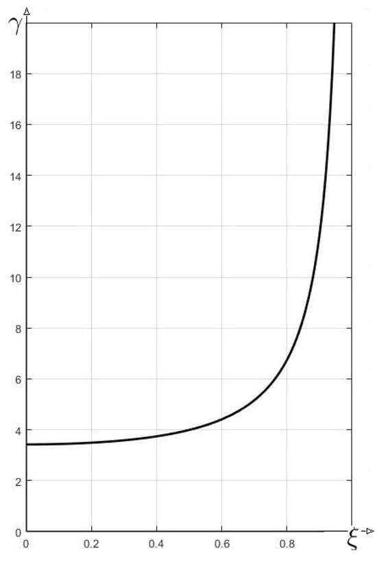
The theorem can be reformulated based on the information from the graph. If the point $(\overline{\xi },\overline{\gamma })$ lies under the curve (Figure 1), then the matrix A, with $\xi =\overline{\xi }$, $\gamma =\overline{\gamma }$ will be an M-matrix.

Figure 1. Relation graph of $\gamma$ depending of $\xi$ (formula (33)).

We also showed that in (20), both matrix A and matrix $(A+D)$ are M-matrices for $\xi \in [0,1)$ and $\gamma \in [0,{\gamma }_1)$.

5. Comparison Theorem and Construction of the Majorant Function

Our main aim is to estimate the error occurring from the nonlocal condition. In [49], based on the properties of M-matrices, a statement was proved, which is commonly referred to as the comparison theorem in the theory of finite difference method. According to this theorem, a majorant function can be formed and the error is estimated using this function.

Lemma 1 

([49]). Suppose that u and w are the solutions of two systems

$$\begin{array}{cc}\hfill & (A+D)u=f\hfill \end{array}$$

(37)

$$\begin{array}{cc}\hfill & Aw=g,\hfill \end{array}$$

(38)

respectively, where A is an M-matrix, $D\ge 0$ is diagonal matrix, and $g\ge 0$. If $\left|f\right|\le g$, then $\left|u\right|\le w$.

The solution w of the system (38) is called the majorant of the solution to the system (37).

This method for estimating the error in the solution using the majorant was introduced in 1930 by S. Gerschgorin [52]. In this paper, the Dirichlet boundary value problem for the two-dimensional Laplace equation was solved by the finite difference method.

The method, along with comments on its advantages and disadvantages, is described in detail in [53,54]. We would like to draw attention to one important aspect of the method: The comparison theorem has always been presented as a conclusion of the maximum principle [53,54,55]. The maximum principle is formulated for a system of difference equations whose matrix has the following properties:

• $a_{ij}\le 0$, $i\ne j$;
• $a_{ii}>0$;
• $a_{ii}\ge \sum \left|a_{ij}\right|$ (diagonally dominant).

It is a strong limitation. M-matrices do not require a diagonal dominance condition.

On the other hand, we must note that the result of Lemma 1, expressed in another form, essentially coincides with some results known in linear algebra (see, e.g., the discrete comparison principle in [56]). Following [56], we formulate this principle for a more general class of matrices than M-matrices.

Lemma 2 

(discrete comparison principle [56]). Let A be a monotone matrix $w\ge 0$. If $Av\le Aw$ for $v,w\in R^n$, then it follows that $v\le w$.

However, to the best of our knowledge, this principle has not actually been applied to estimate the error in the approximate solution obtained by the difference methods (except in [18,48,49]).

The expression of the majorant function is usually not commented on too much. One disadvantage of using this method to estimate the error by the construction of the majorant is that, except in some simple cases, it is not clear how to construct the majorant itself.

We construct the majorant of the solution for the system (20) in the following form:

$$w(x,y)={\displaystyle \frac{h^{2}M(1+\gamma )}{24}}\left(K-{\left(x-{\displaystyle \frac{1}{2}}\right)}^2-{\left(y-{\displaystyle \frac{1}{2}}\right)}^2+ax\right),$$

(39)

where $K\ge {\displaystyle \frac{3}{2}}$, $a\ge 0$ are constants, whose values, in the general case, depend on $\xi$ and $\gamma$. $M=max(M_2,M_4)$.

We note that under conditions $K\ge {\displaystyle \frac{3}{2}}$, $a\ge 0$, there will always be

$$w(x_i,y_j)\ge 0,i,j=0,1,\dots ,N.$$

(40)

We investigate for which values of $\xi$ and $\gamma$ function (39) $w(x,y)$ will be the majorant of the solution $z_{ij}$ of the system (20). For this, we must write the analogue of Equations (17)–(19) for the function $w(x,y)$.

Thus, knowing the matrix A and the vector $w=\left\{w_{ij}\right\}$, we construct the system $Aw=g$, i.e., we estimate the coordinates of the vector $g=\left\{g_{ij}\right\}$, where $i,j=1,2,\dots ,N-1$. First, we write down the system of equations in the form (17)–(19) for the solution $w(x,y)$. It follows from (39) that

$$\begin{array}{cc}\hfill & {\displaystyle \frac{{\partial }^{2}w}{\partial x^2}}={\displaystyle \frac{{\partial }^{2}w}{\partial y^2}}=-{\displaystyle \frac{h^{2}M(1+\gamma )}{12}},\hfill \\ \hfill & -{\displaystyle \frac{w_{i+1,j}-2w_{ij}+w_{i-1,j}}{h^2}}-{\displaystyle \frac{w_{i,j+1}-2w_{ij}+w_{i,j-1}}{h^2}}={\displaystyle \frac{{\partial }^{2}w}{\partial x^2}}+{\displaystyle \frac{{\partial }^{2}w}{\partial y^2}}.\hfill \end{array}$$

From here, we obtain the analogous equation to Equation (17) for the function $w(x,y)$.

$$-{\displaystyle \frac{w_{i+1,j}-2w_{ij}+w_{i-1,j}}{h^2}}-{\displaystyle \frac{w_{i,j+1}-2w_{ij}+w_{i,j-1}}{h^2}}={\displaystyle \frac{h^{2}M(1+\gamma )}{6}},i,j=0,1,2,\dots ,N-1.$$

(41)

Now, we will derive a simple sufficient condition under which the function $w(x,y)$, defined by formula (29), will be the majorant of $z_{ij}$. For this, we denote

$$g_{Nj}(\xi ,\gamma )=w_{Nj}-h\gamma \left({\displaystyle \frac{w_{mj}+w_{Nj}}{2}}+\sum _{i=m+1}^{N-1}{w}_{ij}\right),j=1,2,\dots ,N-1,$$

(42)

where $\xi =mh$, $1=Nh$.

The equivalent of conditions (19) for the function $w(x,y)$ is

$$w_{i0}=w(x_i,0),w_{iN}=w(x_i,1),w_{0j}=w(0,y_j).$$

(43)

Further, the difference equation system (41)–(43) for the function $w(x,y)$ is written in the form $Aw=g$. To achieve this, we express from Equation (42)

$$w_{Nj}=\sum _{i=1}^{N-1}{\alpha }_i{w}_{ij}+\beta g_{Nj}(\xi ,\gamma ),j=1,2,\dots ,N-1,$$

(44)

where ${\alpha }_i$ and $\beta$ are the same as in formula (16). After inserting these $w_{Nj}$ expressions into Equations (41), when $i=N-1$, the system (41)–(44) is transformed into the form

$$\begin{array}{cc}\hfill & -{\displaystyle \frac{w_{i+1,j}-2w_{ij}+w_{i-1,j}}{h^2}}-{\displaystyle \frac{w_{i,j+1}-2w_{ij}+w_{i,j-1}}{h^2}}={\displaystyle \frac{h^{2}M(1+\gamma )}{6}},i=1,2,\dots ,N-1,\hfill \end{array}$$

(45)

$$\begin{array}{cc}\hfill & -{\displaystyle \frac{w_{N-2,j}-2w_{N-1,j}+{\displaystyle \sum _{i=1}^{N-1}}{\alpha }_i{w}_{ij}}{h^2}}-{\displaystyle \frac{w_{N-1,j+1}-2w_{N-1,j}+w_{N-1,j-1}}{h^2}}={\displaystyle \frac{h^{2}M(1+\gamma )}{6}}+{\displaystyle \frac{\beta }{h^2}}{g}_{Nj}(\xi ,\gamma ),\hfill \end{array}$$

(46)

where $j=1,2,\dots ,N-1$.

Now, the system (45), (46), (43) can be written down in matrix form

$$Aw=g$$

(47)

analogously to how system (20) was written. Matrix A in systems (20) and (47) is the same matrix.

We should admit that to obtain the coordinate expressions of vector $g=\left\{g_{ij}\right\}$, $i,j=1,2,\dots ,N-1$, the respective values of the solution $w_{ij}$ of system (47) $w_{ij}$, $w_{i0}$, $w_{iN}$ on the contour points are not equal to zero as was characteristic for solution $z_{ij}$ of the system (20). Therefore, the values $w_{ij}$, $w_{i0}$, $w_{iN}$ should be incorporated into the expressions for $g_{ij}$. Then, we obtain

$$g_{ij}=\left\{\begin{array}{c}{\displaystyle \frac{h^{2}M(1+\gamma )}{6}}+{\displaystyle \frac{\widetilde{w_{ij}}}{h^2}}\ge {\displaystyle \frac{h^{2}M(1+\gamma )}{6}},i=1,2,\dots ,N-2,\hfill \\ {\displaystyle \frac{h^{2}M(1+\gamma )}{6}}+{\displaystyle \frac{\beta }{h^2}}{g}_{Nj}+{\displaystyle \frac{\widetilde{w_{ij}}}{h^2}}\ge {\displaystyle \frac{h^{2}M(1+\gamma )}{6}}+{\displaystyle \frac{\beta }{h^2}}{g}_{Nj},i=N-1,\hfill \end{array}\right.$$

(48)

where $\widetilde{w_{ij}}$ is one of the values $w_{ij}\ge 0$, $w_{i0}\ge 0$, and $w_{iN}\ge 0$ or is equal to zero.

We have already formulated two problems mentioned in Lemma 1. The first is the problem (20), i.e., $Az+Dz=r\left(h\right)$, with the expressions for $r\left(h\right)$

$$r_{ij}\left(h\right)=\left\{\begin{array}{c}{R}_{ij}\left(h\right),i=1,2,\dots ,N-2,j=1,2,\dots ,N-1,\hfill \\ R_{N-1,j}\left(h\right)+{\displaystyle \frac{\beta }{h^2}}{R}_{Nj},i=N-1,j=1,2,\dots ,N-1,\hfill \end{array}\right.$$

(49)

and estimates (10), (11) for $r_{ij}$. The second problem is system (47), in which $g_{ij}$ are defined by formula (48). With regard to the expressions of $r_{ij}$ and $g_{ij}$ in (20) and (47), we formulate the conclusion from Lemma 1.

Conclusion 4: If matrix A is an M-matrix, then function $w(x,y)$, defined by formula (39), is the majorant of system (20) when the condition

$$g_{Nj}\ge {\displaystyle \frac{h^{2}M(1+\gamma )}{6}}$$

(50)

is satisfied.

Indeed, for $w(x,y)$ to be the majorant of system (20), the following inequalities should be correct:

$$|r_{ij}\left(h\right)|\le g_{ij},i,j=1,2,\dots ,N-1.$$

(51)

From estimations (10) and (11), it follows that if $i=1,2,\dots ,N-2$, then

$$|r_{ij}\left(h\right)|=|R_{ij}\left(h\right)|\le {\displaystyle \frac{h^2{M}_4}{6}}\le {\displaystyle \frac{h^{2}M(1+\gamma )}{6}}\le g_{ij}$$

Further, when $i=N-1$, and from definitions (48) and (49) for $r_{N-1,j}\left(h\right)$ and $g_{N-1,j}$, it follows that

$$|r_{N-1,j}\left(h\right)|\le (1+{\displaystyle \frac{\beta }{h^2}}){\displaystyle \frac{h^{2}M(1+\gamma )}{6}}\le g_{N-1,j}$$

if only condition

$$|r_{N-1,j}\left(h\right)|\le g_{N-1,j}$$

is satisfied.

According to Conclusion 4, we have a constructive algorithm to verify, for concrete values of $\xi$ and $\gamma$, whether the function $w(x,y)$, defined by formula (39) is the majorant of the solution $z_{ij}$. On the other hand, by varying K and a, we obtain different majorants.

6. Evaluation of the Error

With reference to Lemma 1 and Conclusion 4, it is possible to evaluate the solution $z_{ij}$ of Equation (20), i.e., to evaluate the error in the approximate solution obtained by the finite difference method. To achieve this, we list some comments related to the evaluation of the error.

Firstly, it is convenient to modify inequality (50) as the sufficient condition under which $w(x,y)$ is the majorant of the system (20).

Denote

$$w^{*}(x,y)={\displaystyle \frac{1}{4}}\left(K{\left(x-{\displaystyle \frac{1}{2}}\right)}^2-{\left(y-{\displaystyle \frac{1}{2}}\right)}^2+ax\right)$$

(52)

and

$$g_{Nj}^{*}=w_{Nj}^{*}-\gamma h\left({\displaystyle \frac{w_{mj}^{*}+w_{Nj}^{*}}{2}}+\sum _{i=m+1}^{N-1}{w}_{ij}^{*}\right).$$

(53)

Then

$$w(x,y)={\displaystyle \frac{h^{2}M(1+\gamma )}{6}}{w}^{*}(x,y),g_{Nj}={\displaystyle \frac{h^{2}M(1+\gamma )}{6}}{g}_{Nj}^{*}$$

and Conclusion 4 could be reformulated as follows:

Conclusion 5: For the function $w(x,y)$, defined by formula (39), to be a majorant of system (20) with the M-matrix, the sufficient condition is

$$g_{Nj}^{*}\ge 1,$$

(54)

where $g_{Nj}^{*}$ is defined by formulas (52) and (53).

Secondly, we note that there are two variable parameters, $\xi$ and $\gamma$, in the differential problem. This complicates providing a simple and exhaustive answer to the question of which values of the parameters $\xi$ and $\gamma$ make the function $w(x,y)$, defined by formula (39), a majorant of the solution $z_{ij}$, and how to optimally choose the coefficients K and a of majorant $w(x,y)$ depending on the values of $\xi$ and $\gamma$—the authors, at least, have no consummate answer. However, by analysing the function $w(x,y)$ as a majorant, some results could be provided. First of all, we note that the function $g_{Nj}^{*}(\xi ,\gamma )$ (as well as $g_{Nj}(\xi ,\gamma )$) is monotonic with respect to both arguments.

• Function $g_{Nj}^{*}(\xi ,\gamma )$ is a monotonically increasing function with respect to the variable $\xi$ in the interval $\xi \in [0,1)$.
• Function $g_{Nj}^{*}(\xi ,\gamma )$ is a monotonically decreasing function with respect to the variable $\gamma$ in the interval $\gamma \in [0,\infty )$.

• From this monotonicity, the conclusion follows.

Conclusion 6: Provided matrix A is an M-matrix when $\xi \in [0,1)$ and $\gamma \in [0,{\gamma }_1)$ (see formula (36)). Suppose, choosing concrete $\tilde{\xi }\in [0,1)$ and $\tilde{\gamma }\in [0,{\gamma }_1)$, we obtain

$$g_{Nj}^{*}\ge 1.$$

This means that $w(x,y)$ is a majorant and the estimation of the error is as follows:

$$|z_{ij}|\le {\displaystyle \frac{h^{2}M(1+\gamma )}{6}}max\left|w^{*}(x,y)\right|\le {\displaystyle \frac{h^{2}M}{24}}(1+\gamma )(K+a)={\displaystyle \frac{MC}{24}}{h}^2,$$

(55)

where $C=(1+\gamma )(K+a)$.

The property follows from the monotonicity that

$$g^{*}(\xi ,\gamma )\ge 1$$

is true not only in the point $(\tilde{\xi },\tilde{\gamma })$, but also in the area $S=\{\tilde{\xi }\le \xi <1,0\le \gamma <\tilde{\gamma }\}$.

7. Numerical Results

We have performed a numerical experiment in order to supplement and clarify the theoretical statements on the construction of the majorant $w(x,y)$ defined by formula (39). We will use the following definitions and notations:

$$\begin{array}{cc}\hfill & S_1=\{\xi \in [0,1),\gamma \in [0,{\gamma }_1)\},\hfill \\ \hfill & {\gamma }_1=f({\beta }_0,{\xi }_0)={\displaystyle \frac{2}{h}}tanh\left({\displaystyle \frac{{\beta }_{0}h}{2}}\right){\displaystyle \frac{sinh\left({\beta }_0\right)}{cosh\left({\beta }_0\right)-cosh\left({\beta }_0{\xi }_0\right)}},\hfill \\ \hfill & {\beta }_0={\displaystyle \frac{2}{h}}ln\left(sin{\displaystyle \frac{\pi h}{2}}+\sqrt{{sin}^2{\displaystyle \frac{\pi h}{2}}+1}\right).\hfill \end{array}$$

(56)

Specifically, it was proved that, in the area $S_1$, all the eigenvalues of matrix A are real and positive:

• when $\gamma ={\gamma }_1$, then $\exists \lambda \left(A\right)=0$;
• when $\gamma >{\gamma }_1$, then $\exists \lambda \left(A\right)<0$.

In the numerical experiment, we will use a slightly stricter condition $g_{Nj}^{*}\ge 1$. Since

$$h\left({\displaystyle \frac{w_{mj}+w_{Nj}}{2}}+\sum _{i=m+1}^{N-1}{w}_{ij}\right)\le \underset{\xi }{\overset{1}{\int }}w\left(x\right)dx,when{\displaystyle \frac{{\partial }^{2}u}{\partial x^2}}\le 0,$$

then

$$g_{Nj}^{*}=w_{Nj}^{*}-\gamma h\left({\displaystyle \frac{w_{mj}^{*}+w_{Nj}^{*}}{2}}+\sum _{i=m+1}^{N-1}{w}_{ij}^{*}\right)\ge w_{Nj}^{*}-\gamma \underset{\xi }{\overset{1}{\int }}w(x,y)dx=$$

$${\displaystyle \frac{1}{4}}\left(K(1-\gamma +\gamma \xi )+\left(-{\displaystyle \frac{1}{4}}+{\displaystyle \frac{\gamma }{24}}-{\displaystyle \frac{\gamma }{3}}{\left(\xi -{\displaystyle \frac{1}{2}}\right)}^3\right)-{\left(y-{\displaystyle \frac{1}{2}}\right)}^2(1-\gamma +\gamma \xi )+a\left(1-{\displaystyle \frac{\gamma }{2}}+{\displaystyle \frac{\gamma {\xi }^2}{2}}\right)\right)\equiv {\tilde{g}}_{Nj}.$$

(57)

In formula (57) ${\tilde{g}}_{Nj}\le g_{Nj}^{*}$. Thus, the condition $g_{Nj}^{*}>1$ is stricter than the condition ${\tilde{g}}_{Nj}>1$. However, we note that ${\tilde{g}}_{Nj}\to g_{Nj}^{*}$ when $h\to 0$. Changing the condition from $g_{Nj}^{*}$ to ${\tilde{g}}_{Nj}$ makes sense, as by using the new condition in formula (57), the coefficients of a and K have a simple interpretation.

In Table 1 and Table 2, we provide some obtained combinations of the parameters ${\xi }_0$, ${\gamma }_0$, and a, when the values are $g_{Nj}^{*}\ge 1$, guaranteeing that $w(x,y)$ is a majorant function for the error $z_{ij}$. Parameter ${\gamma }_1$ was calculated according to formula (56).

Table 1. Values of ${\tilde{g}}_{Nj}\ge 1$ at ${\xi }_0=0.8$ and ${\gamma }_1=6.7445$.

${\mathit{\gamma }}_0$	$\mathit{a}=3$	$\mathit{a}=4$	$\mathit{a}=5$
${\gamma }_0=1.0$	0.811	1.016	1.221
${\gamma }_0=2.0$	0.621	0.781	0.941
${\gamma }_0=3.0$	0.432	0.547	0.662

Table 2. Values of ${\tilde{g}}_{Nj}\ge 1$ at ${\xi }_0=0.9$ and ${\gamma }_1=11.6599$.

${\mathit{\gamma }}_0$	$\mathit{a}=3$	$\mathit{a}=4$	$\mathit{a}=5$
${\gamma }_0=1.0$	0.903	1.129	1.355
${\gamma }_0=2.0$	0.805	1.008	1.210
${\gamma }_0=3.0$	0.708	0.887	1.065

Numerical calculations show that ${\tilde{g}}_{Nj}\ge 1$ for higher values of parameter ${\xi }_0$ (the lower bound of the integral nonlocal conditions), i.e., ${\xi }_0$ approaches closer to 1. Additionally, it depends on ${\gamma }_0$ which is expected to be lower.

Increasing the value of ${\gamma }_0$ towards ${\gamma }_1$ always requires a large regulative parameter a, which leads us to a greater value of the error. In Table 3, the dependence of the condition $g_{Nj}^{*}\ge 1$ on the value of the parameter a can be seen.

Table 3. Values of ${\tilde{g}}_{Nj}\ge 1$ at ${\xi }_0=0.8$ and ${\gamma }_0$$\to {\gamma }_1$.

${\mathit{\gamma }}_0/\mathit{a}$	$\mathit{a}=4$	$\mathit{a}=8$	$\mathit{a}=42$	$\mathit{a}=450$
${\gamma }_0=1.0$	1.016	1.836	8.806	92.446
${\gamma }_0=3.0$	0.547	1.007	4.917	51.837
${\gamma }_0=5.0$	0.0078	0.178	1.028	11.228
${\gamma }_0=5.5$	−0.045	−0.035	0.050	1.070
${\gamma }_0=6.0$	−0.169	−0.249	−0.929	−9.089
${\gamma }_0=6.5$	−0.292	−0.462	−1.907	−19.247

From the results in Table 1 and Table 2, we see that for relatively small $\gamma$ values, the condition ${\tilde{g}}_{Nj}\ge 1$ can be ensured by increasing K and a. However, when $\gamma$ values approach ${\gamma }_1$, (Table 3 and Table 4), the situation changes for the worse. As the values of K and a increase, the condition ${\tilde{g}}_{Nj}>1$ remains unfulfilled.

Table 4. Values of ${\tilde{g}}_{Nj}$ (${\xi }_0=0.9$), $\overline{\gamma }=10.5263$, ${\gamma }_1=11.6599$.

${\mathit{\gamma }}_0/\mathit{a}$	$\mathit{a}=3.5$	$\mathit{a}=7$	$\mathit{a}=28$	$\mathit{a}=85$	$\mathit{a}=1750$
${\gamma }_0=1.0$	1.016	1.808	6.559	19.455	3.96161
${\gamma }_0=5.0$	0.579	1.038	3.794	11.275	229.807
${\gamma }_0=9.0$	0.141	0.268	1.030	3.096	63.452
${\gamma }_0=10.0$	0.032	0.076	0.338	1.051	21.863
${\gamma }_0=10,5$	−0.026	−0.024	−0.010	0.025	1.066
${\gamma }_0=11.0$  ${\gamma }_0\ge \overline{\gamma }$	−0.083	−0.123	−0.359	−1.000	−19.732

As in the expression of the ${\tilde{g}}_{Nj}$ coefficient to a

$$1-{\displaystyle \frac{{\gamma }_0}{2}}+{\displaystyle \frac{{\gamma }_0{\xi }_0^2}{2}}>0,\mathrm{when}0<{\gamma }_0<{\displaystyle \frac{2}{1-{\xi }_0^2}},$$

then for the fixed values of $\xi$ and $\gamma$, the value of ${\tilde{g}}_{Nj}$ increases as parameter a increases. Thus, for the fixed ${\xi }_0$ and ${\gamma }_0$, the function $w(x,y)$ will always be a majorant only if the coefficient to parameter a in (57) is positive. Parameter a increases without bound and ${\gamma }_0<\overline{\gamma }={\displaystyle \frac{2}{1-{\xi }_0^2}}$.

When ${\gamma }_0\ge \overline{\gamma }$, the coefficient to parameter a becomes negative, and $w(x,y)$ is no longer a majorant, as can be seen in Table 3 and Table 4.

The conclusion follows from (57):

Conclusion 7: The larger the value ${\gamma }_0$, the larger the value of the parameter a, and thus the larger the value of C in estimating the error $z_{ij}$ (see formula (55)).

8. Conclusions and Generalization

This paper analysed which values of the parameters $\xi$ and $\gamma$ make the matrix of the system of difference equations an M-matrix. By applying M-matrix theory, the convergence conditions of iterative methods for solving the system of nonlinear equations were determined. If the matrix of the difference equation system is an M-matrix, many iterative methods converge [18].

If the matrix of the system of difference equations is an M-matrix, then we can construct a majorant function to estimate the error in the solution for any parameter $\xi \in [0,1)$. However, numerical results indicate that this is only true under a certain combination of the parameters $\xi$ and $\gamma$. As the parameter $\gamma$ increases, it is necessary to increase the parameter a as well, which leads to greater error. Numerical results show the same effect if we decrease the parameter $\xi$ towards zero.

In expression (39) of the majorant function $w(x,y)$, we used the regulative member $ax$, which ensures that $w^{*}(x,y)\ge 0$.

The construction of the majorant (according to S. Gerschgorin [52,53,54,55]), based on M-matrix theory, is a suitable method for estimating the error in the finite difference method when solving boundary value problems for elliptic equations with nonlocal conditions.

We would like to provide a few more comments on the applications of M-matrix theory used in this paper for the investigation of difference schemes. The concept of the M-matrix [50] and the proof of convergence of the difference scheme by constructing the majorant [52] appeared around the same time in the fourth decade of the last century. In 1962, in the monograph of R. S. Varga [51], considering the application of Perron–Frobenius non-negative matrix theory to the investigation of difference schemes for elliptic and parabolic equations, M-matrices were already mentioned. However, the role of M-matrices in solving differential equations with classical Dirichlet and Neumann conditions was not substantial.

With the introduction of new mathematical models with nonlocal conditions, new research methods were needed. Here, it became clear that the theory of M-matrices is one of the suitable models for composing and analysing numerical methods for problems with nonlocal conditions.

Using the regular splitting principle [50,57], well known in linear algebra, it is possible to create convergent iterative methods for difference equation systems with nonlocal conditions [18]. However, the proof of the convergence of difference schemes based on the construction of a majorant has one shortcoming [54]—there is no algorithm for explicitly constructing the majorant. Nevertheless, when applying the theory of M-matrices in this paper, the situation is better. According to the properties of M-matrices, a vector $x>0$ exists such that $Ax>0$ for an M-matrix A. It is not difficult to verify that, from there, it follows that the majorant exists.

The method of proof for the convergence of the difference schemes provided in this paper is also applicable to many other equations, boundary conditions, or numerical methods—for instance, solving the system of Equations (1)–(3) using the finite element method with linear elements. It is important that it is possible to formulate the difference problem with an M-matrix (one such problem is the Poisson equation with an integral Neumann condition). Of course, the M-matrix method is not universal (for example, it is not suitable for problem (1)–(3) when $\gamma <0$), but its potential is far from exhausted.

References

- Cannon, J.R. The solution of the heat equation subject to the specification of energy. Q. Appl. Math. 1963, 21, 155–160. [Google Scholar] [CrossRef]
- Kamynin, L.I. A boundary value problem in the theory of heat conduction with a nonclassical boundary condition. Comput. Math. Math. Phys. 1964, 4, 33–59. [Google Scholar] [CrossRef]
- Day, W.A. Extensions of a property of the heat equation to linear thermoelasticity and other theories. Q. Appl. Math. 1982, 40, 319–330. [Google Scholar] [CrossRef]
- Ionkin, N. Solution of one boundary value problem of the theory of heat conduction with a nonclassical boundary condition. Differ. Equ. 1977, 13, 204–211. [Google Scholar]
- Skubachevskii, A.L. Nonlocal elliptic problems in infinite cylinder and applications. Discret. Contin. Dyn. Syst. Ser. S 2016, 9, 847–868. [Google Scholar] [CrossRef]
- Dehghan, M. Efficient techniques for the second-order parabolic equation subject to nonlocal specifications. Appl. Numer. Math. 2005, 52, 39–62. [Google Scholar] [CrossRef]
- Ma, R. A Survey On Nonlocal Boundary Value Problems. Appl. Math. E-Notes 2007, 7, 257–279. [Google Scholar]
- Štikonas, A. A survey on stationary problems, Green’s functions and spectrum of Sturm-Liouville problem with nonlocal boundary conditions. Nonlinear Anal. Model. Control 2014, 19, 301–334. [Google Scholar] [CrossRef]
- Bitsadze, A.V.; Samarskii, A.A. On some simple generalizations of linear elliptic problems. Sov. Math. Dokl. 1969, 185, 398–400. [Google Scholar]
- Ashyralyev, A.; Ozturk, E. On a difference scheme of second order of accuracy for the Bitsadze-Samarskii type nonlocal boundary-value problem. Bound. Value Probl. 2014, 2014, 14. [Google Scholar] [CrossRef]
- Avalishvili, G.; Avalishvili, M.; Gordeziani, D. On a nonlocal problem with integral boundary conditions for a multidimensional elliptic equation. Appl. Math. Lett. 2011, 14, 566–571. [Google Scholar] [CrossRef]
- Berikelashvili, G.K.; Khomeriki, N. On the convergence rate of a difference solution of the Poisson equation with fully nonlocal constraints. Nonlinear Anal. Model. Control 2014, 19, 367–381. [Google Scholar] [CrossRef]
- Pao, C. Numerical solutions of reaction–diffusion equations with nonlocal boundary conditions. J. Comput. Appl. Math. 2001, 136, 227–243. [Google Scholar] [CrossRef]
- Feng, C.; Nie, C.; Yu, H.; Zhou, L. A Difference Scheme and Its Error Analysis for a Poisson Equation with Nonlocal Boundary Conditions. Complexity 2020, 2020, 6329404. [Google Scholar] [CrossRef]
- Sapagovas, M. Difference method of increased order of accuracy for the Poisson equation with nonlocal conditions. Differ. Equ. 2008, 44, 1018–1028. [Google Scholar] [CrossRef]
- Dosiyev, A.A. Difference method of fourth order accuracy for the Laplace equation with multilevel nonlocal conditions. J. Comput. Appl. Math. 2019, 354, 587–596. [Google Scholar] [CrossRef]
- Zhou, L.; Yu, H. Error estimate of a high accuracy difference scheme for Poisson equation with two integral boundary conditions. Adv. Differ. Equ. 2018, 2018, 225. [Google Scholar] [CrossRef]
- Sapagovas, M.; Griškonienė, V.; Štikonienė, O. Application of M-matrices for solution of a nonlinear elliptic equation with an integral condition. Nonlinear Anal. Model. Control 2017, 22, 489–504. [Google Scholar] [CrossRef]
- Sapagovas, M.; Pupalaigė, K.; Čiupaila, R.; Meškauskas, T. On the spectrum structure for one difference eigenvalue problem with nonlocal boundary conditions. Math. Model. Anal. 2023, 28, 522–541. [Google Scholar] [CrossRef]
- Štikonienė, O.; Sapagovas, M. Alternating direction implicit method for Poisson equation with integral conditions. Math. Model. Anal. 2023, 28, 715–734. [Google Scholar] [CrossRef]
- Pečiulytė, S.; Štikonienė, A.; Štikonas, O. Sturm-Liouville problem for stationary differential operator with nonlocal integral boundary condition. Math. Model. Anal. 2005, 10, 377–392. [Google Scholar] [CrossRef]
- Bingelė, K.; Bankauskienė, A.; Štikonas, A. Spectrum curves for a discrete Sturm-Liouville problem with one integral boundary condition. Nonlinear Anal. Model. Control 2019, 24, 755–774. [Google Scholar] [CrossRef]
- Pupalaigė, K.; Sapagovas, M.; Čiupaila, R. Nonlinear elliptic equation with nonlocal integral boundary condition depending on two parameters. Math. Model. Anal. 2022, 27, 610–628. [Google Scholar] [CrossRef]
- Bingelė, K.; Bankauskienė, A.; Štikonas, A. Investigation of spectrum curves for a Sturm–Liouville problem with two-point nonlocal boundary conditions. Math. Model. Anal. 2020, 25, 53–70. [Google Scholar] [CrossRef]
- Gao, J.; Sun, D.; Zhang, M. Structure of Eigenvalues of Multi-Point Boundary Value Problems. Adv. Differ. Equ. 2010, 2010, 381932. [Google Scholar] [CrossRef]
- Sergejeva, N.; Pečiulytė, S. On Fučik type spectrum for problem with integralnonlocal boundary condition. Nonlinear Anal. Model. Control 2019, 24, 261–278. [Google Scholar] [CrossRef]
- Pečiulytė, S.; Štikonienė, O.; Štikonas, A. Investigation of negative critical point of the characteristic function for problems with nonlocal boundary conditions. Nonlinear Anal. Model. Control 2008, 13, 464–490. [Google Scholar] [CrossRef]
- Štikonas, A.; Štikonienė, O. Characteristic Functions for Sturm–Liouville Problems with Nonlocal Boundary Conditions. Math. Model. Anal. 2009, 14, 229–246. [Google Scholar] [CrossRef]
- Štikonas, A.; Şen, E. Asymptotic analysis of Sturm-Liouville problem with nonlocal integral type boundary condition. Nonlinear Anal. Model. Control 2021, 26, 969–991. [Google Scholar] [CrossRef]
- Sapagovas, M.P. Numerical methods for two-dimensional problem with nonlocal conditions. Differ. Equ. 1984, 20, 926–933. [Google Scholar]
- Jeknič, Z.M.; Sredojevič, B.; Bojovič, D. On the numerical solution of an elliptic problem with nonlocal boundary conditions. Electron. Trans. Numer. Anal. 2023, 59, 179–201. [Google Scholar] [CrossRef]
- Koleva, M. Finite element solution ofboundary value problems with nonlocal jump conditions. Math. Model. Anal. 2008, 13, 383–400. [Google Scholar] [CrossRef]
- Nie, C.; Yu, H. Some error estimates on the finite element approximation for two-dimensional elliptic problem with nonlocal boundary. Appl. Numer. Math. 2013, 68, 31–38. [Google Scholar] [CrossRef]
- Nikolopoulos, C.; Zouraris, G. Numerical Solution of a Non-Local Elliptic Problem Modeling a Thermistor with a Finite Element and a Finite Volume Method. In Progress in Industrial Mathematics at ECMI 2006. Mathematics in Industry; Bonilla, L.L., Moscoso, M., Platero, G., Vega, J.M., Eds.; Springer: Berlin/Heidelberg, Germany, 2008; Volume 12. [Google Scholar] [CrossRef]
- Nie, C.; Shu, S.; Yu, H.; An, Q. A high order composite scheme for the second order elliptic problem with nonlocal boundary and its fast algorithm. Appl. Math. Comput. 2014, 227, 212–221. [Google Scholar] [CrossRef]
- Chen, H.; Stynes, M. A discrete comparison principle for the time-fractional diffusion equation. Comput. Math. Appl. 2020, 80, 917–922. [Google Scholar] [CrossRef]
- Wang, Y.; Zhao, Y.; Chen, H. Discrete comparison principle of a finite difference method for the multi-term time fractional diffusion equation. Numer. Algorithms 2022, 93, 1581–1593. [Google Scholar] [CrossRef]
- Chen, Y.; Zhang, J.; Huang, Y.; Xu, Y. A posteriori error estimates of hp spectral element methods for integral state constrained elliptic optimal control problems. Appl. Numer. Math. 2019, 2019, 42–58. [Google Scholar] [CrossRef]
- Chen, Y.; Yi, N.; Liu, W. A Legendre—Galerkin spectral method for optimal control problems governed by elliptic equations. SIAM J. Numer. Anal. 2008, 46, 2254–2275. [Google Scholar] [CrossRef]
- Sajavičius, S. Radial basis function method for a multidimensional linear elliptic equation with nonlocal boundary conditions. Comput. Math. Appl. 2014, 67, 1407–1420. [Google Scholar] [CrossRef]
- Boutayeb, A.; Chetouani, A. A numerical comparison of different methods applied to the solution of problems with non local boundary conditions. Appl. Math. Sci. 2007, 1, 2173–2185. [Google Scholar]
- Agarwal, P.; Merker, J.; Schuldt, G. Singular Integral Neumann Boundary Conditions for Semilinear Elliptic PDEs. Axioms 2021, 10, 74. [Google Scholar] [CrossRef]
- Merker, J. Very weak solutions of linear elliptic PDEs with singular data and irregular coefficients. Differ. Equ. Appl. 2018, 10, 3–20. [Google Scholar] [CrossRef]
- Li, Y.; O’Regan, D.; Xu, J. Existence of solutions for a fractional Riemann–Stieltjes integral boundary value problem. Nonlinear Anal. Model. Control 2024, 29, 488–508. [Google Scholar] [CrossRef]
- Nguyen, V.T. On Caputo fractional elliptic equation with nonlocal condition. Adv. Theory Nonlinear Anal. Appl. 2023, 7, 205–214. [Google Scholar] [CrossRef]
- Shakhmurov, V.; Kurulay, M. Nonlocal fractional elliptic equations and applications. Numer. Meth. Part. Differ. Equ. 2023, 39, 821–1798. [Google Scholar] [CrossRef]
- El-Sayed, A.M.A.; El-Gendy, M.E.I. Solvability of a Stochastic Differential Equation with Nonlocal and Integral Conditions. Differ. Equ. Control Process. 2017, 3, 47–59. [Google Scholar]
- Sapagovas, M.; Novickij, J. On stability in the maximum norm of difference scheme for nonlinear parabolic equation with nonlocal condition. Nonlinear Anal. Model. Control 2023, 28, 365–376. [Google Scholar] [CrossRef]
- Sapagovas, M.; Štikonienė, O.; Jakubėlienė, K.; Čiupaila, R. Finite difference method for boundary value problem for nonlinear elliptic equation with nonlocal conditions. Bound. Value Probl. 2019, 2019, 9. [Google Scholar] [CrossRef]
- Berman, A.; Plemmons, R. Nonnegative Matrices in the Mathematical Sciences; SIAM: Philadelphia, PA, USA, 1994. [Google Scholar]
- Varga, R. Matrix Iterative Analysis, 2nd ed.; Springer Series in Computational Mathematics; Springer: Berlin/Heidelberg, Germany, 2000; Volume 27. [Google Scholar]
- Gerschgorin, S. Fehlerabschatzung fur das Differenzenverfahren zur Losung partieller Differentialgleichungen. Z. Angew. Math. Mech. 1930, 10, 379–382. [Google Scholar] [CrossRef]
- Collatz, L. Numerische Behandlung von Differentialgleichungen, 2nd ed.; Springer: Berlin/Gottingen/Heidelberg, Germany, 1953. [Google Scholar]
- Forsythe, G.E.; Wasow, W.R. Finite–Difference Methods for Partial Differential Equations; John Wiley Sons: New York, NY, USA; London, UK, 1960. [Google Scholar]
- Samarskii, A.A. The Theory of Difference Schemes; CRC Press: New York, NY, USA, 2001. [Google Scholar]
- Volker, J. Numerical Mathematics; Weierstrass Institute for Applied Analysis and Stochastics: Berlin, Germany, 2022; Lecture Notes, Chapter 5. [Google Scholar]
- Franco, D.; Infante, G.; Minhós, F.M. Nonlocal boundary value problems. Bound. Value Probl. 2012, 2012, 23. [Google Scholar] [CrossRef]
Disclaimer/Publisher’s Note: The statements, opinions and data contained in all publications are solely those of the individual author(s) and contributor(s) and not of MDPI and/or the editor(s). MDPI and/or the editor(s) disclaim responsibility for any injury to people or property resulting from any ideas, methods, instructions or products referred to in the content. |
© 2025 by the authors. Licensee MDPI, Basel, Switzerland. This article is an open access article distributed under the terms and conditions of the Creative Commons Attribution (CC BY) license (https://creativecommons.org/licenses/by/4.0/).