Nonlinear Stochastic Modeling with Heterogeneous Covariates for Degradation Analysis Applied to Wax Lubrication Layer

Abstract

Wax is a commonly used lubricant in many applications. To ensure its security and dependability, degradation analyses for creep are typically conducted. However, challenges arise due to the poorly understood inherent mechanisms of wax and the complicated experimental environment required, leading to nonlinear trends and heterogeneous covariates. In such cases, traditional methods based on parametric forms or linear assumptions may lack the flexibility to capture the complexities and randomness of the degradation process effectively. To address these challenges, we propose a comprehensive degradation analysis framework that employs a Wiener process with an unspecified mean function. By eliminating parametric forms, this approach offers a more versatile way to model nonlinear degradation trends. Moreover, it treats environmental covariates as random variables to handle random environmental influences. We develop tailored semiparametric estimators for the model and establish theoretical asymptotic results that guarantee the consistency and convergence of the proposed estimators. A series of numerical experiments are conducted to illustrate the performance of the estimators and validate their convergence properties. The method is applied to a wax lubrication layer, demonstrating its efficacy in analyzing nonlinear degradation data in a random working environment. This work advances the understanding of wax degradation mechanisms and provides a flexible tool for degradation analysis in materials with heterogenic environments and poorly understood behaviors.

1. Introduction

1.1. Background

Failures in operational systems can result in substantial financial losses and potentially catastrophic outcomes. Therefore, developing a robust framework for understanding and assessing system reliability is crucial to mitigating risks and enhancing safety, performance, and operational efficiency. Degradation is a primary cause of failure in numerous industrial systems, such as wind power generators [1], six-DoF robots [2], and high-power semiconductor lasers [3]. By modeling and understanding degradation patterns and mechanisms, estimating the remaining useful life (RUL) or reliability of the system, and informing decisions related to maintenance, repair, or replacement strategies, degradation analysis provides a foundation for proactive system management. These efforts are essential for ensuring system longevity and minimizing downtime.

Let us consider a product with a critical performance characteristic (PC), denoted by $X\left(t\right)$, that degrades over time. When the degradation of the PC exceeds a predefined threshold level, the product or system is considered to be failed [4]. This degradation-threshold failure mechanism establishes a direct link between degradation patterns and product failures. Since the PC is intrinsically tied to the product’s lifespan, modeling its degradation offers a robust approach to assessing the product’s reliability. By analyzing the degradation mechanism and the corresponding data, the failure time distribution and its parameters can be estimated, providing valuable insights for reliability assessment and maintenance planning. In the following subsection, we present a specific motivating example related to the wear layer to illustrate the practical application of this degradation-threshold framework.

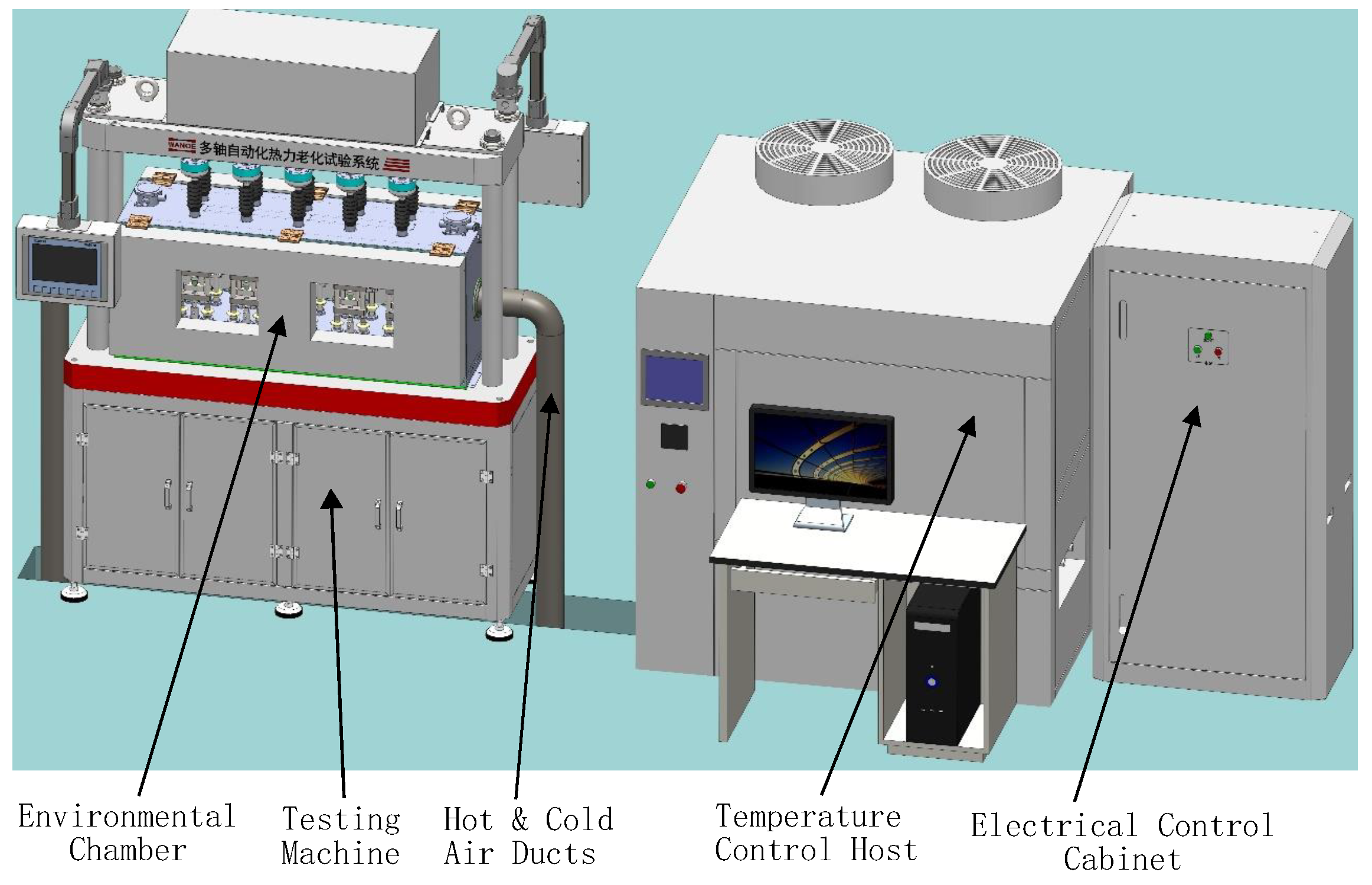
1.2. Motivating Example

The safety of the storage and transportation of explosives has always been a critical priority, with significant implications for environmental preservation and public safety. One effective approach to enhancing safety is the application of a protective coating on the surface of the explosive. This coating reduces direct friction between the explosive column and the metal shell, which contributes to the overall operational safety of press-packed explosives, mitigating risks and ensuring safer handling and storage. In this regard, wax has proven to be quite useful in reducing the sensitivity of explosives to outside stimuli due to its function as a lubricating layer [5,6]. Beyond its economic and practical merits, wax distinguishes itself due to its superior capacity to disperse across crystal surfaces from other desensitizing materials. This attribute ensures the thorough encapsulation of energetic crystals, increasing their safety and stability [7,8].

However, the deformation of the wax layer reduces the thickness of the lubrication interface, amplifying the safety risks associated with explosives [9]. When subjected to deformation, the wax lubrication layer exhibits complex and nonlinear creep behavior, which can be divided into three distinct stages: the initial elastic response, the subsequent creep phase (characterized by slow deformation), and the eventual abrupt fracture of the structure [10]. Conventional models, such as the Burger mechanical-analogy model, have limitations in accurately describing these nonlinear creep phenomena in the wax lubrication layer [11]. On the other hand, working conditions, particularly temperature, significantly accelerate the degradation of the wax lubrication layer encapsulating explosive crystals. A critical aspect to note is that the degradation trends are heavily influenced by different covariates, exhibiting complex and nonlinear behavior, as illustrated in Figure 1. Furthermore, during the data collection process, the working environment often deviates from preset conditions, introducing heterogeneity in the covariates. These factors pose significant challenges in accurately modeling the degradation of the wax lubrication layer, highlighting the need for advanced approaches to capturing the intricate relationships between covariates and degradation behavior.

1.3. Literature Review

For degradation analysis, there are primarily two kinds of models used to fit the degradation data of the PC. The first type employs regression analysis, wherein the degradation measurements are described by the equation $X\left(t\right)=\mathsf{\Gamma }(t;\mathit{\alpha })+\epsilon$. In this model, the true degradation path depends on unknown parameters $\mathit{\alpha }$ and $\epsilon \sim N(0,{\sigma }_e^2)$. Several variants of this model have been developed, including those proposed by [12,13,14]. For further details on this type of model, please refer to [15] and the references therein.

The second type considers the degradation path as the result of an accumulation of infinitesimal segments, leading to the use of stochastic process models. Unlike the general path model, these models effectively address the randomness introduced by inherent variability and environmental factors in the degradation process. Three commonly employed stochastic processes in this context are the Wiener process [16,17,18], the gamma process [19,20,21], and the inverse Gaussian process [22,23,24]. These processes are well suited for characterizing the dynamics and uncertainties of degradation due to their time-dependent structural properties [25]. Among these, the Wiener process is particularly prominent for its flexibility and versatility in the analysis of degradation data [26,27,28,29].

Linearization methods, such as state transformations [30], have been proposed in the literature, but they often fall short in addressing all scenarios due to their limited efficiency [18]. This limitation stems from the inherent nonlinearity in system degradation, which arises from complex operational environments and intricate failure mechanisms [31,32]. A widely recognized approach for addressing nonlinear degradation involves using specific parametric forms for the mean function, such as power law, exponential, and logarithmic functions [29,33,34]. However, selecting the most appropriate model presents significant challenges [35], and these parametric forms may not fully capture the true degradation path. To overcome this limitation, nonparametric techniques can be employed, offering greater flexibility and accuracy in modeling complex degradation behaviors. To the best of our knowledge, the literature on nonparametric methods for modeling degradation paths is quite limited. The authors of [36,37] introduced nonparametric estimators for the mean function based on the pseudo-likelihood approach. However, these estimators may exhibit inefficiencies due to the inherent limitations of the pseudo-likelihood framework. The authors in [38] extended this method to handle multiple dependent degradation paths. However, the proposed model may be overly complex for a single performance characteristic $X\left(t\right)$.

On the other hand, certain covariates, such as the working temperature, significantly influence system degradation and should be incorporated into the model. A natural approach is to assume that the degradation path is a function of covariates with associated parameters [18]. For example, the authors of [39] proposed a degradation model based on the exponential-dispersion process with covariates, while the authors in [15] analyzed NIST coating degradation data by using a general path model that includes covariates. For a comprehensive review of such approaches, one can refer to [40]. Furthermore, heterogeneity in degradation data complicates the identification of consistent degradation patterns and increases uncertainty in reliability assessments. This underscores the need for advanced modeling techniques to effectively address these complexities and improve the accuracy of degradation modeling and lifetime prediction. A few studies in the literature, such as [12,20,41], have considered heterogeneity, but their focus has primarily been on inherent differences between units rather than heterogeneity caused by working environments. To the best of our knowledge, there is no model for the creep behavior of the wax lubrication layer simultaneously considering the unknown underlying mechanisms and the heterogeneity introduced by the working environment.

1.4. Contribution and Outline

This study focuses on the critical problem of modeling the degradation of the wax lubrication layer, particularly under the influence of temperature, which plays a significant role in system reliability. The primary challenge stems from the lack of an understanding of the physical mechanisms governing the wax lubrication layer, combined with the heterogeneity introduced by varying working conditions. These factors complicate the accurate modeling of degradation and the prediction of system lifetime, highlighting the need for a robust and flexible approach. To overcome these challenges, we propose a novel method based on a Wiener process with a nonlinear function of time which does not rely heavily on a clear physical mechanism. This approach incorporates random covariates to effectively capture the heterogeneity caused by the working environment. The proposed method achieves significant improvements in modeling accuracy and reliability prediction, offering a robust framework for addressing the complexities of degradation in wax lubrication layers under real-world conditions. The main contributions of this work can be summarized as follows:

(1)

By addressing the challenge of modeling the unknown and nonlinear behavior of wax creep under the influence of temperature, we provide a comprehensive analysis of this complex phenomenon.

(2)

By utilizing a new degradation model based on the Wiener process, we describe the inherent relationships between creep and time without assuming a specific parametric form.

(3)

By considering that the working environment is different even if the covariates preset are the same, we view covariates as random variables to capture the heterogeneity among degradation data.

(4)

We propose a nonparametric estimator to estimate the nonlinear function concerning time and derive the corresponding asymptotic results.

The remainder of this article is organized as follows: In Section 2, we introduce a nonlinear stochastic model that incorporates random covariates based on the Wiener process. We propose a nonparametric estimation method to estimate the mean function, with knots occurring only at measurement times. The expectation–maximization algorithm is also developed. We then present several asymptotic results for the estimator. Some numerical experiments are conducted, as reported in Section 3, to validate the proposed method. In Section 4, we describe the application of our approach to wax creep data. Concluding remarks are provided in Section 5. Technical proofs and additional simulation results are included in the Supplementary Materials.

2. Methodology

In this section, we first present the Wiener process model for degradation analysis with a nonlinear trend modeled including heterogeneous covariates. We then derive the estimators based on maximum likelihood (ML) and study their corresponding asymptotic properties. The expectation–maximization (EM) algorithm is also established for the estimation.

2.1. Nonlinear Wiener Process Models

Let us assume that the environmental stress, which is also referred to as covariates hereafter, under which the product operates is denoted by $\mathit{Z}={[Z_1,\cdots ,Z_d]}^{\top }$ and includes factors such as the temperature of the environment in which the wax lubrication layer is situated.

To capture the nonlinear degradation characteristics influenced by the covariates, we consider a Wiener process with a nonlinear trend which is given by

$$X(t,\mathit{Z})=H(t,\mathit{Z})+\sigma \mathcal{B}\left(H\right(t,\mathit{Z}\left)\right),$$

(1)

where $H(·)$ denotes the degradation trend, which is a positive and non-decreasing function with $H\left(0\right|\mathit{Z})=0$; $\sigma >0$ denotes the diffusion parameter; $\mathcal{B}(·)$ denotes standard Brownian motion; and t represents the measurement time. The Wiener process is widely used in degradation modeling due to its strong physical interpretation and favorable statistical properties. For many products, degradation increments over infinitesimal time intervals can be viewed as the cumulative result of numerous small, independent external effects. By the central limit theorem, the aggregate of these effects tends to follow a normal distribution, making the Wiener process a natural choice for modeling such behavior. Additionally, the Wiener process provides a continuous-time stochastic framework that captures both the deterministic trend (drift) and the inherent randomness (diffusion) in degradation processes. This dual representation allows for a comprehensive understanding of degradation dynamics, enabling probabilistic predictions and uncertainty quantification. Thus, the Wiener process, characterized by normally distributed increments, is a proper and effective model in the study of degradation analysis.

To model the relationship between degradation and covariates, we employ the Cox proportional hazards model to link covariates to trend $H(·)$. The model is expressed as

$$X(t;\mathit{Y})=\mathsf{\Lambda }\left(t\right)exp\left({\mathit{\beta }}^{\top }\mathit{Y}\right)+\sigma \mathcal{B}\left(\mathsf{\Lambda }\left(t\right)exp\left({\mathit{\beta }}^{\top }\mathit{Y}\right)\right),$$

(2)

where $\mathsf{\Lambda }(·)$ denotes the degradation trend, which is a positive and increasing function with $\mathsf{\Lambda }\left(0\right)=0$; $\mathit{\beta }={[{\beta }_1,\cdots ,{\beta }_d]}^{\top }$ is a column vector of unknown coefficients to measure the influence of $\mathit{Y}$; and $\mathit{Y}={[Y_1,\cdots ,Y_d]}^{\top }$ is a vector of random variables that depends on covariates $\mathit{Z}$. The reason for introducing Y is that even if under identical preset conditions, the working environment of individual units exhibits stochastic variations around the fixed values. Specifically, $Y_i=Z_i+{ϵ}_i$, with ${ϵ}_i\sim N(0,{\gamma }_i^2)$. Then, noticing that the underlying physical mechanism is unknown, we further release additional specific functional forms for $\mathsf{\Lambda }(·)$ to improve flexibility. Overall, we propose a Wiener process-based degradation model that integrates a nonlinear degradation path and stochastic covariates.

For a given $\mathit{Y}$, the Wiener process model ensures that the degradation increments, $X(t+\Delta t)-X\left(t\right)$, are independent and follow Gaussian distributions:

$$X(t+\Delta t)-X\left(t\right)|\mathit{Y}\sim N\left(\lambda (\Delta t)exp\left({\mathit{\beta }}^{\top }\mathit{Y}\right),{\sigma }^2\lambda (\Delta t)exp\left({\mathit{\beta }}^{\top }\mathit{Y}\right)\right),$$

where $\lambda (\Delta t)=\mathsf{\Lambda }(t+\Delta t)-\mathsf{\Lambda }\left(t\right).$ Due to the independence among all covariates, ${\mathit{\beta }}^{\top }\mathit{Y}$ follows a univariate normal distribution with mean ${\mathit{\beta }}^{\top }\mathit{Z}$ and variance ${\mathit{B}}^{\top }\mathbf{\Gamma }$, with $\mathbf{\Gamma }={[{\gamma }_1^2,\cdots ,{\gamma }_d^2]}^{\top }$ and $\mathit{B}={[{\beta }_1^2,\cdots ,{\beta }_d^2]}^{\top }$. Let $R=\lambda (\Delta t)exp\left({\mathit{\beta }}^{\top }\mathit{Y}\right)$. Then, we have $lnR={\mathit{\beta }}^{\top }\mathit{Y}+ln\lambda (\Delta t)\sim N(ln\lambda (\Delta t)+{\mathit{\beta }}^{\top }\mathit{Z},{\mathit{B}}^{\top }\mathbf{\Gamma })$. Thus, R follows a log-normal distribution with the following probability density function (PDF):

$$f_R\left(r\right)={\displaystyle \frac{1}{r}}{\displaystyle \frac{1}{\sqrt{2\pi {\mathit{B}}^{\top }\mathbf{\Gamma }}}}exp\left(-{\displaystyle \frac{{(lnr-ln\lambda (\Delta t)-{\mathit{\beta }}^{\top }\mathit{Z})}^2}{2{\mathit{B}}^{\top }\mathbf{\Gamma }}}\right).$$

The PDF of $X(t+\Delta t)-X\left(t\right)$ can be formulated as

$$\begin{array}{cc}\hfill f(x;\Delta t)& =\int {\displaystyle \frac{1}{\sqrt{2\pi {\sigma }^{2}r}}}exp\left(-{\displaystyle \frac{{(x-r)}^2}{2{\sigma }^{2}r}}\right){\displaystyle \frac{1}{r}}{\displaystyle \frac{1}{\sqrt{2\pi {\mathit{B}}^{\top }\mathbf{\Gamma }}}}exp\left(-{\displaystyle \frac{{(lnr-ln\lambda (\Delta t)-{\mathit{\beta }}^{\top }\mathit{Z})}^2}{2{\mathit{B}}^{\top }\mathbf{\Gamma }}}\right)dr\hfill \\ \hfill & ={\displaystyle \frac{1}{2\pi \sqrt{{\sigma }^2{\mathit{B}}^{\top }\mathbf{\Gamma }}}}exp\left({\displaystyle \frac{x}{{\sigma }^2}}-{\displaystyle \frac{{(ln\lambda (\Delta t)+{\mathit{\beta }}^{\top }\mathit{Z})}^2}{2{\mathit{B}}^{\top }\mathbf{\Gamma }}}\right)\hfill \\ \hfill & \times \int {\displaystyle \frac{1}{r}}exp\left(-{\displaystyle \frac{x^2+r^2}{2{\sigma }^{2}r}}-{\displaystyle \frac{{ln}^{2}r-2lnr(ln\lambda (\Delta t)+{\mathit{\beta }}^{\top }\mathit{Z})}{2{\mathit{B}}^{\top }\mathbf{\Gamma }}}\right)dr,\hfill \\ \hfill & ={\displaystyle \frac{1}{2\pi \sqrt{{\sigma }^2{\mathit{B}}^{\top }\mathbf{\Gamma }}}}exp\left({\displaystyle \frac{x}{{\sigma }^2}}-{\displaystyle \frac{{(ln\lambda (\Delta t)+{\mathit{\beta }}^{\top }\mathit{Z})}^2}{2{\mathit{B}}^{\top }\mathbf{\Gamma }}}\right)\mathcal{K}(x,\lambda (\Delta t)),\hfill \end{array}$$

(3)

where $\mathcal{K}(x,\lambda (\Delta t))=\int {\displaystyle \frac{1}{r}}exp\left(-{\displaystyle \frac{x^2+r^2}{2{\sigma }^{2}r}}-{\displaystyle \frac{{ln}^{2}r-2lnr(ln\lambda (\Delta t)+{\mathit{\beta }}^{\top }\mathit{Z})}{2{\mathit{B}}^{\top }\mathbf{\Gamma }}}\right)dr$. Furthermore,

$$\mathbb{E}[X(t+\Delta t)-X\left(t\right)]={\mathbb{E}}_Q\left[\mathbb{E}[X(t+\Delta t)-X\left(t\right)|R]\right]={\mathbb{E}}_Q\left[R\right]=exp\left(ln\lambda (\Delta t)+{\mathit{\beta }}^{\top }\mathit{Z}+{\displaystyle \frac{{\mathit{B}}^{\top }\mathbf{\Gamma }}{2}}\right),$$

$$\begin{array}{cc}\hfill \mathrm{Var}\left[X\right(t+\Delta t)-X(t\left)\right]& ={\mathrm{Var}}_R\left[\mathbb{E}[X(t+\Delta t)-X\left(t\right)|R]\right]+{\mathbb{E}}_R\left[{\mathrm{Var}}_R[X(t+\Delta t)-X\left(t\right)|R]\right]\hfill \\ \hfill & ={\mathrm{Var}}_R\left[R\right]+{\mathbb{E}}_R\left[{\sigma }^{2}R\right]\hfill \\ \hfill & =\left(exp\left({\mathit{B}}^{\top }\mathbf{\Gamma }\right)-1\right)exp\left(2ln\lambda (\Delta t)+2{\mathit{\beta }}^{\top }\mathit{Z}+{\mathit{B}}^{\top }\mathbf{\Gamma }\right)\hfill \\ \hfill & +{\sigma }^{2}exp\left(ln\lambda (\Delta t)+{\mathit{\beta }}^{\top }\mathit{Z}+{\displaystyle \frac{{\mathit{B}}^{\top }\mathbf{\Gamma }}{2}}\right).\hfill \end{array}$$

2.2. Semiparametric Estimation via ML

Let ${\mathit{Z}}_1,\dots ,{\mathit{Z}}_m$ denote the values of the covariates at which n degradation observations are collected, where ${\mathit{Z}}_i=[Z_{1,i},\dots ,Z_{d,i}]$. The measurements for unit j (where $j=1,\dots ,n$) are taken at ordered time epochs ${\mathit{T}}_{i,j}=\{T_{i,j,1},\dots ,T_{i,j,K_{i,j}}\}$. It is important to note that time points with different subscripts (i.e., from different units or covariate conditions) may coincide. The corresponding observations are denoted by $X_{i,j,k}=X\left(T_{i,j,k}\right)$. Thus, the available degradation data are represented by

$$\mathcal{D}=\left\{({\mathit{Z}}_i,K_{i,j},T_{i,j,k},X_{i,j,k})\mid i=1,\dots ,m;j=1,\dots ,n;k=1,\dots ,K_{i,j}\right\}.$$

Let ${\mathsf{\Lambda }}_{i,j,0}=\mathsf{\Lambda }\left(0\right)=0$ and ${\mathsf{\Lambda }}_{i,j,k}=\mathsf{\Lambda }\left(T_{i,j,k}\right)$. We define the increments of the cumulative degradation function as ${\lambda }_{i,j,k}={\mathsf{\Lambda }}_{i,j,k}-{\mathsf{\Lambda }}_{i,j,k-1}$ and the increments of the observed degradation process as $x_{i,j,k}=X_{i,j,k}-X_{i,j,k-1},$ with $x_{i,j,0}=0$. We denote $\Delta t_{i,j,k}$ by $T_{i,j,k}-T_{i,j,k-1}$, with $T_{i,j,0}=0$.

Let $\mathbf{\Theta }=\left(\sigma ,\mathbf{\Gamma },\mathit{\beta },\mathsf{\Lambda }(·)\right)\in {\mathbb{R}}_{+}^{d+1}\times {\mathbb{R}}_b^d\times \mathcal{F}$, where ${\mathbb{R}}_{+}\subset (0,+\infty )$ and ${\mathbb{R}}_b\subset \mathbb{R}$ are compact sets and

$$\mathcal{F}=\{\mathsf{\Lambda }:\mathsf{\Lambda }\mathrm{is}\mathrm{an}\mathrm{increasing}\mathrm{function}\mathrm{with}\mathsf{\Lambda }(0)=0\}.$$

To estimate $\mathbf{\Theta }$, it is natural to consider maximum likelihood estimation. The corresponding negative log-likelihood function based on the observations is

$$\begin{array}{cc}\hfill l_n\left(\mathbf{\Theta }\right)& =\sum _{i=1}^m\sum _{j=1}^n\sum _{k=1}^{K_{i,j}}lnf(x_{i,j,k};\Delta t_{i,j,k})\hfill \\ \hfill & =\sum _{i=1}^m\sum _{j=1}^n\sum _{k=1}^{K_{i,j}}ln2\pi +ln\sigma +ln{\mathit{B}}^{\top }\mathbf{\Gamma }+{\displaystyle \frac{x_{i,j,k}}{{\sigma }^2}}-{\displaystyle \frac{{(ln{\lambda }_{i,j,k}+{\mathit{\beta }}^{\top }{\mathit{Z}}_i)}^2}{2{\mathit{B}}^{\top }\mathbf{\Gamma }}}+ln\mathcal{K}(x_{i,j,k},{\lambda }_{i,j,k};\mathbf{\Theta }).\hfill \end{array}$$

(4)

The unknown parameters can be estimated by minimizing (4), which is denoted as the maximum likelihood estimator (MLE), $\widehat{\mathbf{\Theta }}=(\widehat{\sigma },\widehat{\mathbf{\Gamma }},\widehat{\mathit{\beta }},\widehat{\mathsf{\Lambda }}(·))$.

However, the estimator may be difficult to employ, since we need to minimize (4) under the monotonicity constraints, and this cannot be performed in a direct manner due to the unknown form of $\mathsf{\Lambda }$. One could employ smoothing techniques such as spline regression to approximate $\mathsf{\Lambda }(·,·)$. However, this approach requires making assumptions about the properties of $\mathsf{\Lambda }(·,·)$ and involves selecting several hyperparameters, both of which present challenges in practical applications. Moreover, the increasing property under each covariate further hinders the use of such a tool. To solve this, we estimate $\mathsf{\Lambda }$ at possible knots, since the degradation information from data is only available at the observed time. Subsequently, smoothing methods could be used for a continuous estimator based on these estimates. In this study, we fit $\mathsf{\Lambda }(·)$ as an increasing and non-negative piecewise linear function with knots only at observed time points. Note that such a choice is arbitrary and other conventions are possible, e.g., a step function with jumps occurring at observed time points. Since the increasing constraints give rise to a complicated feasible region, we further simplify the whole estimation process by estimating ${\eta }_{i,j,k}=ln{\lambda }_{i,j,k}$ instead. Then, there is no constraint, and estimates can be found by using some numerical optimization methods to minimize

$$\begin{array}{cc}\hfill l_n\left(\mathbf{\Theta }\right)& =\sum _{i=1}^m\sum _{j=1}^n\sum _{k=1}^{K_{i,j}}ln2\pi +ln\sigma +ln{\mathit{B}}^{\top }\mathbf{\Gamma }+{\displaystyle \frac{x_{i,j,k}}{{\sigma }^2}}-{\displaystyle \frac{{({\eta }_{i,j,k}+{\mathit{\beta }}^{\top }{\mathit{Z}}_i)}^2}{2{\mathit{B}}^{\top }\mathbf{\Gamma }}}+ln\mathcal{K}(x_{i,j,k},{\eta }_{i,j,k};\mathbf{\Theta }).\hfill \end{array}$$

(5)

Next, we rigorously establish the consistency and determine the convergence rate of the maximum likelihood estimators $\widehat{\mathsf{\Lambda }}(·)$ and $\widehat{\sigma }$ by using an $L_2$-metric that aligns with the specific observation scheme. Furthermore, we derive the asymptotic normality of the estimator $\widehat{\sigma }$, providing a comprehensive theoretical foundation for these results.

Let us recall that ${\mathit{T}}_{i,j}=\{T_{i,j,1},\dots ,T_{i,j,K_{i,j}}\}$. Let $T={\cup }_{i,j}{\mathit{T}}_{i,j}=\{t_1,\cdots ,t_K\}$ with $t_1<t_2<,\cdots ,<t_K$, where K is the number of observed time points that are not the same. In this section, the consistency, along with the convergence rate for the estimator, is built in some $L_2$-metrics related to the observation scheme [42,43,44]. We also derive the asymptotic normality of $\widehat{\sigma }$. We denote by $\mathcal{B}$ the collection of Borel sets in $\mathcal{R}$ and let ${\mathcal{B}}_{[0,T]}=B\cap [0,T]:B\in \mathcal{B}$ for some fixed constant T. On $((0,T],{\mathcal{B}}_{[0,T]}))$, we define a measure such that

$$\nu \left(B\right)=\sum _{k=1}^{\infty }\sum _{j=1}^k\mathrm{Pr}\{T_j\in B|K=k\}\mathrm{Pr}\{K=k\}=\mathbb{E}\{\sum _{j=1}^K{1}_B\left(T_j\right)\},$$

(6)

and $\nu \left(\mathsf{\Lambda }\right)=\mathbb{E}{\sum }_{j=1}^K\mathsf{\Lambda }\left(T_j\right).$ Via such a measure, for any ${\mathbf{\Theta }}_1=({\sigma }_1,{\mathbf{\Gamma }}_1,{\mathit{\beta }}_1,{\mathsf{\Lambda }}_1(·))$ and ${\mathbf{\Theta }}_2=({\sigma }_2,{\mathbf{\Gamma }}_2,{\mathit{\beta }}_2,{\mathsf{\Lambda }}_2(·))$, we have the $L_2$ metric $d({\mathbf{\Theta }}_1,{\mathbf{\Theta }}_2)$ such that

$$d^2({\mathbf{\Theta }}_1,{\mathbf{\Theta }}_2)={({\sigma }_1-{\sigma }_2)}^2+\sum _{i=1}^d{({\gamma }_{1,i}^2-{\gamma }_{2,i}^2)}^2+\sum _{i=1}^d{({\beta }_{1,i}-{\beta }_{2,i})}^2+\int {({\mathsf{\Lambda }}_1\left(t\right)-{\mathsf{\Lambda }}_2\left(t\right))}^{2}d\nu \left(t\right).$$

Theorem 1. 

Under Conditions C1–C3 in the Supplementary Materials, for every $t<T$, we have that

$$d\left((\widehat{\sigma },\widehat{\mathbf{\Gamma }},\widehat{\mathit{\beta }},\widehat{\mathsf{\Lambda }}(·)1_{[0,t]}),({\sigma }_{*},{\mathbf{\Gamma }}_{*},{\mathit{\beta }}_{*},{\mathsf{\Lambda }}_{*}(·)1_{[0,t]})\right)\to 0$$

almost surely as $n\to \infty$ when $\nu \left(\right[t,T\left]\right)>0$ and that

$$d\left((\widehat{\sigma },\widehat{\mathbf{\Gamma }},\widehat{\mathit{\beta }},\widehat{\mathsf{\Lambda }}(·)),({\sigma }_{*},{\mathbf{\Gamma }}_{*},{\mathit{\beta }}_{*},{\mathsf{\Lambda }}_{*}(·))\right)\to 0$$

almost surely as $n\to \infty$ when $\nu \left(\right\{T\left\}\right)>0$.

Theorem 2. 

Under conditions C1–C5 in the Supplementary Materials, it holds that

$$n^{1/3}d\left((\widehat{\sigma },\widehat{\mathbf{\Gamma }},\widehat{\mathit{\beta }},\widehat{\mathsf{\Lambda }}(·)),({\sigma }_{*},{\mathbf{\Gamma }}_{*},{\mathit{\beta }}_{*},{\mathsf{\Lambda }}_{*}(·))\right)=O_p\left(1\right).$$

Theorem 3. 

Under conditions C1–C5 in the Supplementary Materials, the parametric estimator follows an asymptotically normal distribution, i.e.,

$$\sqrt{n}{\left((\widehat{\sigma },\widehat{\mathbf{\Gamma }},\widehat{\mathit{\beta }})-({\sigma }_{*},{\mathbf{\Gamma }}_{*},{\mathit{\beta }}_{*})\right)}^{\top }\stackrel{d}{\to }N(0,{\mathsf{\Sigma }}_e^2),$$

where $\stackrel{d}{\to }$ denotes convergence in distribution and ${\mathsf{\Sigma }}_e$ is presented in the Supplementary Materials.

2.3. The EM Algorithm for the MLE

One common approach for acquiring the MLE is the expectation–maximization (EM) algorithm. It consists of two steps, the E-step and the M-step. In the E-step, the algorithm computes the expected value of the complete log-likelihood function with respect to the current estimate of the parameters. This involves estimating the probabilities of each component generating each observed data point, given the current estimate of the parameters. In the M-step, the algorithm updates the model parameters to maximize the expected complete log-likelihood function computed in the E-step. This involves solving an optimization problem, which can often be performed efficiently by using standard optimization techniques.

By viewing R as a latent variable, the complete negative likelihood function is of the form

$$\begin{array}{cc}\hfill l_c\left(\mathbf{\Theta }\right)& =\sum _{i=1}^m\sum _{j=1}^n\sum _{k=1}^{K_{i,j}}\left[-ln{\varphi }_x\left(x_{i,j,k}\right|r_{i,j,k})-ln{f}_R\left(r_{i,j,k}\right)\right]\hfill \\ \hfill & =\sum _{i=1}^m\sum _{j=1}^n\sum _{k=1}^{K_{i,j}}\left[{\displaystyle \frac{1}{2}}ln\left(2\pi \right)+ln\sigma +{\displaystyle \frac{1}{2}}ln{r}_{i,j,k}+{\displaystyle \frac{{(x_{i,j,k}-r_{i,j,k})}^2}{2{\sigma }^2{r}_{i,j,k}}}\right.\hfill \\ \hfill & \left.+ln{r}_{i,j,k}+{\displaystyle \frac{1}{2}}ln2\pi +{\displaystyle \frac{1}{2}}ln{\mathit{B}}^{\top }\mathbf{\Gamma }+{\displaystyle \frac{{(ln{r}_{i,j,k}-{\eta }_{i,j,k}-{\mathit{\beta }}^{\top }{\mathit{Z}}_i)}^2}{2{\mathit{B}}^{\top }\mathbf{\Gamma }}}\right],\hfill \\ \hfill & =\sum _{i=1}^m\sum _{j=1}^n\sum _{k=1}^{K_{i,j}}\left[\left(ln2\pi +{\displaystyle \frac{3}{2}}ln{r}_{i,j,k}+ln\sigma -{\displaystyle \frac{x_{i,j,k}}{{\sigma }^2}}+{\displaystyle \frac{r_{i,j,k}}{2{\sigma }^2}}+{\displaystyle \frac{x_{i,j,k}^2}{2{\sigma }^2{r}_{i,j,k}}}\right)\right.\hfill \\ \hfill & \left.+\left({\displaystyle \frac{1}{2}}ln{\mathit{B}}^{\top }\mathbf{\Gamma }+{\displaystyle \frac{{({\eta }_{i,j,k}+{\mathit{\beta }}^{\top }{\mathit{Z}}_i)}^2}{2{\mathit{B}}^{\top }\mathbf{\Gamma }}}+{\displaystyle \frac{{ln}^2{r}_{i,j,k}}{2{\mathit{B}}^{\top }\mathbf{\Gamma }}}-{\displaystyle \frac{ln{r}_{i,j,k}({\eta }_{i,j,k}+{\mathit{\beta }}^{\top }{\mathit{Z}}_i)}{{\mathit{B}}^{\top }\mathbf{\Gamma }}}\right)\right],\hfill \end{array}$$

(7)

with $r_{i,j,k}=R\left(T_{i,j,k}\right)-R\left(T_{i,j,k-1}\right)$.

Let ${\mathbf{\Theta }}^{\left(l\right)}$ denote the parameter estimates in stage $l\in \{0,1,···,\cdots \}$. The E-step yields the conditional mean of $l_c$ for a given $x_{i,j,k}$, which is based on calculating the conditional PDF of $r_{i,j,k}$ for a given $x_{i,j,k}$.

$$\begin{array}{cc}\hfill f\left(r_{i,j,k}\right|x_{i,j,k};\mathbf{\Theta })& ={\displaystyle \frac{f\left(x_{i,j,k}\right|r_{i,j,k})f_R\left(r_{i,j,k}\right)}{f\left(x_{i,j,k}\right)}}\hfill \\ \hfill & ={\displaystyle \frac{\frac{1}{\sqrt{2\pi {\sigma }^2{r}_{i,j,k}}}exp\left(-\frac{{(x_{i,j,k}-r_{i,j,k})}^2}{2{\sigma }^2{r}_{i,j,k}}\right)\frac{1}{r_{i,j,k}}\frac{1}{\sqrt{2\pi {\mathit{B}}^{\top }\mathbf{\Gamma }}}exp\left(-\frac{{(ln{r}_{i,j,k}-{\eta }_{i,j,k}-{\mathit{\beta }}^{\top }{\mathit{Z}}_i)}^2}{2{\mathit{B}}^{\top }\mathbf{\Gamma }}\right)}{\frac{1}{2\pi \sqrt{{\sigma }^2{\mathit{B}}^{\top }\mathbf{\Gamma }}}exp\left(\frac{x_{i,j,k}}{{\sigma }^2}-\frac{{({\eta }_{i,j,k}+{\mathit{\beta }}^{\top }{\mathit{Z}}_i)}^2}{2{\mathit{B}}^{\top }\mathbf{\Gamma }}\right)\mathcal{K}(x_{i,j,k},{\eta }_{i,j,k};\mathbf{\Theta })}}\hfill \\ \hfill & ={\displaystyle \frac{1}{\mathcal{K}(x_{i,j,k},{\eta }_{i,j,k};\mathbf{\Theta })}}{\displaystyle \frac{1}{r_{i,j,k}}}exp\left(-{\displaystyle \frac{x_{i,j,k}^2+r_{i,j,k}^2}{2{\sigma }^2{r}_{i,j,k}}}\right)\hfill \\ \hfill & \times exp\left(-{\displaystyle \frac{{ln}^2{r}_{i,j,k}-2({\eta }_{i,j,k}+{\mathit{\beta }}^{\top }{\mathit{Z}}_{i}ln{r}_{i,j,k})}{2{\mathit{B}}^{\top }\mathbf{\Gamma }}}\right).\hfill \end{array}$$

(8)

Then, we have

$$\begin{array}{cc}\hfill Q(\mathbf{\Theta };{\mathbf{\Theta }}^{\left(l\right)})& =\sum _{i=1}^m\sum _{j=1}^n\sum _{k=1}^{K_{i,j}}\left[\left(ln2\pi +{\displaystyle \frac{3}{2}}\mathbb{E}[ln{r}_{i,j,k}|x_{i,j,k};{\mathbf{\Theta }}^{\left(l\right)}]+ln\sigma -{\displaystyle \frac{x_{i,j,k}}{{\sigma }^2}}+{\displaystyle \frac{\mathbb{E}\left[r_{i,j,k}\right|x_{i,j,k};{\mathbf{\Theta }}^{\left(l\right)}]}{2{\sigma }^2}}\right.\right.\hfill \\ \hfill & \left.+{\displaystyle \frac{x_{i,j,k}^2}{2{\sigma }^2}}\mathbb{E}[{\displaystyle \frac{1}{r_{i,j,k}}}|x_{i,j,k};{\mathbf{\Theta }}^{\left(l\right)}]\right)\left({\displaystyle \frac{1}{2}}ln{\mathit{B}}^{\top }\mathbf{\Gamma }+{\displaystyle \frac{{({\eta }_{i,j,k}+{\mathit{\beta }}^{\top }{\mathit{Z}}_i)}^2}{2{\mathit{B}}^{\top }\mathbf{\Gamma }}}+{\displaystyle \frac{\mathbb{E}\left[{ln}^2{r}_{i,j,k}\right|x_{i,j,k};{\mathbf{\Theta }}^{\left(l\right)}]}{2{\mathit{B}}^{\top }\mathbf{\Gamma }}}\right.\hfill \\ \hfill & \left.\left.-{\displaystyle \frac{\mathbb{E}[ln{r}_{i,j,k}|x_{i,j,k};{\mathbf{\Theta }}^{\left(l\right)}]({\eta }_{i,j,k}+{\mathit{\beta }}^{\top }{\mathit{Z}}_i)}{{\mathit{B}}^{\top }\mathbf{\Gamma }}}\right)\right].\hfill \end{array}$$

(9)

Note that $Q(\mathbf{\Theta };{\mathbf{\Theta }}^{\left(l\right)})$ is based on the negative likelihood function. During the M-step, the parameters are updated by minimizing $Q(\mathbf{\Theta };{\mathbf{\Theta }}^{\left(l\right)})$. By taking the first-order derivative with respect to $\mathbf{\Theta }$, we have

$${\displaystyle \frac{\partial Q(\mathbf{\Theta };{\mathbf{\Theta }}^{\left(l\right)})}{\partial \sigma }}=\sum _{i=1}^m\sum _{j=1}^n\sum _{k=1}^{K_{i,j}}{\displaystyle \frac{1}{\sigma }}+{\displaystyle \frac{1}{{\sigma }^3}}\left(2x_{i,j,k}-\mathbb{E}[r_{i,j,k}|x_{i,j,k};{\mathbf{\Theta }}^{\left(l\right)}]-x_{i,j,k}^2\mathbb{E}[{\displaystyle \frac{1}{r_{i,j,k}}}|x_{i,j,k};{\mathbf{\Theta }}^{\left(l\right)}]\right).$$

$${\displaystyle \frac{\partial Q(\mathbf{\Theta };{\mathbf{\Theta }}^{\left(l\right)})}{\partial {\eta }_{i,j,k}}}={\displaystyle \frac{{\eta }_{i,j,k}+{\mathit{\beta }}^{\top }{\mathit{Z}}_i}{{\mathit{B}}^{\top }\mathbf{\Gamma }}}-{\displaystyle \frac{\mathbb{E}[ln{r}_{i,j,k}|x_{i,j,k};{\mathbf{\Theta }}^{\left(l\right)}]}{{\mathit{B}}^{\top }\mathbf{\Gamma }}}.$$

$$\begin{array}{cc}\hfill {\displaystyle \frac{\partial Q(\mathbf{\Theta };{\mathbf{\Theta }}^{\left(l\right)})}{\partial \mathbf{\Gamma }}}& =\sum _{i=1}^m\sum _{j=1}^n\sum _{k=1}^{K_{i,j}}{\displaystyle \frac{\mathit{B}}{2{\mathit{B}}^{\top }\mathbf{\Gamma }}}-{\displaystyle \frac{\mathit{B}}{{\left({\mathit{B}}^{\top }\mathbf{\Gamma }\right)}^2}}\left({\displaystyle \frac{{({\eta }_{i,j,k}+{\mathit{\beta }}^{\top }{\mathit{Z}}_i)}^2}{2}}+{\displaystyle \frac{\mathbb{E}\left[{ln}^2{r}_{i,j,k}\right|x_{i,j,k};{\mathbf{\Theta }}^{\left(l\right)}]}{2}}\right.\hfill \\ \hfill & \left.-\mathbb{E}[ln{r}_{i,j,k}|x_{i,j,k};{\mathbf{\Theta }}^{\left(l\right)}]({\eta }_{i,j,k}+{\mathit{\beta }}^{\top }{\mathit{Z}}_i)\right).\hfill \end{array}$$

(10)

Let us denote

$${\mathsf{\Sigma }}_r=\left[\begin{array}{cccc}{\gamma }_1^2& 0& \cdots & 0\\ 0& {\gamma }_2^2& \cdots & 0\\ ⋮& \cdots & \ddots & ⋮\\ 0& 0& \cdots & {\gamma }_d^2\end{array}\right].$$

Then, we have

$$\begin{array}{cc}\hfill {\displaystyle \frac{\partial Q(\mathbf{\Theta };{\mathbf{\Theta }}^{\left(l\right)})}{\partial \mathit{\beta }}}& =\sum _{i=1}^m\sum _{j=1}^n\sum _{k=1}^{K_{i,j}}{\displaystyle \frac{{\mathsf{\Sigma }}_r\mathit{\beta }}{2{\mathit{\beta }}^{\top }{\mathsf{\Sigma }}_r\mathit{\beta }}}+{\displaystyle \frac{2({\eta }_{i,j,k}+{\mathit{\beta }}^{\top }{\mathit{Z}}_i){\mathit{\beta }}^{\top }{\mathsf{\Sigma }}_r\mathit{\beta }{\mathit{Z}}_i-{({\eta }_{i,j,k}+{\mathit{\beta }}^{\top }{\mathit{Z}}_i)}^2{\mathsf{\Sigma }}_r\mathit{\beta }}{2{\left({\mathit{\beta }}^{\top }{\mathsf{\Sigma }}_r\mathit{\beta }\right)}^2}}\hfill \\ \hfill & -{\displaystyle \frac{\mathbb{E}[ln{r}_{i,j,k}|x_{i,j,k};{\mathbf{\Theta }}^{\left(l\right)}]{\mathit{\beta }}^{\top }{\mathsf{\Sigma }}_r\mathit{\beta }{\mathit{Z}}_i-\mathbb{E}[ln{r}_{i,j,k}|x_{i,j,k};{\mathbf{\Theta }}^{\left(l\right)}]({\mathit{\beta }}^{\top }{\mathit{Z}}_i+{\eta }_{i,j,k}){\mathsf{\Sigma }}_r\mathit{\beta }}{{\left({\mathit{\beta }}^{\top }{\mathsf{\Sigma }}_r\mathit{\beta }\right)}^2}}\hfill \\ \hfill & -{\displaystyle \frac{\mathbb{E}\left[{ln}^2{r}_{i,j,k}\right|x_{i,j,k};{\mathbf{\Theta }}^{\left(l\right)}]{\mathsf{\Sigma }}_r\mathit{\beta }}{2{\left({\mathit{\beta }}^{\top }{\mathsf{\Sigma }}_r\mathit{\beta }\right)}^2}}.\hfill \end{array}$$

(11)

In particular, by equating them to zero, we have

$${\sigma }^{(l+1)}={\displaystyle \frac{{\sum }_{i=1}^m{\sum }_{j=1}^n{\sum }_{k=1}^{K_{i,j}}-2x_{i,j,k}+\mathbb{E}\left[r_{i,j,k}\right|x_{i,j,k};{\mathbf{\Theta }}^{\left(l\right)}]+x_{i,j,k}^2\mathbb{E}\left[\frac{1}{r_{i,j,k}}\right|x_{i,j,k};{\mathbf{\Theta }}^{\left(l\right)}]}{mn{\sum }_{i=1}^m{\sum }_{j=1}^n{K}_{i,j}}}.$$

$${\eta }_{i,j,k}^{(l+1)}={\displaystyle \frac{1}{K^{\prime }}}\left[\sum _{k^{\prime }\in {\mathbb{K}}^{\prime }}\mathbb{E}[ln{r}_{i,j,k^{\prime }}|x_{i,j,k^{\prime }};{\mathbf{\Theta }}^{\left(l\right)}]-K^{\prime }{\mathit{\beta }}^{\top }{\mathit{Z}}_i\right],$$

where ${\mathbb{K}}^{\prime }=\{k^{\prime }:{\eta }_{i,j,k^{\prime }}={\eta }_{i,j,k}\}$ and $K^{\prime }$ is the number of elements in ${\mathbb{K}}^{\prime }$.

$$\begin{array}{cc}\hfill {\mathbf{\Gamma }}^{(l+1)}& ={\displaystyle \frac{1}{mn{\sum }_{i=1}^m{\sum }_{j=1}^n{K}_{i,j}}}\sum _{i=1}^m\sum _{j=1}^n\sum _{k=1}^{K_{i,j}}{\left(\mathit{B}{\mathit{B}}^{\top }\right)}^{-1}\mathit{B}\left({({\eta }_{i,j,k}+{\mathit{\beta }}^{\top }{\mathit{Z}}_i)}^2+\mathbb{E}\left[{ln}^2{r}_{i,j,k}\right|x_{i,j,k};{\mathbf{\Theta }}^{\left(l\right)}]\right.\hfill \\ \hfill & \left.-2\mathbb{E}[ln{r}_{i,j,k}|x_{i,j,k};{\mathbf{\Theta }}^{\left(l\right)}]({\eta }_{i,j,k}+{\mathit{\beta }}^{\top }{\mathit{Z}}_i)\right).\hfill \end{array}$$

(12)

By plugging them into (11), ${\beta }^{(k+1)}$ can also be found. By using numerical methods to calculate conditional mean and root-finding algorithms for updating parameters, estimates can be obtained iteratively.

3. Numerical Experiments

In this section, we validate the preceding analysis in Section 2 on some artificial data sets under a similar problem setting to that of wax data. Without loss of generality, we set all observation times to be the same, namely, $\{0.1,0.2,\cdots ,1\}$. Moreover, there is only one covariate $Z\in \{1.7,1.9,2.1\}$ for training ($m=3$) and $Z=2$ for testing. The parametric degradation model for generating data is defined as

$$X\left(t\right)=exp\left(0.5Y\right)\mathsf{\Lambda }\left(t\right)+\sigma \mathcal{B}\left(h\right(z\left)\mu \right(t\left)\right),$$

(13)

$$Y\sim N(Z,0.25).$$

To the best of our knowledge, this study represents one of the first attempts to simultaneously model nonlinear degradation paths and environmental heterogeneity. Due to the unique focus of our approach, we use parametric estimators as competitors to illustrate the flexibility and advantages of our model. Four parametric forms for $\mathsf{\Lambda }\left(t\right)$ are considered as competitors, including ${\mathsf{\Lambda }}_1\left(t\right)=exp\left(t\right)-1$, ${\mathsf{\Lambda }}_2\left(t\right)=1-exp(-t)$, ${\mathsf{\Lambda }}_3\left(t\right)=t^2$, and ${\mathsf{\Lambda }}_4\left(t\right)=t$. $n\in \{5,10,20,50\}$, and $\sigma \in \{0.1,0.5\}$. The simulation is replicated 100 times for each combination, regenerating data independently for each specific scenario. All implementations and analyses are carried out in the R environment [45].

Firstly, we justify the convergence properties of $\widehat{\sigma }$, $\widehat{\beta }$, and $\widehat{\gamma }$. Average estimates based on 100 replications under some settings are shown in

Table 1. Results of estimates and standard deviation (SD) over 100 replications under four kinds of degradation paths when $\sigma =0.1$ and $n=5$ or 50.

	$\mathit{n}=5$			$\mathit{n}=50$
	$\widehat{\mathit{\sigma }}$	$\widehat{\mathit{\beta }}$	$\widehat{\mathit{\gamma }}$	$\widehat{\mathit{\sigma }}$	$\widehat{\mathit{\beta }}$	$\widehat{\mathit{\gamma }}$
${\mathsf{\Lambda }}_1\left(t\right)$
Estimate	0.1080	0.4957	0.4601	0.0998	0.4984	0.5043
SD	0.0236	0.0322	0.0656	0.0028	0.0076	0.0263
${\mathsf{\Lambda }}_2\left(t\right)$
Estimate	0.1010	0.4886	0.4840	0.0999	0.4960	0.4963
SD	0.0145	0.0274	0.0501	0.0032	0.0096	0.0230
${\mathsf{\Lambda }}_3\left(t\right)$
Estimate	0.1235	0.4914	0.4751	0.1155	0.4981	0.4861
SD	0.0326	0.0288	0.0667	0.0247	0.0078	0.0427
${\mathsf{\Lambda }}_4\left(t\right)$
Estimate	0.1099	0.4907	0.4720	0.0994	0.4974	0.4871
SD	0.0257	0.0286	0.0582	0.0113	0.0103	0.0388

and

Table 2. Results of estimates and standard deviation (SD) over 100 replications under four kinds of degradation paths when $\sigma =0.5$ and $n=5$ or 50.

	$\mathit{n}=5$			$\mathit{n}=50$
	$\widehat{\mathit{\sigma }}$	$\widehat{\mathit{\beta }}$	$\widehat{\mathit{\gamma }}$	$\widehat{\mathit{\sigma }}$	$\widehat{\mathit{\beta }}$	$\widehat{\mathit{\gamma }}$
${\mathsf{\Lambda }}_1\left(t\right)$
Estimate	0.4886	0.4769	0.4923	0.5025	0.4974	0.4933
SD	0.0429	0.0350	0.1141	0.0125	0.0097	0.0313
${\mathsf{\Lambda }}_2\left(t\right)$
Estimate	0.4885	0.4663	0.5202	0.4977	0.4989	0.4906
SD	0.0378	0.0419	0.1478	0.0129	0.0126	0.0285
${\mathsf{\Lambda }}_3\left(t\right)$
Estimate	0.4851	0.4836	0.4751	0.5009	0.4975	0.4936
SD	0.0299	0.1217	0.0667	0.0128	0.0086	0.0285
${\mathsf{\Lambda }}_4\left(t\right)$
Estimate	0.4789	0.5099	0.4720	0.4991	0.4979	0.4986
SD	0.0342	0.1360	0.0582	0.0119	0.0097	0.0284

. Combined with additional results in the Supplementary Materials, it seems that the form of $\mathsf{\Lambda }\left(t\right)$ has impacts on the estimates. For instance, $\widehat{\sigma }$ under ${\mathsf{\Lambda }}_3\left(t\right)$ is not as good as others, while $\widehat{\beta }$ seems to perform better when the form of the degradation path is $t^2$. On the other hand, all estimates perform well for all kinds of paths under various impacts of Z and different variances, highlighting the flexibility of the proposed model. When $\sigma$ is larger, it seems that the estimates are less accurate due to the high randomness, but they are still reliable. All estimates are closer to the true value, with the standard deviation (SD) being smaller with a larger n, indicating the asymptotic properties of estimators.

We present the convergence of $\widehat{\mathsf{\Lambda }}(·)$ via the root mean square error (RMSE), which is given by

$$\sqrt{{\displaystyle \frac{1}{10}}\sum _{k=1}^{10}{(\widehat{\mathsf{\Lambda }}\left(0.1k\right)-\mathsf{\Lambda }\left(0.1k\right))}^2}.$$

Table 3. RMSEs with standard deviation (SD) over 100 replications under all scenarios.

	$\mathit{\sigma }=0.1$				$\mathit{\sigma }=0.5$
	$\mathit{n}\mathbf{=}\mathbf{5}$	$\mathit{n}\mathbf{=}\mathbf{10}$	$\mathit{n}\mathbf{=}\mathbf{20}$	$\mathit{n}\mathbf{=}\mathbf{50}$	$\mathit{n}\mathbf{=}\mathbf{5}$	$\mathit{n}\mathbf{=}\mathbf{10}$	$\mathit{n}\mathbf{=}\mathbf{20}$	$\mathit{n}\mathbf{=}\mathbf{50}$
${\mathsf{\Lambda }}_1\left(t\right)$
Estimate	0.0209	0.0142	0.0101	0.0068	0.0494	0.0347	0.0242	0.0148
SD	0.0158	0.0103	0.0061	0.0037	0.0167	0.0118	0.0081	0.0050
${\mathsf{\Lambda }}_2\left(t\right)$
Estimate	0.0054	0.0040	0.0027	0.0017	0.0175	0.0110	0.0077	0.0044
SD	0.0028	0.002	0.0014	0.0006	0.0082	0.0042	0.0028	0.0016
${\mathsf{\Lambda }}_3\left(t\right)$
Estimate	0.0247	0.0193	0.0147	0.0097	0.0671	0.0403	0.0295	0.0172
SD	0.0183	0.0159	0.0134	0.0082	0.0390	0.0166	0.0113	0.0086
${\mathsf{\Lambda }}_4\left(t\right)$
Estimate	0.0107	0.0068	0.0050	0.0032	0.0321	0.0195	0.0136	0.0085
SD	0.0055	0.0038	0.0034	0.0020	0.0134	0.0065	0.0033	0.0024

presents results for all scenarios based on 100 replications. As can be seen, the conclusions are similar to the ones drawn from the parametric estimators. This suggests that our nonparametric estimators provide small RMSEs, in agreement with the true model. The estimator also presents good finite sample properties, yielding smaller errors when n increases. Moreover, a higher $\sigma$ makes it more difficult to estimate $\mathsf{\Lambda }(·)$, but there are still satisfactory outputs. Additionally, there are different RMSEs under different degradation paths. Perhaps because the linear trend is easier to capture, RMSEs based on $\mathsf{\Lambda }\left(t\right)=1-e^{-t}$ and $\mathsf{\Lambda }\left(t\right)=t$ are smaller. Let us take $\sigma =0.5$ and $n=5$ as an example; the predicted mean degradation paths with $Z=2$ based on our model under four kinds of $\mathsf{\Lambda }\left(t\right)$ are shown in Figure 2. As can be seen, the predictions are close to the true values, indicating that our estimator is accurate. All simulation results suggest the scalability and robustness of the proposed model, handling both linear and nonlinear paths with heterogeneous covariates well, which is helpful when there is no prior information about the degradation.

4. Case Study

4.1. Data Overview

Degradation data can be obtained with a type of multi-axis automated thermal aging test system which functions as an aging box that monitors the corresponding creep. A schematic diagram of the experimental setup allowing for the real-time and efficient tracking of the lubrication layer’s creep behavior is shown in Figure 3. The material was put in the testing machine, with the environment chamber simulating the real working surroundings. The temperature control host and electrical control cabinet were used to modify the features of interest to mimic various real environments. To capture the nuanced creep patterns exhibited by the lubrication layer, specialized sensors were employed to continuously monitor and transmit data throughout the experimentation.

Figure 1 presents eight degradation curves at three temperatures. There were three units at 17 °C and 19 °C and two units observed at 21 °C. We recorded observations every 0.1 s, and the whole duration was 1 s, aggregating to a total of 88 data points. As can be seen, the curves exhibit significant nonlinear trends. They increase quickly at the beginning, experience some fluctuations later, and tend to stagnate at the end.

4.2. Estimation Results

In this subsection, parametric models are used again for a comparison study. Specifically, ${\mathsf{\Lambda }}_1\left(t\right)=u_{0}exp\left(u_{1}t\right)-1$, ${\mathsf{\Lambda }}_2\left(t\right)=u_0(1-exp(-u_{1}t))$, ${\mathsf{\Lambda }}_3\left(t\right)=u_0{t}^{u_1}$, and ${\mathsf{\Lambda }}_4\left(t\right)=u_{0}t$, where $u_0$ and $u_1$ are two unknown parameters to estimate. The heterogeneity caused by temperature is not included in the parametric models to further highlight the novelty of our model. The AIC $2C-lnl$ with the number of parameters C and maximum log-likelihood value l is computed for the comparison. The corresponding values for the parametric models are $-144.08$, $-153.17$, $-144.79$, and $-146.26$. As a comparison, our model yields AIC values of $-208.39$. According to Figure 1, it seems that the real curves have varying patterns similar to exponentials with respect to time, but the estimates based on ${\mathsf{\Lambda }}_1$ and ${\mathsf{\Lambda }}_2$ are still not good enough. Due to the scarcity of research on the inherent mechanism, we need to predetermine a parametric form for degradation analysis based on the trend of real data, but such an estimator cannot capture the underlying creep of wax. As a result, our model and corresponding estimation methods yield the lowest AIC value, even if the proposed model is more complicated due to the consideration of the heterogeneity of the environment and the estimation of more parameters.

The estimated degradation paths, along with 95% confidence intervals, based on Monte Carlo are presented in Figure 4. The findings suggest that due to releasing specific forms of degradation paths, the estimated curves share trends very close to true paths, describing how creep varies with time and covariates accurately. In addition, the confidence intervals almost contain the true curves. It seems that the introduction of covariate heterogeneity further explains the difference between units at the same temperature but in different machines. All results indicate the effectiveness of our model and nonparametric estimator for degradation analysis, especially in the case of the wax lubrication layer, where the true inherent mechanism is unknown.

5. Conclusions

In this study, we proposed a new nonlinear stochastic degradation model with heterogeneous covariates for analyzing the creep of wax. Instead of using parametric models or transforming the data into a linear form, we employed a non-determined mean function to model the degradation process. Moreover, by viewing covariates as random variables, the randomness caused by different working conditions was captured. To estimate the parameters, we introduced a nonparametric estimation method based on the likelihood function, estimating $\mathsf{\Lambda }\left(t\right)$ at observed knots. The EM algorithm was also developed. We derived the asymptotic properties of our estimators, including the convergence rate and asymptotic distribution. In order to demonstrate the flexibility and validity of our method, some artificial data sets were generated. The simulation study shows that our approach performs well for various paths and the estimators achieve convergence. Furthermore, we applied this method to wax lubrication layer data, providing evidence of its efficiency in practical applications. All results suggest that our model is useful, especially when there is little knowledge about the underlying physical mechanism under random environmental factors.

Looking forward, the asymptotic distribution of $\widehat{\mathsf{\Lambda }}(·)$ should be studied in greater detail to further refine the theoretical underpinnings of our model. Additionally, a more efficient and smooth estimator for $\mathsf{\Lambda }(·)$, as well as computational complexity, can be explored in future research. These directions will not only enhance the robustness of the proposed method but also extend its applicability to a wider range of degradation processes. Future studies should also aim to validate the model on more diverse real-world data sets, especially those with large sample sizes.

References

1. Doganaksoy, N. Reliability estimation following a field intervention. J. Qual. Technol. 2024, 56, 514–522. [Google Scholar] [CrossRef]
2. Zhang, D.; Hao, Z.; Liang, Y.; Wang, F.; Liu, W.; Han, X. An efficient system reliability analysis method based on evidence theory with parameter correlations. IEEE Trans. Reliab. 2024, 74, 2200–2213. [Google Scholar] [CrossRef]
3. Safaei, F.; Taghipour, S. Integrated degradation-based burn-in and maintenance model for heterogeneous and highly reliable items. Reliab. Eng. Syst. Saf. 2024, 244, 109942. [Google Scholar] [CrossRef]
4. Choi, S.; Doksum, K.A. A new class of semiparametric transformation models based on first hitting times by latent degradation processes. Stat 2013, 2, 227–241. [Google Scholar] [CrossRef]
5. Sinapour, H.; Damiri, S.; Pouretedal, H. The study of RDX impurity and wax effects on the thermal decomposition kinetics of HMX explosive using DSC/TG and accelerated aging methods. J. Therm. Anal. Calorim. 2017, 129, 271–279. [Google Scholar] [CrossRef]
6. Lin, C.M.; Liu, S.J.; Wen, Y.S.; Liu, J.H.; He, G.S.; Zhao, X.; Yang, Z.J.; Ding, L.; Pan, L.P.; Li, J.; et al. Sandwich-like interfacial structured polydopamine (PDA)/Wax/PDA: A novel design for simultaneously improving the safety and mechanical properties of highly explosive-filled polymer composites. Energetic Mater. Front. 2022, 3, 189–198. [Google Scholar] [CrossRef]
7. Zhang, C.; Cao, X.; Xiang, B. Understanding the desensitizing mechanism of olefin in explosives: Shear slide of mixed HMX-olefin systems. J. Mol. Model. 2012, 18, 1503–1512. [Google Scholar] [CrossRef]
8. Yang, L. Surface polarity of β-HMX crystal and the related adhesive forces with estane binder. Langmuir 2008, 24, 13477–13482. [Google Scholar] [CrossRef]
9. Zhang, C. Understanding the desensitizing mechanism of olefin in explosives versus external mechanical stimuli. J. Phys. Chem. C 2010, 114, 5068–5072. [Google Scholar] [CrossRef]
10. Wardhaugh, L.; Boger, D. The measurement and description of the yielding behavior of waxy crude oil. J. Rheol. 1991, 35, 1121–1156. [Google Scholar] [CrossRef]
11. Kang, W.; Li, S.; Tian, Y.; Yin, Y.; Sui, H.; Wang, D. A functional data-driven method for modeling degradation of waxy lubrication layer. Qual. Reliab. Eng. Int. 2024, 40, 3751–3773. [Google Scholar] [CrossRef]
12. Veloso, G.A.; Loschi, R.H. Dynamic linear degradation model: Dealing with heterogeneity in degradation paths. Reliab. Eng. Syst. Saf. 2021, 210, 107446. [Google Scholar] [CrossRef]
13. Wang, D.; Wang, A.; Song, C. Flexible degradation modeling via the integration of local models and importance sampling. IEEE Trans. Instrum. Meas. 2024, 73, 1010012. [Google Scholar] [CrossRef]
14. Ye, X.; Sun, Q.; Zhang, R.; Hu, Y.; Chen, C.; Xie, M.; Zhai, G. A path dependence identification method for power MOSFETs degradation due to bias temperature instability. IEEE Trans. Power Electron. 2024, 39, 12470–12477. [Google Scholar] [CrossRef]
15. Lu, L.; Wang, B.; Hong, Y.; Ye, Z. General path models for degradation data with multiple characteristics and covariates. Technometrics 2021, 63, 354–369. [Google Scholar] [CrossRef]
16. Ye, Z.S.; Chen, N.; Shen, Y. A new class of Wiener process models for degradation analysis. Reliab. Eng. Syst. Saf. 2015, 139, 58–67. [Google Scholar] [CrossRef]
17. Li, N.; Lei, Y.; Yan, T.; Li, N.; Han, T. A Wiener-process-model-based method for remaining useful life prediction considering unit-to-unit variability. IEEE Trans. Ind. Electron. 2018, 66, 2092–2101. [Google Scholar] [CrossRef]
18. Zhang, Z.; Si, X.; Hu, C.; Lei, Y. Degradation data analysis and remaining useful life estimation: A review on Wiener-process-based methods. Eur. J. Oper. Res. 2018, 271, 775–796. [Google Scholar] [CrossRef]
19. Wang, H.; Liao, H.; Ma, X.; Bao, R. Remaining useful life prediction and optimal maintenance time determination for a single unit using isotonic regression and gamma process model. Reliab. Eng. Syst. Saf. 2021, 210, 107504. [Google Scholar] [CrossRef]
20. Wang, X.; Wang, B.X.; Hong, Y.; Jiang, P.H. Degradation data analysis based on gamma process with random effects. Eur. J. Oper. Res. 2021, 292, 1200–1208. [Google Scholar] [CrossRef]
21. Cheng, G.; Li, L.; Zhang, L.; Yang, N.; Jiang, B.; Shangguan, C.; Su, Y. Optimal joint inspection and mission abort policies for degenerative systems. IEEE Trans. Reliab. 2022, 72, 137–150. [Google Scholar] [CrossRef]
22. Ye, Z.S.; Chen, N. The inverse Gaussian process as a degradation model. Technometrics 2014, 56, 302–311. [Google Scholar] [CrossRef]
23. Jiang, P.; Wang, B.; Wang, X.; Zhou, Z. Inverse Gaussian process based reliability analysis for constant-stress accelerated degradation data. Appl. Math. Model. 2022, 105, 137–148. [Google Scholar] [CrossRef]
24. Zhuang, L.; Xu, A.; Wang, Y.; Tang, Y. Remaining useful life prediction for two-phase degradation model based on reparameterized inverse Gaussian process. Eur. J. Oper. Res. 2024, 319, 877–890. [Google Scholar] [CrossRef]
25. Ye, Z.S.; Xie, M. Stochastic modelling and analysis of degradation for highly reliable products. Appl. Stoch. Model. Bus. Ind. 2015, 31, 16–32. [Google Scholar] [CrossRef]
26. Hajiha, M.; Liu, X.; Hong, Y. Degradation under dynamic operating conditions: Modeling, competing processes and applications. J. Qual. Technol. 2021, 53, 347–368. [Google Scholar] [CrossRef]
27. Dai, L.; Guo, J.; Wan, J.L.; Wang, J.; Zan, X. A reliability evaluation model of rolling bearings based on WKN-BiGRU and Wiener process. Reliab. Eng. Syst. Saf. 2022, 225, 108646. [Google Scholar] [CrossRef]
28. Zhang, S.; Zhai, Q.; Shi, X.; Liu, X. A Wiener process model with dynamic covariate for degradation modeling and remaining useful life prediction. IEEE Trans. Reliab. 2022, 72, 214–223. [Google Scholar] [CrossRef]
29. Zhai, Q.; Ye, Z.S. A multivariate stochastic degradation model for dependent performance characteristics. Technometrics 2023, 65, 315–327. [Google Scholar] [CrossRef]
30. Gebraeel, N.Z.; Lawley, M.A.; Li, R.; Ryan, J.K. Residual-life distributions from component degradation signals: A Bayesian approach. IiE Trans. 2005, 37, 543–557. [Google Scholar] [CrossRef]
31. Si, X.S. An adaptive prognostic approach via nonlinear degradation modeling: Application to battery data. IEEE Trans. Ind. Electron. 2015, 62, 5082–5096. [Google Scholar] [CrossRef]
32. Guo, J.; Wang, Z.; Li, H.; Yang, Y.; Huang, C.G.; Yazdi, M.; Kang, H.S. A hybrid prognosis scheme for rolling bearings based on a novel health indicator and nonlinear Wiener process. Reliab. Eng. Syst. Saf. 2024, 245, 110014. [Google Scholar] [CrossRef]
33. Sun, F.; Li, H.; Cheng, Y.; Liao, H. Reliability analysis for a system experiencing dependent degradation processes and random shocks based on a nonlinear Wiener process model. Reliab. Eng. Syst. Saf. 2021, 215, 107906. [Google Scholar] [CrossRef]
34. Zhang, A.; Wang, Z.; Bao, R.; Liu, C.; Wu, Q.; Cao, S. A novel failure time estimation method for degradation analysis based on general nonlinear Wiener processes. Reliab. Eng. Syst. Saf. 2023, 230, 108913. [Google Scholar] [CrossRef]
35. Li, J.; Wang, Z.; Zhang, Y.; Liu, C.; Fu, H. A nonlinear Wiener process degradation model with autoregressive errors. Reliab. Eng. Syst. Saf. 2018, 173, 48–57. [Google Scholar] [CrossRef]
36. Wang, X. Semiparametric inference on a class of Wiener processes. J. Time Ser. Anal. 2009, 30, 179–207. [Google Scholar] [CrossRef]
37. Wang, X. Wiener processes with random effects for degradation data. J. Multivar. Anal. 2010, 101, 340–351. [Google Scholar] [CrossRef]
38. Zhai, Q.; Ye, Z.S. Degradation in common dynamic environments. Technometrics 2018, 60, 461–471. [Google Scholar] [CrossRef]
39. Duan, F.; Wang, G. Exponential-dispersion degradation process models with random effects and covariates. IEEE Trans. Reliab. 2018, 67, 1128–1142. [Google Scholar] [CrossRef]
40. Gorjian, N.; Ma, L.; Mittinty, M.; Yarlagadda, P.; Sun, Y. A review on reliability models with covariates. In Engineering Asset Lifecycle Management, Proceedings of the 4th World Congress on Engineering Asset Management (WCEAM 2009), Athens, Greece, 28–30 September 2009; Springer: Berlin/Heidelberg, Germany, 2010; pp. 385–397. [Google Scholar] [CrossRef]
41. Kim, M.; Song, C.; Liu, K. Individualized degradation modeling and prognostics in a heterogeneous group via incorporating intrinsic covariate information. IEEE Trans. Autom. Sci. Eng. 2021, 19, 2079–2094. [Google Scholar] [CrossRef]
42. Van Der Vaart, A.W.; Wellner, J.A. Weak Convergence and Empirical Processes: With Applications to Statistics; Springer: New York, NY, USA, 1996. [Google Scholar] [CrossRef]
43. Wellner, J.A.; Zhang, Y. Two estimators of the mean of a counting process with panel count data. Ann. Stat. 2000, 28, 779–814. [Google Scholar] [CrossRef]
44. Wellner, J.A.; Zhang, Y. Two likelihood-based semiparametric estimation methods for panel count data with covariates. Ann. Stat. 2007, 35, 2106–2142. [Google Scholar] [CrossRef]
45. R Core Team. R: A Language and Environment for Statistical Computing; R Foundation for Statistical Computing: Vienna, Austria, 2024. [Google Scholar]
Figure 1. The creep of the wax lubrication layer at different temperatures: 17 °C (red solid line), 19 °C (blue dashed line), and 21 °C (green dotted line).
Mathematics 13 00872 g001
Figure 2. Predicted mean degradation paths for Λ 1 ( t ) (top left), Λ 2 ( t ) (top right), Λ 3 ( t ) (bottom left), and Λ 4 ( t ) (bottom right) when Z = 2 .
Mathematics 13 00872 g002
Figure 3. Diagram of the wax degradation experiment.
Mathematics 13 00872 g003
Figure 4. Estimation results obtained with our model for wax data at 17 °C (left), 19 °C (middle), and 21 °C (right). Black solid line: true data; blue dotted line: estimated path; green dashed line: 2.5% lower bound; red dashed line: 97.5% upper bound.
Mathematics 13 00872 g004