Proportional Log Survival Model for Discrete Time-to-Event Data

Abstract

The aim of this work is to propose a proportional log survival model (PLSM) as a discrete alternative to the proportional hazards (PH) model. This paper presents the formulation of PLSM as well as the procedures for verifying its assumption. The parameters of the PLSM are inferred using the maximum likelihood method, and a simulation study was carried out to investigate the usual asymptotic properties of the estimators. The PLSM was illustrated using data on the survival time of leukemia patients, and it was shown to be a viable alternative for modeling discrete survival data in the presence of covariates.

1. Introduction

The proportional hazards (PH) model [1] is one of the most popular regression models in survival analysis, whose main characteristic is that the covariates act multiplicatively on the hazard function, i.e., $h\left(t\right|\mathit{z})=g\left({\mathit{z}}^{\prime }\mathit{\beta }\right)h_0\left(t\right)$, which results in

$$S\left(t\right|\mathit{z})={\left[S_0\left(t\right)\right]}^{g\left({\mathit{z}}^{\prime }\mathit{\beta }\right)}.$$

(1)

In (1), $S_0(·)$ is the baseline survival function, $g(·)$ is a non-negative link function that takes the value 1 when its argument is zero (usually the exponential function), and $\mathit{\beta }$ is the vector of coefficients associated with the vector of covariates $\mathit{z}$. Other models with a proportional structure have been proposed [2], including the proportional reversed hazard [3], the proportional odds survival model [4], the proportional mean residual life [5], the proportional vitalities [6], the proportional mean past lifetimes [7], and the proportional median residual lifetime [8].

Although the PH model is popular, it cannot be used when the survival times are discrete (grouped into intervals or intrinsically discrete) since the hazard function is limited in the unit interval.

Recently, discrete models with a proportional structure have been proposed, including the proportional odds hazard model (POHM) [9] and the discrete proportional odds survival model (POSM) [10]. The advantage of regression models with proportional structure is due to their easy interpretation (more specifically, the interpretation of its regression coefficients), which does not depend on the baseline probability distribution.

In this context, this work aims to formulate a new regression model for discrete time-to-event data with a proportional structure. More specifically, this work presents the formulation of the proportional log survival model (PLSM) for discrete data as an alternative to the POHM and POSM models. The main characteristic of the PLSM is that the covariates act multiplicatively on the logarithm of the survival function. Consequently, the survival function of the PSLM mimics the survival function of the PH model (1). Therefore, the PLSM can be considered as a discrete version of the PH model.

Inferences about the parameters of the PLSM will be presented, as well as the procedures for verification of the assumption of the model. The asymptotic properties of the estimators are evaluated using simulated data while considering the discrete Weibull [11] as the baseline distribution. In addition, the proposed model is illustrated using a dataset on the survival time of patients with acute myeloid leukemia (AML) [12].

2. Proportional Log Survival Model for Discrete Time-to-Event-Data

2.1. Model Formulation

Let T be a discrete random variable that assumes non-negative integer values. The proportional log survival model (PLSM) assumes that a vector of covariates ${\mathit{z}}^{\prime }=(z_1,\dots ,z_p)$ acts multiplicatively on the logarithm of the survival function, i.e.,

$$\log \left[S\right(t\left|\mathit{z}\right)]=\exp \left\{{\mathit{z}}^{\prime }\mathit{\beta }\right\}\log \left[S_0\left(t\right)\right],$$

(2)

which results in

$$S\left(t\right|\mathit{z})={\left[S_0\left(t\right)\right]}^{\exp \left\{{\mathit{z}}^{\prime }\mathit{\beta }\right\}}.$$

(3)

In (2) and (3), $S_0(·)$ is the baseline survival function of a discrete random variable, and ${\mathit{\beta }}^{\prime }=({\beta }_1,\dots ,{\beta }_p$) is the vector of coefficients associated with the vector of covariates z. It is important to emphasize that the ${\beta }_0$ intercept does not appear in the linear predictor because the baseline survival function, $S_0(·)$, absorbs this constant term.

It is interesting to note that the survival function of the PLSM (3) mimics the survival function of the PH model (1). Therefore, the PLSM can be considered a discrete version of the PH model.

From (3), it follows that the probability and hazard functions of the PLSM are given, respectively, by the following:

$$\begin{array}{c}\hfill p\left(t\right|z)={\left[1-{\left[S_0\left(0\right)\right]}^{\exp \left\{{\mathit{z}}^{\prime }\mathit{\beta }\right\}}\right]}^{{\mathbb{I}}_{\{t=0\}}}{\left[{\left[S_0(t-1)\right]}^{\exp \left\{{\mathit{z}}^{\prime }\mathit{\beta }\right\}}-{\left[S_0\left(t\right)\right]}^{\exp \left\{{\mathit{z}}^{\prime }\mathit{\beta }\right\}}\right]}^{\left(1-{\mathbb{I}}_{\{t=0\}}\right)}\end{array}$$

(4)

and

$$\begin{array}{c}\hfill h\left(t\right|z)={\left[1-{\left[S_0\left(0\right)\right]}^{\exp \left\{{\mathit{z}}^{\prime }\mathit{\beta }\right\}}\right]}^{{\mathbb{I}}_{\{t=0\}}}{\left[1-{\displaystyle \frac{{\left[S_0\left(t\right)\right]}^{\exp \left\{{\mathit{z}}^{\prime }\mathit{\beta }\right\}}}{{\left[S_0(t-1)\right]}^{\exp \left\{{\mathit{z}}^{\prime }\mathit{\beta }\right\}}}}\right]}^{\left(1-{\mathbb{I}}_{\{t=0\}}\right)},\end{array}$$

(5)

where $S_0(·)$ is the baseline survival function of the discrete random variable, ${\mathit{\beta }}^{\prime }=({\beta }_1,\dots ,{\beta }_p$) is the vector of coefficients associated with the vector of covariates z and ${\mathbb{I}}_{\{t=0\}}$ is the indicator function that assumes the value 1 if $t=0$ or the value 0 if $t=1,2,\dots$.

2.2. Parameter Estimation

This section presents the procedures for obtaining the point and interval estimates of the PLSM parameters.

Let $t_1,t_2,...,t_n$ be a random sample of T∼ PLSM$(\mathit{\xi },\mathit{\beta })$ with its respective censoring indicators ${\delta }_i$, where ${\delta }_i=1$ if $t_i$ is a failure time and ${\delta }_i=0$ if is a right-censored time and ${\mathit{z}}_{\mathit{i}}^{\prime }=(z_{i1},z_{i2},\dots ,z_{ip})$ the covariates vector of individual i, $i=1,2,\dots ,n$. Here, $\mathit{\xi }$ represents the vector of parameters of the baseline distribution and $\mathit{\beta }=({\beta }_1,{\beta }_2,\dots ,{\beta }_p)$ is the vector of regression coefficients. Thus, the likelihood function of the PLSM is given by the following [13]:

$$\begin{array}{ccc}\hfill L(\mathit{\xi },\mathit{\beta };\mathit{t},\mathit{\delta },\mathit{z})& \propto & \prod _{i=1}^n\{{\left[1-{\left[S_0\left(0\right|\mathit{\xi })\right]}^{\exp \left\{{\mathit{z}}_{\mathit{i}}^{\prime }\mathit{\beta }\right\}}\right]}^{{\mathbb{I}}_{\{t_i=0\}}{\delta }_i}\hfill \\ & \times & {\left[{\left[S_0(t_i-1|\mathit{\xi })\right]}^{\exp \left\{{\mathit{z}}_{\mathit{i}}^{\prime }\mathit{\beta }\right\}}-{\left[S_0\left(t_i\right|\mathit{\xi })\right]}^{\exp \left\{{\mathit{z}}_{\mathit{i}}^{\prime }\mathit{\beta }\right\}}\right]}^{\left(1-{\mathbb{I}}_{\{t_i=0\}}\right){\delta }_i}\hfill \\ & \times & \left.{\left[S_0\left(t_i\right|\mathit{\xi })\right]}^{\exp \left\{{\mathit{z}}_{\mathit{i}}^{\prime }\mathit{\beta }\right\}(1-{\delta }_i)}\right\}.\hfill \end{array}$$

(6)

Applying the logarithm to the likelihood function (6) results in the following:

$$\begin{array}{ccc}\hfill \ell (\mathit{\xi },\mathit{\beta };\mathit{t},\mathit{\delta },\mathit{z})& =& \sum _{i=1}^n\left\{{\mathbb{I}}_{\{t_i=0\}}{\delta }_i\log \left[1-{\left[S_0\left(0\right|\mathit{\xi })\right]}^{\exp \left\{{\mathit{z}}_{\mathit{i}}^{\prime }\mathit{\beta }\right\}}\right]\right\}+\hfill \\ & +& \sum _{i=1}^n\left\{\left(1-{\mathbb{I}}_{\{t_i=0\}}\right){\delta }_i\log \left[{\left[S_0(t_i-1|\mathit{\xi })\right]}^{\exp \left\{{\mathit{z}}_{\mathit{i}}^{\prime }\mathit{\beta }\right\}}-{\left[S_0\left(t_i\right|\mathit{\xi })\right]}^{\exp \left\{{\mathit{z}}_{\mathit{i}}^{\prime }\mathit{\beta }\right\}}\right]\right\}\hfill \\ & +& \sum _{i=1}^n\left\{\exp \left\{{\mathit{z}}_{\mathit{i}}^{\prime }\mathit{\beta }\right\}(1-{\delta }_i)\log \left[S_0\left(t_i\right|\mathit{\xi })\right]\right\}+c,\hfill \end{array}$$

(7)

where c is a constant that does not depend on $\mathit{\xi }$ and $\mathit{\beta }$.

The score equation is given by the following:

$$\begin{array}{c}\hfill \mathit{U}\left(\mathit{\vartheta }\right)={\displaystyle \frac{\partial \ell \left(\mathit{\vartheta }\right)}{\partial \mathit{\vartheta }}}=0.\end{array}$$

(8)

Thus, the value $\widehat{\mathit{\vartheta }}=(\widehat{\mathit{\xi }},\widehat{\mathit{\beta }})$ that satisfies (8) is the maximum likelihood estimator of the PLSM, which, under appropriate regularity conditions, has, asymptotically, a multivariate normal distribution with mean $\mathit{\vartheta }$ and variance and covariance matrix given by the following:

$$\begin{array}{c}\hfill \mathrm{\Sigma }\left(\widehat{\mathit{\vartheta }}\right)={\left[-{\left.{\displaystyle \frac{{\partial }^2\ell \left(\mathit{\vartheta }\right)}{\partial \mathit{\vartheta }\partial {\mathit{\vartheta }}^T}}\right|}_{\mathit{\vartheta }=\widehat{\mathit{\vartheta }}}\right]}^{-1}={\left[{\left.J\left(\mathit{\vartheta }\right)\right|}_{\mathit{\vartheta }=\widehat{\mathit{\vartheta }}}\right]}^{-1}.\end{array}$$

(9)

The $\widehat{\mathit{\vartheta }}=(\widehat{\mathit{\xi }},\widehat{\mathit{\beta }})$ and the observed information matrix $J\left(\mathit{\vartheta }\right)$ can be obtained numerically using computational optimization methods using the Newton-Raphson type algorithm, which provides an accurate numerical approximation for this matrix. From these results, it is possible to obtain asymptotic confidence intervals for the PLSM parameters.

An asymptotic $(1-\alpha )\times 100\%$ confidence interval for the regression coefficient, ${\beta }_j$, $j=1,2,\dots ,p$, is given by the following:

$$\begin{array}{c}\hfill \left[\widehat{{\beta }_j}-Z_{(1-\alpha /2)}\sqrt{\widehat{Var}\left(\widehat{{\beta }_j}\right)};\widehat{{\beta }_j}+Z_{(1-\alpha /2)}\sqrt{\widehat{Var}\left(\widehat{{\beta }_j}\right)}\right],\end{array}$$

(10)

where $\widehat{{\beta }_j}$ is the maximum likelihood estimator of ${\beta }_j$, $Z_{(1-\alpha /2)}$ is the quantile $(1-\alpha /2)$ of a standard normal distribution, and $\widehat{Var}\left({\widehat{\beta }}_j\right)$ is the variance estimate of $\widehat{{\beta }_j}$ obtained in (9).

Note that the confidence interval (10) is also valid for any parameter of a baseline distribution that has no restriction on its parametric space. For a parameter, $\xi$, for which the parametric space is restricted, for example, to positive values or in the unit interval (0, 1), the confidence interval can be obtained using the log or the log-log transformations, respectively, i.e, $\varphi =\log \left(\xi \right)$ or $\varphi =\log (-\log (\xi \left)\right)$. In both cases, the values of $\widehat{Var}\left(\widehat{\varphi }\right)$ are obtained via the delta method [14].

Thus, an asymptotic $(1-\alpha )\times 100\%$ log type confidence interval for a positive parameter $\xi$ is given by

$$\begin{array}{c}\hfill \left[\widehat{\xi }{e}^{-{\displaystyle \frac{Z_{(1-\alpha /2)}}{\widehat{\xi }}}\sqrt{\widehat{Var}\left(\widehat{\xi }\right)}};\widehat{\xi }{e}^{{\displaystyle \frac{Z_{(1-\alpha /2)}}{\widehat{\xi }}}\sqrt{\widehat{Var}\left(\widehat{\xi }\right)}}\right],\end{array}$$

(11)

and an asymptotic $(1-\alpha )\times 100\%$ log-log type confidence interval for a parameter $\xi$, restricted in the unit interval (0, 1), is given by the following:

$$\left[{\widehat{\xi }}^{\exp \left\{{\displaystyle \frac{Z_{(1-\alpha /2)}}{\widehat{\xi }\log \left(\widehat{\xi }\right)}}\sqrt{\widehat{Var}\left(\widehat{\xi }\right)}\right\}};{\widehat{\xi }}^{\exp \left\{-{\displaystyle \frac{Z_{(1-\alpha /2)}}{\widehat{\xi }\log \left(\widehat{\xi }\right)}}\sqrt{\widehat{Var}\left(\widehat{\xi }\right)}\right\}}\right],$$

(12)

where $\widehat{\xi }$ is the maximum likelihood estimator of $\xi$, $Z_{(1-\alpha /2)}$ is the quantile $(1-\alpha /2)$ of a standard normal distribution, and $\widehat{Var}\left(\widehat{\xi }\right)$ is the variance estimate of $\widehat{\xi }$ obtained in (9).

2.3. Verification of the Proportional Log Survival Assumption

The proportionality assumption of the logarithm of the survival function can be verified in a similar way to that presented by [9,10] and which is described below. The proposed model (2) assumes that the logarithm of the survival function for two individuals is proportional.

Let T be a discrete random variable and a dichotomous covariate Z that assumes the values of 0 and 1. The PLSM assumes the following:

$$\log \left[S\right(t|Z=1)]=\theta \log \left[S\right(t|Z=0)],$$

(13)

which results in

$$\log (-\log \left[S\right(t|Z=1)])=\log \left(\theta \right)+\log (-\log \left[S\right(t|Z=0)]),$$

(14)

where $S(·)$ is the survival function and $\theta$ is the proportionality constant that does not depend on t. Therefore, the relationship between $R_1\left(t\right)=\log (-\log \left[S\right(t|Z=1)])$ and $R_0\left(t\right)=\log (-\log \left[S\right(t|Z=0)])$ is a straight line with the angular coefficient, $m_1$, equal to 1 and the linear coefficient $m_0=\log \left(\theta \right)$, i.e.,

$$\begin{array}{c}\hfill R_1\left(t\right)=m_0+m_1{R}_0\left(t\right).\end{array}$$

(15)

The assumption of proportional log survival can be verified graphically by fitting a simple regression line with an angular coefficient equal to one ($m_1=1$). In this context, we can plot a graph of points formed by the coordinates ($R_0\left(t\right)$, $R_1\left(t\right)$), and the proportionality will be confirmed if these points are close to this regression line.

Alternatively, the proportionality can be checked by plotting $R_l\left(t\right)$ versus t or $\log \left(t\right)$ on the same graph (l = 0, 1). Under the assumption of proportionality (13), the two plots would be approximately parallel. Note that the distance between the two curves is the linear coefficient $m_0=\log \left(\theta \right)$, which does not depend on t.

Although a graphical analysis is very informative, it may be interesting (or necessary) to make a decision based on a measure of evidence. Thus, when considering the relation (15), a hypothesis test can be considered.

Let $t_{\left(j\right)}$, with $j=1,2,\dots ,J$, be the j-th distinct time observed (censored or uncensored), the verification can be conducted by testing the hypothesis of the angular coefficient of the straight line being different from one ($m_1\ne 1$). Thus, the hypotheses of interest are described by the following:

$$\begin{array}{c}\hfill H_0:m_1=1\mathrm{vs}.H_1:m_1\ne 1.\end{array}$$

(16)

The statistical test of the hypothesis (16) is given by the following [9]:

$$\begin{array}{c}\hfill M={\displaystyle \frac{\widehat{m_1}-1}{\sqrt{\frac{{\sum }_{j=1}^J{(x_j-\overline{x})}^2}{(J-2){\sum }_{j=1}^J{(y_j-\overline{y})}^2}}}},\end{array}$$

(17)

where ${\displaystyle \widehat{m_1}=\frac{J{\sum }_{j=1}^J{x}_j{y}_j-{\sum }_{j=1}^J{x}_j{\sum }_{j=1}^J{y}_j}{J{\sum }_{j=1}^J{x}_j^2-{\left({\sum }_{j=1}^J{x}_j\right)}^2}}$, ${\displaystyle \overline{x}=\frac{{\sum }_{j=1}^J{x}_j}{J}}$ and ${\displaystyle \overline{y}=\frac{{\sum }_{j=1}^J{y}_j}{J}}$ with $x_j=\log (-\log \left[S\left(t_{\left(j\right)}\right|Z=0)\right])$ and $y_j=\log (-\log \left[S\left(t_{\left(j\right)}\right|Z=1)\right])$. Assuming the normality of $\log (-\log \left[S\right(t|Z=1)])$, M follows a Student’s t distribution with $J-2$ degrees of freedom.

The procedures for the verification of the assumption of proportional log survival presented can be easily extended to categorical covariates with three or more levels by comparing each level of the covariate two-by-two. For numerical covariates, the same method can be adopted by categorizing the covariates to be tested.

2.4. Discrete Weibull Proportional Log Survival Model (PLSM-DW)

A discrete Weibull proportional log survival model is obtained by adopting Nakagawa and Osaki’s discrete Weibull distribution (DW) [11] as the baseline distribution. Thus, assuming that T∼ Discrete-Weibull($\eta$,q), $\eta >0$ and $0<q<1$, the discrete Weibull proportional log survival model (PLSM-DW) is given by (3) with $S_0\left(t\right)=q^{{(t+1)}^{\eta }}$, i.e.,

$$S\left(t\right|\mathit{z})=q^{{(t+1)}^{\eta }\exp \left\{{\mathit{z}}^{\prime }\mathit{\beta }\right\}}.$$

(18)

Thus, according to (4) and (5), the probability and hazard functions of the PLSM-DW are given, respectively, by the following:

$$\begin{array}{c}\hfill p\left(t\right|z)={\left[1-q^{\exp \left\{{\mathit{z}}^{\prime }\mathit{\beta }\right\}}\right]}^{{\mathbb{I}}_{\{t=0\}}}{\left[q^{t^{\eta }\exp \left\{{\mathit{z}}^{\prime }\mathit{\beta }\right\}}-q^{{(t+1)}^{\eta }\exp \left\{{\mathit{z}}^{\prime }\mathit{\beta }\right\}}\right]}^{\left(1-{\mathbb{I}}_{\{t=0\}}\right)}\end{array}$$

(19)

and

$$\begin{array}{c}\hfill h\left(t\right|z)={\left[1-q^{\exp \left\{{\mathit{z}}^{\prime }\mathit{\beta }\right\}}\right]}^{{\mathbb{I}}_{\{t=0\}}}{\left[1-{\displaystyle \frac{q^{{(t+1)}^{\eta }\exp \left\{{\mathit{z}}^{\prime }\mathit{\beta }\right\}}}{q^{t^{\eta }\exp \left\{{\mathit{z}}^{\prime }\mathit{\beta }\right\}}}}\right]}^{\left(1-{\mathbb{I}}_{\{t=0\}}\right)}.\end{array}$$

(20)

In particular, when $\eta =1$, the DW distribution is reduced to the Geometric distribution (G) and, therefore, the PLSM-WD reduces to the Geometric proportional log survival model (PLSM-G).

In addition, any distribution of non-negative discrete variables can be adopted as the baseline distribution for the PLSM, such as the discrete log-logistic distribution [15], the exponentiated discrete Weibull distribution [16], the discrete Burr and Pareto distributions [17] and others [18,19].

3. Simulation Study

This section presents a simulation study to investigate whether the usual asymptotic properties of maximum likelihood estimators are present.

The study of the PLSM is conducted considering simulated data in R version 4.3.3 [20]. The simulations performed in this work consider in the model a dichotomous covariate, $X_1$, generated from a Bernoulli distribution with a probability of success $p=0.5$ and a numerical covariate, $X_2$, with a standard normal distribution. This simulation study considers the discrete Weibull (DW) distribution as the baseline distribution.

The survival times of the PLSM-DW are simulated by the inverse transformation method. Initially, continuous survival times are generated using the inverse of the survival function given by (3), with

$$\begin{array}{c}\hfill S_0\left(t\right)=\left[\exp \left\{-{\left({\displaystyle \frac{t}{\gamma }}\right)}^{\eta }\right\}\right],\end{array}$$

(21)

where $\eta >0$ is the shape parameter and $\gamma >0$ is the scale parameter of the continuous Weibull distribution. Note that, considering the parameters $\eta$ and q of the discrete Weibull distribution, the scale parameter, $\gamma$, of the corresponding continuous Weibull distribution is given by $\gamma ={\left\{-{\displaystyle \frac{1}{\log \left(q\right)}}\right\}}^{1/\eta }$. Moreover, the shape parameter, $\eta$, of the continuous Weibull distribution is the same as that of the discrete Weibull distribution.

The survival times are generated according to a non-informative right censoring mechanism. The times until censorship are generated independently of the survival time and according to an exponential distribution. Finally, the generated continuous survival times are discretized considering their integer part, that is, the largest integer smaller than or equal to the generated value.

The simulation study is performed by considering two scenarios, which differ in the behavior of the hazard function (varying $\eta$ parameter). The parameters of the two proposed scenarios are shown in Table 1.

Table 1. Scenarios adopted in the simulations.

Scenario	$\mathit{\eta }$	q	${\mathit{\beta }}_1$	${\mathit{\beta }}_2$	Baseline Hazard
$S_1$	1.50	0.95	2.0	1.0	Increasing
$S_2$	0.75	0.95	2.0	1.0	Decreasing

For each scenario shown in Table 1, the mean estimates, the mean square error (MSE), and the coverage probability (CP) of the estimators are obtained from 1000 Monte Carlo replicates, given sample sizes of n = 30, 50, 100, 250, and 500 and censoring percentages equal to 0%, 10%, and 30%. The PC’s are obtained from the 50% confidence intervals, as suggested by [21]. The adoption of this level of significance in the probability of coverage (instead of the 95% usually adopted) has the advantage of obtaining a measure whose comparison is symmetrical. In fact, a CP = 0.98 can be considered a more significant deviation from 0.95 than CP = 0.92.

The results referring to the estimates of $\mathit{q}$, $\eta$, ${\beta }_1$ and ${\beta }_2$ for 0% censoring are presented in Figure 1, Figure 2, Figure 3 and Figure 4, respectively.

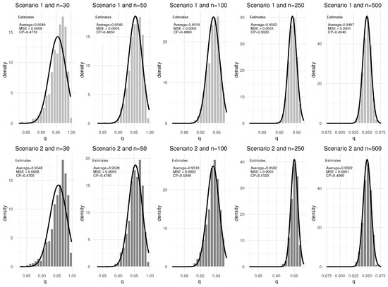
Figure 1. Results from 1000 Monte Carlo replications for the parameter q separated by scenario and sample size with the respective estimated normal curves for 0% censoring.

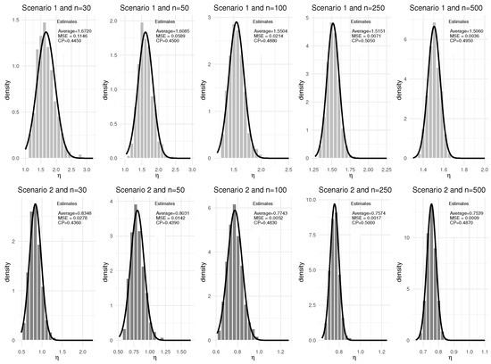
Figure 2. Results from 1000 Monte Carlo replications for the parameter $\eta$ separated by scenario and sample size with the respective estimated normal curves for 0% censoring.

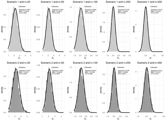
Figure 3. Results from 1000 Monte Carlo replications for the parameter ${\beta }_1$ separated by scenario and sample size with the respective estimated normal curves for 0% censoring.

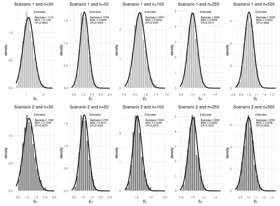
Figure 4. Results from 1000 Monte Carlo replications for the parameter ${\beta }_2$ separated by scenario and sample size with the respective estimated normal curves for 0% censoring.

Analyzing the results of the Figure 1, Figure 2, Figure 3 and Figure 4, it can be seen that the simulations showed that the mean estimates of the parameters studied were close to their true values. The MSEs were close to zero even for smaller sample sizes, and as the sample size becomes larger, the results of the respective analyses converge to their true values, regardless of whether the estimator refers to the baseline distribution (q and $\eta$) or to the estimators related to the covariates (${\beta }_1$ and ${\beta }_2$). The CP’s remained close to the stipulated degree of confidence regardless of the parameter and sample size (the biggest difference is $0.5-0.4360=0.064$ for the $\eta$ parameter in Scenario 2 with sample size equal to 30 and 0% censoring). In addition, it can be inferred that the estimators are asymptotically unbiased. Furthermore, since the increase in sample size leads to lower MSE estimates (lower variance of the estimator), it can be inferred that the estimators are consistent and, from what has been shown, the estimators are asymptotically normal.

The entire evaluation to this point was carried out in the absence of censoring. Therefore, considering the same scenarios and sample sizes, Table 2 shows the estimates (mean of the parameter estimates, MSE, and CP) considering censoring percentages of 0%, 10%, and 30%. These estimates are based on the result of 1000 Monte Carlo replications.

Table 2. Average estimates, MSE, and coverage probability (CP) for the PLSM-DW parameters considering the simulation scenarios and different sample sizes and censoring percentages.

n	Scen.	Cens. Perc.	q			$\mathit{\eta }$			${\mathit{\beta }}_1$			${\mathit{\beta }}_2$
			Average	MSE	CP	Average	MSE	CP	Average	MSE	CP	Average	MSE	CP
30	$S_1$	0%	0.9549	0.0008	0.4710	1.6720	0.1146	0.4450	2.1967	0.3592	0.4650	1.1116	0.1102	0.4660
	$S_2$		0.9548	0.0008	0.4700	0.8348	0.0278	0.4360	2.1919	0.3417	0.4580	1.1096	0.1044	0.4670
	$S_1$	10%	0.9531	0.0009	0.4910	1.6805	0.1316	0.4550	2.1873	0.4327	0.4580	1.1102	0.1385	0.4740
	$S_2$		0.9548	0.0008	0.4800	0.8468	0.0345	0.4420	2.2406	0.4215	0.4700	1.0937	0.0984	0.4550
	$S_1$	30%	0.9525	0.0013	0.4690	1.7631	0.2399	0.4190	2.1337	0.4754	0.4740	1.0854	0.1533	0.4580
	$S_2$		0.9530	0.0010	0.4550	0.8463	0.0430	0.4250	2.2026	0.4496	0.4650	1.1266	0.2111	0.4820
50	$S_1$	0%	0.9540	0.0005	0.4850	1.6085	0.0589	0.4500	2.1364	0.2219	0.4780	1.0789	0.0629	0.4550
	$S_2$		0.9539	0.0005	0.4780	0.8031	0.0142	0.4390	2.1285	0.2066	0.4690	1.0781	0.0617	0.4520
	$S_1$	10%	0.9534	0.0006	0.4740	1.6253	0.0784	0.4350	2.1543	0.2522	0.4440	1.0635	0.0630	0.4980
	$S_2$		0.9536	0.0005	0.4800	0.8104	0.0150	0.4500	2.1180	0.1898	0.4830	1.0263	0.0552	0.5060
	$S_1$	30%	0.9538	0.0007	0.4550	1.6511	0.1005	0.4150	2.1014	0.2798	0.4490	1.0477	0.0717	0.4460
	$S_2$		0.9542	0.0006	0.4580	0.7920	0.0208	0.4950	2.1823	0.2808	0.4690	1.0798	0.0818	0.4850
100	$S_1$	0%	0.9519	0.0002	0.4890	1.5504	0.0214	0.4880	2.0666	0.0784	0.4980	1.0357	0.0252	0.5000
	$S_2$		0.9518	0.0002	0.5040	0.7743	0.0052	0.4830	2.0631	0.0766	0.4980	1.0345	0.0246	0.4970
	$S_1$	10%	0.9505	0.0003	0.5000	1.5460	0.0244	0.4680	2.0348	0.0942	0.4510	1.0247	0.0236	0.4770
	$S_2$		0.9507	0.0003	0.4930	0.7824	0.0064	0.4690	2.0296	0.0852	0.4960	1.0186	0.0215	0.4930
	$S_1$	30%	0.9530	0.0003	0.4910	1.5711	0.0382	0.4860	2.0271	0.1182	0.4730	1.0045	0.0269	0.4390
	$S_2$		0.9510	0.0003	0.4870	0.7722	0.0080	0.4880	2.0587	0.0970	0.4940	1.0336	0.0290	0.4890
250	$S_1$	0%	0.9502	0.0001	0.5020	1.5151	0.0071	0.5050	2.0146	0.0300	0.5050	1.0068	0.0068	0.5310
	$S_2$		0.9502	0.0001	0.5120	0.7574	0.0017	0.5000	2.0146	0.0288	0.5220	1.0068	0.0066	0.5370
	$S_1$	10%	0.9508	0.0001	0.5080	1.5228	0.0086	0.4980	2.0112	0.0301	0.5200	1.0039	0.0088	0.4720
	$S_2$		0.9499	0.0001	0.5070	0.7636	0.0022	0.4740	1.9993	0.0319	0.4740	1.0013	0.0074	0.4940
	$S_1$	30%	0.9518	0.0001	0.5010	1.5273	0.0120	0.4920	1.9853	0.0386	0.4860	0.9897	0.0114	0.4510
	$S_2$		0.9513	0.0001	0.5090	0.7513	0.0029	0.4890	2.0446	0.0387	0.4920	1.0233	0.0102	0.4830
500	$S_1$	0%	0.9497	0.0001	0.4940	1.5060	0.0036	0.4950	2.0016	0.0145	0.4910	1.0039	0.0034	0.4880
	$S_2$		0.9502	0.0001	0.4900	0.7539	0.0009	0.4870	2.0113	0.0147	0.4700	1.0050	0.0036	0.5030
	$S_1$	10%	0.9510	0.0001	0.4950	1.5124	0.0041	0.4960	2.0046	0.0152	0.5160	1.0006	0.0041	0.5160
	$S_2$		0.9505	0.0001	0.5070	0.7592	0.0011	0.4950	2.0096	0.0143	0.5080	1.0033	0.0040	0.4830
	$S_1$	30%	0.9523	0.0001	0.4840	1.5185	0.0059	0.5140	1.9775	0.0198	0.4810	0.9830	0.0057	0.4580
	$S_2$		0.9509	0.0001	0.5140	0.7483	0.0014	0.5040	2.0185	0.0179	0.5030	1.0148	0.0047	0.5160

It can be seen that the results in the presence of censoring are similar to that of the estimators in the absence of censoring, a fact corroborated by the estimates shown in Table 2. Considering the situation with more censoring, i.e., a larger sample size (n = 500) and a higher censoring percentage (30%), the biggest difference between the estimate and the true value of the parameter is 2.000 − 1.9775 = 0.0225 and the largest value of the MSE is 0.01980 (both referring to parameter ${\beta }_1$ in Scenario 1), and the largest difference between the CP and the adopted degree of confidence is 0.5000 − 0.4580 = 0.0420 (referring to parameter ${\beta }_2$ in Scenario 1).

Based on the results of the simulations and the similarity of the results in the absence and presence of censoring, the asymptotic normality of the estimators was met. Therefore, the construction of confidence intervals approximated by a Normal distribution for the parameters of the baseline distribution, as well as for the parameters associated with the covariates, is valid and can be used for interval estimation of the model parameters. As a result, hypothesis tests approximated by a Normal distribution to check the significance of the covariate can also be used in applications.

4. Application

This section presents an application of the PLSM-WD to a dataset obtained from the book [12] and refers to the survival time in weeks of 30 patients with acute myeloid leukemia (AML). The database presents two possible prognostic factors (age and cellularity status). However, similarly to [10], this illustration only considers the covariate age in a dichotomous form:

$$\begin{array}{ccc}\hfill z& =& \left\{\begin{array}{c}1,\mathrm{if} \mathrm{the} \mathrm{patient} \mathrm{is} 50 \mathrm{years} \mathrm{old} \mathrm{or} \mathrm{older}.\hfill \\ 0,\mathrm{otherwise}.\hfill \end{array}\right.\hfill \end{array}$$

The application data are presented in Table 3.

Table 3. Survival time of 30 AML patients.

Survival Time	z	Survival Time	z
18	0	8	1
9	0	2	1
28+	0	26+	1
31	0	10	1
39+	0	4	1
19+	0	3	1
45+	0	4	1
6	0	18	1
8	0	8	1
15	0	3	1
23	0	14	1
28+	0	3	1
7	0	13	1
12	1	13	1
9	1	35+	1

Note: “+” indicates censored observations. Source: [12].

The data in Table 3 were adjusted by the discrete Weibull proportional log survival model (PLSM-DW). Initially, the assumption of the PLSM-WD was verified, observing the proportionality between the levels of the covariate age. The graphs $t\times R_l\left(t\right)$, $l=0,1$, and $R_0\left(t\right)\times R_1\left(t\right)$ and the p-value of hypothesis test (16) are presented in Figure 5.

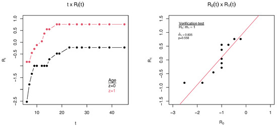
Figure 5. Verification of assumption of proportional log survival for the covariate age.

Through the results of the test presented in Figure 5 it is noted that the assumption of proportional log survival was not rejected (considering a significance level of 5%). The graph $R_0\left(t\right)\times R_1\left(t\right)$ corroborates such a statement since the points formed by the coordinates are close to the adjusted regression line. In addition, the graph $t\times R_l\left(t\right)$, $l=0,1$, also confirms the statement that the proportional log survival assumption is valid since the log-log values of the survival function of the different categories are approximately parallel to each other.

The parameter estimates for the PLSM-WD, taking into account the age covariate, are presented in Table 4.

Table 4. PLSM-DW parameter estimates.

Variable	Parameters	Estimate	Standard Error	CI (95%)	p-Value
Age a	q	0.9881	0.0084	[0.9528; 0.9971]	-
	$\eta$	1.2611	0.1962	[0.8545; 1.8611]	-
	$\beta$	1.1484	0.4383	[0.2894; 2.0074]	0.0088

^a Reference level: The patient is less than 50 years old ($z=0$).

Through the estimates in Table 4, an interpretation can be obtained regarding the odds of survival for the different categories of the age covariate. Since $\exp \left\{\beta \right\}$ represents the ratio of the log survival of the different groups, constant over time, assuming the group of patients that is 50 years or older ($z=1$). In this context, the log survival of a patient who is 50 years or older is $\exp \left\{1.1484\right\}=3.153$ times the log survival of patients younger than 50 years. This result implies that the survival of a patient who is 50 years or older is lower than the survival of a patient who is less than 50 years old (since the logarithm of the survival function is negative).

For diagnostic analysis of the model, by way of comparison, a discrete Weibull proportional odds hazard model (POHM-WD) presented by [9] and a discrete Weibull proportional odds survival model (POSM-WD) presented by [10] were fitted taking into account the data in Table 3.

The survival functions of the POHM-WD and POSM-WD are, respectively, given by the following:

$$S_{POHM-WD}\left(t\right|\mathit{z})=\prod _{k=0}^t\left[{\displaystyle \frac{1-h_0\left(k\right)}{1+(\exp \left\{{\mathit{z}}^{\prime }\mathit{\beta }\right\}-1)h_0\left(k\right)}}\right],$$

(22)

and

$$S_{POSM-WD}\left(t\right|\mathit{z})={\displaystyle \frac{\exp \left\{{\mathit{z}}^{\prime }\mathit{\beta }\right\}{S}_0\left(t\right)}{1+(\exp \left\{{\mathit{z}}^{\prime }\mathit{\beta }\right\}-1)S_0\left(t\right)}}.$$

(23)

where $h_0\left(t\right)={\displaystyle \frac{q^{t^{\eta }}-q^{{(t+1)}^{\eta }}}{q^{t^{\eta }}}}$ and $S_0\left(t\right)=q^{{(t+1)}^{\eta }}$ are, respectively, the hazard and survival functions of DW distribution.

In addition, the maximum errors of the survival function estimates were calculated for the three models considered (Table 5). This error, $ϵ$, is based on the maximum difference between the survival estimates of the models, $\widehat{S}\left(t\right)$, and the empirical Kaplan–Meier (KM) estimates [22]. The maximum error $ϵ$ is defined as follows [23]:

$$ϵ=max|\widehat{S}\left(t\right)-{\widehat{S}}_{KM}\left(t\right)|.$$

(24)

Table 5. Maximum errors from model estimation (AML data).

Covariate Level	${\mathit{ϵ}}_{\mathit{PLSM}-\mathit{WD}}$	${\mathit{ϵ}}_{\mathit{POHM}-\mathit{WD}}$	${\mathit{ϵ}}_{\mathit{POSM}-\mathit{WD}}$
$Z=0$	0.11122	0.11297	0.16937
$Z=1$	0.14214	0.14049	0.11118

Figure 6 shows the fits of the PLSM-DW, POHM-WD and POSM-WD.

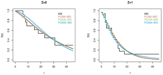
Figure 6. Models fit to leukemia data by level of the age covariate.

Note that, through Table 5 and Figure 6, the three models designed for discrete time-to-event data (PLSM-DW, POHM-DW and POSM-DW) presented a good fit to the data, with the estimates of the survival function of these models always being close to the empirical estimates. It is interesting to note that the PLSM-WD and POHM-WD estimates were practically the same. However, even though the results were similar, the PLSM has the advantage of having a simple closed-form equation for the survival function, which is not the case in the POHM.

5. Conclusions

The aim of this work was to propose a proportional log survival model (PLSM) as an alternative to the proportional odds hazard model [9] and proportional odds survival model [10]. The PLSM is equivalent to the proportional hazards (PH) model when the variable is continuous, but this equivalence does not apply in cases where the variable is discrete. Thus, the PLSM can be seen as a discrete alternative to the PH model.

This paper presented the formulation of the PLSM, as well as the procedures for verifying its assumption. Although the PLSM can be applied to any discrete distribution as a baseline distribution, this work focused on the discrete Weibull distribution (WD), resulting in the discrete Weibull proportional log survival model (PLSM-DW). The parameters of the PLSM-DW were inferred using the maximum likelihood method, and computational optimization methods were applied to obtain the estimates.

A simulation study was carried out using R version 4.3.3 to evaluate the bias, the mean square error of the estimates, and the coverage probability of the proposed asymptotic confidence intervals. These simulations are considered two scenarios. The results showed that the estimators were consistent and asymptotically normal.

The PLSM-DW was illustrated using data on the survival time of patients with leukemia and showed a good fit for the application data, demonstrating that it is a viable alternative for modeling discrete survival data.

For future works, new studies could be conducted to verify the behavior of the PLSM with different discrete baseline distributions and other censoring mechanisms, such as left and interval censoring, as well as the inclusion of time-dependent covariates.

References

- Cox, D.R. Regression models and life-tables. J. R. Stat. Soc. Ser. B (Methodol.) 1972, 34, 187–202. [Google Scholar] [CrossRef]
- Caroni, C. Regression models for lifetime data: An overview. Stats 2022, 5, 1294–1304. [Google Scholar] [CrossRef]
- Gupta, R.C.; Gupta, R.D. Proportional reversed hazard rate model and its applications. J. Stat. Plan. Inf. 2007, 137, 3525–3536. [Google Scholar] [CrossRef]
- Bennett, S. Analysis of survival data by the proportional odds model. Stat. Med. 1983, 2, 273–277. [Google Scholar] [CrossRef] [PubMed]
- Oakes, D.; Dasu, T. Inference for the proportional mean residual life model. Inst. Math. Stat. Lect. Notes 2003, 43, 105–116. [Google Scholar]
- Shrahili, M.; Albabtain, A.A.; Kayid, M.; Kaabi, Z. Stochastic aspects of proportional vitalities model. Mathematics 2020, 8, 1823. [Google Scholar] [CrossRef]
- Asadi, M.; Berred, A. Properties and estimation of the mean past lifetime. Statistics 2012, 46, 405–417. [Google Scholar] [CrossRef]
- Bandos, H. Regression on Median Residual Life Function for Censored Survival Data. Ph.D. Thesis, University of Pittsburgh, Pittsburgh, PA, USA, 2007. [Google Scholar]
- Vieira, M.G.; Cardial, M.R.P.; Matsushita, R.; Nakano, E.Y. Proportional odds hazard model for discrete time-to-event data. Axioms 2023, 12, 1102. [Google Scholar] [CrossRef]
- Cardial, M.R.P.; Cobre, J.; Nakano, E.Y. A discrete Weibull proportional odds survival model. J. Appl. Stat. 2025, 52, 429–447. [Google Scholar] [CrossRef] [PubMed]
- Nakagawa, T.; Osaki, S. The discrete Weibull distribution. IEEE Trans. Reliab. 1975, 24, 300–301. [Google Scholar] [CrossRef]
- Lee, E.T.; Wang, J. Statistical Methods for Survival Data Analysis; John Wiley & Sons: Hoboken, NJ, USA, 2003. [Google Scholar]
- Tutz, G.; Schmid, M. Modeling Discrete Time-to-Event Data; Springer: New York, NY, USA, 2016. [Google Scholar]
- Lehmann, E.L.; Casella, G. Theory of Point Estimation; Springer Science & Business Media: New York, NY, USA, 2006. [Google Scholar]
- Para, B.A.; Jan, T.R. Discrete version of log-logistic distribution and its applications in genetics. Int. J. Mod. Math. Sci. 2016, 14, 407–422. [Google Scholar]
- Cardial, M.R.P.; Fachini-Gomes, J.B.; Nakano, E.Y. Exponentiated discrete Weibull distribution for censored data. Braz. J. Biom. 2020, 38, 35–56. [Google Scholar]
- Krishna, H.; Pundir, P.S. Discrete Burr and discrete Pareto distributions. Stat. Methodol. 2009, 6, 177–188. [Google Scholar] [CrossRef]
- Chakraborty, S. Generating discrete analogues of continuous probability distributions—A survey of methods and constructions. J. Stat. Distrib. Appl. 2015, 2, 1–30. [Google Scholar] [CrossRef]
- Jayakumar, K.; Babu, M.G. Discrete Weibull geometric distribution and its properties. Commun.-Stat.-Theory Methods 2018, 47, 1767–1783. [Google Scholar] [CrossRef]
- R Core Team. R: A Language and Environment for Statistical Computing; R Foundation for Statistical Computing: Vienna, Austria, 2024; Available online: https://www.R-project.org/ (accessed on 20 January 2025).
- Brunello, G.H.V.; Nakano, E.Y. A Bayesian Measure of Model Accuracy. Entropy 2024, 26, 510. [Google Scholar] [CrossRef] [PubMed]
- Kaplan, E.L.; Meier, P. Nonparametric estimation from incomplete observations. J. Am. Stat. Assoc. 1958, 53, 457–481. [Google Scholar] [CrossRef]
- Nakano, E.Y.; Carrasco, C.G. Uma avaliação do uso de um modelo contínuo na análise de dados discretos de sobrevivência. Trends Comput. Appl. Math. 2006, 7, 91–100. [Google Scholar] [CrossRef][Green Version]
Disclaimer/Publisher’s Note: The statements, opinions and data contained in all publications are solely those of the individual author(s) and contributor(s) and not of MDPI and/or the editor(s). MDPI and/or the editor(s) disclaim responsibility for any injury to people or property resulting from any ideas, methods, instructions or products referred to in the content. |
© 2025 by the authors. Licensee MDPI, Basel, Switzerland. This article is an open access article distributed under the terms and conditions of the Creative Commons Attribution (CC BY) license (https://creativecommons.org/licenses/by/4.0/).