Calculation and Analysis of Petri Net Reachability Graphs by a Think-Globally-Act-Locally Method

Abstract

A think-globally-act-locally (TGAL) technique is proven to be an effective method to address the state explosion issue for complex discrete event systems modeled with Petri nets. This paper introduces a TGAL-based method for computing and analyzing the reachability graph (RG) of Petri net models. Given a net system, the TGAL technique strategically introduces a global idle place (GIP) to iteratively generate its RG by updating the token count. At each step, the reachable markings (RMs) and legal markings (LMs) obtained by the previous iterations are considered to calculate the corresponding states of the current step. According to the enforced control requirement, a system state is required to be computed and classified only once during an iterative process. This method only calculates the necessary number of RMs and reduces computational redundancy, which minimizes the computational cost. Four typical Petri net models from existing studies are employed to demonstrate the method.

1. Introduction

Discrete event systems (DESs) are event-driven systems with discrete-states that evolve with the occurrences of discrete events. For DESs, supervisory control techniques are employed to restrict their behavior to implement the various control requirements [1,2,3,4]. As a graphical tool for the effective modeling and investigating of complex systems, Petri nets play a vital role in the field of supervisory control of DESs. A large number of supervisory control policies have been proposed for DESs modeled with Petri nets [5,6,7,8,9,10].

In the context of Petri nets, supervisory control techniques are categorized into two groups: structural analysis [11,12] and reachability graph (RG) analysis [13]. In general, structural analysis methods are usually available for certain Petri net models with special structures, namely, siphons and resource circuits [12]. Unlike structural analysis methods, an RG analysis approach can enforce the desired control requirement for a generalized net model. Nevertheless, an RG analysis method has to enumerate and classify all reachable markings (RMs) of a net system, which grow exponentially with the scale of the system [14]. It limits the application of RG analysis methods to complex systems. Consequently, deciding how to completely calculate the RG of large-scale systems becomes the key to the effective utilization of these methods [15,16,17].

Generally, the RG calculation depends on three factors: next-state function, iterative strategies, and variable ordering. In [18], a symbolic method is developed to implicitly generate the RMs of bounded Petri net systems. By utilizing a binary decision diagram (BDD), this method compresses a large number of RMs into encoded data with small structures and accurately manipulates RMs. However, the effectiveness of this method is highly dependent on the ordering of variables. Furthermore, Chen et al. introduce a BDD-based technique to generate the RG of a net system [19]. Given a deadlock-free control specification for a net system, its RMs are classified into two groups: legal markings (LMs) and illegal markings (ILMs). They first compute the sets of LMs and first-met bad markings (FBMs), where an FBM is an ILM reached by triggering a transition at an LM. Then, two minimal covering sets of LMs and FBMs are obtained to compute an optimal supervisor. As a result, this method is more powerful for generating RGs of complex net models than those traditional techniques in [18,20,21].

In order to mitigate the state explosion issue, Ma et al. develop a compact representation of the RG, referred to as a basis RG (BRG) [22]. This method distinguishes between the transitions of a net system as either implicit or explicit, where the subnet induced by implicit transitions needs to be acyclic. By only considering explicit transitions, a set of basis markings is calculated to construct the corresponding BRG, which can efficiently represent all RMs of a net system. In general, the BRG has a small number of nodes and arcs since the number of RMs is much larger than that of basis markings. In [23], an effective methodology is proposed to generate the RMs for a large-sized net system, by using multi-valued decision diagrams (MDDs). This method can generate the RMs concurrently and compactly store the set of RMs. Consequently, it is more efficient than the techniques based on the RG and the BRG.

On the other hand, a think-globally-act-locally (TGAL) technique is developed by Uzam et al. in [24]. This method strategically designs a global idle place (GIP) to enumerate the RG of a net system iteratively. The introduction of the GIP will not change any basic property of the net model. Due to the limitation of the available resources in the GIP, the corresponding net model has a small number of RMs at each iteration. It is obvious that this method mitigates the state explosion issue for a complex system. Furthermore, in order to construct monitors with weighted arcs, a think-globally-act-locally approach with weighted arcs (TGALW) is proposed in [25]. They transform a Petri net model into a special form, which has the isomorphic RG to the original net system. In theory, this method has the same complexity as the TGAL approach in terms of the RG computation.

Similarly, a number of TGAL-based methods for optimal control of a net system are proposed in [26,27]. At each iteration, these methods generate and analyze the RG of the corresponding net system. A set of optimal control places is calculated during an iterative process. Compared with the previous TGAL [24] and TGALW [25] approaches, these methods guarantee the resulting net system with more RMs. Nevertheless, the existing TGAL-based approaches suffer from the problem of repeated calculation. First, the computation of previously derived RMs is reiterated in subsequent iterations. Then, the analysis of previously classified RMs is reiterated in subsequent iterations. As a consequence, these methods cause a huge waste of computing power.

This paper introduces a TGAL-based approach to compute and analyze the RG of a Petri net system. Compared with the previous TGAL-based methods [24,25,26,27], the proposed method calculates and analyzes a minimized number of RMs. This means that this method is more advantageous in terms of computational cost. Moreover, compared with the approaches in [24,25,26,27], the proposed method takes less time to calculate the RG of a net model, i.e., its performance is better in terms of computation time. Ultimately, the primary contributions of this study are presented in the following.

(1)

A TGAL-based approach is developed to compute the RG of a net system. At each step, by considering the previously computed states, the partial RMs of the corresponding net model are directly obtained. Then, the enabled transitions of the obtained states are analyzed to generate the remaining RMs of the corresponding net model. It is obvious that all RMs calculated at the current step are new states. Finally, its complete RG is derived through iterations. In this case, all nodes of the RG are required to be enumerated only once during an iteration.

(2)

A TGAL-based method is proposed to explore the RG of a net system. The TGAL method only updates the token count in the GIP at each step, which will not change the legal performance of a state. The previously obtained LMs are still legal for subsequent iterations, i.e., analyzing all RMs at the next step is unnecessary. At each iteration, according to the previously computed LMs, the newly generated states are classified. Finally, the complete RG of the net system is analyzed iteratively.

The remainder of this paper is structured as follows. In Section 2, a TGAL-based policy is provided to generate and analyze the RG of a Petri net system. Section 3 presents several net systems to demonstrate the proposed technique. Ultimately, Section 4 provides a summary of this work and outlines potential directions for future research. Appendix A provides a descriptionof Petri nets [28] and an analysis of the RG [27].

2. Computation and Analysis of an RG

This section proposes a TGAL-based method to generate and classify the RMs of a Petri net model. Given a net system $(N,M_0)$, the TGAL approach introduces a GIP $\widehat{p}$ into the net system $(N,M_0)$, where $N=(P^0\cup P_A\cup P_R$, T, F, $W)$. The net system with $\widehat{p}$ is represented as $(N^{\prime },M_0^b)$, where $N^{\prime }=(P^0\cup P_A\cup P_R\cup \left\{\widehat{p}\right\},T,F,W)$, $M_0^b\left(\widehat{p}\right)=b$ ($1\le b\le {\sum }_{p\in P^0}{M}_0\left(p\right)$), and for all $p\in P^0\cup P_A\cup P_R$, $M_0^b\left(p\right)=M_0\left(p\right)$. Initially, the GIP $\widehat{p}$ has one token, i.e., a net $(N^{\prime },M_0^1)$ is generated to calculate its RG. Next, one token adds to $\widehat{p}$ to analyze a net model $(N^{\prime },M_0^2)$. This iterative process continues until the number of RMs does not change by increasing tokens in $\widehat{p}$. In such a case, all RMs of the net system $(N,M_0)$ are enumerated iteratively. Suppose that M and $M^{\prime }$ are RMs for $(N^{\prime },M_0^a)$ and $(N^{\prime },M_0^b)$, respectively, where $a\ne b$. For markings M and $M^{\prime }$, the following definition is obtained.

Definition 1.

Let $(N^{\prime },M_0^a)$ and $(N^{\prime },M_0^b)$ be two net systems, and M and $M^{\prime }$ be two RMs for $(N^{\prime },M_0^a)$ and $(N^{\prime },M_0^b)$, respectively, where $a\ne b$. Markings M and $M^{\prime }$ are referred to as N-identical if for all $p\in P^0\cup P_A\cup P_R$, $M\left(p\right)=M^{\prime }\left(p\right)$ holds, which is represented as $M{=}_N{M}^{\prime }$.

By Definition 1, $M\left(\widehat{p}\right)\ne M^{\prime }\left(\widehat{p}\right)$ and $M\left(p\right)=M^{\prime }\left(p\right)$ are obtained if M and $M^{\prime }$ are N-identical markings, where $p\in P^0\cup P_A\cup P_R$. Obviously, markings M and $M^{\prime }$ signify the same state of a system. In such a case, M and $M^{\prime }$ are required to be computed only once during an iteration. If $M^{\prime }$ has already been obtained, M is generated by only changing the token count in $\widehat{p}$. In this case, the partial RMs of the net $(N^{\prime },M_0^b)$ are yielded directly if all markings of the net $(N^{\prime },M_0^{b-1})$ are known, where $2\le b\le {\sum }_{p\in P^0}{M}_0\left(p\right)$.

Example 1.

We assume $M=p_4+p_7$ and $M^{\prime }=p_4+p_7+\widehat{p}$ to be two RMs obtained during an iteration. By Definition 1, M and $M^{\prime }$ are N-identical markings due to $M{=}_N{M}^{\prime }$. In this case, $M^{\prime }$ can be computed by only increasing the token count in $\widehat{p}$ for M. Markings M and $M^{\prime }$ correspond to the same state of a system.

Then, the RMs of $(N^{\prime },M_0^{b-1})$ are analyzed to further calculate the RMs of the next step, namely, a net $(N^{\prime },M_0^b)$, where $2\le b\le {\sum }_{p\in P^0}{M}_0\left(p\right)$. Suppose that M is an RM that is computed in the $(b-1)$-th iteration and the enabled transition at M is t. In the b-th iteration, transition t may be enabled at $M^{\prime }$, where M and $M^{\prime }$ denote N-identical markings and $M^{\prime }\left(\widehat{p}\right)=M\left(\widehat{p}\right)+1$. In this case, firing t at $M^{\prime }$ yields an RM, which must be a new state of the system obtained at the b-th step. Consequently, the newly enabled transitions are considered to compute a set of RMs in the b-th iteration. We use ${\mathcal{E}}_M$ to represent the set of transitions enabled at marking M, defined as ${\mathcal{E}}_M=\{t\in T|M[t⟩\}$. Assume that $R(N^{\prime },M_0^{b-1})$ is the set of RMs for $(N^{\prime },M_0^{b-1})$ and ${\mathcal{E}}_M$ represents the set of enabled transitions, where $M\in R(N^{\prime },M_0^{b-1})$. Algorithm 1 presents a TGAL-based approach to generate the RMs of a net system $(N^{\prime },M_0^b)$.

Algorithm 1 Computation of RMs for a net model $(N^{\prime },M_0^b)$

Input:  A net model $(N^{\prime },M_0^b)$, a set of RMs $R(N^{\prime },M_0^{b-1})$, and a set of enabled transitions ${\mathcal{E}}_M$, where $M\in R(N^{\prime },M_0^{b-1})$ and $2\le b\le {\sum }_{p\in P^0}{M}_0\left(p\right)$. Output:  A set of RMs $R(N^{\prime },M_0^b)$. 1: for each {$M\in R(N^{\prime },M_0^{b-1})$} do 2:        $M^{\prime }:=M$. 3:        $M^{\prime }\left(\widehat{p}\right):=M\left(\widehat{p}\right)+1$. 4:        $R(N^{\prime },M_0^b):=R(N^{\prime },M_0^b)\cup \left\{M^{\prime }\right\}$. 5:        Compute the set of enabled transitions ${\mathcal{E}}_{M^{\prime }}$. 6:        ${\mathcal{E}}_{M^{\prime }}^{\prime }:={\mathcal{E}}_{M^{\prime }}\setminus {\mathcal{E}}_M$. 7: $\mathcal{M}:=\varnothing$. 8: for each {$M\in R(N^{\prime },M_0^b)$} do 9:        for each {$t\in {\mathcal{E}}_M^{\prime }$} do 10:            $M^{\prime }:=M+\left[N^{\prime }\right](·,t)$. 11:            if {$M^{\prime }\notin R(N^{\prime },M_0^b)$} do 12:               $\mathcal{M}:=\mathcal{M}\cup \left\{M^{\prime }\right\}$. 13: $R(N^{\prime },M_0^b):=R(N^{\prime },M_0^b)\cup \mathcal{M}$. 14: for each {$M\in \mathcal{M}$} do 15:        Compute the set of enabled transitions ${\mathcal{E}}_M$. 16:        for each {$t\in {\mathcal{E}}_M$} do 17:            $M^{\prime }:=M+\left[N^{\prime }\right](·,t)$. 18:            if {$M^{\prime }\notin R(N^{\prime },M_0^b)$} do 19:               $R(N^{\prime },M_0^b):=R(N^{\prime },M_0^b)\cup \left\{M^{\prime }\right\}$. 20: Output $R(N^{\prime },M_0^b)$. 21: End.

In Algorithm 1, a part of RMs for the net $(N^{\prime },M_0^b)$ ($2\le b\le {\sum }_{p\in P^0}{M}_0\left(p\right)$) can be directly obtained by considering the markings in $R(N^{\prime },M_0^{b-1})$, that is, the token count in the GIP $\widehat{p}$ is increased by one for a marking in $R(N^{\prime },M_0^{b-1})$. Then, the remaining RMs of $(N^{\prime },M_0^b)$ are computed by utilizing the previously generated markings. Finally, we enumerate all RMs in $R(N^{\prime },M_0^b)$.

Example 2.

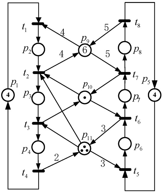
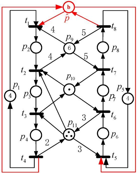
A net system depicted in Figure 1 is considered. By introducing a GIP $\widehat{p}$, the corresponding net $(N^{\prime },M_0^b)$ shown in Figure 2 is constructed, where b represents the token count in $\widehat{p}$. When $b=1$, we derive a net system $(N^{\prime },M_0^1)$. There is a marking $M=3p_1+p_2+4p_5+2p_9+p_{10}+3p_{11}$ for $(N^{\prime },M_0^1)$. At M, we have the set of enabled transitions ${\mathcal{E}}_M=\left\{t_2\right\}$. By Algorithm 1, an RM $M^{\prime }=3p_1+p_2+4p_5+2p_9+p_{10}+3p_{11}+\widehat{p}$ is generated directly for a net system $(N^{\prime },M_0^2)$ (i.e., $b=2$). Similarly, at $M^{\prime }$, ${\mathcal{E}}_{M^{\prime }}=\{t_2$, $t_5\}$ is calculated. We have ${\mathcal{E}}_{M^{\prime }}^{\prime }={\mathcal{E}}_{M^{\prime }}\setminus {\mathcal{E}}_M=\left\{t_5\right\}$. It is clear that firing $t_5$ at $M^{\prime }$ generates a new marking $M^{″}=3p_1+p_2+3p_5+p_6+2p_9+p_{10}$. Meanwhile, by analyzing $M^{″}$, an RM $M^{″\prime }=3p_1+p_2+3p_5+p_7+2p_9+3p_{11}$ is obtained for $(N^{\prime },M_0^2)$. Finally, this method enumerates all RMs of $(N^{\prime },M_0^2)$.

Figure 1. A net system from [14].

Figure 2. A net system $(N^{\prime },M_0^b)$.

For an optimal control requirement, the RMs in $R(N^{\prime },M_0^b)$ are required to be classified into LMs and ILMs. We suppose M and $M^{\prime }$ to be two N-identical markings for $(N^{\prime },M_0^a)$ and $(N^{\prime },M_0^b)$, respectively, where $a\ne b$. According to Definition 1, M and $M^{\prime }$ represent the same state of a system. At each iteration, the control requirement of the system will not be changed over time. The legality of marking M is independent of the token count in the GIP $\widehat{p}$. We only need to analyze M for $(N^{\prime },M_0^a)$ to determine whether $M^{\prime }$ is legal or not for $(N^{\prime },M_0^b)$. As a consequence, at each iteration, the sets of LMs and ILMs can be computed by considering the previously partitioned states. The following propositions are obtained.

Proposition 1.

Let M and $M^{\prime }$ be two N-identical markings for $(N^{\prime },M_0^a)$ and $(N^{\prime },M_0^b)$, respectively, where $a\ne b$. Then, M is legal (resp. illegal) for $(N^{\prime },M_0^a)$ if and only if $M^{\prime }$ is an LM (resp. an ILM) for $(N^{\prime },M_0^b)$.

Proof. 

Given a net system $(N,M_0)$, a net model $(N^{\prime },M_0^b)$ is constructed by adding a GIP $\widehat{p}$, where b represents the token count in $\widehat{p}$. We suppose M and $M^{\prime }$ to be N-identical markings for $(N^{\prime },M_0^a)$ and $(N^{\prime },M_0^b)$, respectively, where $a\ne b$. According to Definition 1, M and $M^{\prime }$ denote the same marking $\widehat{M}$ of the net system $(N,M_0)$. Given a control specification, marking $\widehat{M}$ has only two cases: legal and illegal. Compared with $\widehat{M}$, markings M and $M^{\prime }$ have a different number of tokens in $\widehat{p}$. Nevertheless, only changing the token count in $\widehat{p}$ will not lead to the reallocation of the system resources. This means that M and $M^{\prime }$ are LMs (resp. ILMs) for $(N^{\prime },M_0^a)$ and $(N^{\prime },M_0^b)$, respectively, if and only if $\widehat{M}$ is legal (resp. illegal) for $(N,M_0)$. In this case, whether M is legal for $(N^{\prime },M_0^a)$ can be directly determined by checking $M^{\prime }$ for $(N^{\prime },M_0^b)$. That is to say, M is legal (resp. illegal) for $(N^{\prime },M_0^a)$ if and only if $M^{\prime }$ is an LM (resp. an ILM) for $(N^{\prime },M_0^b)$. Finally, the conclusion is true.    □

Proposition 2.

A marking $M^{\prime }$ is legal if there is an LM M such that $M^{\prime }[\sigma ⟩M$ holds, where σ is a transition sequence.

Proof. 

Since M is an LM, there is at least a transition sequence ${\sigma }^{\prime }$ from M to the initial marking $M_0$. Suppose that there is a transition sequence ${\sigma }^{″}$ such that $M^{\prime }[{\sigma }^{″}⟩M$ holds. In such a case, we have $M^{\prime }[{\sigma }^{″}⟩M[{\sigma }^{\prime }⟩M_0$ and $M^{\prime }[\sigma ⟩M_0$, where $\sigma ={\sigma }^{\prime }{\sigma }^{″}$. By the definition of LMs, marking $M^{\prime }$ is legal, which completes the proof.    □

Suppose that $R(N^{\prime },M_0^b)$ is a set of RMs for the net $(N^{\prime },M_0^b)$ and ${\mathcal{M}}_{L_{b-1}}$ is a set of LMs for the net $(N^{\prime },M_0^{b-1})$, where $2\le b\le {\sum }_{p\in P^0}{M}_0\left(p\right)$. According to Propositions 1 and 2, Algorithm 2 is proposed to calculate LMs and ILMs of a net system $(N^{\prime },M_0^b)$.

Algorithm 2 Calculation of LMs and ILMs for a net model $(N^{\prime },M_0^b)$

Input:  A net model $(N^{\prime },M_0^b)$, a set of RMs $R(N^{\prime },M_0^b)$, and a set of LMs ${\mathcal{M}}_{L_{b-1}}$. Output:  A set of LMs ${\mathcal{M}}_{L_b}$ and a set of ILMs ${\mathcal{M}}_{\overline{L_b}}$. 1: for each {$M\in {\mathcal{M}}_{L_{b-1}}$} do 2:        $M^{\prime }:=M$. 3:        $M^{\prime }\left(\widehat{p}\right):=M^{\prime }\left(\widehat{p}\right)+1$. 4:        ${\mathcal{M}}_{L_b}:={\mathcal{M}}_{L_b}\cup \left\{M^{\prime }\right\}$. 5: $\mathcal{M}:=R(N^{\prime },M_0^b)\setminus {\mathcal{M}}_{L_b}$. 6: for each {$M\in \mathcal{M}$} do 7:        if {a marking $M^{\prime }\in R(N^{\prime },M)$ that satisfies $M^{\prime }\in {\mathcal{M}}_{L_b}$} do 8:            ${\mathcal{M}}_{L_b}:={\mathcal{M}}_{L_b}\cup \left\{M\right\}$. 9: ${\mathcal{M}}_{\overline{L_b}}:=R(N^{\prime },M_0^b)\setminus {\mathcal{M}}_{L_b}$. 10: Output ${\mathcal{M}}_{L_b}$ and ${\mathcal{M}}_{\overline{L_b}}$. 11: End.

By considering the states in ${\mathcal{M}}_{L_{b-1}}$, Algorithm 2 first computes a part of the LMs and adds them into the set ${\mathcal{M}}_{L_b}$. Then, $\mathcal{M}:=R(N^{\prime },M_0^b)\setminus {\mathcal{M}}_{L_b}$ is obtained. A marking $M\in \mathcal{M}$ is selected to determine whether it is legal or not, if a marking $M^{\prime }\in {\mathcal{M}}_{L_b}$ that meets $M[\sigma ⟩M^{\prime }$, M is an LM and ${\mathcal{M}}_{L_b}:={\mathcal{M}}_{L_b}\cup \left\{M\right\}$ is obtained, where $\sigma$ is a transition sequence. By analyzing each marking in $\mathcal{M}$, a set of LMs ${\mathcal{M}}_{L_b}$ is figured out from $R(N^{\prime },M_0^b)$. Meanwhile, a set of ILMs for the net $(N^{\prime },M_0^b)$ is computed with ${\mathcal{M}}_{\overline{L_b}}:=R(N^{\prime },M_0^b)\setminus {\mathcal{M}}_{L_b}$.

Example 3.

Continue to consider the net system $(N^{\prime },M_0^b)$ depicted in Figure 2. When $b=1$, a net system $(N^{\prime },M_0^1)$ is obtained, which has an LM $M=3p_1+p_3+4p_5+6p_9+2p_{11}$. By Algorithm 2, $M^{\prime }=3p_1+p_3+4p_5+6p_9+2p_{11}+\widehat{p}$ is an LM for a net system $(N^{\prime },M_0^2)$ (namely, $b=2$). At the same time, marking $M^{″}=2p_1+p_3+p_4+4p_5+6p_9$ is legal since there is transition $t_4$ such that $M^{″}[t_4⟩M^{\prime }$ holds. Finally, this method partitions the RMs for $(N^{\prime },M_0^2)$ into a set of LMs and a set of ILMs.

Finally, a TGAL-based technique is introduced to generate and classify the RMs for a Petri net model, as presented in Algorithm 3.

Algorithm 3 Analysis of RG for a net system

Input:  A net system $(N,M_0)$, where $N=(P^0\cup P_A\cup P_R$, T, F, $W)$. Output:  A set of RMs $R(N,M_0)$, a set of LMs ${\mathcal{M}}_L$, and a set of ILMs ${\mathcal{M}}_{\overline{L}}$. 1: Construct a GIP $\widehat{p}$ with ${}_{ }{}^{ }\widehat{p}_{ }^{•}:=P^{0•}$, ${}_{ }{}^{•}\widehat{p}_{ }^{ }:={}_{ }{}^{•}P_{ }^0$, and $M_0\left(\widehat{p}\right):=b$. /* b denotes the token count in $\widehat{p}$. */ 2: Add the GIP $\widehat{p}$ to the original net $(N,M_0)$, which is defined as $(N^{\prime },M_0^b)$. 3: $b:=1$ and $R(N^{\prime },M_0^1):=\left\{M_0\right\}$. 4: for each {$M\in R(N^{\prime },M_0^1)$} do 5:        Compute the set of enabled transitions ${\mathcal{E}}_M$. 6:        for each {$t\in {\mathcal{E}}_M$} do 7:            $M^{\prime }:=M+\left[N^{\prime }\right](·,t)$. 8:            if {$M^{\prime }\notin R(N^{\prime },M_0^1)$} do 9:               $R(N^{\prime },M_0^1):=R(N^{\prime },M_0^1)\cup \left\{M^{\prime }\right\}$. 10: $R(N,M_0):=R(N,M_0)\cup R(N^{\prime },M_0^1)$. 11: Derive the sets of LMs ${\mathcal{M}}_{L_1}$ and ILMs ${\mathcal{M}}_{\overline{L_1}}$ from $R(N^{\prime },M_0^1)$. 12: ${\mathcal{M}}_L:={\mathcal{M}}_L\cup {\mathcal{M}}_{L_1}$. 13: ${\mathcal{M}}_{\overline{L}}:={\mathcal{M}}_{\overline{L}}\cup {\mathcal{M}}_{\overline{L_1}}$. 14: $b:=b+1$. 15: while {$b\le {\sum }_{p\in P^0}{M}_0\left(p\right)$} do 16:        Obtain the set of RMs $R(N^{\prime },M_0^b)$ by Algorithm 1. 17:        Calculate the set of LMs ${\mathcal{M}}_{L_b}$ and the set of ILMs ${\mathcal{M}}_{\overline{L_b}}$ for $(N^{\prime },M_0^b)$ by Algorithm 2. 18:        ${\mathcal{M}}_L:={\mathcal{M}}_L\cup {\mathcal{M}}_{L_b}$. 19:        ${\mathcal{M}}_{\overline{L}}:={\mathcal{M}}_{\overline{L}}\cup {\mathcal{M}}_{\overline{L_b}}$. 20:        $R(N,M_0):=R(N,M_0)\cup R(N^{\prime },M_0^b)$. 21:        $b++$. 22: Output $R(N,M_0)$, ${\mathcal{M}}_L$, and ${\mathcal{M}}_{\overline{L}}$. 23: End.

Algorithm 3 first constructs a GIP $\widehat{p}$ for a net system $(N,M_0)$ and denotes the corresponding net as $(N^{\prime },M_0^b)$, where b ($1\le b\le {\sum }_{p\in P^0}{M}_0\left(p\right)$) represents the token count in $\widehat{p}$. Initially, the token count in $\widehat{p}$ is one, namely, $b=1$. For a net system $(N^{\prime },M_0^1)$, we calculate the set of RMs $R(N^{\prime },M_0^1)$. According to the control requirement, the markings in $R(N^{\prime },M_0^1)$ are considered to derive a set of LMs ${\mathcal{M}}_{L_1}$ and a set of ILMs ${\mathcal{M}}_{\overline{L_1}}$. Then, one token adds to $\widehat{p}$, i.e., a net $(N^{\prime },M_0^2)$ ($b=2$) is generated. By the markings in $R(N^{\prime },M_0^1)$, Algorithm 1 computes the set of RMs for $(N^{\prime },M_0^2)$. Meanwhile, based on the LMs in ${\mathcal{M}}_{L_1}$, the sets of LMs and ILMs for $(N^{\prime },M_0^2)$ are calculated utilizing Algorithm 2. We terminate this process if the number of RMs does not grow with the increase in the tokens in $\widehat{p}$. Finally, the sets of RMs, LMs, and ILMs for the original net system are obtained iteratively.

Next, the complexity of Algorithm 3 is reviewed. This approach is still necessary to enumerate all of the RMs of a system. It is obvious that the number of RMs increases exponentially as the scale of the net system grows, i.e., the proposed method exhibits exponential complexity in theory. Nevertheless, this method can effectively alleviate the state explosion issue, as only a small number of new RMs are generated at each iteration. Compared with the previous TGAL-based methods [24,25,26,27], it greatly reduces the repeated calculations of a marking, that is, each marking of the system needs to be computed and classified only once. Consequently, it has more advantages in terms of computation time.

Example 4.

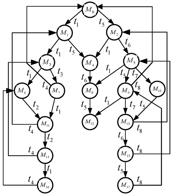
We continue to analyze the net system depicted in Figure 1. By Algorithm 3, a set of RMs is computed iteratively, which contains 18 markings. Then, the RMs are partitioned into LMs and ILMs. Table 1 presents iteration steps, where the first column indicates the iteration count and the second column is the RM count computed at the b-th step. The counts of LMs and ILMs are given in the third and fourth columns, respectively, and the last column signifies the calculation time. Since the net system only has 18 RMs, the computation time of each step is close to zero seconds. Figure 3 shows the obtained RG, where $M_0$, $M_1$, $M_2$, $M_3$, $M_5$, $M_7$, and $M_{10}$ are generated at the first iteration (namely, $b=1$). When $b=2$, $M_4$, $M_6$, $M_8$, $M_9$, $M_{11}$, $M_{13}$, $M_{14}$, and $M_{15}$ are computed. At the third step (i.e., $b=3$), we obtain markings $M_{12}$, $M_{16}$, and $M_{17}$. Table 2 gives the details of RMs in the RG.

Table 1. Iteration steps of the net system depicted in Figure 1.

b	RMs	ILMs	LMs	Time
1	7		7	<0.1 s
2	8	2	6	<0.1 s
3	3	1	2	<0.1 s
total	18	3	15	<0.3 s

Figure 3. RG of the net shown in Figure 1.

Table 2. RMs of the net system shown in Figure 1.

$M_0=4p_1+4p_5+6p_9+p_{10}+3p_{11}$	$M_1=3p_1+p_2+4p_5+2p_9+p_{10}+3p_{11}$
$M_2=4p_1+3p_5+p_6+6p_9+p_{10}$	$M_3=3p_1+p_3+4p_5+6p_9+2p_{11}$
$M_4=3p_1+p_2+3p_5+p_6+2p_9+p_{10}$	$M_5=4p_1+3p_5+p_7+6p_9+3p_{11}$
$M_6=2p_1+p_2+p_3+4p_5+2p_9+2p_{11}$	$M_7=3p_1+p_4+4p_5+6p_9+p_{10}+p_{11}$
$M_8=3p_1+p_2+3p_5+p_7+2p_9+3p_{11}$	$M_9=4p_1+2p_5+p_6+p_7+6p_9$
$M_{10}=4p_1+3p_5+p_8+p_9+p_{10}+3p_{11}$	$M_{11}=2p_1+p_2+p_4+4p_5+2p_9+p_{10}+p_{11}$
$M_{12}=3p_1+p_2+2p_5+p_6+p_7+2p_9$	$M_{13}=4p_1+2p_5+p_6+p_8+p_9+p_{10}$
$M_{14}=2p_1+p_3+p_4+4p_5+6p_9$	$M_{15}=4p_1+2p_5+p_7+p_8+p_9+3p_{11}$
$M_{16}=p_1+p_2+p_3+p_4+4p_5+2p_9$	$M_{17}=4p_1+p_5+p_6+p_7+p_8+p_9$

3. Examples

In this section, we utilize some typical net systems of FMSs to demonstrate the proposed method. We design C++ programs to generate the sets of RMs, LMs, and ILMs for a net model. In this work, all of the computations for these examples were performed on a computer running Windows 11, equipped with an Intel Core 2.8 GHz CPU and 16GB of memory.

First, a net system depicted in Figure 4 is selected, which is from the literature [29].

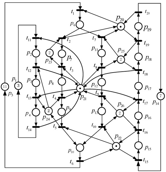
Figure 4. A net system from [29].

This net system contains 26,750 RMs, of which 21,581 and 5169 are LMs and ILMs, respectively. We utilize the proposed technique to compute the RG of this net system. In Table 3, the details of the iteration steps are presented. Table 4 compares the performance of the several algorithms applied for this net system. From the perspective of space complexity analysis, compared with the approaches in [24,26], our method only computes 19.5% and 18.6% of the total number of RMs and LMs, respectively. This means that this method does not involve the repeated enumeration and analysis of a system state. From the perspective of time complexity analysis, compared with the techniques in [24,26], this method can save 70.0% and 24.7% of the time cost, respectively. That is to say, it performs better than the methods in [24,26].

Table 3. Iteration steps of the net system depicted in Figure 4.

b	RMs	ILMs	LMs	Time
1	17		17	<0.1 s
2	115		115	<0.1 s
3	505	5	500	<0.1 s
4	1520	48	1472	1.4 s
5	3303	217	3086	8.1 s
6	5289	601	4688	25.3 s
7	6241	1106	5135	54.2 s
8	5322	1363	3959	89.6 s
9	3128	1120	2008	95.2 s
10	1128	583	545	58.5 s
11	182	126	56	36.2 s
total	26,570	5169	21,581	<368.8 s

Table 4. Performance comparison of different methods.

Parameters	[24]	[26]	Proposed Method
No. RMs	137,212	137,212	26,750
No. LMs	116,024	116,024	21,581
Time	<489.7 s	<1230.6 s	<368.8 s

Then, a net system from [25], depicted in Figure 5, is employed to demonstrate this technique. This net system has 54,869 RMs, including 51,506 LMs and 3363 ILMs. Table 5 presents the iteration steps of the proposed method. Table 6 provides a comparative analysis of the performance of different techniques for this net system. In terms of space complexity, compared with the methods in [24,26], the number of RMs and LMs are reduced by 296,657 and 277,205, respectively. In terms of time complexity, it only takes 9.0% of the computation time used by the approach in [26]. Meanwhile, this method saves 177.0 s to generate its RG compared with the approach in [24].

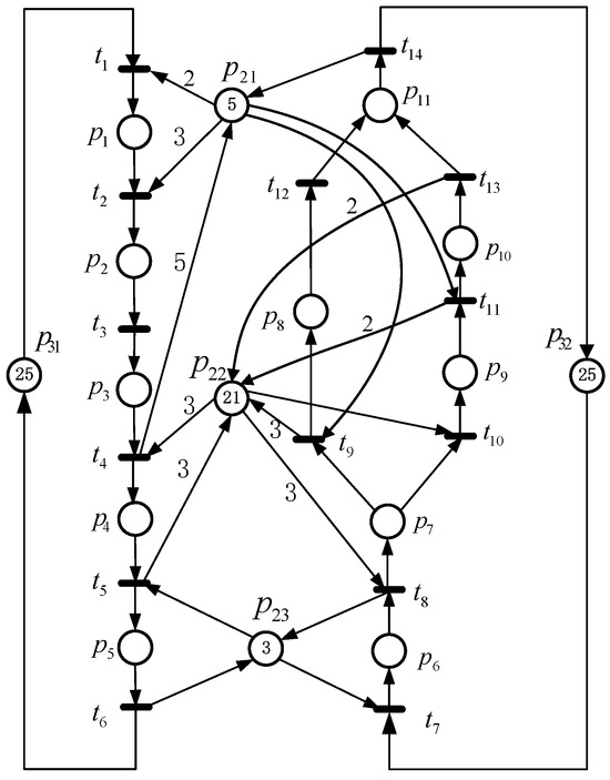
Figure 5. A net system from [25].

Table 5. Iteration steps of the net system depicted in Figure 5.

b	RMs	ILMs	LMs	Time
1	12		12	<0.1 s
2	55	1	54	<0.1 s
3	194	8	186	<0.1 s
4	545	30	515	<0.1 s
5	1276	80	1196	1.5 s
6	2573	174	2399	2.4 s
7	4522	314	4208	4.4 s
8	6905	489	6416	14.8 s
9	9066	650	8416	32.7 s
10	10,028	713	9315	75.6 s
11	9022	577	8445	115.3 s
12	6326	285	6041	117.2 s
13	3202	42	3160	125.9 s
14	1017		1017	127.3 s
15	126		126	119.6 s
total	54,869	3363	51,506	<737.1 s

Table 6. Performance comparison of different methods.

Parameters	[24]	[26]	Proposed Method
No. RMs	351,526	351,526	54,869
No. LMs	328,711	328,711	51,506
Time	<914.1 s	<8174.9 s	<737.1 s

We continue to use the net system shown in Figure 6 to test the proposed approach, which has 68,531 RMs. According to the deadlock-free control specification, the numbers of LMs and ILMs are 66,400 and 2131, respectively. By introducing a GIP, the proposed method generates its RG iteratively, and Table 7 presents the iteration steps. Table 8 gives a comparative analysis of the performance of different algorithms applied to this net system. Similarly, the space complexity of this method is lower, i.e., the proposed method only requires calculating 18.6% of the RMs and 18.5% of the LMs compared with the techniques in [24,26]. In terms of time complexity, compared with the approaches in [24,26], it saves 8,792.3 s and 103.8 s, respectively. Consequently, the performance of those in [24,26] is poor compared with the proposed method.

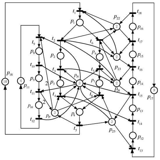
Figure 6. A net system from [25].

Table 7. Iteration steps of the net system depicted in Figure 6.

b	RMs	ILMs	LMs	Time
1	15		15	<0.1 s
2	102		102	<0.1 s
3	501		501	<0.1 s
4	1780	1	1779	1.5 s
5	4749	11	4738	4.1 s
6	9555	55	9500	23.3 s
7	14,432	188	14,244	74.4 s
8	15,993	405	15,588	173.7 s
9	12,607	600	12,007	216.9 s
10	6598	587	6011	144.0 s
11	1947	251	1696	146.8 s
12	252	33	219	140.1 s
total	68,531	2131	66,400	<925.1 s

Table 8. Performance comparison of different methods.

Parameters	[24]	[26]	Proposed Method
No. RMs	368,134	368,134	68,531
No. LMs	359,803	359,803	66,400
Time	<1028.9 s	<9717.4 s	<925.1 s

Finally, we select a net system depicted in Figure 7 to illustrate this method. This net system has 316,228 RMs, 308,790 and 7438 of which are LMs and ILMs, respectively. By employing this technique, Table 9 gives the details of the iteration steps. In Table 10, a comparative analysis of the performance of several approaches implemented on the net system shown in Figure 7 is presented. Our method demonstrates significantly lower space complexity compared with the approaches in [24,26], i.e., only 15.3% of the RMs and 15.2% of the LMs are calculated. In terms of computation time, it saves 139,157.2 s and 854.9 s compared with the techniques in [24,26], respectively. Obviously, the performance of this method outperforms the approaches in [24,26].

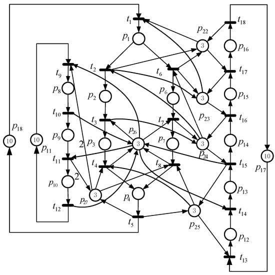
Figure 7. A Petri net model.

Table 9. Iteration steps of the net depicted in Figure 7.

b	RMs	ILMs	LMs	Time
1	15		15	<0.1 s
2	102		102	<0.1 s
3	518		518	<0.1 s
4	1975		1975	1.2 s
5	5912		5912	6.3 s
6	14,306	9	14,297	36.7 s
7	28,190	60	28,130	201.5 s
8	45,382	233	45,149	940.3 s
9	59,410	653	58,757	2041.7 s
10	62,068	1246	60,822	2240.2 s
11	50,452	1766	48,686	2629.9 s
12	30,791	1832	28,959	2385.6 s
13	13,199	1167	12,032	2238.3 s
14	3509	416	3093	1670.2 s
15	399	56	343	1373.3 s
total	316,228	7438	308,790	<15,765.5 s

Table 10. Performance comparison of different methods.

Parameters	[24]	[26]	Proposed Method
No. RMs	2,067,661	2,067,661	316,228
No. LMs	2,032,573	2,032,573	308,790
Time	<16,620.4 s	<154,922.7 s	<15,765.5 s

4. Conclusions

This paper introduces a TGAL-based approach to calculate and analyze the RG of Petri net models. Given a generalized net system, this method systematically generates its RG through the introduction of a GIP. At each iteration, the previously obtained states are selected to compute and classify the RMs of the current step. During an iterative process, a system state is required to be computed and analyzed only once. In terms of time complexity and space complexity, this approach outperforms the techniques in [24,26]. In particular, it has more advantages in terms of computation time than our previous algorithms in [26,27]. Furthermore, compared with the techniques in [13,14], the proposed method has an advantage in terms of space complexity since RMs are partially generated at each iteration step. Consequently, this method is more advantageous than the approaches in [13,14] to compute the RG of a large-scale net system. Nevertheless, the proposed method also exhibits a drawback, i.e., it involves frequently reading and writing a large number of states at each iteration. One of our future research directions is to consider improving the state storage method to enhance the efficiency of the algorithm for complex systems. Another is to extend the proposed method to other types of Petri nets, such as time Petri nets, colored Petri nets, and object Petri nets.

Appendix A.1. Petri Nets

A Petri net [28] is a quadruple $N=(P,T,F,W)$, where P and T are finite and non-empty sets of places and transitions, respectively. The flow relation of a net is represented by arcs with arrows from places to transitions or from transitions to places, denoted as $F\subseteq (P\times T)\cup (T\times P)$. $W:(P\times T)\cup (T\times P)\to \mathbb{N}$ is a mapping that assigns a weight to an arc: $W(x,y)>0$ if $(x,y)\in F$, and $W(x,y)=0$ otherwise, where $x,y\in P\cup T$ and $\mathbb{N}$ comprise the set of non-negative integers. The preset and postset of a node $x\in P\cup T$ are ${}_{ }{}^{•}x_{ }^{ }=\{y\in P\cup T\mid (y,x)\in F\}$ and ${}_{ }{}^{ }x_{ }^{•}=\{y\in P\cup T\mid (x,y)\in F\}$, respectively. Furthermore, the preset and postset of a set $X\subseteq P\cup T$ are ${}_{ }{}^{•}X_{ }^{ }=\{y\in P\cup T\mid y\in {}_{ }{}^{•}x_{ }^{ }\wedge x\in X\}$ and ${}_{ }{}^{ }X_{ }^{•}=\{y\in P\cup T\mid y\in x^{•}\wedge x\in X\}$, respectively. A marking represents a mapping $M:P\to \mathbb{N}$. The number of tokens in place p at marking M is denoted as $M\left(p\right)$. Generally, marking M can be written as ${\sum }_{p\in P}M\left(p\right)p$. The pair $(N,M_0)$ is called a marked Petri net or a net system. Incidence matrix $\left[N\right]$ of net N is a $\left|P\right|\times \left|T\right|$ integer matrix with $\left[N\right](p,t)=W(t,p)-W(p,t)$.

A transition $t\in T$ is enabled at marking M if for all $p\in {}_{ }{}^{•}t_{ }^{ }$, $M\left(p\right)\ge W(p,t)$. This fact is denoted as $M[t⟩$. Once a transition t fires, it yields a marking $M^{\prime }$, denoted as $M[t⟩M^{\prime }$, where $M^{\prime }\left(p\right)=M\left(p\right)-W(p,t)+W(t,p)$, for all $p\in P$. Marking $M^{″}$ is said to be an RM from $M^{\prime }$ if there is a sequence of transitions $\sigma =t_1{t}_2\cdots t_n$ such that $M^{\prime }[\sigma ⟩M^{″}$ holds. $M_0[⟩$ is called the set of RMs of a net model N from the initial marking $M_0$, often denoted by $R(N,M_0)$. An RG is a graphical representation of $R(N,M_0)$, whose nodes are markings in $R(N,M_0)$ and whose arcs are labeled by the transitions of N, denoted as $G(N,M_0)$.

Let $(N,M_0)$ be a net system with $N=(P,T,F,W)$. A transition $t\in T$ is live at $M_0$ if for all $M\in R(N,M_0)$, there is $M^{\prime }\in R(N,M)$ such that $M^{\prime }[t⟩$ holds. $(N,M_0)$ is live if for all $t\in T$, t is live at $M_0$. It is dead at $M_0$ if there is not a transition $t\in T$ such that $M_0[t⟩$ holds.

Appendix A.2. Analysis of Reachability Graph

In [27], a manufacturing-oriented Petri net (M-net for short) is introduced, which is a generalization of the models for flexible manufacturing systems (FMSs). In an M-net, places can be partitioned into three types: idle, operation (activity), and resource places, whose sets are denoted as $P^0$, $P_A$, and $P_R$, respectively. An idle place represents a raw part before entering a production sequence. The token count in an idle place denotes the number of concurrent operations that can happen in the production sequences. An operation place means an operation to be processed for a part in a production sequence, and initially it has no token. A resource place signifies types of available resources, such as robots and machines. In the initial state, tokens in a resource place are equal to the number of available resource units.

Given a deadlock-free control specification for a net model $(N,M_0)$, a marking is legal if its successor can go back to the initial marking; otherwise, it is an ILM. The set of LMs, denoted as ${\mathcal{M}}_{\mathrm{L}}$, is defined as

$${\mathcal{M}}_{\mathrm{L}}=\{M\in R(N,M_0)|M_0\in R(N,M)\}.$$

Meanwhile, the set of ILMs, denoted as ${\mathcal{M}}_{\overline{\mathrm{L}}}$, is defined as

$${\mathcal{M}}_{\overline{\mathrm{L}}}=R(N,M_0)\setminus {\mathcal{M}}_{\mathrm{L}}.$$

References

- Coffman, E.G.; Elphick, M.J.; Shoshani, A. Systems deadlocks. ACM Comput. Surv. 1971, 3, 67–78. [Google Scholar] [CrossRef]
- Yamalidou, K.; Moody, J.; Lemmon, M.; Antsaklis, P. Feedback control of Petri nets based on place invariants. Automatica 1996, 32, 15–28. [Google Scholar] [CrossRef]
- Tricas, F.; Garcia-Valles, F.; Colom, J.M.; Ezpeleta, J. An Iterative Method for Deadlock Prevention in FMS; Springer: New York, NY, USA, 2000. [Google Scholar]
- Dou, H.; You, D.; Wang, S.G.; Zhou, M.C. Designing liveness-enforcing supervisors for manufacturing systems by using maximally good step graphs of Petri nets. IEEE Trans. Autom. Sci. Eng. 2024, 1–12. [Google Scholar] [CrossRef]
- Abubakar, U.S.; Liu, G.Y. Adaptive supervisory control for automated manufacturing systems using borrowed-buffer slots. Inf. Sci. 2024, 667, 1–15. [Google Scholar] [CrossRef]
- Ezpeleta, J.; Tricas, F.; Garcia-Valles, F.; Colom, J.M. A banker’s solution for deadlock avoidance in FMS with flexible routing and multiresource states. IEEE Trans. Robot. Autom. 2002, 18, 621–625. [Google Scholar] [CrossRef]
- Du, N.; Hu, H.S.; Zhou, M.C. Robust deadlock avoidance and control of automated manufacturing systems with assembly operations using Petri nets. IEEE Trans. Autom. Sci. Eng. 2020, 17, 1961–1975. [Google Scholar] [CrossRef]
- Liu, G.Y.; Li, P.; Wu, N.Q.; Yin, L. Two-step approach to robust deadlock control in automated manufacturing systems with multiple resource failures. J. Chin. Inst. Eng. 2018, 41, 484–494. [Google Scholar] [CrossRef]
- Giua, A. Supervisory control of Petri nets with language specifications. In Control of Discrete-Event Systems; Springer: Berlin/Heidelberg, Germany, 2013; pp. 235–255. [Google Scholar]
- Attar, M.; Lucia, W. Data-driven robust backward reachable sets for set-theoretic model predictive control. IEEE Control. Syst. Lett. 2023, 7, 2305–2310. [Google Scholar] [CrossRef]
- Wang, S.G.; Wang, C.Y.; Zhou, M.C. Controllability conditions of resultant siphons in a class of Petri nets. IEEE Trans. Syst. Man Cybern.—Part A Syst. Humans 2012, 42, 1206–1215. [Google Scholar] [CrossRef]
- Hu, H.S.; Liu, Y.; Zhou, M.C. Maximally permissive distributed control of large scale automated manufacturing systems modeled with Petri nets. IEEE Trans. Control. Syst. Technol. 2015, 23, 2026–2034. [Google Scholar]
- Huang, Y.S.; Pan, Y.L.; Zhou, M.C. Computationally improved optimal deadlock control policy for flexible manufacturing systems. IEEE Trans. Syst. Man Cybern.—Part A Syst. Humans 2012, 42, 404–415. [Google Scholar] [CrossRef]
- Huang, Y.S.; Chung, T.H.; Su, P.J. Synthesis of deadlock prevention policy using Petri nets reachability graph technique. Asian J. Control 2010, 12, 336–346. [Google Scholar] [CrossRef]
- Yang, B.Y.; Hu, H.S. Maximally permissive deadlock and livelock avoidance for automated manufacturing systems via critical distance. IEEE Trans. Autom. Sci. Eng. 2022, 19, 3838–3852. [Google Scholar] [CrossRef]
- Ghaffari, A.; Rezg, N.; Xie, X.L. Design of a live and maximally permissive Petri net controller using the theory of regions. IEEE Trans. Robot. Autom. 2003, 19, 137–141. [Google Scholar] [CrossRef]
- Hu, H.S.; Liu, Y. Supervisor simplification for AMS based on Petri nets and inequality analysis. IEEE Trans. Autom. Sci. Eng. 2013, 11, 66–77. [Google Scholar] [CrossRef]
- Pastor, E.; Cortadella, J.; Roig, O. Symbolic analysis of bounded Petri nets. IEEE Trans. Comput. 2001, 50, 432–448. [Google Scholar] [CrossRef]
- Chen, Y.F.; Li, Z.W.; Khalgui, M.; Mosbahi, O. Design of a maximally permissive liveness-enforcing Petri net supervisor for flexible manufacturing systems. IEEE Trans. Autom. Sci. Eng. 2011, 8, 374–393. [Google Scholar] [CrossRef]
- Miner, A.S.; Ciardo, G. Efficient reachability set generation and storage using decision diagrams. In Lecture Notes in Computer Science; Springer: Berlin/Heidelberg, Germany, 1999; Volume 1639, pp. 6–250. [Google Scholar]
- Pastor, E.; Cortadella, J.; Roig, O.; Badia, R.M. Petri net analysis using Boolean manipulation. In Lecture Notes in Computer Science; Springer: Berlin/Heidelberg, Germany, 1994; Volume 815, pp. 416–435. [Google Scholar]
- Ma, Z.Y.; Tong, Y.; Li, Z.W.; Giua, A. Basis marking representation of Petri net reachability spaces and its application to the reachability problem. IEEE Trans. Autom. Control. 2017, 62, 1078–1093. [Google Scholar] [CrossRef]
- Dong, Y.F.; Li, Z.W.; Wu, N.Q. Symbolic verification of current-state opacity of discrete event systems using Petri nets. IEEE Trans. Syst. Man Cybern. Syst. 2022, 52, 7628–7641. [Google Scholar] [CrossRef]
- Uzam, M.; Li, Z.W.; Abubakar, U.S. Think-globally-act-locally approach for the synthesis of a liveness-enforcing supervisor of FMSs based on Petri nets. Int. J. Prod. Res. 2016, 54, 4634–4657. [Google Scholar] [CrossRef]
- Uzam, M.; Gelen, G.; Saleh, T.L. Think-globally-act-locally approach with weighted arcs to the synthesis of a liveness-enforcing supervisor for generalized Petri nets modeling FMSs. Inf. Sci. 2016, 363, 235–260. [Google Scholar] [CrossRef]
- Li, C.Z.; Chen, Y.F.; Li, Z.W.; Barkaoui, K. Synthesis of liveness-enforcing Petri net supervisors based on think-globally-act-locally approach and vector covering for flexible manufacturing systems. IEEE Access 2017, 5, 16349–16358. [Google Scholar] [CrossRef]
- Li, C.Z.; Li, Y.Y.; Chen, Y.F.; Wu, N.Q.; Li, Z.W.; Ma, P.Y.; Kaid, H. Synthesis of liveness-enforcing Petri net supervisors based on a think-globally-act-locally approach and a structurally minimal method for flexible manufacturing systems. Comput. Inform. 2022, 41, 1310–1336. [Google Scholar] [CrossRef]
- Murata, T. Petri nets: Properties, analysis and applications. Proc. IEEE 1989, 77, 541–580. [Google Scholar] [CrossRef]
- Ezpeleta, J.; Colom, J.M.; Martinez, J. A Petri net based deadlock prevention policy for flexible manufacturing systems. IEEE Trans. Robot. Autom. 1995, 11, 173–184. [Google Scholar] [CrossRef]
Disclaimer/Publisher’s Note: The statements, opinions and data contained in all publications are solely those of the individual author(s) and contributor(s) and not of MDPI and/or the editor(s). MDPI and/or the editor(s) disclaim responsibility for any injury to people or property resulting from any ideas, methods, instructions or products referred to in the content. |
© 2025 by the authors. Licensee MDPI, Basel, Switzerland. This article is an open access article distributed under the terms and conditions of the Creative Commons Attribution (CC BY) license (https://creativecommons.org/licenses/by/4.0/).