Bayesian Estimation of the Stress–Strength Parameter for Bivariate Normal Distribution Under an Updated Type-II Hybrid Censoring

Abstract

To save time and cost for a parameter inference, the type-II hybrid censoring scheme has been broadly applied to collect one-component samples. In the current study, one of the essential parameters for comparing two distributions, that is, the stress–strength probability $\delta =Pr(X<Y)$, is investigated under a new proposed type-II hybrid censoring scheme that generates the type-II hybrid censored two-component sample from the bivariate normal distribution. The difficult issues occurred from extending the one-component type-II hybrid censored sample to a two-component type-II hybrid censored sample are keeping useful information from both components and the establishment of the corresponding likelihood function. To conquer these two drawbacks, the proposed type-II hybrid censoring scheme is addressed as follows. The observed values of the first component, X, of data pairs $(X,Y)$ are recorded up to a random time $\tau =max\{X_{r:n},T\}$, where $X_{r:n}$ is the rth ordered statistic among n items with $r<n$ as two pre-specified positive integers and T is a pre-determined experimental time. The observed value from the other component variable Y is recorded only if it is the counterpart of X and also observed before time $\tau$; otherwise, it is denoted as occurred or not at $\tau$. Under the new proposed scheme, the likelihood function of the new bivariate censored data is derived to include the factors of double improper integrals to cover all possible cases without the loss of data information where any component is unobserved. A Monte Carlo Markov chain (MCMC) method is applied to find the Bayesian estimate of the bivariate distribution model parameters and the stress–strength probability, $\delta$. An extensive simulation study is conducted to demonstrate the performance of the developed methods. Finally, the proposed methodologies are applied to a type-II hybrid censored sample generated from a bivariate normal distribution.

1. Introduction

The model of stress–strength has attracted broad consideration by researchers in diverse aspects for numerous years. Among them, the quantity $\delta =Pr(X<Y)$ is of the most interest, with X and Y as two random characteristic measurements from two competitive components in a system. In the application of biometry, let X and Y be the remaining survival times after patients are treated with drug A and drug B, respectively. Then, the probability $\delta \ge 1/2$ can be applied as an assessment to select the treatment utilizing drug A or B. For engineering or industrial study, $\delta$ is utilized to gauge the reliability of an event indicating the random strength of a component Y over the stress of a competitive factor X. When random variables X and Y are probability independent, Birnbaum [1] provided a brilliant relationship between the classical Mann–Whitney statistic and $\delta$. Up to the present, the investigation of estimation methods for $\delta$ under various distributions and life test settings have appeared in statistical literature. Examples include Enis and Geisser [2] under exponential or normal distributions for both stress and strength using Bayesian procedure; Tong [3] under negative exponential distribution using minimum variance and unbiased estimation; Bai and Hong [4] under two-parameter exponential distributions with common location parameter using uniformly minimum variance unbiased and maximum likelihood estimations; Surles and Padgett [5,6] under Burr X distributions using maximum likelihood and Bayesian estimations; Ali et al. [7] under two-parameter exponential distribution using maximum likelihood procedure for many different cases; Kim and Chung [8] under Burr X distribution using Bayesian estimation; Kundu and Gupta [9,10] under generalized exponential and Weibull distribution using maximum likelihood, minimum variance unbiased, and Bayesian estimations; Saracoglu and Kaya [11] under Gompertz distribution using maximum likelihood estimation; Raqab et al. [12] under three-parameter generalized exponential distribution using a modified maximum likelihood and Bayesian estimations; Kundu and Raqab [13] under three-parameter Weibull distribution using modified maximum likelihood and approximate maximum likelihood estimations; Saracoglu et al. [14] under Gompertz distribution using maximum likelihood, uniformly minimum variance unbiased, and Bayesian estimations; and Genç [15] under the standard Topp–Leone distribution using maximum likelihood and uniformly minimum variance unbiased estimation procedures. The aforementioned references were for complete random samples. Kotz et al. [16] presented a wonderful collection of the developments on estimations of $\delta$.

Because of technology advancement, the products’ lifetimes have been prolonged. Often, collecting a complete random lifetime sample from the life test experiment could be difficult. Thus, more research investigation has implemented numerous diverse approaches to adjust this downside. Type-I and II censoring schemes are the most easily used. Let n items be under a life test. The life test under a type-I censoring scheme is terminated at a specific time, T, scheduled ahead, and the remaining survival items are removed and only known to have lifetimes larger than T. For example, Lin and Lio [17] applied the Bayesian estimation for population parameters under progressive type-I interval censoring. Type-II censoring one is terminated at the first r failures observed where r was decided in advance. A generalized type-II censoring was a progressive type-II one, where $R_i$ survived items are randomly removed from experiment at the ith observed failure time for i from $1,2,3,\dots ,r$ and $R_i,i=1,2,3,\dots ,r$ were decided in advance such that ${\sum }_{j=1}^r{R}_j=n-m$. The probability inference of reliability analysis utilizing the progressively type-II censored samples has been done for many years. For example, Saracoglu et al. [18] studied the estimation problem of $\delta$ based on progressively type-II censored samples from two independent exponential distributions, and Çiftci et al. [19] worked on estimation of $\delta$ for a generalized Gompertz distribution under progressive type-II censoring. One may refer to the review papers by Balakrishnan [20] and the two books on progressive censoring by Balakrishnan and Aggarwala [21] and Balakrishnan and Cramer [22] for more information regarding the theory and applications of progressive censoring.

Under univariate distribution, Epstein [23] proposed a type-I hybrid censoring scheme where the test was terminated at the random time ${\tau }_{*}=min\{X_{r:n},T\}$, where $X_{r:n}$ is the rth ordered statistic among n items with $r<n$ as two pre-specified positive integers and T is a pre-determined experimental time. It was a flexible mixture of type-I and type-II censoring schemes since it generalized the idea of type-II censoring that only at most the first r observations of main variable X were observed and a predetermined time T was placed to terminate the experiment. Some similar studies, such as Childs et al. [24] and Hyun et al. [25], considered a type-II hybrid censoring scheme with stopping time at the random time $\tau =max\{X_{r:n},T\}$ that ensures r failures observed among n items. Under bivariate distribution, Balakrishnan and Kim [26] analyzed the type-II bivariate normal data with maximum likelihood estimation method. Lin et al. [27] and Lin et al. [28] studied the Bayesian estimation methods for the model parameters and stress–strength reliability, respectively, with type-II censoring from a Downton bivariate exponential distribution with positive correlation. These bivariate studies of type-II scheme mainly focused on the first r statistics of variable X; the experiment was not terminated until all the concomitant Y variates were observed and the survival information of other Y variates was also ignored. To remedy the above problem, a new type-II hybrid censoring scheme is proposed to study the strength reliability model $\delta$, where X and Y have the joint bivariate normal distribution. Under the proposed updated type-II hybrid censoring scheme, X and the concomitant Y is recorded as follows. If an observed value of $X\le \tau$ then the value of X is recorded; otherwise, it is replaced by not occurred. At the same time, the value of Y is recorded if it is the concomitant of observed X and also occurs before or at $\tau$. For the remaining observations of Y, they are recorded as occurred or not occurred according to whether $Y\le \tau$ or not. The current research work is focused on the point estimation of the stress–strength $\delta$ through the Bayesian approach based on the proposed type-II hybrid censored samples from bivariate normal distribution.

The remainder of the paper is organized as follows. The likelihood function based on the proposed type-II hybrid censored sample from the bivariate normal distribution is presented in Section 2. Two MCMC methods are applied to estimate the model parameters, and the reliability parameter $\delta$ is discussed in Section 3. A Monte Carlo simulation study to evaluate the performance of the estimation method is provided in Section 4. Section 5 illustrates the proposed methodology by utilizing a numerical example. Finally, some discussions and concluding remarks are given in Section 6.

2. Model and Notations

Let two-component random vector $(X,Y)$ follow the five-parameter bivariate normal distribution (BVN) with parameters $-\infty <{\mu }_1<\infty ,-\infty <{\mu }_2<\infty ,0<{\sigma }_1^2,{\sigma }_2^2$ and $-1\le \rho \le 1$, denoted as BVN$({\mu }_1,{\mu }_2,{\sigma }_1^2,{\sigma }_2^2,\rho )$, the joint probability density function (PDF) is given by

$$\begin{array}{c}\hfill f(x,y)={\displaystyle \frac{1/\sqrt{1-{\rho }^2}}{2\pi {\sigma }_1{\sigma }_2}}exp\left\{{\displaystyle \frac{-1}{2(1-{\rho }^2)}}\left[{\left({\displaystyle \frac{x-{\mu }_1}{{\sigma }_1}}\right)}^2-2\rho {\displaystyle \frac{(x-{\mu }_1)(y-{\mu }_2)}{{\sigma }_1{\sigma }_2}}+{\left({\displaystyle \frac{y-{\mu }_2}{{\sigma }_2}}\right)}^2\right]\right\},\end{array}$$

(1)

where ${\mu }_1$ and ${\mu }_2$ are the marginal means of X and Y, $0<{\sigma }_1$ and $0<{\sigma }_2$ are the marginal standard deviations of X and Y, and $\rho$ is the correlation coefficient of X and Y.

Moreover, it can be seen that $Y-X\sim N({\mu }_2-{\mu }_1,{\sigma }_1^2+{\sigma }_2^2-2\rho {\sigma }_1{\sigma }_2)$, which is the normal distribution with mean ${\mu }_2-{\mu }_1$ and variance ${\sigma }_1^2+{\sigma }_2^2-2\rho {\sigma }_1{\sigma }_2$. Therefore, the reliability probability can be easily derived as

$$\begin{array}{c}\hfill \delta =\mathrm{\Phi }\left({\displaystyle \frac{{\mu }_2-{\mu }_1}{\begin{array}{c}\hfill \sqrt{{\sigma }_1^2+{\sigma }_2^2-2\rho {\sigma }_1{\sigma }_2}\end{array}}}\right),\end{array}$$

(2)

where $\mathrm{\Phi }\left(z\right)$ is the standard normal distribution function. The estimation of parameter $\rho$ has been studied by many authors. For example, Al-Saadi and Young [29] derived the method of moment estimator for $\rho$ through equating a population mixed moments and sample mixed moments and suggested a modified method of moments estimator through a standard bias reduction method. They also suggested a bias-reduced estimator based on the sample correlation coefficient. Balakrishnan and Ng [30] modified the estimation procedures of Al-Saadi and Young [29] and derived an improved method of moments estimator using the standard bias reduction and Jackknife methods. These aforementioned estimation procedures for $\rho$ were based on complete random samples.

The conditional distribution of Y given $X=x$ follows $N({\mu }_2+\rho {\displaystyle \frac{{\sigma }_2}{{\sigma }_1}}(x-{\mu }_1),(1-{\rho }^2){\sigma }_2^2)$. Therefore, the joint pdf of the BVN$(\overrightarrow{m},\Sigma )$ can be expressed as

$$\begin{array}{cc}\hfill f\left(\overrightarrow{x}\right)& =f_X\left(x\right)f_{Y|X}\left(y\right|x)\hfill \\ \hfill & ={\displaystyle \frac{1}{\sqrt{2\pi }{\sigma }_1}}exp\left(-{\displaystyle \frac{{(x-{\mu }_1)}^2}{2{\sigma }_1^2}}\right){\displaystyle \frac{1}{\sqrt{2\pi }{\sigma }_2\sqrt{1-{\rho }^2}}}exp\left({\displaystyle \frac{-{\left(y-{\mu }_2-\rho \frac{{\sigma }_2}{{\sigma }_1}(x-{\mu }_1)\right)}^2}{2(1-{\rho }^2){\sigma }_2^2}}\right),\hfill \end{array}$$

(3)

where $f_X\left(x\right)$ is the pdf of the normal distribution with mean ${\mu }_1$ and variance ${\sigma }_1^2$, and $f_{Y|X}\left(y\right|x)$ is the corresponding conditional pdf of Y, given $X=x$. For more information about bivariate normal distribution, readers can refer to Balakrishnan and Kim [26].

2.1. Type-II Censoring Scheme

From a given random sample of size n, $(x_i,y_i),i=1,2,\cdots ,n$, from BVN$(\overrightarrow{m},\Sigma )$, let $x_{1:n}\le x_{2:n}\le \cdots \le x_{n:n}$ be the order statistics of the x-sample and $y_{[i:n]}$ be the corresponding value of Y associated with $x_{i:n}$ for $i=1,2,\cdots ,n$. Then $D_r={\left\{(x_{j:n},y_{[j:n]})\right\}}_{j=1}^r$ is defined as the observed type-II censored sample, and the corresponding likelihood of $D_r$ without constant factor is

$$\begin{array}{cc}\hfill L_r({\mu }_1,{\mu }_2,\rho )& =\prod _{i=1}^{r}f(x_{i:n},y_{[i:n]})\prod _{i=r+1}^{N}Pr(X>x_{r:n})\hfill \\ \hfill & ={\left({\displaystyle \frac{1}{2\pi {\sigma }_1{\sigma }_2\sqrt{1-{\rho }^2}}}\right)}^{r}exp\left\{{\displaystyle \frac{-1}{2(1-{\rho }^2)}}\sum _{i=1}^r{\theta }_i(x_{i:n},y_{[i:n]},{\mu }_1,{\mu }_2,{\sigma }_1,{\sigma }_2,\rho )\right\}\hfill \\ \hfill & {\left(1-\mathrm{\Phi }\left({\displaystyle \frac{x_{r:n}-{\mu }_1}{{\sigma }_1}}\right)\right)}^{N-r},\hfill \end{array}$$

(4)

where

$$\begin{array}{c}\hfill {\theta }_i(x_{i:n},y_{[i:n]},{\mu }_1,{\mu }_2,{\sigma }_1,{\sigma }_2,\rho )={\left({\displaystyle \frac{x_{i:n}-{\mu }_1}{{\sigma }_1}}\right)}^2-2\rho {\displaystyle \frac{(x_{i:n}-{\mu }_1)(y_{[i:n]}-{\mu }_2)}{{\sigma }_1{\sigma }_2}}+{\left({\displaystyle \frac{y_{[i:n]}-{\mu }_2}{{\sigma }_2}}\right)}^2.\end{array}$$

However, it could need more time over T and $x_{r:n}$ to collect all $y_{[j:n]}$ for $j=1,2,\cdots ,r$. Therefore, a new censoring scheme named type-II hybrid one for bivariate model is proposed next.

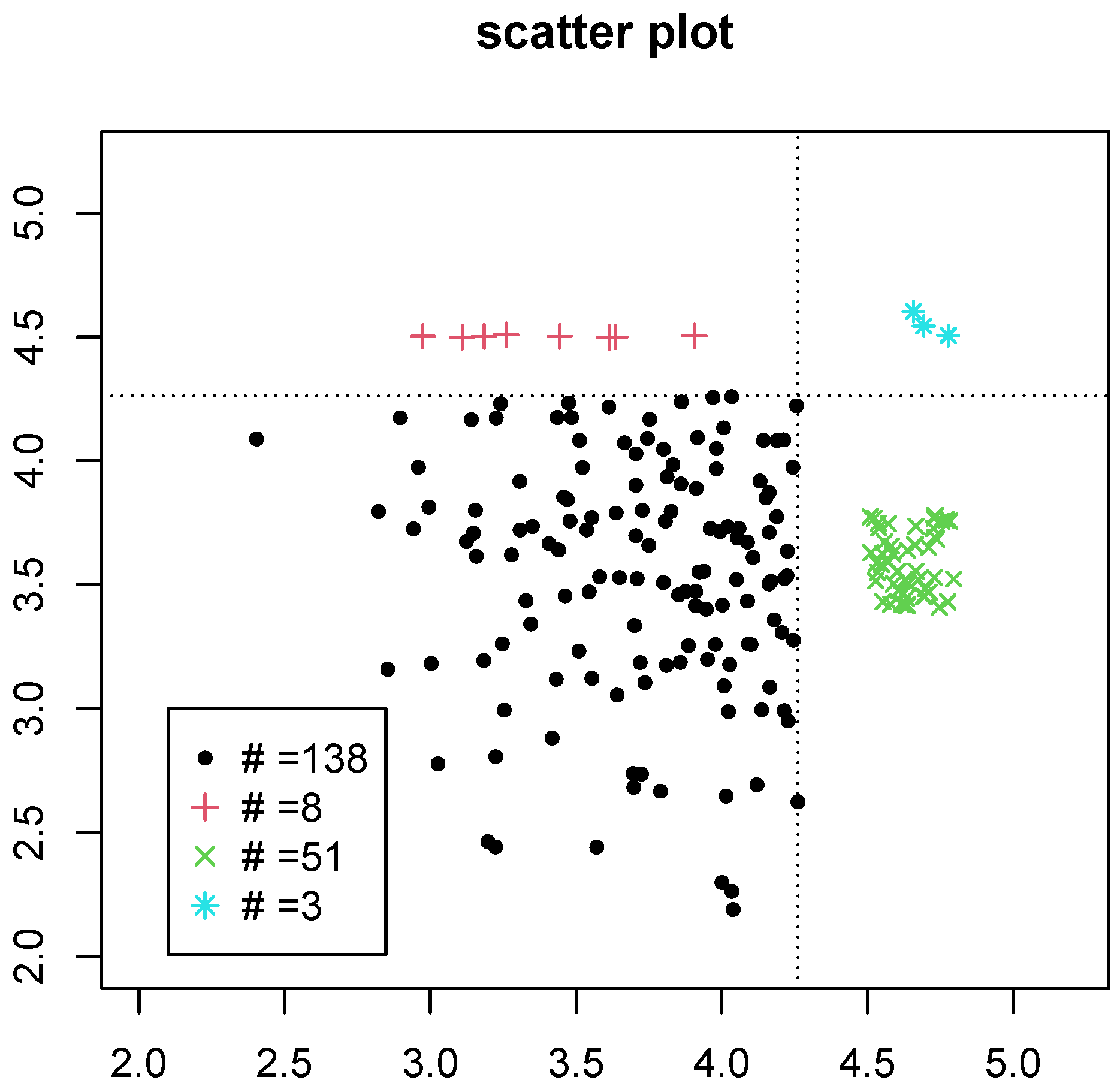
2.2. Updated Type-II Hybrid Censoring Scheme

A new censoring scheme is named updated type-II hybrid censoring scheme for collecting samples from a bivariate distribution. The updated type-II hybrid censoring scheme, which had been mentioned in the abstract and Section 1, generalizes the type-II hybrid data of the first component X of $\overrightarrow{X}$ up to the random time $\tau$ and combines the survival information of the concomitant Y. The failure time of variable X is recorded up to the experiment stopping time $\tau$; otherwise, it is truncated. The value of Y is also recorded only if Y is the concomitant of observed X and its value is observed before or at $\tau$. Moreover, if Y is not a concomitant of an observed X, then it is denoted as occurred or not at $\tau$ depending on the event $\{Y\le \tau \}$ or $\{Y>\tau \}$.

Specifically, letting $\overrightarrow{x}$ be a pair of realizations from BVN$(\overrightarrow{m},\Sigma )$, each pair $(x^{*},y^{*})$ of the updated type-II hybrid censored data $D^{*}={\left\{(x_i^{*},y_i^{*})\right\}}_{i=1}^n$ belongs to exactly one of the following four data types:

1

If $x\le \tau$, $y\le \tau$; both x and y are observed. Denote $(x^{*},y^{*})=(x,y)$.

2

If $x\le \tau$, $y>\tau$; only x is observed and y is truncated at $\tau$ and recorded as +. Denote $(x^{*},y^{*})=(x,+)$.

3

If $x>\tau$, $y<\tau$; x is truncated at $\tau$, and y is only recorded as −. Denote $(x^{*},y^{*})=(+,-)$.

4

If $x>\tau$; $y>\tau$; both x and y are not observed and they are truncated at $\tau$. Denote $(x^{*},y^{*})=(+,+)$.

Let $n_1$, $n_2$, $n_3$, and $n_4$ be the numbers of the sets of data type 1, 2, 3, and 4, respectively, and $n=n_1+n_2+n_3+n_4$. The censored data $D^{*}={\left\{(x_i^{*},y_i^{*})\right\}}_{i=1}^n$ is equivalently written as

$$D^{*}={\left\{(x_i,y_i)\right\}}_{i=1}^{n_1}\mathrm{or}{\left\{(x_i,+)\right\}}_{i=1}^{n_2}\mathrm{or}{\left\{(+,-)\right\}}_{i=1}^{n_3}\mathrm{or}{\left\{(+,+)\right\}}_{i=1}^{n_4},$$

where $\left\{(x_i,y_i)\right\},i=1,2,\cdots ,n$, is a complete dataset from the BVN distribution.

2.3. The Likelihood of Updated Type-II Hybrid Data

The likelihood of pair ($x^{*},y^{*})$ under the updated type-II hybrid censoring can be calculated case by case as follows. The derivations of the likelihood functions are shown in Appendix A.

• The likelihood of $(x^{*},y^{*})=(x,y)$ is the same as the pdf in Equation (1). That is,

  $$\begin{array}{c}\hfill f_1(x^{*},y^{*})={\displaystyle \frac{1}{2\pi {\sigma }_1{\sigma }_2\sqrt{1-{\rho }^2}}}{exp}^{{\displaystyle \frac{-1}{2(1-{\rho }^2)}}\left[{\left({\displaystyle \frac{x-{\mu }_1}{{\sigma }_1}}\right)}^2-2\rho {\displaystyle \frac{(x-{\mu }_1)(y-{\mu }_2)}{{\sigma }_1{\sigma }_2}}+{\left({\displaystyle \frac{y-{\mu }_2}{{\sigma }_2}}\right)}^2\right]}.\end{array}$$

  (5)
• The likelihood of $(x^{*},y^{*})=(x,+)$ can be integrated.

  $$\begin{array}{ccc}\hfill f_2(x^{*},y^{*})& ={\displaystyle \frac{1}{\sqrt{2\pi }{\sigma }_1}}exp\left\{{\displaystyle \frac{-{(x-{\mu }_1)}^2}{2{\sigma }_1^2}}\right\}\left(1-\mathrm{\Phi }\left({\displaystyle \frac{\tau -{\mu }_2-\rho \frac{{\sigma }_2}{{\sigma }_1}(x-{\mu }_1)}{{\sigma }_2\sqrt{1-{\rho }^2}}}\right)\right)\hfill & \hfill \end{array}$$

  (6)

  where $\mathrm{\Phi }\left(z\right)$ is the standard normal cdf.
• The likelihood of $(x^{*},y^{*})=(+,-)$ can be integrated in several ways.

  $$\begin{array}{cc}\hfill f_3(x^{*},y^{*})={\int }_{\tau }^{\infty }{f}_Z\left({\displaystyle \frac{x-{\mu }_1}{{\sigma }_1}}\right)\mathrm{\Phi }\left({\displaystyle \frac{\tau -{\mu }_2-\rho \frac{{\sigma }_2}{{\sigma }_1}(x-{\mu }_1)}{{\sigma }_2\sqrt{1-{\rho }^2}}}\right)dx& \hfill \end{array}$$

  (7)

  where $f_Z\left(z\right)$ is the standard normal pdf. The numerical integration can be carried out by most computing software. For example, the R built-in function ‘integrate’ provides the one dimensional numerical integral. Alternatively,

  $$\begin{array}{ccc}\hfill f_3(x^{*},y^{*})& =F_Y\left(\tau \right)-F_{X,Y}(\tau ,\tau )\hfill & \hfill \end{array}$$

  (8)
  The first term $F_Y\left(y\right)$ is the normal cdf with mean ${\mu }_2$ and variance ${\sigma }_2^2$, and the second term $F_{X,Y}(x,y)$ is the bivariate normal cdf, which can be given by some statistical libraries, such as the ‘pmvnorm’ function in the R ‘mvtnorm’ package.
• The likelihood of $(x^{*},y^{*})=(+,+)$ can be integrated in several ways.

  $$\begin{array}{ccc}\hfill f_4(x^{*},y^{*})& ={\int }_{\tau }^{\infty }{f}_Z\left({\displaystyle \frac{x-{\mu }_1}{{\sigma }_1}}\right)\left(1-\mathrm{\Phi }\left({\displaystyle \frac{\tau -{\mu }_2-\rho \frac{{\sigma }_2}{{\sigma }_1}(x-{\mu }_1)}{{\sigma }_2\sqrt{1-{\rho }^2}}}\right)\right)dx.\hfill & \hfill \end{array}$$

  (9)
  Alternatively, the density can be calculated by a bivariate normal cdf.

  $$\begin{array}{cc}\hfill f_4(x^{*},y^{*})& =1-F_X\left(\tau \right)-F_Y\left(\tau \right)+F_{X,Y}(\tau ,\tau ).\hfill \end{array}$$

  (10)

The likelihood function of the proposed censored data $D^{*}=\{(x_i^{*},y_i^{*}),i=1,2,\cdots ,n\}$ can be written as the product of the likelihoods of all pairs $(x_i^{*},y_i^{*})$.

$$\begin{array}{cc}\hfill L({\mu }_1,{\mu }_2,{\sigma }_1^2,{\sigma }_2^2,\rho |D^{*})& =\prod _{i=1}^{n_1}{f}_1(x_i^{*},y_i^{*})\prod _{i=1}^{n_2}{f}_2(x_i^{*},y_i^{*})\prod _{i=1}^{n_3}{f}_3(x_i^{*},y_i^{*})\prod _{i=1}^{n_4}{f}_4(x_i^{*},y_i^{*})\hfill \\ \hfill & ={({\displaystyle \frac{1}{2\pi {\sigma }_1{\sigma }_2\sqrt{1-{\rho }^2}}})}^{n_1}{exp}^{{\displaystyle \frac{-1/2}{1-{\rho }^2}}{\sum }_{i=1}^{n_1}\left[{({\displaystyle \frac{x_i-{\mu }_1}{{\sigma }_1}})}^2-2\rho {\displaystyle \frac{(x_i-{\mu }_1)(y_i-{\mu }_2)}{{\sigma }_1{\sigma }_2}}+{({\displaystyle \frac{y_i-{\mu }_2}{{\sigma }_2}})}^2\right]}\hfill \\ \hfill & {({\displaystyle \frac{1}{\sqrt{2\pi }{\sigma }_1}})}^{n_2}{exp}^{-{\displaystyle \frac{{\sum }_{i=1}^{n_2}{(x-{\mu }_1)}^2}{2{\sigma }_1^2}}}{\left(1-\mathrm{\Phi }({\displaystyle \frac{\tau -{\mu }_2-\rho \frac{{\sigma }_2}{{\sigma }_1}(x-{\mu }_1)}{{\sigma }_2\sqrt{1-{\rho }^2}}})\right)}^{n_2}\hfill \\ \hfill & f_3{(\tau ,\tau )}^{n_3}{f}_4{(\tau ,\tau )}^{n_4}.\hfill \end{array}$$

(11)

The proposed two-component type-II hybrid censored sample is reduced to the type-II hybrid censored sample when the second component, Y, is removed. Note that given i from $\{1,2,3,\cdots ,n\}$, $f_j(x_i^{*},y_i^{*})$ for $j=1,2,3,4$ are defined in Equations (5)–(7) and (9). The maximum likelihood estimation is so far infeasible since the likelihood function in Equation (11), a product of terms involving improper integrals Equations (6), (7) and (9), is too complicated for differentiation methods. The Bayes estimation via the MCMC method can reduce to the obtained estimators similar to the maximum likelihood estimates if non-informative priors are used. See, for example, Chib and Greenberg [31].

3. Bayesian Framework

Under the Bayesian framework, Zhang and Yang [32] demonstrated that the posteriors from independent priors are very close to the posteriors from dependent priors because independent priors are the mean-field variational approximation of dependent priors. Hence, independent priors are used in this study. Let conjugate prior distributions for the unknown parameters, ${\mu }_1$, ${\mu }_2$, be normal distributions, priors for ${\sigma }_1^2$ and ${\sigma }_2^2$ be inverse Gamma, and the prior of $\rho$ follow uniformly over interval $[-1,1]$.

$$\begin{array}{cc}\hfill \pi \left({\mu }_1\right)& \sim \mathbf{N}({\mu }_{10},{\sigma }_{10}^2)\hfill \end{array}$$

(12)

$$\begin{array}{cc}\hfill \pi \left({\mu }_2\right)& \sim \mathbf{N}({\mu }_{20},{\sigma }_{20}^2)\hfill \end{array}$$

(13)

$$\begin{array}{cc}\hfill \pi \left({\sigma }_1^2\right)& \sim \mathbf{Inverse}\mathbf{Gamma}({\alpha }_1,{\beta }_1)\hfill \end{array}$$

(14)

$$\begin{array}{cc}\hfill \pi \left({\sigma }_2^2\right)& \sim \mathbf{Inverse}\mathbf{Gamma}({\alpha }_2,{\beta }_2)\hfill \end{array}$$

(15)

$$\begin{array}{cc}\hfill \pi \left(\rho \right)& \sim \mathbf{Uniform}(-1,1).\hfill \end{array}$$

(16)

Combining Equations (11)–(16), the joint posterior pdf of ${\mu }_1$, ${\mu }_2$, ${\sigma }_1$, ${\sigma }_2$, and $\rho$, based on a type-II hybrid censored sample $D^{*}$, can be expressed as

$$\begin{array}{cc}\hfill \Pi ({\mu }_1,{\mu }_2,{\sigma }_1,{\sigma }_2,\rho |D^{*})& \propto L({\mu }_1,{\mu }_2,{\sigma }_1,{\sigma }_2,\rho |D^{*})\hfill \\ \hfill & \times \pi \left({\mu }_1\right)\pi \left({\mu }_2\right)\pi \left({\sigma }_1^2\right)\hfill \\ \hfill & \times \pi \left({\sigma }_2^2\right)\pi \left(\rho \right).\hfill \end{array}$$

(17)

All these posterior pdfs for the parameters ${\mu }_1$, ${\mu }_2$, ${\sigma }_1$, ${\sigma }_2$, and $\rho$ are not in closed forms, and numerical integration may not be applied to approximate their values either. To obtain the Bayesian estimates, the Markov chain Monte Carlo (MCMC) method through the application of the Metropolis–Hastings (M-H) algorithm (Metropolis et al. [33] and Hastings [34]) via the Gibbs scheme (Geman and Geman [35]) can be utilized to draw the samples of ${\mu }_1$, ${\mu }_2$, ${\sigma }_1$, ${\sigma }_2$, and $\rho$, respectively.

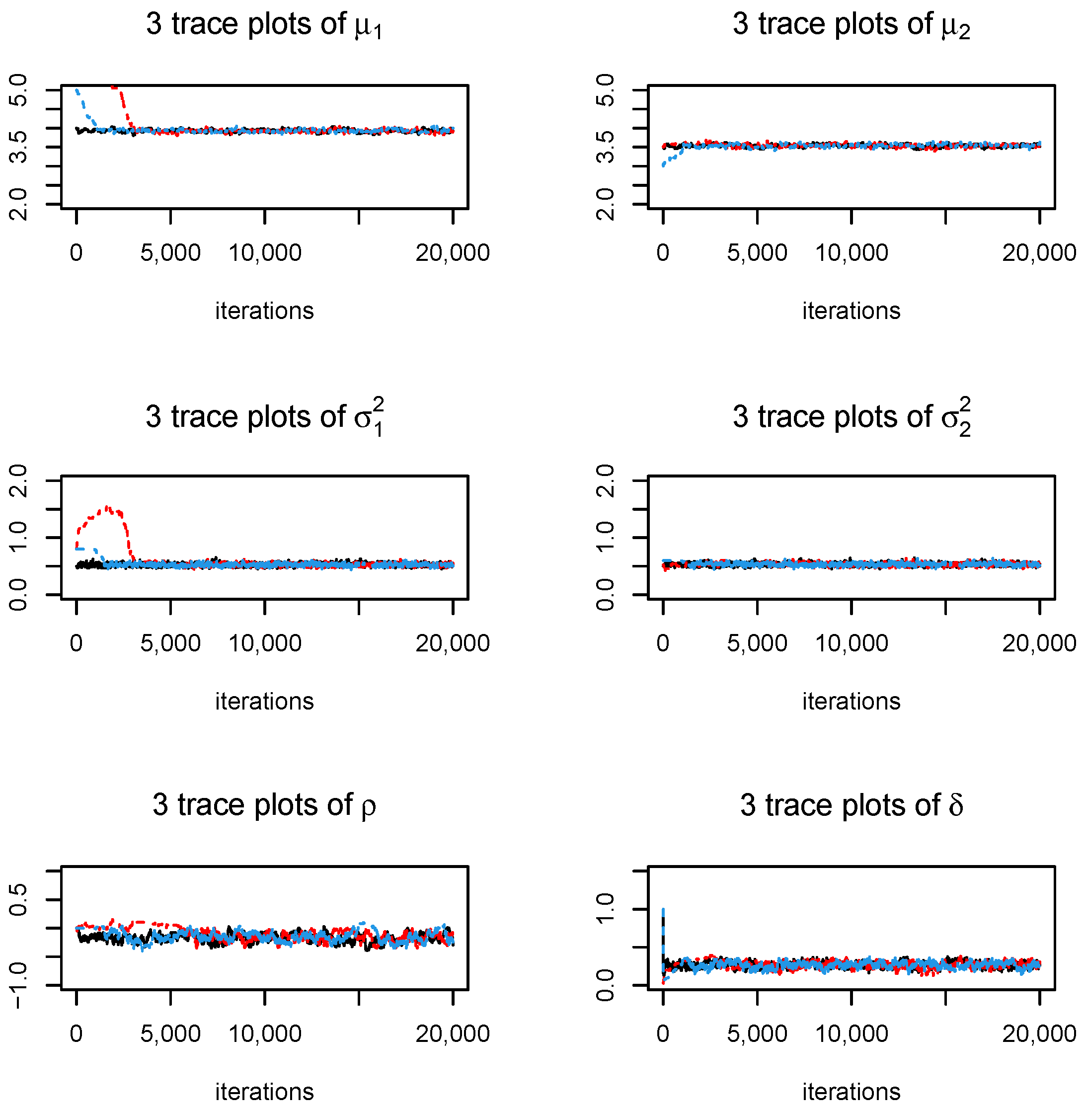
3.1. A Markov Chain Monte Carlo Process

There are several Gibbs sampling strategies in applying the MCMC method. One can update all parameters at once, block by block, or one by one at each Markov chain iteration. Since ${\mu }_1$ and ${\mu }_2$ are the location parameters of the BVN model and ${\sigma }_1,{\sigma }_2,\rho$ are the scale parameters, we consider splitting the parameters into three groups and applying the parameter sampling on these three blocks alternatively. That is, let ${\mathrm{\Theta }}_1=({\mu }_1,{\mu }_2)$ and ${\mathrm{\Theta }}_2=({\sigma }_1,{\sigma }_2,\rho )$. The Gibbs sampling consists of three sachems:

1

sample ${\mathrm{\Theta }}_1|D^{*},{\mathrm{\Theta }}_2$

2

sample ${\mathrm{\Theta }}_2|D^{*},{\mathrm{\Theta }}_1$

3

sample $\delta |D^{*},{\mathrm{\Theta }}_1,{\mathrm{\Theta }}_2$

Then, the Markov chains {${\mathrm{\Theta }}_1^{\left(b\right)},b=1,2,\dots$}, {${\mathrm{\Theta }}_2^{\left(b\right)},b=1,2,\dots$} and {${\delta }^{\left(b\right)},b=1,2,\dots$} of a given parameter, ${\mathrm{\Theta }}_1$, ${\mathrm{\Theta }}_2$, and $\delta$, respectively, can be constructed by applying the M-H algorithm stated as follows.

Let $q\left({\mathrm{\Theta }}_1^{(\ast )}\right|{\mathrm{\Theta }}_1^{(b-1)})$ be a proposed conditional transition probability density function for ${\mathrm{\Theta }}_1^{(\ast )}=({\mu }_1^{(\ast )},{\mu }_2^{(\ast )})$, given ${\mathrm{\Theta }}_1^{(b-1)}=({\mu }_1^{(b-1)},{\mu }_2^{(b-1)})$. Given the current state value, ${\mathrm{\Theta }}_1^{(b-1)}$, of the parameter ${\mathrm{\Theta }}_1$, ${\mathrm{\Theta }}_1^{(\ast )}$ is a candidate value of the parameter ${\mathrm{\Theta }}_1$ in the next state, which can be generated by $q\left({\mathrm{\Theta }}_1^{(\ast )}\right|{\mathrm{\Theta }}_1^{(b-1)})$. Let

$$\begin{array}{cc}\hfill {\pi }_1\left({\mathrm{\Theta }}_1\right|D^{*},{\mathrm{\Theta }}_2)& ={\pi }_1({\mu }_1,{\mu }_2|D^{*},{\sigma }_1,{\sigma }_2,\rho )\hfill \\ \hfill & \propto \prod _{i=1}^{n_1}{f}_1(x_i^{*},y_i^{*})\prod _{i=1}^{n_2}{f}_2(x_i^{*},y_i^{*})\prod _{i=1}^{n_3}{f}_3(x_i^{*},y_i^{*})\prod _{i=1}^{n_4}{f}_4(x_i^{*},y_i^{*})\pi \left({\mu }_1\right)\pi \left({\mu }_2\right)\hfill \end{array}$$

(18)

Then, ${\mathrm{\Theta }}_1^{(\ast )}$ is accepted as the value of the next state, ${\mathrm{\Theta }}_1^{\left(b\right)}$, with the probability of

$${\displaystyle min\left\{1,\frac{{\pi }_1\left({\mathrm{\Theta }}_1^{(\ast )}\right|D^{*},{\mathrm{\Theta }}_2)q\left({\mathrm{\Theta }}_1^{\left(b\right)}\right|{\mathrm{\Theta }}_1^{(\ast )},{\mathrm{\Theta }}_2)}{{\pi }_1\left({\mathrm{\Theta }}_1^{\left(b\right)}\right|D^{*},{\mathrm{\Theta }}_2)q\left({\mathrm{\Theta }}_1^{(\ast )}\right|{\mathrm{\Theta }}_1^{\left(b\right)},{\mathrm{\Theta }}_2)}\right\}.}$$

If ${\mathrm{\Theta }}_1^{(\ast )}$ is rejected as the value of the next state, then the next state ${\mathrm{\Theta }}_1^{\left(b\right)}={\mathrm{\Theta }}_1^{(b-1)}$. Step 2 is similar. Let

$$\begin{array}{cc}\hfill {\pi }_2\left({\mathrm{\Theta }}_2\right|D^{*},{\mathrm{\Theta }}_1)& ={\pi }_2({\sigma }_1,{\sigma }_2,\rho |D^{*},{\mu }_1,{\mu }_2)\hfill \\ \hfill \propto & \prod _{i=1}^{n_1}{f}_1(x_i^{*},y_i^{*})\prod _{i=1}^{n_2}{f}_2(x_i^{*},y_i^{*})\prod _{i=1}^{n_3}{f}_3(x_i^{*},y_i^{*})\prod _{i=1}^{n_4}{f}_4(x_i^{*},y_i^{*})\pi \left({\sigma }_1^2\right)\pi \left({\sigma }_2^2\right)\pi \left(\rho \right)\hfill \end{array}$$

(19)

Then, ${\mathrm{\Theta }}_2^{(\ast )}$ is accepted as the value of the next state, ${\mathrm{\Theta }}_1^{\left(b\right)}$, with the probability of

$${\displaystyle min\left\{1,\frac{{\pi }_2\left({\mathrm{\Theta }}_2^{(*)}\right|D^{*},{\mathrm{\Theta }}_1)q\left({\mathrm{\Theta }}_2^{\left(b\right)}\right|{\mathrm{\Theta }}_1^{(*)})}{{\pi }_2\left({\mathrm{\Theta }}_2^{\left(b\right)}\right|D^{*},{\mathrm{\Theta }}_1)q\left({\mathrm{\Theta }}_2^{(*)}\right|{\mathrm{\Theta }}_2^{\left(b\right)})}\right\}.}$$

If ${\mathrm{\Theta }}_2^{(\ast )}$ is rejected as the value of the next state, then the next state ${\mathrm{\Theta }}_2^{\left(b\right)}={\mathrm{\Theta }}_2^{(b-1)}$.

One of the difficulties in this study is that the distribution of the reliability parameter $\delta$ is not available. Viewing $\delta$ as a latent variable, the data augmentation technique can be applied to implement the state values of $\delta$ and construct a Markov chain. Specifically, given the model parameters’ values ${\mu }_1^{\left(b\right)}$, ${\mu }_2^{\left(b\right)}$, ${\sigma }_1^{\left(b\right)}$, ${\sigma }_2^{\left(b\right)}$, and ${\rho }^{\left(b\right)}$, the state value of ${\delta }^{\left(b\right)}$ can be implemented by the formula in Equation (2). That is,

$${\delta }^{\left(b\right)}=\mathrm{\Phi }\left({\displaystyle \frac{{\mu }_2^{\left(b\right)}-{\mu }_1^{\left(b\right)}}{{\left({\sigma }_1^{\left(b\right)}\right)}^2+{\left({\sigma }_2^{\left(b\right)}\right)}^2-2{\rho }^{\left(b\right)}{\sigma }_1^{\left(b\right)}{\sigma }_2^{\left(b\right)})}}\right)$$

where $\mathrm{\Phi }\left(z\right)$ is the standard normal cdf.

3.2. Bayes Estimation

Starting with initial values, ${\mu }_1^{\left(0\right)}$, ${\mu }_2^{\left(0\right)}$, ${{\sigma }_1^2}^{\left(0\right)}$, ${{\sigma }_2^2}^{\left(0\right)}$, ${\rho }^{\left(0\right)}$, and ${\delta }^{\left(0\right)}$, the above iterative process is run through a huge number of periods (say, N). The empirical distributions of ${\mu }_1$, ${\mu }_2$, ${\sigma }_1^2$, ${\sigma }_2^2$, and $\rho$ could be described by the realizations of ${\mu }_1$, ${\mu }_2$, ${\sigma }_1^2$, ${\sigma }_2^2$, and $\rho$ after a burn-in period, $N_b$. The Bayes estimators of ${\mu }_1$, ${\mu }_2$, and $\rho$ can be approximated based on the values of ${\left\{{\mu }_1^{\left(b\right)}\right\}}_{b=N_b}^N$, ${\left\{{\mu }_2^{\left(b\right)}\right\}}_{b=N_b}^N$, ${\left\{{{\sigma }_1^2}^{\left(b\right)}\right\}}_{b=N_b}^N$, ${\left\{{{\sigma }_2^2}^{\left(b\right)}\right\}}_{b=N_b}^N$, ${\left\{{\rho }^{\left(b\right)}\right\}}_{b=N_b}^N$, and ${\left\{{\delta }^{\left(b\right)}\right\}}_{b=N_b}^N$, respectively. Under the squared error loss, the Bayesian estimates of ${\mu }_1$, ${\mu }_2$, and $\rho$ are the means of ${\left\{{\mu }_1^{\left(b\right)}\right\}}_{b=N_b}^N$, ${\left\{{\mu }_2^{\left(b\right)}\right\}}_{b=N_b}^N$, ${\left\{{{\sigma }_b^2}^{\left(b\right)}\right\}}_{b=N_b}^N$, ${\left\{{{\sigma }_2^2}^{\left(b\right)}\right\}}_{b=N_b}^N$, ${\left\{{\rho }^{\left(b\right)}\right\}}_{b=N_b}^N$ and ${\left\{{\delta }^{\left(b\right)}\right\}}_{b=N_b}^N$, respectively. That is,

$$\begin{array}{ccccc}\hfill \widehat{{\mu }_1}& ={\displaystyle \frac{1}{N-N_b}}\sum _{b=N_b+1}^N{\mu }_1^{\left(b\right)},\hfill & \hfill \widehat{{\mu }_2}={\displaystyle \frac{1}{N-N_b}}\sum _{b=N_b+1}^N{\mu }_2^{\left(b\right)},& \hfill & \hfill \widehat{{\sigma }_1^2}={\displaystyle \frac{1}{N-N_b}}\sum _{b=N_b+1}^N{{\sigma }_1^2}^{\left(b\right)},\\ \hfill \widehat{{\sigma }_2^2}& ={\displaystyle \frac{1}{N-N_b}}\sum _{b=N_b+1}^N{{\sigma }_2^2}^{\left(b\right)},\hfill & \hfill \widehat{\rho }={\displaystyle \frac{1}{N-N_b}}\sum _{b=N_b+1}^N{\rho }^{\left(b\right)},& \hfill & \hfill \widehat{\delta }={\displaystyle \frac{1}{N-N_b}}\sum _{b=N_b+1}^N{\delta }^{\left(b\right)}& \hfill \end{array}$$

A $95\%$ credible interval of parameters is the central portion of the posterior distribution that contains 95% of the values. Chen and Shao [36] approximated $95\%$ HPD credible by the 2.5%-quantile and 97.5%-quantile of the parameter posterior distributions. Also note that when the MCMC process is implemented based on non-informative priors, the MCMC process will approach the maximum likelihood estimates for the parameters ${\mu }_1$, ${\mu }_2$, and $\rho$. Chib and Greenberg [31] provided more detail information regarding Bayesian approaches to the maximum likelihood estimate.

3.2.1. Bayes Estimate of $\delta$

Under the Gibbs sampling scheme, the parameters ${\mu }_1$, ${\mu }_2$, and $\rho$ are alternately updated by assuming the other parameters are fixed. The latent variable $\delta$ can be approximated by the MCMC samplers as the empirical distribution. Specifically, at the jth Gibbs iteration, after ${\mu }_1^{\left(j\right)}$, ${\mu }_2^{\left(j\right)}$, and ${\rho }^{\left(j\right)}$ are generated by the procedure described in Section 3.1, the realization of ${\delta }^{\left(j\right)}$ of $\delta$ can be calculated by plugging the parameters ${\mu }_1^{\left(j\right)}$, ${\mu }_2^{\left(j\right)}$, and ${\rho }^{\left(j\right)}$ into its closed form formula in Equation (2). If the loss function is the square error loss function, then the Bayesian estimate of $\delta$ is the sample mean of $\left\{{\delta }^{\left(j\right)}\right\}$ after the burn-in period $N_b$, i.e.,

$$\widehat{\delta }\approx {\displaystyle \frac{1}{N-N_b}}\sum _{j=N_b+1}^N{\delta }^{\left(j\right)}.$$

If the loss function is the absolute value of loss, then the Bayesian estimate of $\delta$ is the sample median of the empirical distribution of $\left\{{\delta }^{\left(j\right)}\right\}$ after the burn-in period $N_b$. In this study, the square error loss is used for point estimate.

3.2.2. Mean Value Monte Carlo Method

Instead of using the double sums of infinite series in Equation (2), the latent parameter $\delta$ can be viewed as an expectation and approximated by the mean-value Monte Carlo method (also known as the crude Monte Carlo method) using the proportion of $(X_i<Y_i)$ in a large random sample of $(X_i,Y_i)$ from the BVN distribution. Specifically,

$$\begin{array}{cc}& \delta =E\left(I_{\{X<Y\}}\right)\hfill \\ \hfill & ={\int }_0^{\infty }{\int }_0^y{\displaystyle \frac{1/\sqrt{1-{\rho }^2}}{2\pi {\sigma }_1{\sigma }_2}}exp\left\{{\displaystyle \frac{-1}{2(1-{\rho }^2)}}\left[{\left({\displaystyle \frac{x-{\mu }_1}{{\sigma }_1}}\right)}^2-2\rho {\displaystyle \frac{(x-{\mu }_1)(y-{\mu }_2)}{{\sigma }_1{\sigma }_2}}+{\left({\displaystyle \frac{y-{\mu }_2}{{\sigma }_2}}\right)}^2\right]\right\}dxdy,\hfill \end{array}$$

where $I_{\left\{A\right\}}$ is an indicator function defined as

$$I_{\left\{A\right\}}=\left\{\begin{array}{cc}1,\hfill & \mathrm{if} \mathrm{A} \mathrm{is} \mathrm{true};\hfill \\ 0,\hfill & \mathrm{otherwise}.\hfill \end{array}\right.$$

By the weak law of large numbers, $\delta$ can be approximated using the Monte Carlo simulation method as

$$\begin{array}{c}\hfill {\displaystyle \frac{1}{N_1}}\sum _{k=1}^{N_1}{I}_{\{X_k<Y_k\}}⟶\delta =E\left(I_{\{X<Y\}}\right)\mathrm{when} N_1\to \infty .\end{array}$$

(20)

Hence, at the jth Gibbs iteration, the sample point of ${\delta }^{\left(j\right)}$ can be approximated by the mean of $I_{\{X_k<Y_k\}}$, $k=1,2,\cdots ,N_1$, where $(X_k,Y_k)$ are generated from BVN(${\mu }_1^{\left(j\right)},{\mu }_1^{\left(j\right)},{\sigma }_1^{\left(j\right)},{\sigma }_2^{\left(j\right)}{\rho }^{\left(j\right)}$). Therefore, the Markov chain of $\delta$ can be constructed by ${\left\{{\delta }^{\left(j\right)}\right\}}_{j=1}^N$ and

$${\delta }^{\left(j\right)}={\displaystyle \frac{1}{N_1}}\sum _{k=1}^{N_1}{I}_{\{X_k<Y_k\}}.$$

The Bayes estimate of $\delta$ by the mean value Monte Carlo method is again the sample mean of $\left\{{\delta }^{\left(j\right)}\right\}$ after the burn-in period $N_b$, i.e.,

$$\widehat{\delta }\approx {\displaystyle \frac{1}{N-N_b}}\sum _{j=N_b+1}^N{\delta }^{\left(j\right)}.$$

4. Monte Carlo Simulation Study

In this section, a Monte Carlo simulation study is conducted to investigate the performance and properties of the proposed estimation procedures for estimating the parameters, ${\mu }_1$, ${\mu }_2$, ${\sigma }_1$, ${\sigma }_2$, $\rho$, and $\delta$ based on bivariate type-II hybrid censored sample D, with $\tau =max\{X_{r:n},T\}$, from BVN$(\overrightarrow{m},\Sigma )$.

The following results are generated by a statistical computing language Ox [37], in which the probability package is available to generate random variables and evaluate the multivariate normal cdfs in Equations (6), (8), and (10). QuadPack library provides univariate numerical integrations in Equations (7) and (9). The simulation parameters ${\mu }_1=1.2$, ${\mu }_2=1.0$ are set so that both mean life times of the random variables X and Y are about the same and more Y observations can be obtained before the stopping time T. The variance parameters are ${\sigma }_1={\sigma }_2=1.0$. The correlation coefficient is chosen to be $\rho =\pm 0.3$ to demonstrate the positive and negative trends of X and Y samples. With noninformative priors, discussed in Gelman [38], ${\mu }_1,{\mu }_2\sim N(0,{10}^4)$, ${\sigma }_1^2,{\sigma }_2^2\sim \mathrm{Inverse} \mathrm{Gamma}(0.001,0.001)$ and $\rho \sim \mathrm{Uniform}($−$1,1)$, extensive simulation studies are performed with different sample sizes n, stopping time T, and the number of first failures r. The results are displayed in

Table 1. Calculated MSEs and biases (in parentheses) of the Bayes estimators of ${\mu }_1$, ${\mu }_2$, ${\sigma }_1^2$, ${\sigma }_2^2$, $\rho$, and $\delta$ via Monte Carlo simulation under the type-II hybrid censoring scheme with T, the $70\%$ and $90\%$ sample quantiles, respectively.

	$\mathit{T}=1.72440$, Target Parameters: $({\mathit{\mu }}_1,{\mathit{\mu }}_2,{\mathit{\sigma }}_1^2,{\mathit{\sigma }}_2^2,\mathit{\rho },\mathit{\delta })=(1.2,1.0,1.0,1.0,0.3,0.443202)$
n	r	${\mathit{\mu }}_{\mathbf{1}}$	${\mathit{\mu }}_{\mathbf{2}}$	${\mathit{\sigma }}_{\mathbf{1}}^{\mathbf{2}}$	${\mathit{\sigma }}_{\mathbf{2}}^{\mathbf{2}}$	$\mathit{\rho }$	$\mathit{\delta }$
30	21	12.09 $\times {10}^{-2}$	34.66 $\times {10}^{-2}$	6.25 $\times {10}^{-2}$	30.52 $\times {10}^{-2}$	3.62 $\times {10}^{-2}$	9.58 $\times {10}^{-2}$
		(−0.25178)	(0.45034)	(−0.1592)	(0.41183)	(0.07531)	(0.27343)
50	35	9.59 $\times {10}^{-2}$	33.81 $\times {10}^{-2}$	5.44 $\times {10}^{-2}$	23.26 $\times {10}^{-2}$	3.49 $\times {10}^{-2}$	10.49 $\times {10}^{-2}$
		(−0.24495)	(0.48732)	(−0.18328)	(0.39908)	(0.09353)	(0.29814)
100	70	7.73 $\times {10}^{-2}$	24.24 $\times {10}^{-2}$	4.99 $\times {10}^{-2}$	13.53 $\times {10}^{-2}$	2.81 $\times {10}^{-2}$	9.88 $\times {10}^{-2}$
		(−0.24406)	(0.44873)	(−0.19901)	(0.32298)	(0.10475)	(0.30055)
200	140	7.08 $\times {10}^{-2}$	21.73 $\times {10}^{-2}$	4.67 $\times {10}^{-2}$	11.48 $\times {10}^{-2}$	2.50 $\times {10}^{-2}$	10.01 $\times {10}^{-2}$
		(−0.2485)	(0.44442)	(−0.20574)	(0.31519)	(0.12037)	(0.30878)
500	350	6.70 $\times {10}^{-2}$	2.09 $\times {10}^{-2}$	4.64 $\times {10}^{-2}$	9.47 $\times {10}^{-2}$	2.56 $\times {10}^{-2}$	10.65 $\times {10}^{-2}$
		(−0.25198)	(0.44904)	(−0.21074)	(0.29898)	(0.14311)	(0.32308)
	$T=2.48155$, Target Parameters: $({\mu }_1,{\mu }_2,{\sigma }_1^2,{\sigma }_2^2,\rho ,\delta )=(1.2,1.0,1.0,1.0,0.3,0.443202)$
30	27	7.03 $\times {10}^{-2}$	12.27 $\times {10}^{-2}$	3.82 $\times {10}^{-2}$	11.04 $\times {10}^{-2}$	3.05 $\times {10}^{-2}$	2.07 $\times {10}^{-2}$
		(−0.09469)	(0.15244)	(−0.06817)	(0.21988)	(0.00744)	(0.06944)
50	45	4.58 $\times {10}^{-2}$	7.84 $\times {10}^{-2}$	2.72 $\times {10}^{-2}$	7.45 $\times {10}^{-2}$	2.15 $\times {10}^{-2}$	1.40 $\times {10}^{-2}$
		(−0.10791)	(0.14755)	(−0.09377)	(0.1915)	(0.00054)	(0.07419)
100	90	2.80 $\times {10}^{-2}$	4.81 $\times {10}^{-2}$	2.06 $\times {10}^{-2}$	4.68 $\times {10}^{-2}$	1.13 $\times {10}^{-2}$	0.95 $\times {10}^{-2}$
		(−0.10582)	(0.14387)	(−0.11208)	(0.16793)	(0.01296)	(0.07356)
200	180	2.12 $\times {10}^{-2}$	3.76 $\times {10}^{-2}$	1.82 $\times {10}^{-2}$	3.50 $\times {10}^{-2}$	0.68 $\times {10}^{-2}$	0.89 $\times {10}^{-2}$
		(−0.11042)	(0.15438)	(−0.11807)	(0.16146)	(0.01701)	(0.08077)
500	450	1.45 $\times {10}^{-2}$	3.06 $\times {10}^{-2}$	1.69 $\times {10}^{-2}$	2.88 $\times {10}^{-2}$	0.35 $\times {10}^{-2}$	0.75 $\times {10}^{-2}$
		(−0.10493)	(0.15942)	(−0.12333)	(0.15947)	(0.02025)	(0.08115)
	$T=1.72440$, Target Parameters: $({\mu }_1,{\mu }_2,{\sigma }_1^2,{\sigma }_2^2,\rho ,\delta )=(1.2,1.0,1.0,1.0,-0.3,0.46934)$
30	21	33.26 $\times {10}^{-2}$	63.51 $\times {10}^{-2}$	7.76 $\times {10}^{-2}$	30.51 $\times {10}^{-2}$	8.54 $\times {10}^{-2}$	9.30 $\times {10}^{-2}$
		(−0.50789)	(0.69634)	(−0.20115)	(0.39244)	(0.08704)	(0.2808)
50	35	29.79 $\times {10}^{-2}$	65.49 $\times {10}^{-2}$	7.167 $\times {10}^{-2}$	22.55 $\times {10}^{-2}$	7.61 $\times {10}^{-2}$	9.95 $\times {10}^{-2}$
		(−0.49977)	(0.73351)	(−0.22556)	(0.3699)	(0.10369)	(0.2986)
100	70	27.53 $\times {10}^{-2}$	51.16 $\times {10}^{-2}$	6.95 $\times {10}^{-2}$	10.91 $\times {10}^{-2}$	5.86 $\times {10}^{-2}$	9.81 $\times {10}^{-2}$
		(−0.50081)	(0.6837)	(−0.24529)	(0.27187)	(0.125)	(0.3038)
200	140	26.47 $\times {10}^{-2}$	46.91 $\times {10}^{-2}$	6.76 $\times {10}^{-2}$	7.79 $\times {10}^{-2}$	4.81 $\times {10}^{-2}$	9.79 $\times {10}^{-2}$
		(−0.50244)	(0.67149)	(−0.25065)	(0.24689)	(0.14515)	(0.3075)
500	350	25.56 $\times {10}^{-2}$	47.12 $\times {10}^{-2}$	7.02 $\times {10}^{-2}$	5.85 $\times {10}^{-2}$	4.47 $\times {10}^{-2}$	10.41 $\times {10}^{-2}$
		(−0.50097)	(0.68074)	(−0.26143)	(0.2286)	(0.17711)	(0.32049)
	$T=2.48155$, Target Parameters: $({\mu }_1,{\mu }_2,{\sigma }_1^2,{\sigma }_2^2,\rho ,\delta )=(1.2,1.0,1.0,1.0,-0.3,0.46934)$
30	27	7.04 $\times {10}^{-2}$	12.27 $\times {10}^{-2}$	3.82 $\times {10}^{-2}$	11.04 $\times {10}^{-2}$	3.05 $\times {10}^{-2}$	2.07 $\times {10}^{-2}$
		(−0.22941)	(0.25317)	(−0.06257)	(0.22424)	(−0.0157)	(0.07838)
50	45	9.49 $\times {10}^{-2}$	11.26 $\times {10}^{-2}$	2.67 $\times {10}^{-2}$	6.88 $\times {10}^{-2}$	2.19 $\times {10}^{-2}$	1.11 $\times {10}^{-2}$
		(−0.24389)	(0.24296)	(−0.08879)	(0.17862)	(−0.00003)	(0.08239)
100	90	7.84 $\times {10}^{-2}$	8.53 $\times {10}^{-2}$	2.19 $\times {10}^{-2}$	4.15 $\times {10}^{-2}$	1.39 $\times {10}^{-2}$	0.94 $\times {10}^{-2}$
		(−0.24403)	(0.24386)	(−0.11503)	(0.1524)	(−0.00113)	(0.08572)
200	180	7.49 $\times {10}^{-2}$	7.84 $\times {10}^{-2}$	1.91 $\times {10}^{-2}$	3.13 $\times {10}^{-2}$	0.81 $\times {10}^{-2}$	0.96 $\times {10}^{-2}$
		(−0.25423)	(0.2556)	(−0.12061)	(0.14907)	(0.00019)	(0.09178)
500	450	6.79 $\times {10}^{-2}$	7.47 $\times {10}^{-2}$	1.84 $\times {10}^{-2}$	2.44 $\times {10}^{-2}$	0.37 $\times {10}^{-2}$	0.94 $\times {10}^{-2}$
		(−0.25325)	(0.26354)	(−0.12903)	(0.14488)	(0.00017)	(0.09445)

and

Table 2. Calculated MSEs and biases (in parentheses) of the Bayes estimators of ${\mu }_1$, ${\mu }_2$, ${\sigma }_1^2$, ${\sigma }_2^2$, $\rho$, and $\delta$ via Monte Carlo simulation under a type-II hybrid censoring scheme with T, the $70\%$ and $90\%$ sample quantiles, respectively.

	$\mathit{T}=1.7244$, Target Parameters: $({\mathit{\mu }}_1,{\mathit{\mu }}_2,{\mathit{\sigma }}_1^2,{\mathit{\sigma }}_2^2,\mathit{\rho },\mathit{\delta })=(1.2,1.0,1.0,1.0,0.5,0.42074)$
n	r	${\mathit{\mu }}_{\mathbf{1}}$	${\mathit{\mu }}_{\mathbf{2}}$	${\mathit{\sigma }}_{\mathbf{1}}^{\mathbf{2}}$	${\mathit{\sigma }}_{\mathbf{2}}^{\mathbf{2}}$	$\mathit{\rho }$	$\mathit{\delta }$
30	21	9.26 $\times {10}^{-2}$	26.56 $\times {10}^{-2}$	5.75 $\times {10}^{-2}$	26.27 $\times {10}^{-2}$	1.98 $\times {10}^{-2}$	10.10 $\times {10}^{-2}$
		(−0.17821)	(0.36582)	(−0.12596)	(0.37264)	(0.04714)	(0.27063)
50	35	6.68 $\times {10}^{-2}$	25.04 $\times {10}^{-2}$	4.74 $\times {10}^{-2}$	19.34 $\times {10}^{-2}$	1.69 $\times {10}^{-2}$	10.67 $\times {10}^{-2}$
		(−0.17942)	(0.39978)	(−0.15544)	(0.3586)	(0.04742)	(0.29580)
100	70	5.11 $\times {10}^{-2}$	17.49 $\times {10}^{-2}$	3.99 $\times {10}^{-2}$	11.46 $\times {10}^{-2}$	1.25 $\times {10}^{-2}$	9.88 $\times {10}^{-2}$
		(−0.18255)	(0.36765)	(−0.16994)	(0.29621)	(0.05441)	(0.29728)
200	140	4.24 $\times {10}^{-2}$	15.01 $\times {10}^{-2}$	3.43 $\times {10}^{-2}$	9.69 $\times {10}^{-2}$	1.03 $\times {10}^{-2}$	9.63 $\times {10}^{-2}$
		(−0.1832)	(0.36108)	(−0.17116)	(0.28792)	(0.07129)	(0.30107)
500	350	3.89 $\times {10}^{-2}$	13.89 $\times {10}^{-2}$	3.39 $\times {10}^{-2}$	7.85 $\times {10}^{-2}$	0.92	0.10067
		(−0.18925)	(0.36309)	(−0.17826)	(0.27014)	(0.08022)	(0.31324)
	$T=2.48155$, Target Parameters: $({\mu }_1,{\mu }_2,{\sigma }_1^2,{\sigma }_2^2,\rho ,\delta )=(1.2,1.0,1.0,1.0,0.5,0.42074)$
30	27	6.65 $\times {10}^{-2}$	10.92 $\times {10}^{-2}$	4.03 $\times {10}^{-2}$	9.89 $\times {10}^{-2}$	2.34 $\times {10}^{-2}$	2.52 $\times {10}^{-2}$
		(−0.0589)	(0.12883)	(−0.05056)	(0.20095)	(0.00325)	(0.06697)
50	45	4.11 $\times {10}^{-2}$	7.11 $\times {10}^{-2}$	2.36 $\times {10}^{-2}$	6.41 $\times {10}^{-2}$	1.63 $\times {10}^{-2}$	1.66 $\times {10}^{-2}$
		(−0.06743)	(0.11896)	(−0.07536)	(0.17033)	(0.00076)	(0.07046)
100	90	2.04 $\times {10}^{-2}$	4.12 $\times {10}^{-2}$	1.74 $\times {10}^{-2}$	4.01 $\times {10}^{-2}$	0.87 $\times {10}^{-2}$	1.04 $\times {10}^{-2}$
		(−0.06258)	(0.12135)	(−0.08946)	(0.14986)	(0.01464)	(0.06984)
200	180	1.33 $\times {10}^{-2}$	2.89 $\times {10}^{-2}$	1.35 $\times {10}^{-2}$	2.97 $\times {10}^{-2}$	0.48 $\times {10}^{-2}$	0.87 $\times {10}^{-2}$
		(−0.06632)	(0.1284)	(−0.09459)	(0.1465)	(0.01392)	(0.07599)
500	450	0.74 $\times {10}^{-2}$	2.31 $\times {10}^{-2}$	1.14 $\times {10}^{-2}$	2.31 $\times {10}^{-2}$	0.24 $\times {10}^{-2}$	0.71 $\times {10}^{-2}$
		(−0.0624)	(0.13451)	(−0.09633)	(0.14108)	(0.01863)	(0.07740)
	$T=1.72440$, Target Parameters: $({\mu }_1,{\mu }_2,{\sigma }_1^2,{\sigma }_2^2,\rho ,\delta )=(1.2,1.0,1.0,1.0,-0.5,0.47342)$
30	21	45.55 $\times {10}^{-2}$	75.21 $\times {10}^{-2}$	7.49 $\times {10}^{-2}$	25.50 $\times {10}^{-2}$	6.67 $\times {10}^{-2}$	8.58 $\times {10}^{-2}$
		(−0.61387)	(0.77865)	(−0.19284)	(0.32413)	(0.05777)	(0.27256)
50	35	41.29 $\times {10}^{-2}$	75.45 $\times {10}^{-2}$	7.01 $\times {10}^{-2}$	17.73 $\times {10}^{-2}$	5.62 $\times {10}^{-2}$	9.23 $\times {10}^{-2}$
		(−0.60485)	(0.8081)	(−0.21895)	(0.29807)	(0.07702)	(0.28955)
100	70	40.28 $\times {10}^{-2}$	62.66 $\times {10}^{-2}$	6.79 $\times {10}^{-2}$	8.03 $\times {10}^{-2}$	3.38 $\times {10}^{-2}$	9.08 $\times {10}^{-2}$
		(−0.61411)	(0.76446)	(−0.24012)	(0.20838)	(0.07305)	(0.29297)
200	140	39.83 $\times {10}^{-2}$	59.28 $\times {10}^{-2}$	6.51 $\times {10}^{-2}$	5.08 $\times {10}^{-2}$	2.47 $\times {10}^{-2}$	9.00 $\times {10}^{-2}$
		(−0.62047)	(0.7583)	(−0.24456)	(0.18596)	(0.08025)	(0.29572)
500	350	40.14 $\times {10}^{-2}$	58.65 $\times {10}^{-2}$	6.72 $\times {10}^{-2}$	3.43 $\times {10}^{-2}$	1.62 $\times {10}^{-2}$	9.35 $\times {10}^{-2}$
		(−0.62986)	(0.76098)	(−0.25534)	(0.1662)	(0.08718)	(0.30396)
	$T=2.48155$, Target Parameters: $({\mu }_1,{\mu }_2,{\sigma }_1^2,{\sigma }_2^2,\rho ,\delta )=(1.2,1.0,1.0,1.0,-0.5,0.47342)$
30	27	14.44 $\times {10}^{-2}$	18.25 $\times {10}^{-2}$	4.59 $\times {10}^{-2}$	10.2 $\times {10}^{-2}$	2.42 $\times {10}^{-2}$	1.25 $\times {10}^{-2}$
		(−0.27116)	(0.29286)	(−0.03828)	(0.19868)	(−0.00912)	(0.07857)
50	45	12.27 $\times {10}^{-2}$	13.66 $\times {10}^{-2}$	2.51 $\times {10}^{-2}$	6.21 $\times {10}^{-2}$	1.81 $\times {10}^{-2}$	1.03 $\times {10}^{-2}$
		(−0.29195)	(0.29456)	(−0.06423)	(0.16253)	(0.00189)	(0.08442)
100	90	10.54 $\times {10}^{-2}$	11.27 $\times {10}^{-2}$	1.79 $\times {10}^{-2}$	3.65 $\times {10}^{-2}$	0.98 $\times {10}^{-2}$	0.92 $\times {10}^{-2}$
		(−0.29355)	(0.294)	(−0.08849)	(0.13375)	(−0.00224)	(0.08744)
200	180	10.57 $\times {10}^{-2}$	10.99 $\times {10}^{-2}$	1.43 $\times {10}^{-2}$	2.45 $\times {10}^{-2}$	0.57 $\times {10}^{-2}$	0.97 $\times {10}^{-2}$
		(−0.30723)	(0.31027)	(−0.09409)	(0.12944)	(−0.00342)	(0.09356)
500	450	10.06 $\times {10}^{-2}$	10.43 $\times {10}^{-2}$	1.18 $\times {10}^{-2}$	1.83 $\times {10}^{-2}$	0.29 $\times {10}^{-2}$	0.95 $\times {10}^{-2}$
		(−0.31097)	(0.31556)	(−0.09943)	(0.12336)	(−0.00633)	(0.09588)

, which also include calculated mean squared errors (MSEs) and biases of all estimates for discussion. Given each set of parameter inputs, simulation study was conducted for 10,000 runs. Each simulation run generated an MCMC chain of size 20,000 with burn-in at 5000. Then, the Bayesian estimate of each parameter concerned was calculated using formulae mentioned in Section 3. For each parameter $\theta$, let ${\widehat{\theta }}_j$ be a Bayesian estimate of $\theta$ at the j run for $j=1,2,3,\dots ,1000$, then the MSE and bias of estimator are, respectively, obtained by

$${\displaystyle \frac{1}{1000}}\sum _{j=1}^{1000}{\{{\widehat{\theta }}_j-\theta \}}^2\mathrm{and}{\displaystyle \frac{1}{1000}}\sum _{j=1}^{1000}\{{\widehat{\theta }}_j-\theta \}.$$

All samples for the current study are collected via the type-II hybrid censoring. Therefore, they are not complete random samples. The type-II hybrid censoring was addressed in the Abstract and Section 1 and Section 2.1, and many places where the dataset presented had indicated the nature of data. Theoretically, the accuracy in Monte Carlo methods depends not only on sample size n, but also on the effective size r and T. When both n and $\tau =max\{X_{r:n},T\}$ increase, the MSE will decrease, which means accuracy is increasing. For comparison purposes, it is often useful to keep the ratio $r/n$ the same and make n increase. Table 1 and Table 2 show that MSE for each parameter is decreasing when sample size n and r are increasing but keeps $r/n$ the same generally, except $\delta$ under small T. In those special cases, MSEs are at the same level. Regarding the bias, the estimators for ${\mu }_1$ and ${\theta }_1$ have negative bias and the rest of the estimators have positive bias. The biases for each estimator are all at the same level, approximately, regardless of sample size n, as long as $r/n$ and T are kept the same.

5. Data Analysis

A bivariate sample of size $n=200$ is generated under the proposed censoring scheme with $T=4.2622$ and $r=140$ from the bivariate normal distribution with the target parameters, ${\mu }_1=4.0,{\mu }_2=3.5,{\sigma }_1={\sigma }_2=0.5,\rho =-0.3$. In the generated sample, $x_{140:200}=4.2236$. Therefore, $\tau =4.2622$.

Table 3. The hybrid type-II data are listed as follows, where the + sign in the unobserved data means the values of x or y is greater than $\tau =max\{X_{r:n},T\}$, and the − sign means that the exact value of $y_i^{*}\le \tau$ is not used because the corresponding $x_i^{*}$ is right censored and not observed.

(3.545, 3.472)	(4.165, 3.088)	(3.536, 3.722)	(4.039, 2.19)	(3.183, 3.195)
(+, +)	(+, −)	(+, −)	(3.724, 2.737)	(4.008, 3.093)
(3.705, 3.902)	(3.581, 3.534)	(+, −)	(3.11, +)	(3.981, 3.968)
(4.162, 3.504)	(4.05, 3.521)	(3.278, 3.621)	(2.975, +)	(3.72, 3.187)
(4.213, 2.993)	(3.806, 3.757)	(+, −)	(2.403, 4.089)	(3.224, 2.807)
(3.745, 4.091)	(+, −)	(3.666, 4.074)	(+, −)	(+, −)
(3.727, 3.801)	(3.912, 3.889)	(+, −)	(+, −)	(3.554, 3.123)
(+, −)	(+, −)	(+, −)	(2.942, 3.726)	(3.862, 4.238)
(3.753, 4.168)	(+, −)	(3.44, 3.641)	(3.812, 3.936)	(2.897, 4.175)
(3.435, 4.176)	(3.951, 3.199)	(+, −)	(3.14, 4.167)	(3.328, 3.437)
(3.736, 3.106)	(+, −)	(3.832, 3.985)	(4.162, 3.872)	(3.8, 4.048)
(4.091, 3.262)	(3.158, 3.616)	(+, −)	(4.137, 2.996)	(3.462, 3.456)
(4.034, 2.264)	(4.034, 4.26)	(+, +)	(3.826, 3.796)	(+, −)
(4.189, 4.083)	(3.709, 3.525)	(3.147, 3.709)	(3.917, 4.094)	(3.522, 3.973)
(+, −)	(3.444, +)	(3.649, 3.53)	(3.253, 2.995)	(3.939, 3.555)
(3.857, 3.187)	(3.978, 3.26)	(4.261, 2.626)	(4.228, 2.951)	(3.636, +)
(4.027, 3.179)	(3.86, 3.907)	(3.906, +)	(4.244, 3.975)	(+, −)
(+, −)	(2.853, 3.159)	(3.909, 3.416)	(4.224, 3.537)	(+, −)
(4.257, 4.223)	(2.959, 3.974)	(+, −)	(3.96, 3.728)	(+, −)
(3.123, 3.675)	(4.131, 3.919)	(+, −)	(3.47, 3.844)	(4.053, 3.689)
(3.969, 4.256)	(4.088, 3.673)	(3.407, 3.666)	(4.143, 4.084)	(4.189, 3.775)
(4.169, 3.515)	(+, −)	(4.002, 3.419)	(+, −)	(3.921, 3.553)
(4.107, 3.611)	(+, −)	(4.225, 3.636)	(3.637, 3.79)	(+, +)
(3.885, 3.255)	(3.226, 4.174)	(3.981, 4.05)	(4.207, 3.308)	(3.749, 3.66)
(4.059, 3.728)	(3.24, 4.231)	(4.006, 4.134)	(4.088, 3.435)	(+, −)
(3.994, 3.715)	(4.023, 2.988)	(4.015, 2.648)	(3.432, 3.12)	(+, −)
(4.001, 2.3)	(3.457, 3.855)	(3.154, 3.802)	(3.696, 2.739)	(3.947, 3.402)
(3.7, 3.337)	(+, −)	(4.18, 3.36)	(3.308, 3.722)	(3.185, +)
(+, −)	(+, −)	(4.021, 3.735)	(+, −)	(3.003, 3.183)
(3.307, 3.918)	(3.35, 3.736)	(+, −)	(+, −)	(3.91, 3.474)
(3.344, 3.343)	(3.698, 2.683)	(+, −)	(+, −)	(3.223, 2.442)
(+, −)	(3.852, 3.46)	(3.484, 4.176)	(2.821, 3.796)	(+, −)
(+, −)	(+, −)	(3.81, 3.176)	(+, −)	(3.705, 3.699)
(4.246, 3.277)	(4.1, 3.26)	(4.163, 3.712)	(3.612, 4.218)	(3.571, 2.442)
(3.8, 3.51)	(3.026, 2.779)	(3.641, 3.056)	(+, −)	(3.614, +)
(+, −)	(3.418, 2.882)	(4.151, 3.851)	(+, −)	(3.474, 4.234)
(4.216, 3.526)	(3.26, +)	(3.705, 4.029)	(+, −)	(3.246, 3.262)
(3.51, 3.233)	(3.79, 2.668)	(+, −)	(4.121, 2.694)	(3.875, 3.474)
(2.995, 3.814)	(3.512, 4.084)	(+, −)	(+, −)	(3.554, 3.772)
(3.198, 2.464)	(4.213, 4.085)	(+, −)	(+, −)	(3.479, 3.758)

below lists the hybrid type-II data.

Figure 1 displays the scatter plot of the bivariate data with the truncated or missing variables plotted near $x=4.50$ or $y=4.70$, denoted by + or ∗. For example, there are eight pairs of $(x_i,y_i=\ast ):x_i\le \tau ,y_i>\tau$ in the upper-left corner of the graph. Those values of $x_i$ are observed; the corresponding values of $y_i>\tau$ are not observed. Therefore, those points are visually presented at those temporary values of y near 4.7. On the bottom-right part, there are 51 pairs of $(X,Y)$, with $x>\tau$ and $y<\tau$, where all exact values of Y are not used because X is right censored. Similarly, there are three unobserved data pairs in the upper-right corner of the plot, meaning that both $X^{*}$ and $Y^{*}$ are greater than $\tau$.

The proposed MCMC method is applied to the data. Each Markov chain Monte Carlo was run at length 20,000 iterative, with non-informative priors. Three Markov chains are simulated for each parameter, and results are shown in Figure 2. The Bayes estimates are calculated by the sample mean of each parameter after the burn-in period of 3000. The $95\%$ credible sets are obtained using symmetric cuts at the $2.5\%$ and $97.5\%$ percentiles of the MCMC outputs of each parameter. All results calculated from three Markov chains are displayed in

Table 4. Bayesian estimates and the 95% credible sets in parenthesis for three Markov chains.

Parameter	Markov Chain 1		Markov Chain 2		Markov Chain 3
${\mu }_1$	3.9312	(3.8492, 4.0046)	3.9262	(3.8492, 4.0046)	3.9319	(3.8727, 4.0205)
${\mu }_2$	3.5370	(3.4580, 3.6047)	3.5348	(3.4530, 3.6103)	3.5416	(3.4582, 3.6161)
${\sigma }_1^2$	0.5282	(0.4802, 0.5862)	0.5321	(0.4793, 0.5907)	0.5251	(0.4778, 0.5788)
${\sigma }_2^2$	0.5341	(0.4869, 0.5917)	0.5375	(0.4814, 0.5987)	0.5316	(0.4815, 0.5899)
$\rho$	−0.172	(−0.318, −0.026)	−0.117	(−0.319, 0.1032)	−0.148	(−0.317, 0.0741)
$\delta$	0.2722	(0.2032, 0.3455)	0.2664	(0.1687, 0.3435)	0.2673	(0.1823, 0.3415)

, which shows the estimation results from three Markov chains for each parameter are very close.

6. Concluding Remarks

A new updated type-II hybrid censoring has been proposed to generate type-II hybrid censored sample from a bivariate distributed random vector. The updated type-II hybrid censoring can ensure collection of a pre-decided number of true observations from the first component of a random vector and reserved information from the concomitants. The likelihood function of a type-II hybrid censored sample was also established. In the current study, the work focuses on the inference of distribution parameters and stress–strength reliability based on the type-II hybrid censored sample from a bivariate normal distribution. The simulation study and practical numerical example indicate that the proposed censoring scheme and estimation procedures via a Bayesian framework with non-informative priors produce stable and reasonable results. This study provides a way to calculate the likelihood of the bivariate censored data. It can be applied to other bivariate data under a general censoring scheme since the corresponding likelihood function for further parameter estimation can be derived similarly and evaluated by numerical integration procedures.

The model selection and verification procedures based on the proposed censoring scheme are also interesting and would be a wonderful future research subject for bivariate distribution in general.

References

1. Birnbaum, Z.W. On a use of Mann-Whitney statistics. Proc. Third Berkley Symp. Math. Stat. Probab. 1956, 1, 13–17. [Google Scholar]
2. Enis, P.; Geisser, S. Estimation of the Probability that Y < X. J. Am. Stat. Assoc. 1971, 66, 162–168. [Google Scholar]
3. Tong, H. A note on the estimation of P(Y < X) in the exponential case. Technometrics 1974, 16, 625. [Google Scholar]
4. Bai, D.S.; Hong, Y.W. Estimation of P(X < Y) in the exponential case with common location parameter. Commun. Stat. Theory Methods 1992, 21, 269–282. [Google Scholar]
5. Surles, J.G.; Padgett, W.J. Inference for P(Y < X) in the Burr type X model. J. Appl. Stat. Sci. 1998, 7, 225–238. [Google Scholar]
6. Surles, J.G.; Padgett, W.J. Inference for reliability and stress-strength for a scaled Burr Type X distribution. Lifetime Data Anal. 2001, 7, 187–200. [Google Scholar] [CrossRef]
7. Ali, M.; Woo, J.; Pal, M. Inference on reliability P(Y < X) in two-parameter exponential distributions. Int. J. Stat. Sci. 2004, 3, 119–125. [Google Scholar]
8. Kim, C.; Chung, Y. Bayesian estimation of P(Y < X) from Burr type X model containing spurious observations. Stat. Pap. B 2006, 47, 643–651. [Google Scholar]
9. Kundu, D.; Gupta, R.D. Estimation of R = P(Y < X) for the generalized exponential distribution. Metrika 2005, 61, 291–308. [Google Scholar]
10. Kundu, D.; Gupta, R.D. Estimation of R = P(Y < X) for Weibull distribution. IEEE Trans. Reliab. 2006, 55, 270–280. [Google Scholar]
11. Saracoglu, B.; Kaya, M.F. Maximum likelihood estimation and confidence intervals of system reliability for Gompertz distribution in stress-strength models. Selcuk. J. Appl. Math. 2007, 8, 25–36. [Google Scholar]
12. Raqab, M.Z.; Madi, M.T.; Kundu, D. Estimation of R = P(Y < X) for the 3-parameter generalized exponential distribution. Commun. Stat. Theory Methods 2008, 37, 2854–2864. [Google Scholar]
13. Kundu, D.; Raqab, M.Z. Estimation of R = P(Y < X) for three parameter Weibull distribution. Stat. Probab. Lett. 2009, 79, 1839–1846. [Google Scholar]
14. Saracoglu, B.; Kaya, M.F.; Abd-Elfattah, A.M. Comparison of estimators for stress-strength reliability in Gompertz case. Hacet. J. Math. Stat. 2009, 38, 339–349. [Google Scholar]
15. Genç, A.I. Estimation of P(X > Y) with Topp-Leone distribution. J. Stat. Comput. Simul. 2013, 83, 326–339. [Google Scholar] [CrossRef]
16. Kotz, S.; Lumelskii, Y.; Pensky, M. The Stress-Strength Model and Its Generalization: Theory and Applications; World Scientific: Singapore, 2003. [Google Scholar]
17. Lin, Y.J.; Lio, Y.L. Bayesian inference under progressive type-I interval censoring. J. Appl. Stat. 2012, 39, 1811–1824. [Google Scholar] [CrossRef]
18. Saracoglu, B.; Kinaci, I.; Kundu, D. On estimation of R = P(Y < X) for exponential distribution under progressive type-II censoring. J. Stat. Comput. Simul. 2012, 82, 729–744. [Google Scholar]
19. Çiftci, F.; Saraçoglu, B.; Akdam, N.; Akdoan, Y. Estimation of stress-strength reliability for generalized Gompertz distribution under progressive type-II censoring. Hacet. J. Math. Stat. 2023, 52, 1379–1395. [Google Scholar] [CrossRef]
20. Balakrishnan, N. Progressive censoring methodology: An appraisal (with discussions). Test 2007, 16, 211–296. [Google Scholar] [CrossRef]
21. Balakrishnan, N.; Aggarwala, R. Progressive Censoring: Theory, Methods, and Applications; Birkhauser: Boston, MA, USA, 2000. [Google Scholar]
22. Balakrishnan, N.; Cramer, E. The Art of Progressive Censoring, Applications to Reliability and Quality; Birkhauser: New York, NY, USA, 2014. [Google Scholar]
23. Epstein, B. Truncated Life Tests in the Exponential Case. Ann. Math. Statist. 1954, 25, 555–564. [Google Scholar] [CrossRef]
24. Childs, A.; Chandrasekar, B.; Balakrishnan, N.; Kunda, D. Exact likelihood inference based on Type-I and Type-II hybrid censored samples from the exponential distribution. Ann. Inst. Stat. Math. 2003, 55, 319–330. [Google Scholar] [CrossRef]
25. Hyun, S.; Lee, J.; Yearout, R. Parameter Estimation of Type-I and Type-II Hybrid Censored Data from the Log-Logistic Distribution. Ind. Syst. Eng. Rev. 2016, 4, 37–44. [Google Scholar] [CrossRef]
26. Balakrishnan, N.; Kim, J.A. EM Algorithm for Type-II Right Censored Bivariate Normal Data. In Parametric and Semiparametric Models with Applications to Reliability, Survival Analysis, and Quality of Life; Balakrishnan, N., Nikulin, M.S., Mesbah, M., Limnios, N., Eds.; Statistics for Industry and Technology; Springer: Boston, MA, USA, 2004. [Google Scholar]
27. Lin, Y.J.; Lio, Y.L.; Ng, H.K.T. Bayes estimation of Moran—Downton bivariate exponential distribution based on censored samples. J. Stat. Comput. Simul. 2013, 83, 837–852. [Google Scholar] [CrossRef]
28. Lin, Y.J.; Lio, Y.L.; Ng, H.K.T.; Wang, L. Bayesian Estimation of Stress—Strength Parameter for Moran—Downton Bivariate Exponential Distribution Under Progressive Type II Censoring. In Bayesian Inference and Computation in Reliability and Survival Analysis; Springer: Cham, Switzerland, 2022; pp. 17–40. [Google Scholar]
29. Al-Saadi, S.D.; Young, D.H. Estimators for the correlation coefficient in a bivariate exponential distribution. J. Stat. Comput. Simul. 1980, 11, 13–20. [Google Scholar] [CrossRef]
30. Balakrishnan, N.; Ng, H.K.T. Improved estimation of the correlation coefficient in a bivariate exponential distribution. J. Stat. Comput. Simul. 2001, 68, 173–184. [Google Scholar] [CrossRef]
31. Chib, S.; Greenberg, E. Understanding the metropolis-hastings algorithm. Am. Stat. 1995, 49, 327–335. [Google Scholar] [CrossRef]
32. Zhang, Y.; Yang, Y. Bayesian model selection via mean-field variational approximation. J. R. Stat. Soc. Ser. Stat. Methodol. 2024, 86, 742–770. [Google Scholar] [CrossRef]
33. Metropolis, N.; Rosenbluth, A.W.; Rosenbluth, M.N.; Teller, A.H.; Teller, E. Equations of state calculations by fast computing machines. J. Chem. Phys. 1953, 21, 1087–1091. [Google Scholar] [CrossRef]
34. Hastings, W.K. Monte Carlo sampling methods using Markov chains and their applications. Biometrika 1970, 57, 97–109. [Google Scholar] [CrossRef]
35. Geman, S.; Geman, D. Stochastic relaxation, Gibbs distributions and the Bayesian restoration of images. IEEE Trans. Pattern Anal. Mach. Intell. 1984, 6, 721–741. [Google Scholar] [CrossRef]
36. Chen, M.; Shao, Q. Monte Carlo Estimation of Bayesian Credible and HPD Intervals. J. Comput. Graph. Stat. 1999, 8, 69–92. [Google Scholar] [CrossRef]
37. Doornik, J.A. Object-Oriented Matrix Programming Using Ox, 3rd ed.; Timberlake Consultants Press and Oxford: London, UK, 2007; Available online: https://www.doornik.com (accessed on 23 February 2025).
38. Gelman, A. Prior distributions for variance parameters in hierarchical models. Bayesian Anal. Bayesian Anal. 2006, 1, 515–534. [Google Scholar]
Figure 1. The scatter plot for the hybrid type-II sample.
Mathematics 13 00792 g001
Figure 2. The trace plots of 3 Markov chains for model parameters μ 1 , μ 2 , σ 1 2 , σ 2 2 , ρ and stress-strength reliability δ .
Mathematics 13 00792 g002