Transition Control of a Rotary Double Inverted Pendulum Using Direct Collocation ^†

Abstract

The rotary double inverted pendulum system is characterized by one stable equilibrium point and three unstable equilibrium points due to its kinematic properties. This paper defines the transition control problem between these equilibrium points to extend the conventional swing-up control problem and proposes an implementation method using a laboratory-developed rotary double inverted pendulum. To minimize energy consumption during the transition process while satisfying the boundary conditions of different equilibrium points, a two-point boundary value optimal control problem is formulated. The feedforward trajectory required for feedforward control is computed offline by solving this problem. The direct collocation method is employed to convert the constrained continuous optimal control problem into a nonlinear optimization problem. Furthermore, a time-varying linear–quadratic (LQ) controller is utilized as a feedback controller to accurately track the generated feedforward trajectory during real-time control, compensating for uncertainties in the feedforward control process. The proposed transition control strategy is experimentally implemented, and its effectiveness and practicality are validated through the successful tracking of 12 transition trajectories.

1. Introduction

The inverted pendulum system has been extensively employed in control engineering as a canonical example for verifying control theories and evaluating their practical applicability. This system encompasses both nonlinear and non-minimum phase characteristics alongside inherent instability, making it an invaluable educational platform for teaching control theory principles. Furthermore, researchers utilize it as a testbed to validate advanced control strategies. Key research areas related to inverted pendulum systems include swing-up control, which involves transitioning the pendulum from its initial downward state to an upright position, and balance control, which stabilizes the system after the swing-up process [1,2,3,4,5,6]. Swing-up control is significantly more challenging than balance control, as it necessitates the design of controllers that account for the system’s nonlinearity, instability, and inherent input–output constraints [7].

Unlike linear inverted pendulum systems, where the pendulum is constrained to rotate within a single plane, in rotary inverted pendulum systems, the powered arm also rotates. This characteristic enables the pendulum to move within three-dimensional space, introducing additional challenges to swing-up control. Various methods have been applied to address the swing-up problem in rotary inverted pendulum systems, including self-tuning techniques [8], PID controllers [9], and approaches utilizing sliding observers [10]. Recently, research has also solved this problem using AI-based controllers [11,12]. Additionally, experimental studies have investigated real-world implementations of swing-up control for rotary inverted pendulums. For instance, Cherrat [13] implemented swing-up PD and sliding mode control on a rotary inverted pendulum, while Jensen [14] introduced an updated Furuta pendulum design that improves accessibility for control demonstrations. These studies contribute to the experimental validation of swing-up control strategies in rotary systems.

However, for rotary double inverted pendulums with increased pendulum stages, most studies have implemented swing-up control primarily in simulation environments [15,16,17,18]. In the rare instances utilizing real systems, research is typically limited to balance control following manually performed swing-up operations [19,20]. A common limitation of these studies is that either the researchers lacked a real rotary double inverted pendulum capable of swing-up control or, even when such systems were available, successful swing-up control was not published. Ibrahim’s study [19], one of the few works involving real systems, used a rotary double inverted pendulum manufactured by Quanser [21], a company specializing in educational control system platforms. However, this system has a structural limitation that restricts free rotation of the second pendulum. Additionally, Sondarangallage [20] built a custom rotary double inverted pendulum allowing free rotation of the arm and pendulum. Nonetheless, their study only addressed balance control using sliding mode control in a follow-up paper, without exploring swing-up control [22].

Based on our extensive experience studying inverted pendulums, we aim to address the problem by directly constructing a real rotary inverted pendulum system, similar to Sondarangallage’s approach, instead of purchasing commercially available rotary systems. The key aim of this process is to ensure that the defining feature of rotary inverted pendulums—unrestricted rotation of the arm—is guaranteed during the construction phase. In rotary inverted pendulum systems without slip ring structures, wires transmitting rotational information constrain the arm’s rotational displacement, leading to limitations. To address this issue, the authors’ laboratory utilized a slip ring structure to resolve the rotational displacement constraint and successfully implemented swing-up control by employing a Kalman filter [7]. Other researchers aiming to increase the number of pendulum stages constructed linear double inverted pendulums, demonstrating the effectiveness of the proposed structure through successful swing-up control [23]. Building upon this experience, the authors intend to construct a rotary double inverted pendulum system and implement swing-up control using the real system.

In an inverted pendulum system with a single pendulum, the only swing-up problem involves transitioning the pendulum from the stable equilibrium point where it hangs downward to the unstable equilibrium point in the upright position. However, when the system includes two pendulums, they can be arranged in configurations such as Down–Down, Down–Up, Up–Down, and Up–Up. This introduces two additional unstable equilibrium points, in addition to the stable Down–Down equilibrium point and the unstable Up–Up equilibrium point. These configurations allow for the control problem to be redefined to include the conventional swing-up problem as well as the transition control problem, which involves moving between different equilibrium points. Among the four equilibrium points generated by the two pendulums, there are 11 transition types alongside traditional swing-up. This paper experimentally implements all 12 transition control problems, including swing-up control.

The transition control among the four equilibrium points of the rotary double inverted pendulum can be designed by referencing the swing-up control strategies of linear inverted pendulums. In 2007, Graichen introduced a two-degree-of-freedom control structure that combined feedforward and feedback control to effectively address the swing-up control problem of linear inverted pendulums, accounting for rail length constraints [24]. The fundamental concept of Graichen’s two-degree-of-freedom control structure involves the dynamic equations of the multi-stage inverted pendulum to calculate the state and control input trajectories offline, which guide the pendulum to the upright position. These calculated trajectories are applied in a feedforward manner to induce the swing-up motion. During the system’s operation, any discrepancies between the actual trajectory and the calculated feedforward trajectory are corrected through feedback control, ensuring that the pendulum closely follows the feedforward trajectory and achieves successful swing-up. Building on this approach, this paper employs the direct collocation method [25] to numerically solve the nonlinear optimal control problem to determine the feedforward trajectory for the rotary double inverted pendulum. The feedback controller design is similar to Graichen’s, utilizing an LQ control method optimized for time-varying systems. In Graichen’s method [24], trajectories are generated through a combination of cosine terms, limiting their flexibility. However, direct collocation generates trajectories by directly solving the governing equations without assuming a specific functional form. Instead, it simultaneously satisfies the dynamic equations and constraints to search for the optimal solution, providing greater flexibility in trajectory design. As a result, using the direct collocation method increases the likelihood of finding diverse trajectories required for transition control and can effectively handle more complex dynamic conditions. These advancements highlight the need for a more generalized transition control framework, leading to the key contributions of this study, as summarized below.

Based on the limitations of existing swing-up control strategies and the transition control challenges for rotary double inverted pendulums, this study makes the following key contributions:

• Development of a fully operational rotary double inverted pendulum for transition control
  This study introduces a physically constructed rotary double inverted pendulum system designed to enable all 12 transition control types among four equilibrium points. Unlike previous studies on balance control or swing-up control in simulations, this system provides a real-world experimental platform for validating complex transition control strategies.
• Flexible feedforward trajectory generation via direct collocation
  Unlike conventional methods that rely on predefined functional forms, such as a combination of cosine terms for trajectory generation, this study employs the direct collocation method to numerically solve the nonlinear optimal control problem. This approach enhances flexibility in trajectory design and enables simultaneous satisfaction of dynamic constraints, making it highly adaptable to complex transition scenarios.
• Experimental implementation and validation on a real-world system
  A physically constructed rotary double inverted pendulum system is used to experimentally implement 12 different transition control types, demonstrating the proposed control strategy’s practicality and effectiveness.

These contributions collectively advance transition control in underactuated robotic systems, enabling more efficient and versatile control of rotary double inverted pendulums.

Building on these contributions, this revised and expanded version of the paper experimentally implements 12 transition control types using a physically constructed rotary double inverted pendulum system, as outlined in the following sections [26]. Section 2 provides a detailed explanation of the structural characteristics of the rotary double inverted pendulum and derives the system’s dynamic equations based on the Euler–Lagrange formulation. In Section 3, the equilibrium points and transition control problems are defined and a method to obtain feedforward trajectories using direct collocation to numerically solve the nonlinear optimal control problem is proposed. Section 4 describes the experimental implementation of 12 transition control problems using a two-degree-of-freedom controller designed with time-varying LQ control. Finally, Section 5 analyzes the results to validate the proposed method’s effectiveness.

2. Structure and Mathematical Modeling of the Rotary Double Inverted Pendulum

The rotary double inverted pendulum proposed in this paper is shown in Figure 1. The system uses an 80 W BLDC motor to provide power to the arm, with position and angular velocity information measured by an E40H8-5000-3-N-5 encoder (Autonics, Mundelein, IL, USA) with 20,000 CPR (Counts Per Revolution) resolution. The first pendulum is equipped with an AMT102-V encoder (Same Sky, Lake Oswego, OR, USA) with an 8192 CPR resolution, while the second pendulum uses an AS5145B encoder (ams OSRAM, Premstaetten, Austria) with a 4096 CPR resolution, both selected to meet the design requirements and provide precise positional information. To ensure structural integrity and accurate dynamic modeling, the rotary double inverted pendulum was designed and fabricated using SolidWorks (Solidworks 2024), a 3D CAD modeling tool. During the design phase, the system was meticulously modeled to maintain geometric symmetry, thereby minimizing structural imbalances. This symmetry was preserved throughout the manufacturing process to ensure the physical system adhered to the design specifications. Furthermore, each component’s material properties and mass distribution were rigorously analyzed to precisely determine the center of mass (CoM) positions, reducing discrepancies between the theoretical model and the actual system. These considerations significantly improved consistency between the mathematical model and the experimental implementation, ultimately enhancing the accuracy of system identification and control performance. For real-time control and data acquisition, we developed a rapid control prototyping (RCP) system in our research laboratory [27]. This system is the primary interface for executing control algorithms on the physical hardware while simultaneously acquiring real-time sensor feedback. To ensure precise synchronization among sensing, computation, and actuation, the sampling rate was set to 1 kHz, and MATLAB (Matlab 2022b)/Simulink (Simulink 10.6)-based real-time processing tools were employed to maintain deterministic execution of the control loop. This architecture effectively minimizes timing discrepancies and ensures stable real-time performance throughout the experimental procedure. Figure 2 illustrates the mechanical concept of the rotary double inverted pendulum.

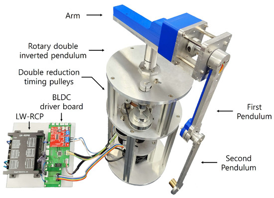
Figure 1. A rotary double inverted pendulum constructed in the laboratory.

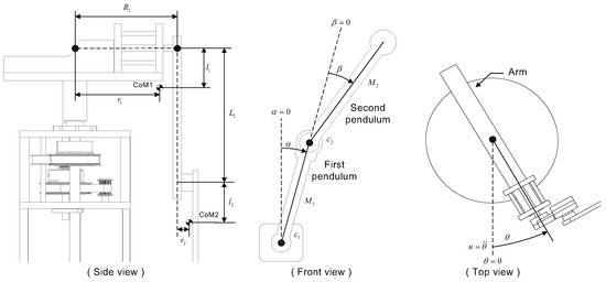
Figure 2. Conceptual diagram of a rotary double inverted pendulum.

2.1. Structure of the Rotary Double Inverted Pendulum

This paper uses the International System of Units (SI), and all variables and parameters are defined accordingly. Here, $\theta$ represents the arm’s rotational displacement from its initial position and u denotes its angular acceleration. CoM1 and CoM2 represent the centers of mass of the first and second pendulums, respectively. The distances $L_1$, $R_1$, $r_1$, $r_2$, $l_1$, and $l_2$ are illustrated in the side-view diagram of Figure 3. $M_1$ and $M_2$ denote the masses of the first and second pendulums, respectively. $\alpha$ is the rotational displacement of the first pendulum relative to the vertical ground normal, while $\beta$ represents the relative rotational displacement of the second pendulum with respect to the first pendulum. Furthermore, $c_1$ and $c_2$ denote the rotational friction coefficients at the pivots of the first and second pendulums, respectively. Figure 3 illustrates the inertia tensors I of the first and second pendulums. Terms such as $I_{xx1}$ and $I_{xx2}$ represent the moments of inertia along the x-axis for the first and second pendulums, respectively. Additionally, elements like $I_{xz1}$ and $I_{xz2}$ also represent components of the inertia tensor. Details of the gear reduction mechanism are shown in Figure 4.

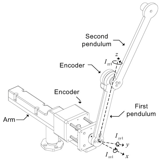
Figure 3. Inertia tensors of the first and second pendulums.

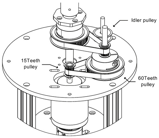
Figure 4. Double reduction structure of the rotary double inverted pendulum.

A BLDC motor is used as the drive component, and a double-reduction structure employing a timing belt and timing pulley is implemented to minimize backlash. By applying a 4:1 reduction ratio twice, a total reduction ratio of 16:1 is achieved, which improves the encoder resolution and enables precise angular velocity control. This structure is pivotal in enhancing the control performance of the rotary double inverted pendulum. First, the reduction mechanism minimizes backlash, reducing nonlinear effects. The high resolution of the encoder facilitates accurate dynamic modeling based on moments of inertia, reducing the discrepancy between control inputs and actual system responses and significantly improving model-based control consistency. Moreover, the dual-reduction structure ensures a stable high-torque output, effectively controlling the instability that can arise in nonlinear, multi-stage systems such as the rotary double inverted pendulum.

2.2. Mathematical Modeling of the Rotary Double Inverted Pendulum

The dynamic model of the rotary double inverted pendulum can be derived using the Euler–Lagrange equation as follows:

$$\begin{array}{c}\hfill \left[\begin{array}{c}{n}_1\\ n_2\end{array}\right]\ddot{\theta }+\left[\begin{array}{cc}{m}_{11}& m_{12}\\ m_{21}& m_{22}\end{array}\right]\left[\begin{array}{c}\ddot{\alpha }\\ \ddot{\beta }\end{array}\right]+\left[\begin{array}{c}{d}_1\\ d_2\end{array}\right]=0\end{array}$$

(1)

Each component of Equation (1) is defined as follows:

$$\begin{array}{cc}\hfill n_1& =h_{1}cos\left(\alpha \right)+h_{2}cos(\alpha +\beta ),\hfill \\ \hfill n_2& =h_{2}cos(\alpha +\beta ),\hfill \\ \hfill m_{11}& =h_3+h_6+2h_{4}cos\left(\beta \right),\hfill \\ \hfill m_{12}& =h_6+h_{4}cos\left(\beta \right),\hfill \\ \hfill m_{21}& =h_6+h_{4}cos\left(\beta \right),\hfill \\ \hfill m_{22}& =h_6,\hfill \\ \hfill d_1& =-h_{4}sin\beta (2\dot{\alpha }\dot{\beta }+{\dot{\beta }}^2)-h_{5}sin\alpha -h_{7}sin(\alpha +\beta )+c_1\dot{\alpha }\hfill \\ \hfill & -{\dot{\theta }}^2\{{\displaystyle \frac{1}{2}}{h}_{8}sin\left(2\alpha \right)+h_{4}sin(2\alpha +\beta )+{\displaystyle \frac{1}{2}}{h}_{9}sin(2\alpha +2\beta )\},\hfill \\ \hfill d_2& =h_{4}sin\beta \left({\dot{\alpha }}^2\right)-h_{7}sin(\alpha +\beta )+c_2\dot{\beta }\hfill \\ \hfill & -{\dot{\theta }}^2\{{\displaystyle \frac{1}{2}}{h}_{9}sin(2\alpha +2\beta )+{\displaystyle \frac{1}{2}}{h}_4(sin(2\alpha +2\beta )-sin\beta )\}.\hfill \end{array}$$

The terms $h_1-h_9$ are defined as follows, where g represents the gravitational acceleration of 9.81 [m/s²].

$$\begin{array}{ccc}\hfill h_1& =& M_1{l}_1{r}_1+M_2{L}_1(R_1+r_2)-I_{xz1},\hfill \\ \hfill h_2& =& M_2{l}_2(R_1+r_2)-I_{xz2},\hfill \\ \hfill h_3& =& I_{xx1}+M_1{l}_1^2+M_2{L}_1^2,\hfill \\ \hfill h_4& =& M_2{L}_1{l}_2,\hfill \\ \hfill h_5& =& g(M_1{l}_1+M_2{L}_1),\hfill \\ \hfill h_6& =& I_{xx2}+M_2{l}_2^2,\hfill \\ \hfill h_7& =& M_{2}g{l}_2,\hfill \\ \hfill h_8& =& M_1{l}_1^2+M_2{L}_1^2+I_{yy1}-I_{zz1},\hfill \\ \hfill h_9& =& M_2{l}_2^2+I_{yy2}-I_{zz2}.\hfill \end{array}$$

At this point, Equation (1) can be rearranged as follows:

$$\left[\begin{array}{c}\ddot{\alpha }\\ \ddot{\beta }\end{array}\right]=-{\left[\begin{array}{cc}{m}_{11}& m_{12}\\ m_{21}& m_{22}\end{array}\right]}^{-1}\left\{\left[\begin{array}{c}{n}_1\\ n_2\end{array}\right]\ddot{\theta }+\left[\begin{array}{c}{d}_1\\ d_2\end{array}\right]\right\}.$$

By solving this equation, we obtain

$$\begin{array}{ccc}\hfill \ddot{\alpha }& =& {\displaystyle \frac{(-m_{22}{n}_1+m_{12}{n}_2)\ddot{\theta }+(-m_{22}{d}_1+m_{12}{d}_2)}{\Phi }},\hfill \\ \hfill \ddot{\beta }& =& {\displaystyle \frac{(m_{21}{n}_1-m_{11}{n}_2)\ddot{\theta }+(m_{21}{d}_1-m_{11}{d}_2)}{\Phi }},\hfill \\ \hfill \Phi & =& m_{11}{m}_{22}-m_{12}{m}_{21}.\hfill \end{array}$$

Here, the state vector is defined as $x_1=\theta$, $x_2=\alpha$, $x_3=\beta$, $x_4=\dot{\theta }$, $x_5=\dot{\alpha }$, $x_6=\dot{\beta }$, and $x_7={\int }_0^t\theta \left(\tau \right)d\tau$, and the angular acceleration $\ddot{\theta }$ is represented as the control input u. The final model equations of the double inverted pendulum can be expressed as the following nonlinear state-space equations. Note that the last term of the state vector, ${\int }_0^t\theta \left(\tau \right)d\tau$, is added to eliminate the steady-state error of the arm’s position.

$$\underset{\dot{x}}{\underbrace{\left[\begin{array}{c}{\dot{x}}_1\\ {\dot{x}}_2\\ {\dot{x}}_3\\ {\dot{x}}_4\\ {\dot{x}}_5\\ {\dot{x}}_6\\ {\dot{x}}_7\end{array}\right]}}=\underset{f(x,u)}{\underbrace{\left[\begin{array}{c}{x}_4\\ x_5\\ x_6\\ u\\ {\displaystyle \frac{(-m_{22}{n}_1+m_{12}{n}_2)u+(-m_{22}{d}_1+m_{12}{d}_2)}{\Phi }}\\ {\displaystyle \frac{(m_{21}{n}_1-m_{11}{n}_2)u+(m_{21}{d}_1-m_{11}{d}_2)}{\Phi }}\\ x_1\end{array}\right]}}$$

(2)

The above-derived dynamic model is later used as the feedforward trajectory generation model when applying the direct collocation method.

2.3. Estimation of Physical Parameters of the Pendulum

To calculate the optimal state trajectory $x^{*}$ and control input trajectory $u^{*}$ required for transition control, we must accurately estimate the system parameters. Accordingly, parameters such as $M_1$, $M_2$, $I_{xx1}$, $I_{xx2}$, $I_{yy1}$, $I_{yy2}$, $I_{zz1}$, $I_{zz2}$, $I_{xz1}$, $I_{xz2}$, $l_1$, $l_2$, $c_1$, $c_2$, and $L_1$, as illustrated in Figure 2 and Figure 3, must be precisely estimated. Among these, $M_1$, $M_2$, $I_{xx1}$, $I_{xx2}$, $l_1$, $l_2$, $c_1$, and $c_2$ can be estimated using the parameter estimation method for the linear double inverted pendulum described in [23]. This method involves driving the arm of the rotary inverted pendulum in a specific manner and using the resulting state variable trajectories when the pendulums are oscillated. However, the values of the parameters that generate the measured state variable trajectories are not always unique. To better illustrate this, let us remove the second pendulum from the rotary double inverted pendulum. Then, the system reduces to a single inverted pendulum and its model equation can be expressed as follows:

$${\ddot{\theta }}_1={\zeta }_{1}sin{\theta }_1-{\zeta }_2{\dot{\theta }}_1-{\displaystyle \frac{{\zeta }_1}{g}}cos{\theta }_{1}u.$$

(3)

Here, ${\zeta }_1$ and ${\zeta }_2$ are defined as follows:

$${\zeta }_1={\displaystyle \frac{mg{l}_1}{I_{xx1}+m_1{l}_1^2}},{\zeta }_2={\displaystyle \frac{c_1}{I_{xx1}+m_1{l}_1^2}}.$$

(4)

Because ${\zeta }_1$ and ${\zeta }_2$ are functions of four parameters ($I_{xx1}$, $l_1$, $m_1$, and $c_1$), the combinations of $I_{xx1}$, $l_1$, $m_1$, and $c_1$ that produce the same ${\zeta }_1$ and ${\zeta }_2$ are not unique. However, if two of these parameters are fixed, a unique solution can be obtained to estimate the remaining parameters. Therefore, among the four parameters, $m_1$ and $l_1$ (which can be directly measured) are determined using a scale and a length-measuring device, respectively. The remaining parameters, $I_{xx1}$ and $c_1$, are estimated using experimental data. The parameters of the second pendulum are estimated using the same approach as the first pendulum. The inertia tensor can be estimated by using the method described in [7] or 3D modeling software to calculate the values. The parameters of the rotary double inverted pendulum obtained through this estimation and measurement are summarized as follows:

The transition control between the pendulum’s equilibrium points is performed using a 2-DOF control technique combining nonlinear feedforward control and feedback control, as proposed in [24]. Figure 5 illustrates the 2-DOF control structure. The precomputed ideal angular acceleration trajectory $u^{*}\left(t\right)$ is combined with the correction input $\Delta u\left(t\right)$, which is calculated based on the error $\Delta x\left(t\right)=x^{*}\left(t\right)-x\left(t\right)$ between the predicted and actual state variables of the inverted pendulum system. This generates the actual angular acceleration input $u\left(t\right)=u^{*}\left(t\right)+\Delta u\left(t\right)$. This control approach ensures smooth transitions between equilibrium points and improves the control system’s robustness by compensating for possible errors between the planned trajectory and the actual motion. In this paper, the feedforward trajectory is generated by considering the dynamic constraints and setting up a nonlinear optimal control problem that numerically minimizes the desired cost function while satisfying various constraints. The direct collocation method is used to numerically solve this problem [25]. This method effectively estimates the control inputs and state variable paths of continuous dynamic systems and is a proven technique for obtaining the optimal trajectory to achieve control objectives.

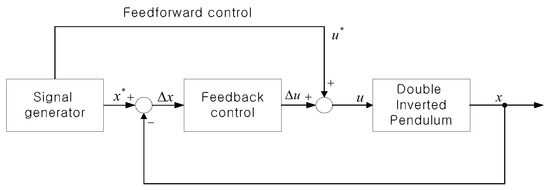
Figure 5. The 2-DOF control structure for the double inverted pendulum.

3. Transition Control

3.1. Design of Transition Control

The four equilibrium points of the rotary double inverted pendulum, determined by the states of the first and second pendulum segments, are illustrated in Figure 6. In this paper, the equilibrium points are defined by assigning the states “Up” and “Down” to 1 and 0, respectively, and representing them as binary numbers. Starting with the first pendulum segment, the equilibrium point where both the first and second segments are facing downward (Down–Down) corresponds to the binary number 00 and is labeled as EP0, while the equilibrium point corresponding to the Up–Down state is represented as 10 and labeled as EP2. This naming convention offers the advantage of assigning equilibrium points systematically according to the same binary rule, even when the number of pendulum segments increases. It also facilitates intuitive understanding of the pendulum’s equilibrium states. Henceforth, in this paper, the equilibrium points of the pendulum are denoted as EP0 (Down–Down), EP1 (Down–Up), EP2 (Up–Down), and EP3 (Up–Up).

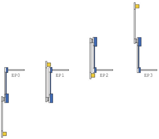
Figure 6. Four equilibrium points of a rotary double inverted pendulum.

Transition control is a complex problem that must satisfy both the stability of each equilibrium point and the transition process between them. To address this, the transition control follows three key steps. Each step is designed to ensure stability during the transition process, perform the transition operation, and maintain final stability.

• The linear control is performed to ensure the system’s stability at the current equilibrium point.
• The transition control is carried out to move from the current equilibrium point to the next.
• The linear control is performed to maintain stability at the next equilibrium point.

This structure is similar in principle to the swing-up problem, which involves moving the pendulum from the initial state (EP0) to the upright state (EP3). Therefore, the transition process must satisfy both stability and transition requirements at each step. In particular, the double inverted pendulum system has 12 distinct transition trajectories, making it essential to design and conduct experiments that satisfy the characteristics and conditions of each trajectory. The 12 transition trajectory paths proposed in this paper are constructed as shown in Figure 7.

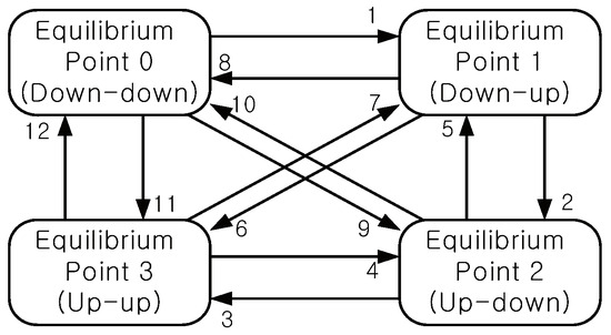
Figure 7. Twelve-step transition diagram of a double inverted pendulum.

3.2. Direct Collocation

The direct collocation method is an iterative numerical solution technique implemented using a nonlinear optimization solver. In this method, the shape of the initial trajectory provided by the designer can influence both the numerical solutions’ computation time and the resulting trajectory shape. By considering these characteristics, the designer can select an appropriate initial trajectory and apply direct collocation to derive a trajectory suitable for a specific transition control problem. In this paper, the initial trajectory is designed using the simplest form of a straight-line trajectory that connects the start and end boundary conditions. Additionally, a cost function is designed to satisfy all the specified constraints and boundary conditions, thereby formulating a general nonlinear optimal control problem. Equation (5) represents the optimal control problem formulated to compute the optimal trajectory.

$$\begin{array}{cc}\hfill \stackrel{\mathrm{Minimize}}{u\left(t\right)}& J\left(x\right(t),u(t\left)\right)\\ \hfill \mathrm{subject}\mathrm{to}& \mathrm{input}/\mathrm{output}\mathrm{constraint},& \\ \hfill & \mathrm{dynamic}\mathrm{equations},& \\ \hfill & \mathrm{boundary}\mathrm{conditions}.\end{array}$$

(5)

In the above equation, $J\left(x\right(t),u(t\left)\right)$ represents the cost function and is defined as an optimal control problem that satisfies the constraints established using the actual system model parameters listed in Table 1. The cost function can be used to minimize time or optimize the cost over a given time period. The constraints and limitations applied to the cost function include the dynamic equations of the rotary double inverted pendulum (2) and, as shown in (6), restrictions on the maximum arm rotation during the control process, as well as limitations on the arm’s maximum angular velocity and input angular acceleration within the actuator’s linear operating range. These conditions are crucial in ensuring the operational feasibility and stability of the control system.

$$\begin{array}{ccc}\hfill \left|x_1^{*}\right|\le {\theta }_{limit},& \left|{x_4}^{*}\right|\le {\dot{\theta }}_{limit},& \left|u^{*}\right|\le u_{limit}.\hfill \end{array}$$

(6)

Table 1. Summary of the parameters for the rotary double inverted pendulum.

Parameter	Value
$M_1$	0.187 kg
$M_2$	0.132 kg
$I_{xx1}$	1.0415$\times {10}^{-3}$ kgm2
$I_{xx2}$	8.8210$\times {10}^{-4}$ kgm2
$I_{yy1}$	4.3569$\times {10}^{-3}$ kgm2
$I_{yy2}$	4.9793$\times {10}^{-3}$ kgm2
$I_{zz1}$	3.3179$\times {10}^{-3}$ kgm2
$I_{zz2}$	4.8178$\times {10}^{-3}$ kgm2
$I_{xz1}$	3.7770$\times {10}^{-4}$ kgm2
$I_{xz2}$	1.9823$\times {10}^{-4}$ kgm2
$l_1$	0.072 m
$l_2$	0.133 m
$c_1$	2.4100$\times {10}^{-6}$
$c_2$	1.0900$\times {10}^{-6}$
$L_1$	0.1645 m
$R_1$	0.1625 m
$r_1$	0.1597 m
$r_2$	0.0209 m

The specified limits are all defined as positive values, with ${\theta }_{limit}>0$, ${\dot{\theta }}_{limit}>0$, and $u_{limit}>0$ representing the maximum allowable values for the arm’s output displacement, output angular velocity, and input angular acceleration, respectively. These limits reflect the actual operational constraints of the rotary double inverted pendulum used in the experiments, and the corresponding constraints are explicitly detailed in Table 2.

Table 2. Constraints for the experiment.

Transition Number	${\mathit{\theta }}_{\mathit{limit}}\left[\mathbf{rad}\right]$	${\dot{\mathit{\theta }}}_{\mathit{limit}}\left[\mathbf{rad}/\mathbf{s}\right]$	${\mathit{u}}_{\mathit{limit}}\left[{\mathbf{rad}/\mathbf{s}}^2\right]$
1	1.7	7.0	50
2	1.5	7.0	50
3	1.5	7.0	60
4	1.5	12	70
5	1.5	7.0	50
6	1.5	7.0	50
7	1.5	7.0	70
8	1.5	7.0	50
9	1.5	7.0	50
10	1.5	7.0	50
11	1.5	7.0	50
12	1.5	8.0	50

To satisfy various constraints in the 12 distinct transition control processes, additional constraints can also be applied to the pendulum’s rotational angles $\alpha$ and $\beta$, as well as their angular velocities $\dot{\alpha }$ and $\dot{\beta }$. Furthermore, at the start time ($t=0$) and end time ($t=T$) of the transition control, the boundary conditions corresponding to the equilibrium points for a specific transition must be satisfied. For instance, the starting and ending points differ depending on the transition number, and this situation is shown in Table 3.

Table 3. Boundary condition for 12 trajectories.

Transition Number	${\mathit{x}}^{*}\left(0\right)$	${\mathit{x}}^{*}\left(\mathit{T}\right)$
1	$\left[\begin{array}{c}0,-\pi ,0,0,0,0,0\end{array}\right]$	$\left[\begin{array}{c}0,-\pi ,-\pi ,0,0,0,0\end{array}\right]$
2	$\left[\begin{array}{c}0,-\pi ,-\pi ,0,0,0,0\end{array}\right]$	$\left[\begin{array}{c}0,0,-\pi ,0,0,0,0\end{array}\right]$
3	$\left[\begin{array}{c}0,0,-\pi ,0,0,0,0\end{array}\right]$	$\left[\begin{array}{c}0,2\pi ,0,0,0,0,0\end{array}\right]$
4	$\left[\begin{array}{c}0,0,0,0,0,0,0\end{array}\right]$	$\left[\begin{array}{c}0,0,-\pi ,0,0,0,0\end{array}\right]$
5	$\left[\begin{array}{c}0,0,-\pi ,0,0,0,0\end{array}\right]$	$\left[\begin{array}{c}0,-\pi ,-\pi ,0,0,0,0\end{array}\right]$
6	$\left[\begin{array}{c}0,-\pi ,-\pi ,0,0,0,0\end{array}\right]$	$\left[\begin{array}{c}0,0,0,0,0,0,0\end{array}\right]$
7	$\left[\begin{array}{c}0,0,0,0,0,0,0\end{array}\right]$	$\left[\begin{array}{c}0,-\pi ,-\pi ,0,0,0,0\end{array}\right]$
8	$\left[\begin{array}{c}0,-\pi ,-\pi ,0,0,0,0\end{array}\right]$	$\left[\begin{array}{c}0,-\pi ,0,0,0,0,0\end{array}\right]$
9	$\left[\begin{array}{c}0,-\pi ,0,0,0,0,0\end{array}\right]$	$\left[\begin{array}{c}0,0,-\pi ,0,0,0,0\end{array}\right]$
10	$\left[\begin{array}{c}0,0,-\pi ,0,0,0,0\end{array}\right]$	$\left[\begin{array}{c}0,-\pi ,0,0,0,0,0\end{array}\right]$
11	$\left[\begin{array}{c}0,-\pi ,0,0,0,0,0\end{array}\right]$	$\left[\begin{array}{c}0,0,0,0,0,0,0\end{array}\right]$
12	$\left[\begin{array}{c}0,0,0,0,0,0,0\end{array}\right]$	$\left[\begin{array}{c}0,-\pi ,0,0,0,0,0\end{array}\right]$

The transition trajectories obtained using the direct collocation method are shown in Figure 8 and Figure 9. Figure 8 illustrates the representative swing-up trajectory transitioning from EP0 to EP3, corresponding to transition 11. Figure 9 represents the control input trajectories used in all transitions. In the control input trajectories for transitions 4–7, the trajectories satisfy the prescribed constraints and boundary conditions during the transition process.

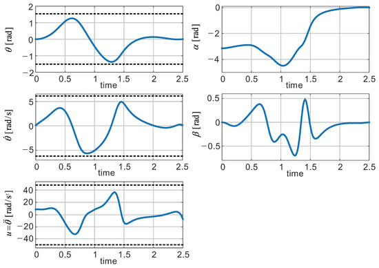
Figure 8. Feedforward transition trajectory from EP0 to EP3.

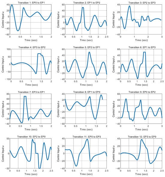
Figure 9. Feedforward transition trajectories for control input.

4. Experimental Results

4.1. Experimental Setup

The design of the feedback controller for trajectory tracking follows a similar approach to that of Graichen [24], as mentioned in the introduction, but with the distinction that this study applies the optimal LQ control technique for time-varying systems across the entire process. In Graichen’s research, the control system was shown to lose controllability due to high compensation values in regions where the gain coefficients increased sharply, leading to the decision to discontinue feedback in specific intervals. However, in this study, a consistent control strategy is maintained by utilizing the calculated time-varying LQ control gains throughout all intervals during transition control. This time-varying LQ controller utilizes a linearized dynamic system based on the swing-up trajectory of the double inverted pendulum system. The state equation, which varies over time and is used in this process, is modeled as a time-varying form of A and B values, as shown in Equation (7).

$$\begin{array}{ccc}\hfill A\left(t\right)={\left.{\displaystyle \frac{\partial f}{\partial x}}\right|}_{x^{*}\left(t\right),u^{*}\left(t\right)},& & B\left(t\right)={\left.{\displaystyle \frac{\partial f}{\partial u}}\right|}_{x^{*}\left(t\right),u^{*}\left(t\right)}.\hfill \end{array}$$

(7)

Here, $x^{*}\left(t\right)$ and $u^{*}\left(t\right)$ represent the feedforward trajectories for states and inputs obtained using the direct collocation method. The difference between the computed feedforward trajectory and the actual state variable values is calculated as $\Delta x\left(t\right)=x^{*}\left(t\right)-x\left(t\right)$, and the correction input $\Delta u\left(t\right)$, generated to compensate for this error, is defined by Equation (8):

$$\begin{array}{c}\hfill \Delta u\left(t\right)=-K\left(t\right)\Delta x\left(t\right).\end{array}$$

(8)

At this point, the time-varying state equation can be expressed as Equation (9):

$$\begin{array}{c}\hfill \Delta \dot{x}\left(t\right)=A\left(t\right)\Delta x\left(t\right)+B\left(t\right)\Delta u\left(t\right).\end{array}$$

(9)

The cost function is defined as follows:

$$\begin{array}{c}\hfill \begin{array}{cc}\hfill J& =\Delta x^T\left(T\right)H_{Tr}\Delta x\left(T\right)+{\int }_0^T\Delta x{\left(t\right)}^T{Q}_{Tr}\Delta x\left(t\right)+\Delta u{\left(t\right)}^T{R}_{Tr}\Delta u\left(t\right)dt.\end{array}\end{array}$$

(10)

Here, the subscript $Tr$ indicates the design variables for the transition process. In Equation (10), the variables with this subscript satisfy $H_{Tr}\ge 0$, $Q_{Tr}\ge 0$, and $R_{Tr}>0$. The matrix $H_{Tr}$ represents the weight on the terminal state, $Q_{Tr}$ represents the weight on the system state, and $R_{Tr}$ represents the weight on the control input. These weights are determined through experimental processes and are set to the following values:

$$\begin{array}{ccc}\hfill Q_{Tr}& =& \mathrm{diag}(1,300,500,1,1,1,1),\hfill \\ \hfill R_{Tr}& =& 1.\hfill \end{array}$$

(11)

In addition, the time-varying gain $K\left(t\right)$ must be calculated by solving the differential Riccati equation:

$$\begin{array}{c}\hfill \begin{array}{ccc}\hfill \dot{P}\left(t\right)& =& -A{\left(t\right)}^{T}P\left(t\right)-P\left(t\right)A\left(t\right)+P\left(t\right)B\left(t\right)R_{Tr}^{-1}{B}^T\left(t\right)P\left(t\right)-Q_{Tr},\hfill \\ \hfill P\left(T\right)& =& H_{Tr}.\hfill \end{array}\end{array}$$

(12)

Finally, the time-varying gain $K\left(t\right)$ can be computed using Equation (13). For example, the LQ control gain $K\left(t\right)$ applied in Figure 8 can be observed in Figure 10.

$$\begin{array}{c}\hfill K\left(t\right)=R_{Tr}^{-1}{B}^T\left(t\right)P\left(t\right).\end{array}$$

(13)

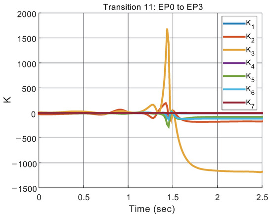
Figure 10. Time-varying LQ gain of feedforward transition trajectory from EP0 to EP3.

4.2. Experimental Data and Analysis

To conduct the experiments, 12 transition control types are implemented by combining the swing-up trajectory obtained using the direct collocation method presented in Section 3 with the feedback controller designed using LQ control. The transition sequences are structured according to Figure 7, and each transition sequence between equilibrium points is designed to be traversed only once. The duration of one cycle, which includes a state transition and linear control at an equilibrium point, is set to 5 s. The time required for state transitions varies from 1.8 s to 3 s, as shown in Table 4. During the time following each transition, linear control at the corresponding equilibrium point is performed to stabilize the system until the next transition control begins.

Table 4. Transition timing parameters used in the experiment.

Starting EP	Destination EP	T [s]
EP0	EP1	2.000
	EP2	3.000
	EP3	2.500
EP1	EP0	1.800
	EP2	2.500
	EP3	2.500
EP2	EP0	2.500
	EP1	2.000
	EP3	2.921
EP3	EP0	2.500
	EP1	2.000
	EP2	2.000

The first transition begins at the 5 s mark, and Figure 11 illustrates all transition control results sequentially. Solid lines represent the simulation model trajectories, and dotted lines show the measured closed-loop trajectory with compensation applied. Due to the compensation effect of closed-loop control, the arm’s rotation angle $\theta$ and angular velocity $\dot{\theta }$ exhibit significant differences immediately after the transition; however, through linear control at the equilibrium point, the $\theta$ value is gradually adjusted to approach zero. Additionally, the graphs for $\alpha$ and $\beta$, the most critical variables in transition control, demonstrate very precise tracking of the predicted trajectories. To further illustrate the experimental validation of the proposed method, a video of the experiments has been uploaded to YouTube. Figure 12 presents a screenshot of the video, and the full video can be accessed at the following link: https://youtu.be/J8vRJtQ-t3I, accessed on 15 January 2025. (video title: “12 transition controls of a rotary double inverted pendulum (with double reduction timing pulleys)”; channel name: Embedded Control Lab). This video visually demonstrates the transition control process, serving as a supplementary resource to the experimental results discussed in this section.

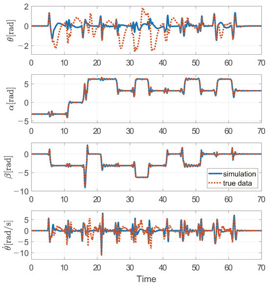
Figure 11. Twelve-step transition trajectories of a rotary double inverted pendulum: model trajectory (solid line) and actual trajectory (dotted line).

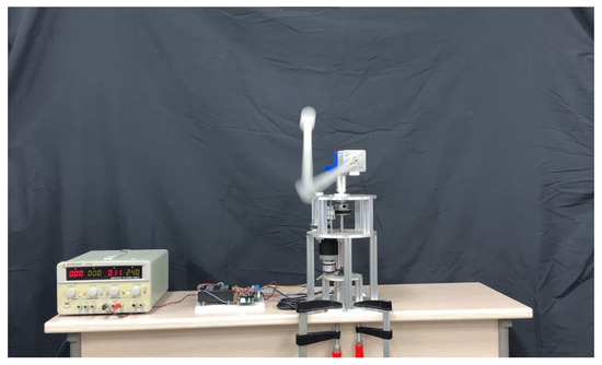
Figure 12. A YouTube video capture of the 12 transition controls of a rotary double inverted pendulum.

5. Conclusions

This study establishes an experimental environment using a lab-built rotary double inverted pendulum system and investigates 12 transition control problems, including swing-up control. For segmental transition control, the direct collocation method was introduced to generate feedforward trajectories, and a two-degree-of-freedom controller incorporating the designed time-varying LQ control implemented the 12 transition control paths. Finally, the proposed method’s efficiency and feasibility were demonstrated by sequentially controlling the 12 paths, which enables transitions among the four equilibrium points of the double inverted pendulum, over 60 s, with each path executed within 5 s.

The main contributions of this study are as follows: Firstly, it extends the conventional swing-up problem by defining and experimentally implementing transition control problems between equilibrium points. Secondly, it effectively addresses complex transition control problems by utilizing a two-degree-of-freedom control structure that integrates feedforward trajectory generation via the direct collocation method and time-varying LQ control. Lastly, the proposed method’s practicality is validated through experimental tests using a lab-built rotary double inverted pendulum system.

Building upon these contributions, future research could incorporate AI (artificial intelligence)-based techniques, such as reinforcement learning, to develop adaptive and robust control systems. By advancing the proposed approach and exploring its applicability to multidimensional and multi-actuator systems, this strategy could evolve into a universal control method for complex dynamic systems, further expanding its potential impact.

References

- Äström, K.J.; Furuta, K. Swinging up a pendulum by energy control. Automatica 2000, 36, 287–295. [Google Scholar] [CrossRef]
- Huang, S.; Huang, C. Control of an inverted pendulum using grey prediction model. IEEE Trans. Ind. Appl. 2000, 36, 452–458. [Google Scholar] [CrossRef]
- Otani, Y.; Kurokami, T.; Inoue, A.; Hirashima, Y. A Swingup Control of an Inverted Pendulum with Cart Position Control. In Proceedings of the IFAC Conference on New Technologies for Computer Control (NTCC 2001), Hong Kong, China, 19–22 November 2001; pp. 395–400. [Google Scholar]
- Muskinja, N.; Tovornik, B. Swinging up and stabilization of a real inverted pendulum. IEEE Trans. Ind. Electron. 2006, 53, 631–639. [Google Scholar] [CrossRef]
- Äström, K.J.; Aracil, J.; Gordillo, F. A family of smooth controllers for swinging up a pendulum. Automatica 2008, 44, 1841–1848. [Google Scholar] [CrossRef][Green Version]
- Erwin, S.; Agung, S.W.; Elvandry, G.R. Fuzzy Swing Up Control and Optimal State Feedback Stabilization for Self-Erecting Inverted Pendulum. IEEE Access 2020, 8, 6496–6504. [Google Scholar]
- Oh, Y.; Lee, Y.S. Robust Swing-up Control of a Rotary Inverted Pendulum Subject to Input/Output Constraints. J. Inst. Control. Robot. Syst. 2018, 24, 423–430. [Google Scholar] [CrossRef]
- Ratiroch-Anant, P.; Anabuki, M.; Hirata, H. Self-tuning control for rotational inverted pendulum by: Eigenvalue approach. In Proceedings of the IEEE Region 10 Conference TENCON 2004, Chiang Mai, Thailand, 21–24 November 2004; pp. 542–545. [Google Scholar]
- Rahairi, M.R.; Selamat, H.; Zamzuri, H.; Ahmad, F. PID controller optimization for a rotational inverted pendulum using genetic algorithm. In Proceedings of the 2011 Fourth International Conference on Modeling, Simulation and Applied Optimization, Kuala Lumpur, Malaysia, 19–21 April 2011; pp. 1–6. [Google Scholar]
- Thein, M.-W.L.; Misawa, E.A. Comparison of the sliding observer to several state estimators using a rotational inverted pendulum. In Proceedings of the 1995 34th IEEE Conference on Decision and Control, New Orleans, LA, USA, 13–15 December 1995; pp. 3385–3390. [Google Scholar]
- Brown, D.; Strube, M. Design of a Neural Controller Using Reinforcement Learning to Control a Rotational Inverted Pendulum. In Proceedings of the 2020 21st International Conference on Research and Education in Mechatronics (REM), Cracow, Poland, 9–11 December 2020; pp. 1–5. [Google Scholar]
- Hernandez, R.; Garcia-Hernandez, R.; Jurado, F. Modeling, Simulation, and Control of a Rotary Inverted Pendulum: A Reinforcement Learning-Based Control Approach. Modelling 2024, 5, 1824–1852. [Google Scholar] [CrossRef]
- Cherrat, N.; Hamid, B.; Hichem, A.; Ratiba, F. Experimental Study of Swing-Up PD and Sliding Mode Control for Rotary Inverted Pendulum. In Proceedings of the 2024 3rd International Conference on Advanced Electrical Engineering (ICAEE), Sidi-Bel-Abbes, Algeria, 5–7 November 2024. [Google Scholar]
- Jensen, J.N.; Ishizaki, T. Furuta Pendulum Design Update for Accessible Control Demonstrations. IFAC-PapersOnLine 2023, 56, 7573–7578. [Google Scholar] [CrossRef]
- Liang, F.; Xin, X.; Li, Y. Swing-up and Balance Control of Rotary Double Inverted Pendulum. In Proceedings of the 2023 3rd International Conference on Robotics and Control Engineering, Nanjing, China, 12–14 May 2023; pp. 65–70. [Google Scholar]
- Tran, N.; Nguyen, V.; Le, C.; Lai, A.; Nguyen, T.; Huynh, M.; Phan, V.; Tong, G.; Nguyen, L.; Ngo, T. LQR Control for Experimental Double Rotary Inverted Pendulum. J. Fuzzy Syst. Control. 2024, 2, 104–108. [Google Scholar]
- Singh, S.; Swarup, A. Control of Rotary Double Inverted Pendulum using Sliding Mode Controller. In Proceedings of the 2021 International Conference on Intelligent Technologies (CONIT), Hubli, India, 27 June 2021; pp. 1–6. [Google Scholar]
- Zied, B.H.; Mohammad, J.F.; Zafer, B. Development of a Fuzzy-LQR and Fuzzy-LQG stability control for a double link rotary inverted pendulum. J. Frankl. Inst. 2020, 357, 10529–10556. [Google Scholar]
- Ibrahim, M.M.; Ubaid, M.A.; Rachid, M.; Maamar, B. Stabilization of a double inverted rotary pendulum through fractional order integral control scheme. Int. J. Adv. Robot. Syst. 2019, 16, 4. [Google Scholar]
- Sondarangallage, D.A.; Manukid, P. Control of rotary double inverted pendulum system using mixed sensitivity H∞ controller. Int. J. Adv. Robot. Syst. 2019, 16, 2. [Google Scholar]
- Quanser Official Home Page. Available online: www.quanser.com (accessed on 8 January 2025).
- Sondarangallage, D.A.; Manukid, P. Control of rotary double inverted pendulum system using LQR sliding surface based sliding mode controller. J. Control Decis. 2022, 9, 89–101. [Google Scholar]
- Ju, D.; Choi, C.; Jeong, J.; Lee, Y.S. Design and parameter estimation of a double inverted pendulum for model-based swing-up control. J. Inst. Control. Robot. Syst. 2022, 28, 793–803. [Google Scholar] [CrossRef]
- Graichen, K.; Treuer, M.; Zeitz, M. Swing-up of the double pendulum on a cart by feedforward and feedback control with experimental validation. Automatica 2007, 43, 63–71. [Google Scholar] [CrossRef]
- Kelly, M. An introduction to trajectory optimization: How to do your own direct collcation. SIAM Rev. 2017, 59, 849–904. [Google Scholar] [CrossRef]
- Ju, D.; Lee, T.; Lee, Y.S. Implementation of 12 Transition Controls for Rotary Double Inverted Pendulum Using Direct Collocation. In Proceedings of the ICINCO 2024, Portu, Portugal, 18–20 November 2024. [Google Scholar]
- Lee, Y.S.; Jo, B.; Han, S. A light-weight rapid control prototyping system based on open source hardware. IEEE Access 2017, 5, 11118–11130. [Google Scholar] [CrossRef]
Disclaimer/Publisher’s Note: The statements, opinions and data contained in all publications are solely those of the individual author(s) and contributor(s) and not of MDPI and/or the editor(s). MDPI and/or the editor(s) disclaim responsibility for any injury to people or property resulting from any ideas, methods, instructions or products referred to in the content. |
© 2025 by the authors. Licensee MDPI, Basel, Switzerland. This article is an open access article distributed under the terms and conditions of the Creative Commons Attribution (CC BY) license (https://creativecommons.org/licenses/by/4.0/).