Internality of Two-Measure-Based Generalized Gauss Quadrature Rules for Modified Chebyshev Measures II

Abstract

Gaussian quadrature rules are commonly used to approximate integrals with respect to a non-negative measure $d\widehat{\sigma }$. It is important to be able to estimate the quadrature error in the Gaussian rule used. A common approach to estimating this error is to evaluate another quadrature rule that has more nodes and higher algebraic degree of precision than the Gaussian rule, and use the difference between this rule and the Gaussian rule as an estimate for the error in the latter. This paper considers the situation when $d\widehat{\sigma }$ is a Chebyshev measure that is modified by a linear factor and a linear divisor, and investigates whether the rules in a recently proposed new class of quadrature rules for estimating the error in Gaussian rules are internal, i.e., if all nodes of the new quadrature rules are in the interval $(-1,1)$. These new rules are defined by two measures, one of which is a modified Chebyshev measure $d\widehat{\sigma }$. The other measure is auxiliary.

1. Introduction

It is a common task in scientific computing to calculate approximations of integrals of the form

$$I\left(f\right)={\int }_{-1}^{1}f\left(x\right)d\widehat{\sigma }\left(x\right),$$

(1)

where $d\widehat{\sigma }$ is a non-negative measure and f is a real-valued integrand. A standard approach to evaluating such approximations when the coefficients of the recursion formula for the monic orthogonal polynomials that are associated with the measure $d\widehat{\sigma }$ are known or easily computable is to apply an ℓ-node Gaussian quadrature rule $G_{\mathcal{\ell }}\left(f\right)$$\left(={\sum }_{k=1}^{\mathcal{\ell }}{\omega }_k^{G}f\left(x_k^G\right)\right)$ associated with the measure $d\widehat{\sigma }$. A reason for the popularity of Gaussian quadrature rules is that they have maximal algebraic degree of precision: the Gaussian rule $G_{\mathcal{\ell }}$ has algebraic degree of precision $2\mathcal{\ell }-1$, which is maximal for all quadrature rules with ℓ nodes. Thus

$$I\left(f\right)=G_{\mathcal{\ell }}\left(f\right),\forall f\in {\mathbb{P}}_{2\mathcal{\ell }-1},$$

where ${\mathbb{P}}_{2\mathcal{\ell }-1}$ denotes the set of all polynomials of degree of at most $2\mathcal{\ell }-1$; see, e.g., [1,2,3,4,5] for details, including many applications as well as software.

It is important to be able to estimate the quadrature error

$$I\left(f\right)-G_{\mathcal{\ell }}\left(f\right)$$

(2)

so that a suitable value of the number of nodes, ℓ, can be chosen. We would like to choose the number of nodes ℓ large enough so that the error (2) is smaller than a specified tolerance, but we do not want ℓ to be unnecessarily large, since this would entail the evaluation of the integrand at a needlessly high number of nodes.

A standard approach to estimating the quadrature error (2) is to apply another quadrature rule, $Q_m\left(f\right)$, with $m>\mathcal{\ell }$ nodes, with higher algebraic degree of precision than $G_{\mathcal{\ell }}$, and using the difference $Q_m\left(f\right)-G_{\mathcal{\ell }}\left(f\right)$ as an estimate for the quadrature error (2). This paper analyzes the properties of a new class of quadrature rules $Q_m$.

We consider the situation when the measure $d\widehat{\sigma }$ in (1) is a Chebyshev measure that has been modified by a linear factor and a linear divisor, i.e.,

$$d\widehat{\sigma }\left(x\right)={\displaystyle \frac{x+\gamma }{x+\delta }}{(1-x)}^{\mp 1/2}{(1+x)}^{\mp 1/2}dx,-1<x<1,$$

(3)

where the parameters $\gamma$ and $\delta$ are given by

$$\gamma ={\displaystyle \frac{1}{2}}(v+v^{-1})\mathrm{and}\delta ={\displaystyle \frac{1}{2}}(u+u^{-1})$$

(4)

for some constants $u,v\in (-1,1)$. Clearly, $\gamma \ne \delta$ implies that $u\ne v$. We will consider “comparison quadrature rules” $Q_m$ that are constructed with the aid of two measures, a modified Chebyshev measure $d\widehat{\sigma }$ and an auxiliary measure $d\mu$ that also is defined on the interval $(-1,1)$. These kinds of two-measure-based quadrature rules were recently introduced in [6] and have been further studied in [7]. In these references, these rules were referred to as new averaged Gaussian (NAG) rules. We will use this acronym in the present paper also.

It is the purpose of this paper to investigate whether NAG quadrature rules ${\widehat{Q}}_{2\mathcal{\ell }+1}$ that are associated with a modified Chebyshev measure of the form (3) and an auxiliary measure $d\mu$ are internal, i.e., whether all nodes of ${\widehat{Q}}_{2\mathcal{\ell }+1}$ live in the interval $(-1,1)$. This property is important when approximating integrals (1) with an integrand f that is defined only in the interval $(-1,1)$.

The classical approach to estimating the quadrature error in an ℓ-node Gaussian rule $G_{\mathcal{\ell }}$ is to evaluate an associated $(2\mathcal{\ell }+1)$-node Gauss–Kronrod rule; see Gautschi [3] as well as [8,9,10,11,12,13] for discussions on properties and applications of Gauss–Kronrod rules. Our interest in NAG rules stems from the fact that they are much easier to compute; see [14,15] for algorithms for computing Gauss–Kronrod rules. The evaluation of NAG rules will be discussed below.

Another approach to estimating the quadrature error in $G_{\mathcal{\ell }}$ is to let the rule $Q_m$ be the averaged rule, denoted by $Q_{2\mathcal{\ell }+1}^L$, associated with $G_{\mathcal{\ell }}$. This averaged rule is the average of $G_{\mathcal{\ell }}$ and the associated $(\mathcal{\ell }+1)$-node anti-Gauss rule $G_{\mathcal{\ell }+1}^{\prime }$. Also, the averaged rule is much easier to compute than the Gauss–Kronrod rule associated with $G_{\mathcal{\ell }}$. Both anti-Gauss and averaged rules were introduced by Laurie [16]. More details on these rules will be provided below. For now, it suffices to note that they are not internal for all modified Chebyshev measures (3), and this is the reason for our interest in investigating whether certain NAG rules defined below are internal.

Spalević [17] (following Peherstorfer’s results; see [18,19]) proposed a variant of the averaged rule of Laurie [16] and referred to it as a generalized averaged rule. We will denote the generalized averaged rule associated with $G_{\mathcal{\ell }}$ as $Q_{2\mathcal{\ell }+1}^S$; it has $2\mathcal{\ell }+1$ nodes, similarly to the averaged rule $Q_{2\mathcal{\ell }+1}^L$ introduced by Laurie, and, generally, has higher degree of algebraic precision. However, these rules are not internal for all modified Chebyshev measures (3) either. Their computation is discussed in [20,21,22].

It is convenient to write the measures (3) in the form

$$d\widehat{\sigma }\left(x\right)={\displaystyle \frac{x+\gamma }{x+\delta }}d\sigma \left(x\right),-1<x<1,$$

(5)

and to define the measures

$$d\tilde{\sigma }\left(x\right)={\displaystyle \frac{1}{x+\delta }}d\sigma \left(x\right),$$

where $d\sigma$ is one of the four Chebyshev measures,

$$d\sigma \left(x\right)={(1-x)}^{\mp 1/2}{(1+x)}^{\mp 1/2}dx.$$

Given monic orthogonal polynomials $P_k$ and their recurrence coefficients ${\alpha }_k$ and ${\beta }_k$ for one of the measures $d\sigma$, Gautschi [3] [Section 2.4] describes algorithms for computing monic orthogonal polynomials ${\tilde{P}}_k$ and their recurrence coefficients ${\tilde{\alpha }}_k$ and ${\tilde{\beta }}_k$ for the measure $d\tilde{\sigma }$, as well as monic orthogonal polynomials ${\widehat{P}}_k$ and their recurrence coefficients ${\widehat{\alpha }}_k$ and ${\widehat{\beta }}_k$ for the measure $d\widehat{\sigma }$. The averaged Gaussian quadrature rules $Q_{2\mathcal{\ell }+1}^L$ and the generalized averaged Gaussian quadrature rules $Q_{2\mathcal{\ell }+1}^S$ coincide with the $(2\mathcal{\ell }+1)$-node Gauss–Kronrod quadrature rule for the measures $d\tilde{\sigma }$ for $\mathcal{\ell }\ge 3$ and are internal; see [23,24,25]. This paper therefore considers generalized averaged Gaussian quadrature rules for the measure $d\widehat{\sigma }$.

Averaged and generalized averaged quadrature rules are applicable to all integrands that are defined and continuous only within the interval $[-1,1]$ if they are internal. Djukić et al. [26] discuss two approaches to determining modifications of generalized averaged Gaussian quadrature rules with nodes in $[-1,1]$ when the generalized averaged rule is not internal: (i) truncating the Jacobi matrix associated with the generalized averaged Gaussian quadrature rule and (ii) weighting the generalized averaged Gaussian quadrature rule. Djukić et al. [26] also investigate the internality of averaged and generalized averaged quadrature rules, and truncated variants of the latter, for the measures (5) and show that weighting yields internal generalized averaged rules if a weighting parameter is chosen properly. Bounds for this parameter that guarantee internality are provided.

This paper considers NAG quadrature rules ${\widehat{Q}}_{2\mathcal{\ell }+1}$ that are determined by the measure $d\widehat{\sigma }$ as well as by an auxiliary measure $d\mu$. We will apply these rules to estimate the error in Gaussian quadrature rules. The purpose of the auxiliary measure $d\mu$ is to help define an internal quadrature rule with higher degree of algebraic precision than the associated Gaussian rule. NAG quadrature rules are attractive to use for estimating the error in Gaussian rules with respect to the measures $d\widehat{\sigma }$ when the averaged and generalized averaged Gaussian rules are not internal. An advantage of the NAG rules ${\widehat{Q}}_{2\mathcal{\ell }+1}$ relative to the corresponding weighted generalized averaged Gaussian quadrature rules is that the algebraic degree of precision of ${\widehat{Q}}_{2\mathcal{\ell }+1}$ is $2\mathcal{\ell }+2$, while the algebraic degree of precision of the corresponding weighted generalized averaged Gaussian quadrature rules only is $2\mathcal{\ell }+1$; see [6].

Let ${\tilde{p}}_k$, $k=0,1,2,\dots$, denote the monic orthogonal polynomials for the measure $d\mu$, and let ${\gamma }_k$ and ${\delta }_k$ be the coefficients of their three-term recurrence relation. It is shown in [6] that the nodes of the NAG quadrature rule ${\widehat{Q}}_{2\mathcal{\ell }+1}$ are the zeros of the polynomial

$$t_{2\mathcal{\ell }+1}={\tilde{p}}_{\mathcal{\ell }}·{\widehat{P}}_{\mathcal{\ell }+1}-{\widehat{\beta }}_{\mathcal{\ell }+1}{\tilde{p}}_{\mathcal{\ell }-1}·{\widehat{P}}_{\mathcal{\ell }}.$$

(6)

Let $J_{2\mathcal{\ell }+1}(d\widehat{\sigma },d\mu )\in {\mathbb{R}}^{(2\mathcal{\ell }+1)\times (2\mathcal{\ell }+1)}$ be the symmetric tridiagonal Jacobi matrix associated with the NAG rule ${\widehat{Q}}_{2\mathcal{\ell }+1}$. It has the entries

$$\left[\begin{array}{ccccccccc}{\widehat{\alpha }}_0& \sqrt{{\widehat{\beta }}_1}& & & & & & & 0\\ \sqrt{{\widehat{\beta }}_1}& {\widehat{\alpha }}_1& \sqrt{{\widehat{\beta }}_2}& & \\ & \ddots & \ddots & \ddots & \\ & & \sqrt{{\widehat{\beta }}_{\mathcal{\ell }-1}}& {\widehat{\alpha }}_{\mathcal{\ell }-1}& \sqrt{{\widehat{\beta }}_{\mathcal{\ell }}}\\ & & & \sqrt{{\widehat{\beta }}_{\mathcal{\ell }}}& {\widehat{\alpha }}_{\mathcal{\ell }}& \boxed{\sqrt{{\widehat{\beta }}_{\mathcal{\ell }+1}}}\\ & & & & \boxed{\sqrt{{\widehat{\beta }}_{\mathcal{\ell }+1}}}& {\gamma }_{\mathcal{\ell }-1}& \sqrt{{\delta }_{\mathcal{\ell }-1}}\\ & & & & & \sqrt{{\delta }_{\mathcal{\ell }-1}}& {\gamma }_{\mathcal{\ell }-2}& \ddots \\ & & & & & \ddots & \ddots & & \\ & & & & & & & {\gamma }_1& \sqrt{{\delta }_1}\\ 0& & & & & & & \sqrt{{\delta }_1}& {\gamma }_0\end{array}\right],$$

(7)

where we circumscribe the last entries that are determined by the measure $d\sigma$ by rectangles. The nodes and weights can be conveniently evaluated in $\mathcal{O}\left({\mathcal{\ell }}^2\right)$ arithmetic floating point operations by means of either the Golub–Welsch algorithm or a divide-and-conquer method; see [20,21,27]. The nodes and weights of the Gaussian rule $G_{\mathcal{\ell }}$ can be determined by applying the Golub–Welsch algorithm or a divide-and-conquer method to the leading principal $\mathcal{\ell }\times \mathcal{\ell }$ submatrix of (7). Computed examples reported in [20,21] illustrate that a divide-and-conquer method may yield higher accuracy and require less CPU-time for computing the nodes and weights of the quadrature rules $G_{\mathcal{\ell }}$ and ${\widehat{Q}}_{2\mathcal{\ell }+1}$ than available implementations of the Golub–Welsch algorithm.

In this paper, we consider NAG rules ${\widehat{Q}}_{2\mathcal{\ell }+1}$ with the auxiliary measure $d\mu$ chosen to be the Chebyshev measure of the second kind

$$d\mu \left(x\right)=\sqrt{1-x^2}dx,-1\le x\le 1;$$

see [6] [Remark 5.3]. Then, ${\gamma }_k=0,k=0,1,2,\cdots$, ${\delta }_0=\pi /2$, ${\delta }_k=1/4,k=1,2,3,\cdots$ The Jacobi matrix (7) is then of the form

$$\left[\begin{array}{ccccccccc}{\widehat{\alpha }}_0& \sqrt{{\widehat{\beta }}_1}& & & & & & & 0\\ \sqrt{{\widehat{\beta }}_1}& {\widehat{\alpha }}_1& \sqrt{{\widehat{\beta }}_2}& & \\ & \ddots & \ddots & \ddots & \\ & & \sqrt{{\widehat{\beta }}_{\mathcal{\ell }-1}}& {\widehat{\alpha }}_{\mathcal{\ell }-1}& \sqrt{{\widehat{\beta }}_{\mathcal{\ell }}}\\ & & & \sqrt{{\widehat{\beta }}_{\mathcal{\ell }}}& {\widehat{\alpha }}_{\mathcal{\ell }}& \boxed{\sqrt{{\widehat{\beta }}_{\mathcal{\ell }+1}}}\\ & & & & \boxed{\sqrt{{\widehat{\beta }}_{\mathcal{\ell }+1}}}& 0& \sqrt{{\displaystyle \frac{1}{4}}}\\ & & & & & \sqrt{{\displaystyle \frac{1}{4}}}& 0& \ddots \\ & & & & & \ddots & \ddots & & \\ & & & & & & & 0& \sqrt{{\displaystyle \frac{1}{4}}}\\ 0& & & & & & & \sqrt{{\displaystyle \frac{1}{4}}}& 0\end{array}\right].$$

(8)

The orthogonal polynomials ${\tilde{p}}_k$ are monic Chebyshev polynomials of the second kind ${\stackrel{\circ }{U}}_k=U_k/2^k$, where

$$U_k\left(x\right)={\displaystyle \frac{sin\left(\right(k+1\left)\theta \right)}{sin\left(\theta \right)}},x=cos\left(\theta \right),-\pi <\theta <\pi .$$

Formula (6) becomes

$$t_{2\mathcal{\ell }+1}={\stackrel{\circ }{U}}_{\mathcal{\ell }}·{\widehat{P}}_{\mathcal{\ell }+1}-{\widehat{\beta }}_{\mathcal{\ell }+1}{\stackrel{\circ }{U}}_{\mathcal{\ell }-1}·{\widehat{P}}_{\mathcal{\ell }}.$$

(9)

These formulas for the particular case of measures (5), when

$$\gamma =-\left({\displaystyle \frac{1}{2}}c+c^{-1}\right),\delta =-{\displaystyle \frac{1}{2}}\left(c+c^{-1}\right),$$

and $c\in \mathbb{R}\setminus \{-1,0\}$, were recently discussed in [7].

2. Internality of the Quadrature Rules ${\widehat{Q}}_{2\mathcal{\ell }+1}$ Determined by Modified Chebyshev Measures of the First Kind

Consider the Chebyshev measure of the first kind,

$$d\sigma \left(x\right)={\displaystyle \frac{dx}{\sqrt{1-x^2}}}.$$

Then the measure (5) is of the form

$$d\widehat{\sigma }\left(x\right)=d{\widehat{\sigma }}_1\left(x\right)={\displaystyle \frac{x+\gamma }{x+\delta }}{\displaystyle \frac{dx}{\sqrt{1-x^2}}},x\in (-1,1),$$

(10)

We recall some formulas that are discussed by Gautschi [3] [Section 2.4] and in [26]. First note that

$$\delta >1,u\in (0,1);v\in (-1,1),\gamma \in (-\infty ,-1)\cup (1,+\infty ),$$

so that $1+\gamma <0$, when $\gamma \in (-\infty ,-1)$, while $-1+\gamma >0$, when $\gamma \in (1,+\infty )$. Furthermore,

$${\tilde{P}}_k\left(x\right)={\displaystyle \frac{1}{2^{k-1}}}(T_k\left(x\right)+u{T}_{k-1}\left(x\right)),k\ge 2,$$

with ${\tilde{P}}_0\left(x\right)\equiv 1$ and ${\tilde{P}}_1\left(x\right)=x+u$. Here, $T_k$ denotes the Chebyshev polynomial of the first kind of degree k defined by

$$T_k\left(x\right)=cos\left(k\theta \right),x=cos\left(\theta \right).$$

(11)

The coefficients of the three-term recursion formula for the polynomials ${\tilde{P}}_k$ are

$$\begin{array}{ccc}\hfill {\tilde{\alpha }}_0& =& -u,{\tilde{\alpha }}_1={\displaystyle \frac{1}{2}}u,{\tilde{\alpha }}_k=0\mathrm{for}k\ge 2,\hfill \\ \hfill {\tilde{\beta }}_0& =& {\displaystyle \frac{2\pi u}{1-u^2}},{\tilde{\beta }}_1={\displaystyle \frac{1}{2}}(1-u^2),{\tilde{\beta }}_k={\displaystyle \frac{1}{4}}\mathrm{for}k\ge 2.\hfill \end{array}$$

Moreover, we have

$${\widehat{P}}_k\left(x\right)={\displaystyle \frac{{\tilde{P}}_{k+1}\left(x\right)-r_k{\tilde{P}}_k\left(x\right)}{x+\gamma }},$$

(12)

where

$$r_k={\displaystyle \frac{{\tilde{P}}_{k+1}(-\gamma )}{{\tilde{P}}_k(-\gamma )}},{\tilde{P}}_k(-\gamma )\ne 0.$$

(13)

The coefficients of the three-term recurrence relation for the polynomials ${\widehat{P}}_k$ are given by

$$\begin{array}{cc}\hfill {\widehat{\alpha }}_k=& {\tilde{\alpha }}_{k+1}+r_{k+1}-r_k,k\ge 0,\hfill \\ \hfill {\widehat{\beta }}_0=& -r_0{\tilde{\beta }}_0,{\widehat{\beta }}_k={\tilde{\beta }}_k{r}_k/r_{k-1},k\ge 1.\hfill \end{array}$$

(14)

For the coefficients $r_k$, one has

$$r_0=u-{\displaystyle \frac{1}{2}}(v+v^{-1}),r_k=-{\displaystyle \frac{1}{2v}}{\displaystyle \frac{v^{2k+1}-A}{v^{2k-1}-A}},k\ge 1,$$

where

$$A={\displaystyle \frac{1-uv}{u-v}};\left|A\right|>1,\mathrm{sgn}\left(A\right)=\mathrm{sgn}(u-v).$$

We note that $v>u$ is equivalent to $\delta >\gamma >1$, and $v(v-u)>0$ is equivalent to $\delta >\gamma$; see [26] for details.

The following cases have to be considered:

• $v>u$, which is equivalent to $\delta >\gamma >1$ ($A<-1$); $1+\gamma >0$.
• $0<v<u$, what is equivalent to $\delta <\gamma$ ($A>1$); $1+\gamma >0$.
• $-1<v<0<u$, what is equivalent to $\delta >\gamma (<-1)$ ($A>1$); $1+\gamma <0$.

It is shown in [26] [Theorem 3.2] that the averaged Gaussian quadrature rule $Q_{2\mathcal{\ell }+1}^L$ has an external node for every $\mathcal{\ell }\ge 1$, and it is demonstrated in [26] [Theorem 3.3] that the generalized averaged Gaussian quadrature rule $Q_{2\mathcal{\ell }+1}^S$ is internal if and only if $\delta >\gamma$. These properties suggest that NAG rules $Q_{2\mathcal{\ell }+1}$ should be developed for the case $\gamma <\delta$. If ${\widehat{Q}}_{2\mathcal{\ell }+1}$ is internal, then it may be used as an alternative to the quadrature rules $Q_{2\mathcal{\ell }+1}^L$ and $Q_{2\mathcal{\ell }+1}^S$ when the integrand is not defined outside the interval $(-1.1)$.

Using the above formulas, we obtain from (9) that

$$t_{2\mathcal{\ell }+1}\left(x\right)={\displaystyle \frac{{\tilde{P}}_{\mathcal{\ell }+2}\left(x\right)-r_{\mathcal{\ell }+1}{\tilde{P}}_{\mathcal{\ell }+1}\left(x\right)}{x+\gamma }}{\stackrel{\circ }{U}}_{\mathcal{\ell }}\left(x\right)-{\widehat{\beta }}_{\mathcal{\ell }+1}-{\displaystyle \frac{{\tilde{P}}_{\mathcal{\ell }+1}\left(x\right)-r_{\mathcal{\ell }}{\tilde{P}}_{\mathcal{\ell }}\left(x\right)}{x+\gamma }}{\stackrel{\circ }{U}}_{\mathcal{\ell }-1}\left(x\right),$$

(15)

i.e.,

$$\begin{array}{ccc}\hfill t_{2\mathcal{\ell }+1}\left(x\right)& =& {\displaystyle \frac{{\displaystyle \frac{1}{2^{\mathcal{\ell }+1}}(T_{\mathcal{\ell }+2}\left(x\right)+u{T}_{\mathcal{\ell }+1}\left(x\right))-r_{\mathcal{\ell }+1}\frac{1}{2^{\mathcal{\ell }}}(T_{\mathcal{\ell }+1}\left(x\right)+u{T}_{\mathcal{\ell }}\left(x\right))}}{x+\gamma }{\stackrel{\circ }{U}}_{\mathcal{\ell }}\left(x\right)}\hfill \\ & -& {\widehat{\beta }}_{\mathcal{\ell }+1}{\displaystyle \frac{{\displaystyle \frac{1}{2^{\mathcal{\ell }}}(T_{\mathcal{\ell }+1}\left(x\right)+u{T}_{\mathcal{\ell }}\left(x\right))-r_{\mathcal{\ell }}\frac{1}{2^{\mathcal{\ell }-1}}(T_{\mathcal{\ell }}\left(x\right)+u{T}_{\mathcal{\ell }-1}\left(x\right))}}{x+\gamma }}{\stackrel{\circ }{U}}_{\mathcal{\ell }-1}\left(x\right).\hfill \end{array}$$

In order for the largest node of the quadrature rule ${\widehat{Q}}_{2\mathcal{\ell }+1}$ to be smaller than or equal to 1, it suffices that $t_{2\mathcal{\ell }+1}\left(1\right)\ge 0$, i.e., that

$$t_{2\mathcal{\ell }+1}\left(1\right)={\displaystyle \frac{1+u}{2^{\mathcal{\ell }+1}·(1+\gamma )}}(1-2r_{\mathcal{\ell }+1})·{\displaystyle \frac{\mathcal{\ell }+1}{2^{\mathcal{\ell }}}}-{\widehat{\beta }}_{\mathcal{\ell }+1}{\displaystyle \frac{1+u}{2^{\mathcal{\ell }}·(1+\gamma )}}(1-2r_{\mathcal{\ell }})·{\displaystyle \frac{\mathcal{\ell }}{2^{\mathcal{\ell }-1}}}\ge 0.$$

(16)

Let $T_{\mathcal{\ell }}$ be the Chebyshev polynomial of the first kind of degree ℓ scaled according to (11). The corresponding monic Chebyshev polynomials ${\stackrel{\circ }{T}}_{\mathcal{\ell }}$ satisfy

$${\stackrel{\circ }{T}}_{\mathcal{\ell }}(\pm 1)={\displaystyle \frac{{(\pm 1)}^{\mathcal{\ell }}}{2^{\mathcal{\ell }-1}}}.$$

The monic Chebyshev orthogonal polynomial of the second kind ${\stackrel{\circ }{U}}_{\mathcal{\ell }}$ of degree ℓ satisfies

$${\stackrel{\circ }{U}}_{\mathcal{\ell }}(\pm 1)={\displaystyle \frac{\mathcal{\ell }+1}{2^{\mathcal{\ell }}}}{(\pm 1)}^{\mathcal{\ell }}.$$

In view of the fact that

$$\mathrm{sgn}\left(A-v^{\mathcal{\ell }}\right)=\mathrm{sgn}\left(A\right)=\mathrm{sgn}(u-v),$$

and $(1+\gamma )v>0$, we obtain by substituting

$$1-2r_{\mathcal{\ell }}=1-2\left(-{\displaystyle \frac{1}{2v}}\right){\displaystyle \frac{v^{2\mathcal{\ell }+1}-A}{v^{2\mathcal{\ell }-1}-A}}={\displaystyle \frac{(1+v)\left(A-v^{2\mathcal{\ell }}\right)}{v\left(A-v^{2\mathcal{\ell }-1}\right)}},$$

$$1-2r_{\mathcal{\ell }+1}={\displaystyle \frac{(1+v)\left(A-v^{2\mathcal{\ell }+2}\right)}{v\left(A-v^{2\mathcal{\ell }+1}\right)}},$$

and

$${\displaystyle {\widehat{\beta }}_{\mathcal{\ell }+1}={\tilde{\beta }}_{\mathcal{\ell }+1}\frac{r_{\mathcal{\ell }+1}}{r_{\mathcal{\ell }}}=\frac{1}{4}\frac{{\displaystyle -\frac{1}{2v}·\frac{v^{2\mathcal{\ell }+3}-A}{v^{2\mathcal{\ell }+1}-A}}}{{\displaystyle -\frac{1}{2v}·\frac{v^{2\mathcal{\ell }+1}-A}{v^{2\mathcal{\ell }-1}-A}}}=\frac{1}{4}·\frac{\left(v^{2\mathcal{\ell }+3}-A\right)\left(v^{2\mathcal{\ell }-1}-A\right)}{{\left(A-v^{2\mathcal{\ell }+1}\right)}^2}}$$

(17)

into (16) the inequality

$$(\mathcal{\ell }+1){\displaystyle \frac{v^{2\mathcal{\ell }+2}-A}{v^{2\mathcal{\ell }+1}-A}}-\mathcal{\ell }{\displaystyle \frac{\left(v^{2\mathcal{\ell }+3}-A\right)\left(v^{2\mathcal{\ell }}-A\right)}{{\left(v^{2\mathcal{\ell }+1}-A\right)}^2}}\ge 0.$$

Multiplying this inequality by ${\left(v^{2\mathcal{\ell }+1}-A\right)}^2$ yields, after simplification,

$$A{v}^{2\mathcal{\ell }+1}\mathcal{\ell }\left(v^2-v-1+{\displaystyle \frac{1}{v}}\right)+v^{4\mathcal{\ell }+3}+A^2-A{v}^{2\mathcal{\ell }+2}-A{v}^{2\mathcal{\ell }+1}\ge 0.$$

Finally, dividing the last inequality by $v^{2\mathcal{\ell }+1}(\in (0,1))$ gives

$$A(\mathcal{\ell }·h\left(v\right)-v-1)+v^{2\mathcal{\ell }+2}+A^2{\displaystyle \frac{1}{v^{2\mathcal{\ell }+1}}}\ge 0,$$

(18)

where $h\left(v\right)=v^2-v-1+{\displaystyle \frac{1}{v}}$. Since $h^{\prime }\left(v\right)=2v-1-{\displaystyle \frac{1}{v^2}}<0$, for $v\in (0,1)$, it follows that $h\left(v\right)$ decreases in $(0,1)$. We conclude from ${lim}_{v\to 0^{+}}h\left(v\right)=+\infty$, $h\left(1\right)=0$ that $h\left(v\right)>0$ for $v\in (0,1)$. Thus, $A\mathcal{\ell }h\left(v\right)+A^2/v^{2\mathcal{\ell }+1}\to +\infty ,v^{2\mathcal{\ell }+2}\to 0$, when $\mathcal{\ell }\to +\infty$ and $-A(v+1)$ is constant. This shows that (18) holds for a sufficiently large ℓ, because the term $A^2/v^{2\mathcal{\ell }+1}$ grows the fastest as $\mathcal{\ell }\to \infty$.

In order for the smallest node of the quadrature rule ${\widehat{Q}}_{2\mathcal{\ell }+1}$ to be larger than or equal to $-1$, it suffices that $t_{2\mathcal{\ell }+1}(-1)\le 0$, i.e.,

$${\displaystyle \frac{1-u}{2^{\mathcal{\ell }+1}·(-1+\gamma )}}(1+2r_{\mathcal{\ell }+1})·{\displaystyle \frac{\mathcal{\ell }+1}{2^{\mathcal{\ell }}}}-{\widehat{\beta }}_{\mathcal{\ell }+1}{\displaystyle \frac{1-u}{2^{\mathcal{\ell }}·(-1+\gamma )}}(1+2r_{\mathcal{\ell }})·{\displaystyle \frac{\mathcal{\ell }}{2^{\mathcal{\ell }-1}}}\le 0.$$

(19)

Substituting

$$1+2r_{\mathcal{\ell }}=1+2\left(-{\displaystyle \frac{1}{2v}}\right){\displaystyle \frac{v^{2\mathcal{\ell }+1}-A}{v^{2\mathcal{\ell }-1}-A}}={\displaystyle \frac{(1-v)\left(v^{2\mathcal{\ell }}+A\right)}{v\left(v^{2\mathcal{\ell }-1}-A\right)}},$$

$$1+2r_{\mathcal{\ell }+2}={\displaystyle \frac{(1-v)\left(A+v^{2\mathcal{\ell }+2}\right)}{v\left(v^{2\mathcal{\ell }+1}-A\right)}},$$

and ${\widehat{\beta }}_{\mathcal{\ell }+1}$, given by (17), into (19), gives the inequality

$$-(\mathcal{\ell }+1){\displaystyle \frac{v^{2\mathcal{\ell }+2}+A}{A-v^{2\mathcal{\ell }+1}}}+\mathcal{\ell }{\displaystyle \frac{\left(A-v^{2\mathcal{\ell }+3}\right)\left(v^{2\mathcal{\ell }}+A\right)}{{\left(A-v^{2\mathcal{\ell }+1}\right)}^2}}\le 0,$$

i.e.,

$$(\mathcal{\ell }+1){\displaystyle \frac{v^{2\mathcal{\ell }+2}+A}{A-v^{2\mathcal{\ell }+1}}}-\mathcal{\ell }{\displaystyle \frac{\left(A-v^{2\mathcal{\ell }+3}\right)\left(v^{2\mathcal{\ell }}+A\right)}{{\left(A-v^{2\mathcal{\ell }+1}\right)}^2}}\ge 0.$$

Multiplying the last inequality by ${\left(A-v^{2\mathcal{\ell }+1}\right)}^2$, we obtain

$$(\mathcal{\ell }+1)\left(A+v^{2\mathcal{\ell }+2}\right)\left(A-v^{2\mathcal{\ell }+1}\right)-\mathcal{\ell }\left(A-v^{2\mathcal{\ell }+3}\right)\left(A+v^{2\mathcal{\ell }}\right)\ge 0,$$

and division by $A{v}^{2\mathcal{\ell }}(>0)$ gives

$${\displaystyle \frac{A}{v^{2\mathcal{\ell }}}}-{\displaystyle \frac{1}{A}}{v}^{2\mathcal{\ell }+3}+\mathcal{\ell }(v^3+v^2-v-1)+v^2-v\ge 0.$$

(20)

This inequality is satisfied for a sufficiently large ℓ, because the term $A/v^{2\mathcal{\ell }}$ increases faster than the other terms on the left-hand side in (20) as $\mathcal{\ell }\to \infty$. We have shown the following result.

Theorem 1.

Let $0<v<u$ (i.e., $\delta <\gamma$ ($A>1$); $1+\gamma >0$). The NAG quadrature rule ${\widehat{Q}}_{2\mathcal{\ell }+1}$ with respect to the measures $d{\widehat{\sigma }}_1\left(x\right)$ and $d\mu \left(x\right)=\sqrt{1-x^2}dx$ is internal, i.e., all its nodes are in the interval $[-1,1]$ when ℓ is sufficiently large.

3. Internality of the Quadrature Rules ${\widehat{Q}}_{2\mathcal{\ell }+1}$ Determined by Modified Chebyshev Measures of the Second Kind

We consider the Chebyshev measure of the second kind

$$d\sigma \left(x\right)=\sqrt{1-x^2}dx.$$

Then the measure (5) is of the form

$$d\widehat{\sigma }\left(x\right)=d{\widehat{\sigma }}_2\left(x\right)={\displaystyle \frac{x+\gamma }{x+\delta }}\sqrt{1-x^2}dx,x\in (-1,1),$$

(21)

Since the averaged Gaussian quadrature rules $Q_{2\mathcal{\ell }+1}^L$ and the generalized averaged Gaussian quadrature rules $Q_{2\mathcal{\ell }+1}^S$ are internal for modified Chebyshev measures of the second kind $d{\widehat{\sigma }}_2\left(x\right)$ in (21) for a sufficiently large ℓ, see [26] [Theorem 4.2], there is no reason to use NAG rules for this measure. We therefore omit their analysis.

4. Internality of the Quadrature Rules ${\widehat{Q}}_{2\mathcal{\ell }+1}$ Determined by Modified Chebyshev Measures of the Third Kind

In this section, we are concerned with the Chebyshev measure of the third kind

$$d\sigma \left(x\right)=\sqrt{{\displaystyle \frac{1+x}{1-x}}}dx.$$

The monic orthogonal polynomials with respect to $d\sigma$ are given by ${\stackrel{\circ }{V}}_k\left(x\right)={\displaystyle \frac{1}{2^{k-1}}}{V}_k\left(x\right)$, where $V_k$ is the Chebyshev polynomial of the third kind of degree k scaled so that

$$V_k(cos\theta )={\displaystyle \frac{cos\left(\right(k+1/2\left)\theta \right)}{cos(\theta /2)}}.$$

Then the measure (5) is of the form

$$d\widehat{\sigma }\left(x\right)=d{\widehat{\sigma }}_3\left(x\right)={\displaystyle \frac{x+\gamma }{x+\delta }}\sqrt{{\displaystyle \frac{1+x}{1-x}}}dx,x\in (-1,1),\gamma ,\delta \in \mathbb{R}\setminus [-1,1].$$

(22)

We allow the parameters $u,v$ in (4) to be in the open interval $(-1,1)$. Note that switching the signs of $\gamma ,\delta$, and x yields a modification of the Chebyshev measure of the fourth kind,

$$d\widehat{\sigma }\left(x\right)=d{\widehat{\sigma }}_4\left(x\right)={\displaystyle \frac{x+\gamma }{x+\delta }}\sqrt{{\displaystyle \frac{1-x}{1+x}}}dx,x\in (-1,1),\gamma ,\delta \in \mathbb{R}\setminus [-1,1].$$

(23)

We review some formulas that are discussed by Gautschi [3] [Section 2.4] and in [26]. Since

$$u,v\in (-1,1),\gamma \in (-\infty ,-1)\cup (1,+\infty ),$$

we have $1+\gamma <0$ when $\gamma \in (-\infty ,-1)$, while $-1+\gamma >0$ when $\gamma \in (1,+\infty )$.

The monic orthogonal polynomials associated with the measure

$$d\tilde{\sigma }\left(x\right)={\displaystyle \frac{d\sigma \left(x\right)}{x+\delta }}$$

are

$${\tilde{P}}_k\left(x\right)={\displaystyle \frac{1}{2^k}}(V_k\left(x\right)+u{V}_{k-1}\left(x\right)),k\ge 0$$

and the recursion coefficients of the polynomials ${\tilde{P}}_k$ are given by

$$\begin{array}{c}\hfill {\tilde{\alpha }}_0={\displaystyle \frac{1-u}{2}},{\tilde{\alpha }}_k=0,k\ge 1,\\ \hfill {\tilde{\beta }}_0={\displaystyle \frac{2\pi u}{1+u}},{\tilde{\beta }}_1={\displaystyle \frac{1+u}{4}},{\tilde{\beta }}_k={\displaystyle \frac{1}{4}},k\ge 2.\end{array}$$

For the measure $d\widehat{\sigma }$ in (23), the orthogonal polynomials ${\widehat{P}}_k\left(x\right)$ and $r_k$ are defined by (12) and (13), respectively. The quotients $r_k$ satisfy the relations

$$r_0=-\gamma -{\tilde{\alpha }}_0,r_1=-\gamma -{\tilde{\alpha }}_1-{\displaystyle \frac{{\tilde{\beta }}_1}{r_0}},r_k=-\gamma -{\displaystyle \frac{1}{4r_{k-1}}}(k\ge 2),$$

and the coefficients of the three-term recurrence relation for the sequence of orthogonal polynomials $\left({\widehat{P}}_k\right)$ are given by (14).

For the coefficient $r_k$, it holds that (cf. [26] [Equation (23)])

$$r_0=-{\displaystyle \frac{1}{2}}(1-u+v+v^{-1}),r_k=-{\displaystyle \frac{1}{2v}}{\displaystyle \frac{v^{2k+2}+A}{v^{2k}+A}},k\ge 1,$$

where

$$A={\displaystyle \frac{1-uv}{u-v}};\left|A\right|>1,\mathrm{sgn}\left(A\right)=\mathrm{sgn}(u-v).$$

Due to [26] [Theorem 5.3], the generalized averaged Gaussian quadrature rule $Q_{2\mathcal{\ell }+1}^S$ is internal when ℓ is sufficiently large if and only if $u>v$, i.e., if and only if $\gamma \delta (\gamma -\delta )>0$. Hence, we can use the quadrature rule $Q_{2\mathcal{\ell }+1}^S$ to approximate the integral (1) when the integrand only is defined and continuous in the interval $(-1,1)$. We therefore only analyze the situation when $u<v$. The following cases have to be considered:

• $0<u<v$; here, $\delta >1,\gamma >1,A<-1$.
• $u<0<v$; here, $\delta <-1,\gamma >1,A<-1$.
• $u<v<0$; here, $\delta <-1,\gamma <-1,A<-1$.

We obtain from [26] [Theorem 5.2] that the averaged Gaussian quadrature rule $Q_{2\mathcal{\ell }+1}^L$ is internal when ℓ is sufficiently large if and only if $\delta (\delta -\gamma )>0$. This means that the averaged Gaussian quadrature rule $Q_{2\mathcal{\ell }+1}^L$ is internal in cases 1 and 2 above, but it is not internal in case 3. Therefore, it may be attractive to apply NAG rules when $\delta (\delta -\gamma )<0$.

It follows from (9) and the formulas at the beginning of this section that (15) can be expressed as

$$\begin{array}{ccc}\hfill t_{2\mathcal{\ell }+1}\left(x\right)& =& {\displaystyle \frac{{\displaystyle \frac{1}{2^{\mathcal{\ell }+2}}(V_{\mathcal{\ell }+2}\left(x\right)+u{V}_{\mathcal{\ell }+1}\left(x\right))-r_{\mathcal{\ell }+1}\frac{1}{2^{\mathcal{\ell }+1}}(V_{\mathcal{\ell }+1}\left(x\right)+u{V}_{\mathcal{\ell }}\left(x\right))}}{x+\gamma }{\stackrel{\circ }{U}}_{\mathcal{\ell }}\left(x\right)}\hfill \\ & -& {\widehat{\beta }}_{\mathcal{\ell }+1}{\displaystyle \frac{{\displaystyle \frac{1}{2^{\mathcal{\ell }+1}}(V_{\mathcal{\ell }+1}\left(x\right)+u{V}_{\mathcal{\ell }}\left(x\right))-r_{\mathcal{\ell }}\frac{1}{2^{\mathcal{\ell }}}(V_{\mathcal{\ell }}\left(x\right)+u{V}_{\mathcal{\ell }-1}\left(x\right))}}{x+\gamma }}{\stackrel{\circ }{U}}_{\mathcal{\ell }-1}\left(x\right),\hfill \end{array}$$

where $V_{\mathcal{\ell }}\left(x\right)$ is the Chebyshev polynomial of the third kind of degree ℓ introduced above and ${\stackrel{\circ }{V}}_{\mathcal{\ell }}\left(x\right)$ is the corresponding monic polynomial. We have (see [26])

$$V_{\mathcal{\ell }}(-1)={(-1)}^{\mathcal{\ell }}(2\mathcal{\ell }+1),V_{\mathcal{\ell }}\left(1\right)=1;{\stackrel{\circ }{V}}_{\mathcal{\ell }}(-1)={\displaystyle \frac{{(-1)}^{\mathcal{\ell }}(2\mathcal{\ell }+1)}{2^{\mathcal{\ell }}}},{\stackrel{\circ }{V}}_{\mathcal{\ell }}\left(1\right)={\displaystyle \frac{1}{2^{\mathcal{\ell }}}}.$$

In order for the largest node of the quadrature rule ${\widehat{Q}}_{2\mathcal{\ell }+1}$ to be smaller than or equal to 1, it suffices that $t_{2\mathcal{\ell }+1}\left(1\right)\ge 0$, i.e., that

$$t_{2\mathcal{\ell }+1}\left(1\right)={\displaystyle \frac{1+u}{2^{\mathcal{\ell }+2}·(1+\gamma )}}(1-2r_{\mathcal{\ell }+1})·{\displaystyle \frac{\mathcal{\ell }+1}{2^{\mathcal{\ell }}}}-{\widehat{\beta }}_{\mathcal{\ell }+1}{\displaystyle \frac{1+u}{2^{\mathcal{\ell }+1}·(1+\gamma )}}(1-2r_{\mathcal{\ell }})·{\displaystyle \frac{\mathcal{\ell }}{2^{\mathcal{\ell }-1}}}\ge 0.$$

(24)

Since $(1+\gamma )v>0$, we obtain by substituting

$$1-2r_{\mathcal{\ell }}=1-2\left(-{\displaystyle \frac{1}{2v}}\right){\displaystyle \frac{v^{2\mathcal{\ell }+2}+A}{v^{2\mathcal{\ell }}+A}}={\displaystyle \frac{(1+v)\left(A+v^{2\mathcal{\ell }+1}\right)}{v\left(A+v^{2\mathcal{\ell }}\right)}},$$

$$1-2r_{\mathcal{\ell }+1}={\displaystyle \frac{(1+v)\left(A+v^{2\mathcal{\ell }+3}\right)}{v\left(A+v^{2\mathcal{\ell }+2}\right)}},$$

and

$${\widehat{\beta }}_{\mathcal{\ell }+1}={\tilde{\beta }}_{\mathcal{\ell }+1}{\displaystyle \frac{r_{\mathcal{\ell }+1}}{r_{\mathcal{\ell }}}}={\displaystyle \frac{1}{4}}{\displaystyle \frac{{\displaystyle -\frac{1}{2v}·\frac{v^{2\mathcal{\ell }+4}+A}{v^{2\mathcal{\ell }+2}+A}}}{{\displaystyle -\frac{1}{2v}·\frac{v^{2\mathcal{\ell }+2}+A}{v^{2\mathcal{\ell }}+A}}}}={\displaystyle \frac{1}{4}}{\displaystyle \frac{\left(v^{2\mathcal{\ell }+4}+A\right)\left(v^{2\mathcal{\ell }}+A\right)}{{\left(v^{2\mathcal{\ell }+2}+A\right)}^2}}$$

(25)

into (24) the inequality

$$(\mathcal{\ell }+1){\displaystyle \frac{v^{2\mathcal{\ell }+3}+A}{v^{2\mathcal{\ell }+2}+A}}-\mathcal{\ell }{\displaystyle \frac{\left(v^{2\mathcal{\ell }+4}+A\right)\left(v^{2\mathcal{\ell }+1}+A\right)}{{\left(v^{2\mathcal{\ell }+2}+A\right)}^2}}\ge 0.$$

Multiplying this inequality by ${\left(v^{2\mathcal{\ell }+2}+A\right)}^2$ gives, after some simplification (see Appendix A),

$$D\equiv (\mathcal{\ell }+1)\left(v^{2\mathcal{\ell }+3}+A\right)\left(v^{2\mathcal{\ell }+2}+A\right)-\mathcal{\ell }\left(v^{2\mathcal{\ell }+4}+A\right)\left(v^{2\mathcal{\ell }+1}+A\right)\ge 0,$$

(26)

i.e.,

$$v^{4\mathcal{\ell }+5}-A{v}^{2\mathcal{\ell }+1}(\mathcal{\ell }-v-\mathcal{\ell }{v}^2)-A{v}^{2\mathcal{\ell }+3}(\mathcal{\ell }v-\mathcal{\ell }-1)+A^2\ge 0.$$

(27)

Let $v\in (-1,0)$. Dividing inequality (27) by $v^{2\mathcal{\ell }}(>0)$, we obtain

$$v^{2\mathcal{\ell }+5}+A(v^2+v^3)-Av\mathcal{\ell }(v^3-2v^2+1)+{\displaystyle \frac{A^2}{v^{2\mathcal{\ell }}}}\ge 0.$$

Similarly to the discussion in the previous section, the term $A^2·v^{-2\mathcal{\ell }}$ is positive ($v^{-2}>1$), and it tends to $+\infty$ faster than any of the other terms as ℓ increases. We conclude that the last inequality is satisfied for a sufficiently large ℓ.

In order for the smallest node of the quadrature rule ${\widehat{Q}}_{2\mathcal{\ell }+1}$ to be larger than or equal to $-1$, it suffices that $t_{2\mathcal{\ell }+1}(-1)\le 0$, i.e.,

$$\begin{array}{ccc}& & {\displaystyle \frac{1}{2^{2\mathcal{\ell }+2}}}·(\mathcal{\ell }+1){\displaystyle \frac{2\mathcal{\ell }+5-(2\mathcal{\ell }+3)u+2r_{\mathcal{\ell }+1}(2\mathcal{\ell }+3-(2\mathcal{\ell }+1)u)}{-1+\gamma }}\hfill \\ & -& {\displaystyle \frac{1}{4}}{\displaystyle \frac{\left(A+v^{2\mathcal{\ell }+4}\right)\left(v^{2\mathcal{\ell }}+A\right)}{{\left(A+v^{2\mathcal{\ell }+2}\right)}^2}}·{\displaystyle \frac{1}{2^{2\mathcal{\ell }}}}·\mathcal{\ell }{\displaystyle \frac{2\mathcal{\ell }+3-(2\mathcal{\ell }+1)u+2r_{\mathcal{\ell }}(2\mathcal{\ell }+1-(2\mathcal{\ell }-1)u)}{-1+\gamma }}\le 0.\hfill \end{array}$$

Dividing the above inequality by $2\mathcal{\ell }+3-(2\mathcal{\ell }+1)u(>0)$ gives

$$(\mathcal{\ell }+1){\displaystyle \frac{L_{\mathcal{\ell }}+2r_{\mathcal{\ell }+1}}{-1+\gamma }}-\mathcal{\ell }{\displaystyle \frac{\left(A+v^{2\mathcal{\ell }+4}\right)\left(v^{2\mathcal{\ell }}+A\right)}{{\left(A+v^{2\mathcal{\ell }+2}\right)}^2}}·{\displaystyle \frac{1+2r_{\mathcal{\ell }}{D}_{\mathcal{\ell }}}{-1+\gamma }}\le 0,$$

(28)

where

$$L=L_{\mathcal{\ell }}={\displaystyle \frac{2\mathcal{\ell }+5-(2\mathcal{\ell }+3)u}{2\mathcal{\ell }+3-(2\mathcal{\ell }+1)u}},D=D_{\mathcal{\ell }}={\displaystyle \frac{2\mathcal{\ell }+1-(2\mathcal{\ell }-1)u}{2\mathcal{\ell }+3-(2\mathcal{\ell }+1)u}}.$$

We can see that

$$L={\displaystyle \frac{2\mathcal{\ell }+3-(2\mathcal{\ell }+1)u+2-2u}{2\mathcal{\ell }+3-(2\mathcal{\ell }+1)u}}=1+2·h\left(u\right),$$

where

$$h\left(u\right)={\displaystyle \frac{1-u}{2\mathcal{\ell }+3-(2\mathcal{\ell }+1)u}},u\in (-1,1).$$

Since

$$h^{\prime }\left(u\right)={\displaystyle \frac{-2}{{(2\mathcal{\ell }+3-(2\mathcal{\ell }+1)u)}^2}}<0,$$

it follows that the function $h\left(u\right)$ is decreasing in $(-1,1)$, and ${\displaystyle h_{max}=h(-1)=\frac{2}{4\mathcal{\ell }+3}}$. Moreover,

$$0<2h\left(u\right)<{\displaystyle \frac{2}{4\mathcal{\ell }+3}}<1\mathrm{for}\mathcal{\ell }\ge 1.$$

Therefore,

$$L=L_{\mathcal{\ell }}\in (1,2).$$

For $D=D_{\mathcal{\ell }}=D\left(u\right),u\in (-1,1)$, we have

$$D^{\prime }\left(u\right)={\displaystyle \frac{4}{{(2\mathcal{\ell }+3-(2\mathcal{\ell }+1)u)}^2}}>0.$$

Hence, the function $D=D\left(u\right)$ is increasing in $(-1,1)$ and it follows that $D_{max}=D\left(1\right)=1$ and

$$D=D_{\mathcal{\ell }}\in (0,1).$$

Furthermore,

$$L_{\mathcal{\ell }}+2r_{\mathcal{\ell }+1}={\displaystyle \frac{L{v}^{2\mathcal{\ell }+3}+AvL-v^{2\mathcal{\ell }+4}-A}{v\left(v^{2\mathcal{\ell }+2}+A\right)}}$$

and

$$1+2r_{\mathcal{\ell }}{D}_{\mathcal{\ell }}={\displaystyle \frac{v^{2\mathcal{\ell }+1}+Av-D{v}^{2\mathcal{\ell }+2}-AD}{v\left(v^{2\mathcal{\ell }}+A\right)}}.$$

Substituting the last expressions into (28), we obtain

$$\begin{array}{ccc}& & {\displaystyle \frac{\mathcal{\ell }+1}{-1+\gamma }}·{\displaystyle \frac{L{v}^{2\mathcal{\ell }+3}+AvL-v^{2\mathcal{\ell }+4}-A}{v\left(v^{2\mathcal{\ell }+2}+A\right)}}\hfill \\ & -& {\displaystyle \frac{\mathcal{\ell }}{-1+\gamma }}·{\displaystyle \frac{\left(A+v^{2\mathcal{\ell }+4}\right)\left(v^{2\mathcal{\ell }}+A\right)}{{\left(A+v^{2\mathcal{\ell }+2}\right)}^2}}·{\displaystyle \frac{v^{2\mathcal{\ell }+1}+Av-D{v}^{2\mathcal{\ell }+2}-AD}{v\left(v^{2\mathcal{\ell }}+A\right)}}\le 0.\hfill \end{array}$$

Dividing the above inequality by $(-1+\gamma )·v{\left(A+v^{2\mathcal{\ell }+2}\right)}^2(>0)$ gives

$$\begin{array}{cc}\hfill & (\mathcal{\ell }+1)\left(L{v}^{2\mathcal{\ell }+3}+AvL-v^{2\mathcal{\ell }+4}-A\right)\left(v^{2\mathcal{\ell }}+A\right)\hfill \\ \hfill -& \mathcal{\ell }\left(v^{2\mathcal{\ell }+4}+A\right)\left(v^{2\mathcal{\ell }+1}+Av-D{v}^{2\mathcal{\ell }+2}-AD\right)\le 0.\hfill \end{array}$$

(29)

The last inequality can be expressed as

$$\begin{array}{ccc}\hfill v^{4\mathcal{\ell }+6}(\mathcal{\ell }D& -& \mathcal{\ell }-1)+v^{4\mathcal{\ell }+5}(\mathcal{\ell }L-\mathcal{\ell }+L)-\mathcal{\ell }A{v}^{2\mathcal{\ell }+5}\hfill \\ & +& v^{2\mathcal{\ell }+4}(\mathcal{\ell }AD-\mathcal{\ell }A-A)+v^{2\mathcal{\ell }+3}(2\mathcal{\ell }AL+2AL)\hfill \\ & +& v^{2\mathcal{\ell }+2}(\mathcal{\ell }AD-\mathcal{\ell }A-A)-\mathcal{\ell }A{v}^{2\mathcal{\ell }+1}\hfill \\ & +& v\left(\mathcal{\ell }{A}^{2}L-\mathcal{\ell }{A}^2+A^{2}L\right)\hfill \\ & +& \mathcal{\ell }{A}^{2}D-\mathcal{\ell }{A}^2-A^2\le 0.\hfill \end{array}$$

All terms on the left-hand side of this inequality, except for the ones in the last two rows, tend to zero, when $\mathcal{\ell }\to +\infty$. Since $v\in (-1,0),A<-1,L\in (1,2),$ and $D\in (0,1)$, the last two terms behave as follows:

$$v\left(\mathcal{\ell }{A}^{2}L-\mathcal{\ell }{A}^2+A^{2}L\right)=v{A}^2(\mathcal{\ell }(L-1)+L)=\mathcal{\ell }v{A}^2(L-1)+vL{A}^2\to -\infty (\mathcal{\ell }\to +\infty ),$$

$$\mathcal{\ell }{A}^{2}D-\mathcal{\ell }{A}^2-A^2=-\mathcal{\ell }{A}^2(1-D)-A^2\to -\infty (\mathcal{\ell }\to +\infty ).$$

Hence, inequality (29) is satisfied for a sufficiently large ℓ. We have shown the following result.

Theorem 2.

The NAG quadrature rule ${\widehat{Q}}_{2\mathcal{\ell }+1}$ with respect to the measures $d{\widehat{\sigma }}_3\left(x\right)$ is internal when ℓ is large enough in the case when $u<v<0$ (i.e., $\delta <-1,\gamma <-1,A<-1$) and $d\mu \left(x\right)=\sqrt{1-x^2}dx$.

5. Numerical Examples

The numerical examples in this section illustrate applications of the NAG quadrature rules ${\widehat{Q}}_{2\mathcal{\ell }+1}$ associated with the measures $d\widehat{\sigma }\left(x\right)$ to the estimation of the quadrature error in Gaussian quadrature rules $G_{\mathcal{\ell }}$. We approximate the integral (1) for a few integrands and tabulate the error estimate

$$E_{NAG}\left(f\right)=\left|{\widehat{Q}}_{2\mathcal{\ell }+1}\left(f\right)-G_{\mathcal{\ell }}\left(f\right)\right|$$

for several values of ℓ. To illustrate the quality of these estimates, we compare them to error estimates previously used in [26] [Section 6]:

$$\begin{array}{ccc}\hfill E_L\left(f\right)& =& \left|Q_{2\mathcal{\ell }+1}^L\left(f\right)-G_{\mathcal{\ell }}\left(f\right)\right|,E_S\left(f\right)=\left|Q_{2\mathcal{\ell }+1}^S\left(f\right)-G_{\mathcal{\ell }}\left(f\right)\right|,\hfill \\ \hfill E_{1/4}\left(f\right)& =& \left|Q_{2\mathcal{\ell }+1}^{1/4}\left(f\right)-G_{\mathcal{\ell }}\left(f\right)\right|,E_W\left(f\right)=\left|Q_{2\mathcal{\ell }+1}^W\left(f\right)-G_{\mathcal{\ell }}\left(f\right)\right|,\hfill \\ \hfill E_T\left(f\right)& =& \left|Q_{\mathcal{\ell }+2}^T\left(f\right)-G_{\mathcal{\ell }}\left(f\right)\right|.\hfill \end{array}$$

The magnitude of the actual quadrature error, $|I\left(f\right)-G_{\mathcal{\ell }}\left(f\right)|$, is denoted by “Error” in the tables. It is computed as $|G_k\left(f\right)-G_{\mathcal{\ell }}\left(f\right)|$, where $G_k$ is a Gauss quadrature rule with a large k. Thus, we approximate the exact value $I\left(f\right)$ as $G_k\left(f\right)$.

We denote by $Q_{2\mathcal{\ell }+1}^L$ the averaged Gaussian quadrature rule and by $Q_{2\mathcal{\ell }+1}^S$ the generalized averaged Gaussian quadrature rule mentioned in this paper. The tables also report results for the weighted averaged quadrature rules $Q_{2\mathcal{\ell }+1}^{1/4}$ and $Q_{2\mathcal{\ell }+1}^W$; these are described in [26]. Furthermore, $Q_{\mathcal{\ell }+2}^T$ denotes truncated generalized averaged Gaussian quadrature rules. These are defined in [28]. The weighted and truncated generalized averaged rules were introduced as alternatives to the rules $Q_{2\mathcal{\ell }+1}^L$ and $Q_{2\mathcal{\ell }+1}^S$ when the latter rules are not internal. The weighted averaged Gaussian quadrature rules $Q_{2\mathcal{\ell }+1}^{1/4}$ and $Q_{2\mathcal{\ell }+1}^W$ may then be internal. Also, removing the last $\mathcal{\ell }-1$ rows and columns from the Jacobi matrix of the order $2\mathcal{\ell }+1$ associated with the quadrature rule $Q_{2\mathcal{\ell }+1}^S$ may give an internal quadrature rule, which we denote as $Q_{\mathcal{\ell }+2}^T$. It has the same algebraic degree of precision as $Q_{2\mathcal{\ell }+1}^S$. For more details on the construction and properties, including the internality, of the quadrature rules $Q_{2\mathcal{\ell }+1}^{1/4}$, $Q_{2\mathcal{\ell }+1}^W$, and $Q_{\mathcal{\ell }+2}^T$, we refer to [26] and the references therein.

Example 1.

This example is an extension of [26] [Example 6.1]. Let

$$f\left(x\right)=e^{-x^2}\mathrm{and}d\widehat{\sigma }\left(x\right)={\displaystyle \frac{x+1.05}{x+1.01}}{\displaystyle \frac{dx}{\sqrt{1-x^2}}}.$$

The true value of the integral $I\left(f\right)$ is about $2.40748$. Table 8 in [26] reports the error estimates $E_L\left(f\right),E_S\left(f\right),E_W\left(f\right),E_{1/4}\left(f\right)$, and $E_T\left(f\right)$ for some values of ℓ. Here, we add results for the error estimate $E_{NAG}\left(f\right)$. Table 1 displays entries of Table 8 in [26] and also shows the error estimates $E_{NAG}\left(f\right)$ to allow easy comparison of the estimates. All error estimates can be seen to be very accurate.

Table 1. Error estimates and the magnitude of the true error for Example 1.

ℓ	${\mathit{E}}_{\mathit{N}\mathit{A}\mathit{G}}\left(\mathit{f}\right)$	${\mathit{E}}_{\mathit{W}}\left(\mathit{f}\right)$	${\mathit{E}}_{\mathit{T}}\left(\mathit{f}\right)$	${\mathit{E}}_{\mathit{L}}\left(\mathit{f}\right)$	${\mathit{E}}_{\mathit{S}}\left(\mathit{f}\right)$	${\mathit{E}}_{1/4}\left(\mathit{f}\right)$	Error
5	$3.7234(-5)$	$3.7302(-5)$	$3.7179(-5)$	$3.7240(-5)$	$3.7233(-5)$	$3.7226(-5)$	$3.7234(-5)$
10	$1.1918(-12)$	$1.1918(-12)$	$1.1912(-12)$	$1.1918(-12)$	$1.1918(-12)$	$1.1918(-12)$	$1.1918(-12)$
15	$3.2285(-21)$	$3.2285(-21)$	$3.2277(-21)$	$3.2285(-21)$	$3.2285(-21)$	$3.2285(-21)$	$3.2285(-21)$
20	$1.6946(-30)$	$1.6946(-30)$	$1.6944(-30)$	$1.6946(-30)$	$1.6946(-30)$	$1.6946(-30)$	$1.6946(-30)$
30	$1.4823(-50)$	$1.4823(-50)$	$1.4822(-50)$	$1.4823(-50)$	$1.4823(-50)$	$1.4823(-50)$	$1.4823(-50)$

Example 2.

This example is related to Example 6.2 in [26]. Let

$$f\left(x\right)=999.1^{{log}_{10}(1+x)}\mathrm{and}d\widehat{\sigma }\left(x\right)={\displaystyle \frac{x+1.01}{x+1.0001}}{\displaystyle \frac{dx}{\sqrt{1-x^2}}}.$$

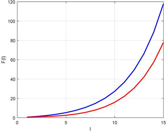
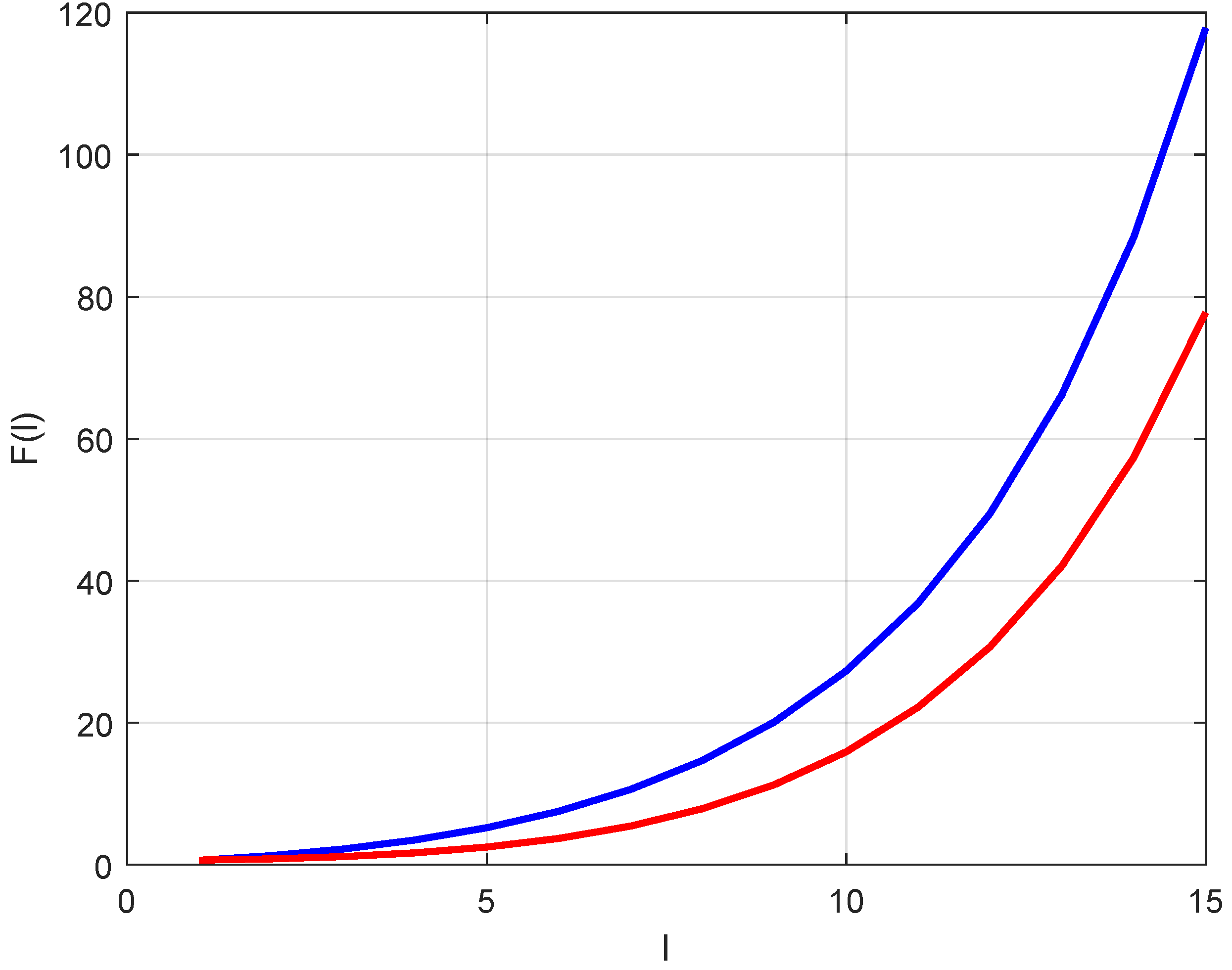
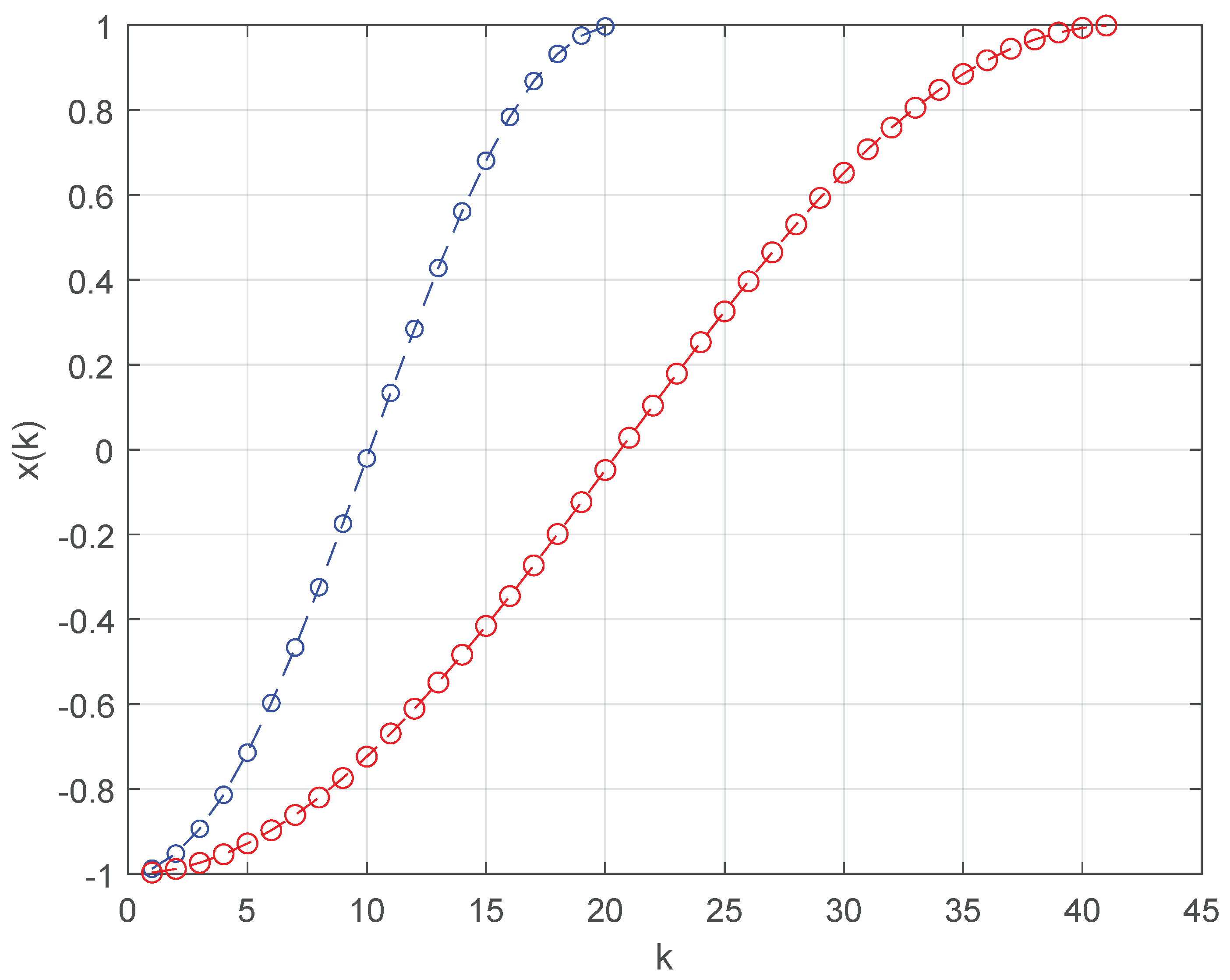
The exact value of the integral $I\left(f\right)$ is about $7.898964$. In this example, the rules $Q_{2\mathcal{\ell }+1}^L,Q_{2\mathcal{\ell }+1}^S$, and $Q_{2\mathcal{\ell }+1}^{1/4}$ have a node smaller than $-1$. They therefore cannot be used for error estimation. Table 9 in [26] shows the error estimates $E_W$ and $E_T$ for some values of ℓ. We show these estimates in Table 2 as well as error estimates $E_{NAG}$. Since $\gamma =1.01$ and $\delta =1.0001$, it follows from Theorem 1 that the quadrature rule ${\widehat{Q}}_{2\mathcal{\ell }+1}$ is internal for a sufficiently large ℓ. Numerical computations confirm that the rules are internal for $\mathcal{\ell }\ge 5$. Figure 1 displays the left-hand sides of inequalities (18) and (20) for the case where $\gamma =1.01$ and $\delta =1.0001$ as functions of ℓ, which we denote by $F(\mathcal{\ell })$, in the interval $[1,15]$. The blue curve depicts the function on the left-hand side of inequality (18), and the red curve shows the function on the left-hand side of inequality (20). In this example, the NAG quadrature rules ${\widehat{Q}}_{2\mathcal{\ell }+1}$ are internal for all $\mathcal{\ell }\ge 1$.

Table 2. Error estimates and the magnitude of the true error for Example 2.

ℓ	${\mathit{E}}_{\mathit{N}\mathit{A}\mathit{G}}\left(\mathit{f}\right)$	${\mathit{E}}_{\mathit{W}}\left(\mathit{f}\right)$	${\mathit{E}}_{\mathit{T}}\left(\mathit{f}\right)$	Error
5	$4.9504(-8)$	$4.4724(-8)$	$4.4505(-8)$	$4.9283(-8)$
10	$4.1303(-10)$	$3.7565(-10)$	$2.8957(-10)$	$4.1252(-10)$
15	$2.8451(-11)$	$2.6923(-11)$	$1.5803(-11)$	$2.8610(-11)$
20	$4.5227(-12)$	$4.3944(-12)$	$2.0560(-12)$	$4.5686(-12)$
30	$3.6413(-13)$	$3.6189(-13)$	$1.2036(-13)$	$3.6908(-13)$

Figure 1. The graphs $F(\mathcal{\ell })$ of the left-hand sides of inequalities (18) [blue graph] and (20) [red graph]. The graphs represent the conditions of internality of the quadrature rule ${\widehat{Q}}_{2\mathcal{\ell }+1}$ at the left and the right endpoints of the interval $[-1,1]$, respectively.

We note that the error estimates $E_{NAG}\left(f\right)$ are more accurate than the error estimates $E_W\left(f\right)$ and $E_T\left(f\right)$.

Example 3.

This example is an extension of [26] [Example 6.4]. Let

$$f\left(x\right)={(1-x)}^{3}ln(1-x)\mathrm{and}d\widehat{\sigma }\left(x\right)={\displaystyle \frac{x-5}{x-1.25}}\sqrt{{\displaystyle \frac{1+x}{1-x}}}dx.$$

The true value of the integral is $I\left(f\right)\approx 1.454037$. The rules $Q_{2\mathcal{\ell }+1}^L$, $Q_{2\mathcal{\ell }+1}^S$, and $Q_{2\mathcal{\ell }+1}^{1/4}$ cannot be evaluated. Table 11 in [26] shows the error estimates $E_W$ and $E_T$ for some ℓ-values. We also show these values in Table 3 to allow easy comparison with the error estimates $E_{NAG}$. As $\gamma =-5$ and $\delta =-1.25$, it follows from Theorem 2 that the quadrature rule ${\widehat{Q}}_{2\mathcal{\ell }+1}$ is internal for a sufficiently large ℓ. Numerical computations confirm that the rules are internal for $\mathcal{\ell }\ge 5$. The nodes and coefficients of the quadrature rule ${\widehat{Q}}_{2\mathcal{\ell }+1}$ for $\mathcal{\ell }=10$ are reported in Table 4. The error estimate $E_{NAG}\left(f\right)$ can be seen to be of about the same quality as the error estimate $E_W\left(f\right)$ and is more accurate than the estimate $E_T\left(f\right)$.

Table 3. Error estimates and the magnitude of the true error for Example 3.

ℓ	${\mathit{E}}_{\mathit{N}\mathit{A}\mathit{G}}\left(\mathit{f}\right)$	${\mathit{E}}_{\mathit{W}}\left(\mathit{f}\right)$	${\mathit{E}}_{\mathit{T}}\left(\mathit{f}\right)$	Error
5	$6.0739(-4)$	$6.1393(-4)$	$5.4118(-4)$	$6.1114(-4)$
10	$6.9228(-6)$	$7.0224(-6)$	$4.8492(-6)$	$6.9755(-6)$
15	$4.8769(-7)$	$4.9514(-7)$	$2.7652(-7)$	$4.9155(-7)$
20	$7.2500(-8)$	$7.3633(-8)$	$3.4382(-8)$	$7.3081(-8)$
30	$4.7831(-9)$	$4.8590(-9)$	$1.7034(-9)$	$4.8216(-9)$

Table 4. The nodes and coefficients of the two-measure-based generalized Gauss quadrature rule, i.e., the NAG quadrature rule, ${\widehat{Q}}_{2\mathcal{\ell }+1}$ ($\mathcal{\ell }=10$) with respect to the measures $d{\widehat{\sigma }}_3\left(x\right)$, in the case where $\gamma =-5,\delta =-1.25$, and $d\mu \left(x\right)=\sqrt{1-x^2}dx$.

k	The Nodes ${\mathit{x}}_{\mathit{k}}$	The Coefficients ${\mathit{\sigma }}_{\mathit{k}}$
1	$-0.98910025340381332329$	$0.00430845907332257640$
2	$-0.95663891941087701172$	$0.01729747954854571653$
3	$-0.90332468406842124467$	$0.03916565485043396239$
4	$-0.83032201859170628069$	$0.07027023386275711194$
5	$-0.73922651381457788629$	$0.11116909921494881111$
6	$-0.63203102111081864757$	$0.16268503479968968656$
7	$-0.51108324221869106853$	$0.22599852907677552106$
8	$-0.37903554963582356450$	$0.30277817032094049856$
9	$-0.23878792305698338706$	$0.39536102232723992938$
10	$-0.09342494473514211522$	$0.50699856053924623883$
11	$0.05385220626525179885$	$0.64218443547912713654$
12	$0.19979790256502880290$	$0.80707172294576802838$
13	$0.34119768498453416558$	$1.00995172508579420322$
14	$0.47494697906631608153$	$1.26166108040035500436$
15	$0.59813295343076826732$	$1.57551496136577015947$
16	$0.70811987017732732004$	$1.96576049177444377322$
17	$0.80263767267093890566$	$2.44243435228485352437$
18	$0.87986969897975410751$	$2.99930301210226900850$
19	$0.93852366343451706677$	$3.59311451254722265071$
20	$0.97784768454641332819$	$4.12373102638658114159$
21	$0.99753849670918278329$	$4.44677799217834906935$

The nodes $x_k(k=1,2,\cdots ,2\mathcal{\ell }+1)$ of the two-measure-based generalized Gauss quadrature rule, i.e., the NAG quadrature rule,

$${\widehat{Q}}_{2\mathcal{\ell }+1}=\sum _{k=1}^{2\mathcal{\ell }+1}{\sigma }_{k}f\left(x_k\right),$$

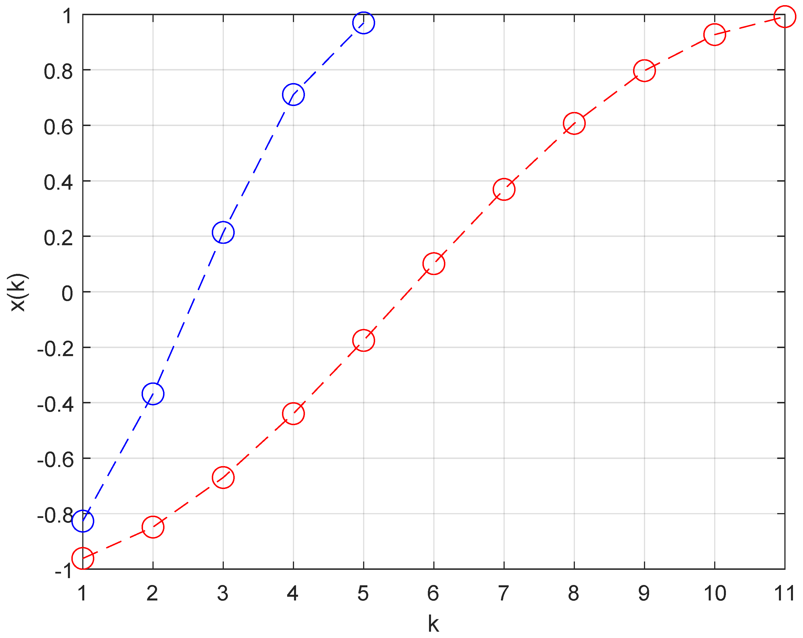
with respect to the measure $d{\widehat{\sigma }}_3\left(x\right)$, in the case $\gamma =-5,\delta =-1.25$, and $d\mu \left(x\right)=\sqrt{1-x^2}dx$, depend on k. Namely, $x_k=x\left(k\right)(k=1,2,\cdots ,2\mathcal{\ell }+1)$. Their distribution compared to the corresponding Gaussian rule $G_{\mathcal{\ell }}$ nodes is displayed in Figure 2 for $\mathcal{\ell }=5$ and in Figure 3 for $\mathcal{\ell }=20$. We performed many more numerical tests that confirmed the same behavior of the nodes $x_k$, and observed that $x_{2k}\approx x_k^G(k=1,2,\cdots ,\mathcal{\ell })$. This means that the two-measure-based generalized Gauss quadrature rule, i.e., the NAG quadrature rule, ${\widehat{Q}}_{2\mathcal{\ell }+1}={\sum }_{k=1}^{2\mathcal{\ell }+1}{\sigma }_{k}f\left(x_k\right)$ has a similar structure as the averaged $Q_{2\mathcal{\ell }+1}^L$, generalized averaged $Q_{2\mathcal{\ell }+1}^S$, and weighted averaged $Q_{2\mathcal{\ell }+1}^{1/4}$, $Q_{2\mathcal{\ell }+1}^W$ Gaussian quadrature rules, and that only the outermost nodes of ${\widehat{Q}}_{2\mathcal{\ell }+1}$, i.e., $x_1,x_{2\mathcal{\ell }+1}$, may be outside of the interval $[-1,1]$. It could be of interest to prove this hypothesis. Of course, in this specific case, both of the outermost nodes are internal.

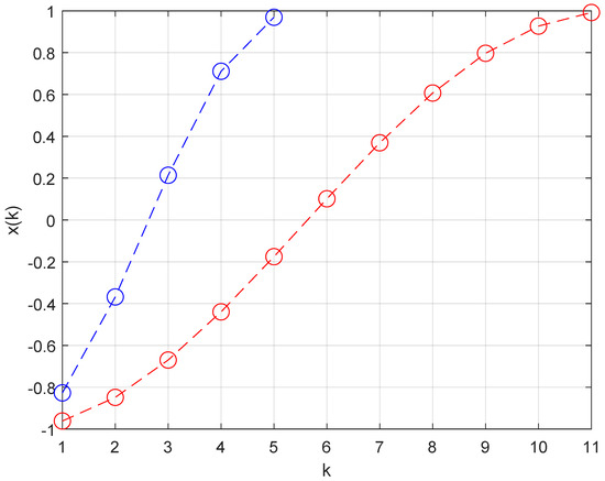
Figure 2. The distribution nodes $x\left(k\right)=x_k$ of the NAG quadrature rule ${\widehat{Q}}_{2\mathcal{\ell }+1}$ (marked by red circels) compared to the corresponding Gaussian rule $G_{\mathcal{\ell }}$ nodes (marked by blue circels), for $\mathcal{\ell }=5$.

Figure 3. The distribution nodes $x\left(k\right)=x_k$ of the NAG quadrature rule ${\widehat{Q}}_{2\mathcal{\ell }+1}$ (marked by red circels) compared to the corresponding Gaussian rule $G_{\mathcal{\ell }}$ nodes (marked by blue circels), for $\mathcal{\ell }=20$.

Example 4.

This example is associated with Example 3, only the integrand is different. Let

$$f\left(x\right)={\left(1-\left|x\right|\right)}^{3}ln(1-x)\mathrm{and}d\widehat{\sigma }\left(x\right)={\displaystyle \frac{x-5}{x-1.25}}\sqrt{{\displaystyle \frac{1+x}{1-x}}}dx.$$

The true value of the integral is $I\left(f\right)\approx -0.446367$. The rules $Q_{2\mathcal{\ell }+1}^L$, $Q_{2\mathcal{\ell }+1}^S$, and $Q_{2\mathcal{\ell }+1}^{1/4}$ cannot be evaluated. Table 5 shows the error estimates $E_{NAG},E_W,E_T$ for some ℓ-values and the actual errors. Numerical computations for this integrand confirm that the error estimate $E_{NAG}\left(f\right)$ can be seen to be of about the same quality as the error estimate $E_W\left(f\right)$. In this case, the error estimates $E_{NAG}\left(f\right)$ are a little bit closer to the actual error than the error estimates $E_W\left(f\right)$.

Table 5. Error estimates and the magnitude of the true error for Example 4.

ℓ	${\mathit{E}}_{\mathit{N}\mathit{A}\mathit{G}}\left(\mathit{f}\right)$	${\mathit{E}}_{\mathit{W}}\left(\mathit{f}\right)$	${\mathit{E}}_{\mathit{T}}\left(\mathit{f}\right)$	Error
10	$1.2074(-2)$	$9.9378(-3)$	$4.7027(-3)$	$1.1168(-2)$
20	$1.5002(-3)$	$1.2173(-3)$	$3.4647(-4)$	$1.3824(-3)$
30	$4.4036(-4)$	$3.5508(-4)$	$7.1868(-5)$	$4.0510(-4)$
40	$1.8462(-4)$	$1.4835(-4)$	$2.3267(-5)$	$1.6969(-4)$
50	$9.4124(-5)$	$7.5462(-5)$	$9.6568(-6)$	$8.6469(-5)$

6. Conclusions

Our interest in modifications of Chebyshev weight functions stems from the attention that modification methods and their applications, e.g., to computing the Hilbert transform, have received in the literature; see Gautschi [3] [Section 2.4] for a thorough discussion of modification algorithms and some applications. This paper analyzes the application of NAG quadrature rules to the estimation of the quadrature error $|I\left(f\right)-G_{\mathcal{\ell }}\left(f\right)|$, where $I\left(f\right)$ is an integral with a modified Chebyshev measure and $G_{\mathcal{\ell }}$ is the ℓ-node Gauss quadrature rule. Our analysis shows that interior NAG rules can be constructed when averaged or generalized averaged quadrature rules are not interior. The NAG rules therefore can be applied to a larger class of integrands than the averaged and generalized averaged rules. In this paper, these cases are covered by Theorems 1 and 2. For future work, it would be of interest to consider the internality of two-measure-based quadrature rules, i.e., of NAG quadrature rules, for some other measures and their modifications when the auxiliary measure $d\mu$ is different from the Chebyshev measure of the second kind.

References

- Gautschi, W. Orthogonal polynomials and quadrature. Electron. Trans Numer. Anal. 1999, 9, 65–76. [Google Scholar]
- Gautschi, W. The interplay between classical analysis and (numerical) linear algebra—A tribute to Gene H. Golub. Electron. Trans. Numer. Anal. 2002, 13, 119–147. [Google Scholar]
- Gautschi, W. Orthogonal Polynomials: Computation and Approximation; Oxford University Press: Oxford, UK, 2004. [Google Scholar]
- Gautschi, W. Orthogonal Polynomials in MATLAB: Exercises and Solutions; SIAM: Philadelphia, PA, USA, 2016. [Google Scholar]
- Gautschi, W.; Milovanović, G.V. Binet-type polynomials and their zeros. Eletron. Trans. Numer. Anal. 2018, 50, 52–70. [Google Scholar] [CrossRef]
- Pejčev, A.V.; Reichel, L.; Spalević, M.M.; Spalević, M.S. A new class of quadrature rules for estimating the error in Gauss quadrature. Appl. Numer. Math. 2024, 204, 206–221. [Google Scholar] [CrossRef]
- Djukić, D.L.; Mutavdžić Djukić, R.M.; Pejčev, A.V.; Reichel, L.; Spalević, M.M.; Spalević, S.M. Internality of two-measure-based generalized Gauss quadrature rules for modified Chebyshev measures. Electron. Trans. Numer. Anal. 2024, 61, 157–172. [Google Scholar] [CrossRef]
- Gautschi, W. A historical note on Gauss–Kronrod quadrature. Numer. Math. 2005, 100, 483–484. [Google Scholar] [CrossRef]
- Kahaner, D.K.; Monegato, G. Nonexistence of extended Gauss-Laguerre and Gauss-Hermite quadrature rules with positive weights. Z. Angew. Math. Phys. 1978, 29, 983–986. [Google Scholar] [CrossRef]
- Monegato, G. Stieltjes polynomials and related quadrature rules. SIAM Rev. 1982, 24, 137–158. [Google Scholar] [CrossRef]
- Peherstorfer, F.; Petras, K. Ultraspherical Gauss–Kronrod quadrature is not possible for λ > 3. SIAM J. Numer. Anal. 2000, 37, 927–948. [Google Scholar] [CrossRef]
- Peherstorfer, F.; Petras, K. Stieltjes polynomials and Gauss–Kronrod quadrature for Jacobi weight functions. Numer. Math. 2003, 95, 689–706. [Google Scholar] [CrossRef]
- Notaris, S. Gauss–Kronrod quadrature formulae—A survey of fifty years of research. Electron. Trans. Numer. Anal. 2016, 45, 371–404. [Google Scholar]
- Calvetti, D.; Golub, G.H.; Gragg, W.B.; Reichel, L. Computation of Gauss–Kronrod rules. Math. Comp. 2000, 69, 1035–1052. [Google Scholar] [CrossRef]
- Laurie, D.P. Calculation of Gauss–Kronrod quadrature rules. Math. Comp. 1997, 66, 1133–1145. [Google Scholar] [CrossRef]
- Laurie, D.P. Anti-Gaussian quadrature formulas. Math. Comp. 1996, 65, 739–747. [Google Scholar] [CrossRef]
- Spalević, M.M. On generalized averaged Gaussian formulas. Math. Comp. 2007, 76, 1483–1492. [Google Scholar] [CrossRef]
- Peherstorfer, F. On positive quadrature formula. In Numerical Integration IV; Brass, H., Hämmerlin, G., Eds.; ISNM International Series of Numerical Mathematics; Birkhäuser: Basel, Switzerland, 1993; Volume 112, pp. 297–313. [Google Scholar]
- Peherstorfer, F. Positive quadrature formulas III: Asymptotics of weights. Math. Comp. 2008, 77, 2241–2259. [Google Scholar] [CrossRef]
- Alqahtani, H.; Borges, C.F.; Djukić, D.L.; Mutavdžić Djukić, R.M.; Reichel, L.; Spalević, M.M. Computation of pairs of related quadrature rules. Appl. Numer. Math. 2025, 208, Pt A, 32–42. [Google Scholar] [CrossRef]
- Borges, C.F.; Reichel, L. Computation of Gauss-type quadrature rules. Electron. Trans. Numer. Anal. 2024, 61, 121–136. [Google Scholar] [CrossRef]
- Reichel, L.; Spalević, M.M. Generalized averaged Gaussian quadrature formulas: Properties and applications. J. Comput. Appl. Math. 2022, 410, 114232. [Google Scholar] [CrossRef]
- Djukić, D.L.; Mutavdzić Djukić, R.M.; Reichel, L.; Spalević, M.M. Internality of generalized averaged Gauss quadrature rules and truncated variants for modified Chebyshev measures of the first kind. J. Comput. Appl. Math. 2021, 398, 113696. [Google Scholar] [CrossRef]
- Djukić, D.L.; Mutavdzić Djukić, R.M.; Reichel, L.; Spalević, M.M. Internality of generalized averaged Gauss quadrature rules and truncated variants for modified Chebyshev measures of the third and fourth kinds. Numer. Algorithms 2023, 92, 523–544. [Google Scholar] [CrossRef]
- Djukić, D.L.; Reichel, L.; Spalević, M.M.; Tomanović, J.D. Internality of generalized averaged Gaussian quadrature rules and truncated variants for modified Chebyshev measures of the second kind. J. Comput. Appl. Math. 2019, 345, 70–85. [Google Scholar] [CrossRef]
- Djukić, D.L.; Mutavdzić Djukić, R.M.; Reichel, L.; Spalević, M.M. Weighted averaged Gaussian quadrature rules for modified Chebyshev measures. Appl. Numer. Math. 2024, 200, 195–208. [Google Scholar] [CrossRef]
- Golub, G.H.; Welsch, J.H. Calculation of Gauss quadrature rules. Math. Comp. 1969, 23, 221–230. [Google Scholar] [CrossRef]
- Djukić, D.L.; Reichel, L.; Spalević, M.M. Truncated generalized averaged Gauss quadrature rules. J. Comput. Appl. Math. 2016, 308, 408–418. [Google Scholar] [CrossRef]
Disclaimer/Publisher’s Note: The statements, opinions and data contained in all publications are solely those of the individual author(s) and contributor(s) and not of MDPI and/or the editor(s). MDPI and/or the editor(s) disclaim responsibility for any injury to people or property resulting from any ideas, methods, instructions or products referred to in the content. |
© 2025 by the authors. Licensee MDPI, Basel, Switzerland. This article is an open access article distributed under the terms and conditions of the Creative Commons Attribution (CC BY) license (https://creativecommons.org/licenses/by/4.0/).