Estimation for Partial Functional Multiplicative Regression Model

Abstract

Functional data such as curves, shapes, and manifolds have become more and more common with modern technological advancements. The multiplicative regression model is well suited for analyzing data with positive responses. In this study, we study the estimation problems of the partial functional multiplicative regression model (PFMRM) based on the least absolute relative error (LARE) criterion and least product relative error (LPRE) criterion. The functional predictor and slope function are approximated by the functional principal component basis functions. Under certain regularity conditions, we derive the convergence rate of the slope function and establish the asymptotic normality of the slope vector for two estimation methods. Monte Carlo simulations are carried out to evaluate the proposed methods, and an application to Tecator data is investigated for illustration.

1. Introduction

We consider the PFMRM which includes some scalar covariates and a functional predictor, paired with a scalar response. That is,

$$Y=\exp \left({\mathit{Z}}^{\top }\mathit{\alpha }+{\int }_T\beta \left(t\right)X\left(t\right)dt\right)ϵ,$$

(1)

where Y is a positive response variable; $\mathit{Z}={(Z_1,\dots ,Z_p)}^{\top }$ is a p-dimensional vector covariate, $\mathit{\alpha }={({\alpha }_1,\dots ,{\alpha }_p)}^{\top }$ is the p-vector of slope coefficients, in which p is assumed to be fixed; $\beta \left(t\right)\in L^2\left(T\right)$ is the unknown slope function associated with functional predictor $X\left(t\right)$; and $ϵ$ is a positive random error independent of $\mathit{Z}$ and $X\left(t\right)$. Here, the Hilbert space $L^2\left(T\right)$ is the set of all square integrable functions on T, endowed with the inner product $⟨x,Y⟩={\int }_{T}x\left(t\right)Y\left(t\right)dt$ and the norm $\parallel x\parallel ={⟨x,x⟩}^{1/2}$. The model (1) generalizes both the classic multiplicative regression model [1] and the functional multiplicative regression model [2] that correspond to the cases of $\beta \left(t\right)=0$ and $\mathit{\alpha }=0$, respectively. When the log transformation applies to this model, the above model simply degrades to a partial functional linear regression model [3]. When the response variable Y is a failure time, model (1) is called the functional accelerated failure time model in survival analysis; see [4] for example. For simplicity of notation, we assume that $T=[0,1]$, and $\mathit{Z}$ and $X\left(t\right)$ have zero mean throughout the study.

In many applications, the response variable is positive, for example, survival time, stock prices, income, body fat level, emissions of nitrogen oxides, and the value of owner-occupied homes frequently arise in statistical practice. The multiplicative regression model plays an important role in describing these types of data. To estimate the multiplicative regression models, Refs. [1,5] proposed LARE and LPRE estimation, respectively. The LARE criterion minimizes ${\sum }_{i=1}^n\left(\left|{ϵ}_i^{-1}-1\right|+\left|{ϵ}_i-1\right|\right)$, and the LPRE criterion minimizes ${\sum }_{i=1}^n\left(\left|{ϵ}_i^{-1}-1\right|\times \left|{ϵ}_i-1\right|\right)$, which is equivalent to minimizing ${\sum }_{i=1}^n\left({ϵ}_i^{-1}+{ϵ}_i\right)$. As pointed out by [5], the LARE estimation is robust and scale-free, but optimization of its use may be challenging as the objective function minimized is non-smoothing. In addition, confidence intervals for parameters are not very accurate due to the complexity of the asymptotic covariance matrix, which involves the density of the model error. In order to overcome the shortcoming of LARE, Ref. [5] proposed the LPRE criterion, which is strictly convex and infinitely differentiable, and the optimization procedure is much easier. In recent years, due to the excellent properties of LARE and LPRE estimation, scholars in various fields have been attracted to conducting extended research on them. The readers can refer to [6,7,8].

For functional multiplicative models, to the best of our knowledge, there are only a few works and all of them focus on the above two criteria. For example, Ref. [9] developed the functional quadratic multiplicative model and derived the asymptotic properties of the estimator with the LARE criterion. Later, Refs. [2,10] considered the variable selection for partially and locally sparse functional linear multiplicative models based on the LARE criterion. In this paper, we consider the modeling of a positive scalar response variable with both scalar and functional predictors under the PFMRM. The above two criteria are employed to estimate the parametric vector $\mathit{\alpha }$ and the slope function $\beta \left(t\right)$ in model (1).

The major contributions of this paper are four-fold. First, this study first extends the LPRE criterion to the estimation of functional regression models. Second, we estimate the unknown slope function and functional predictor by using a functional principal component analysis technique, derive the convergence rates of the slope function, and establish the asymptotic normality of the parameter vector under mild regularity conditions for two estimation methods. Third, we develop an iterative algorithm to solve the involved optimization problem and propose a data-driven procedure to select the tuning parameters. Finally, we conduct extensive numerical studies to examine the finite sample performance of the proposed methods and find that the LPRE method has better performance than the LARE, least square, and least absolute deviation methods.

The rest of the article is organized as follows. Section 2 describes the detailed estimation procedures for model (1). Section 3 is dedicated to the asymptotic study of our estimators. The feasible algorithm for estimations of the parameters and nonparametric functions of PFMRM is proposed based on the LPRE criterion and presented in Section 4. Section 5 conducts simulation studies to evaluate the finite sample performance of the proposed methods. In Section 6, we apply the proposed method to the Tecator data. The article concludes with a discussion in Section 7. Proofs are provided in Appendix A.

2. Estimation Method

Let $\left({\mathit{Z}}_i,X_i(·),Y_i,{ϵ}_i\right)$, $i\in \{1,\dots ,n\}$ be the independent realizations of $\left(\mathit{Z},X(·),Y,ϵ\right)$ generated from model (1), that is,

$$Y_i=\exp \left({\mathit{Z}}_i^{\top }\mathit{\theta }+{\int }_0^1\beta \left(t\right)X_i\left(t\right)dt\right){ϵ}_i,i\in \{1,\dots ,n\},$$

(2)

where random errors ${ϵ}_i$, $i\in \{1,\dots ,n\}$ are independent and identically distributed (i.i.d.) and independent of ${\mathit{Z}}_i$ and $X_i(·)$.

The covariance and empirical covariance functions of $X(·)$ can be defined as

$$C_X(t,s)=\mathrm{Cov}(X\left(t\right),X\left(s\right)),{\widehat{C}}_X(t,s)={\displaystyle \frac{1}{n}}\sum _{i=1}^n{X}_i\left(t\right)X_i\left(s\right).$$

According to Mercer’s theorem, the spectral expansions of $C_X$ and ${\widehat{C}}_X$ can be written as

$$C_X(t,s)=\sum _{j=1}^{\infty }{\lambda }_j{v}_j\left(t\right)v_j\left(s\right),{\widehat{C}}_X(t,s)=\sum _{j=1}^{\infty }{\widehat{\lambda }}_j{\widehat{v}}_j\left(t\right){\widehat{v}}_j\left(s\right),$$

where ${\lambda }_1>{\lambda }_2>\cdots >0$ and ${\widehat{\lambda }}_1\ge {\widehat{\lambda }}_2\ge \cdots \ge {\widehat{\lambda }}_{n+1}=\cdots =0$ are the ordered eigenvalue sequences of the linear operators with kernels $C_X$ and ${\widehat{C}}_X$, respectively, and ${\left\{v_j(·)\right\}}_{j=1}^{\infty }$ and ${\left\{{\widehat{v}}_j(·)\right\}}_{j=1}^{\infty }$ are appropriate orthonormal eigenfunction sequences. With a slight abuse of notation, we use $C_X$ to denote both the covariance operator and the covariance function of $X(·)$. We assume that the covariance operator $C_X$ defined by $C_{X}f\left(s\right)={\int }_0^1{C}_X(t,s)f\left(t\right)dt$ is strictly positive. In addition, $\left\{{\widehat{v}}_j(·),{\widehat{\lambda }}_j\right\}$ can be regarded as an estimator of $\left\{v_j(·),{\lambda }_j\right\}$.

On the basis of the Karhunen–Loève decomposition, $\beta \left(t\right)$ and $X_i\left(t\right)$ can be expanded to

$$\beta \left(t\right)=\sum _{j=1}^{\infty }{\gamma }_j{v}_j\left(t\right),X_i\left(t\right)=\sum _{j=1}^{\infty }{\xi }_{ij}{v}_j\left(t\right),i\in \{1,\dots ,n\},$$

(3)

where ${\gamma }_j=⟨\beta (·),v_j(·)⟩={\int }_0^1\beta \left(t\right)v_j\left(t\right)dt$, and ${\xi }_{ij}=⟨X_i(·),v_j(·)⟩$ represents the coordinate of the ith curve with respect to the jth eigenbasis.

Analogously, we define $C_{YX}(·)=\mathrm{Cov}(Y,X(·))$, $C_{\mathit{Z}}=\mathrm{Var}\left(\mathit{Z}\right)$, $C_{\mathit{Z}Y}=\mathrm{Cov}(\mathit{Z},Y)$, and $C_{\mathit{Z}X}(·)=\mathrm{Cov}(\mathit{Z},X(·))={(C_{Z_{1}X}(·),\dots ,C_{Z_{p}X}(·))}^{\top }$. Then, their corresponding empirical counterparts can be defined as

$${\widehat{C}}_{YX}={\displaystyle \frac{1}{n}}\sum _{i=1}^n{Y}_i{X}_i,{\widehat{C}}_{\mathit{Z}}={\displaystyle \frac{1}{n}}\sum _{i=1}^n{\mathit{Z}}_i{\mathit{Z}}_{\mathit{i}}^{\top },{\widehat{C}}_{\mathit{Z}Y}={\displaystyle \frac{1}{n}}\sum _{i=1}^n{\mathit{Z}}_i{Y}_i,{\widehat{C}}_{\mathit{Z}X}={\displaystyle \frac{1}{n}}\sum _{i=1}^n{\mathit{Z}}_i{X}_i.$$

Given the orthogonality of $\{v_1(·),\dots ,v_m(·)\}$ and (3), model (2) can be rewritten as

$$Y_i=\exp \left({\mathit{Z}}_i^{\top }\mathit{\alpha }+\sum _{j=1}^m{\gamma }_j{\xi }_{ij}\right){\widetilde{ϵ}}_i=\exp ({\mathit{Z}}_i^{\top }\mathit{\alpha }+{\mathit{U}}_i^{\top }\mathit{\gamma }){\widetilde{ϵ}}_i,(i=1,\dots ,n)$$

where ${\mathit{U}}_i={({\xi }_{i1},\dots ,{\xi }_{im})}^{\top }$, $\mathit{\gamma }={({\gamma }_1,\dots ,{\gamma }_m)}^{\top }$, ${\widetilde{ϵ}}_i=\exp \left({\sum }_{j=m+1}^{\infty }{\gamma }_j{\xi }_{ij}\right){ϵ}_i$, and the truncation parameter $m\to \infty$ as $n\to \infty$.

2.1. LARE Estimation

This is based on the LARE criterion of [1] and ${\upsilon }_j(·)$ is replaced with its estimator ${\widehat{\upsilon }}_j(·)$. The LARE estimates of model (1) can be obtained by minimizing the following loss functions:

$$(\widehat{\mathit{\alpha }},\widehat{\mathit{\gamma }})\triangleq \arg \underset{(\mathit{\alpha },\mathit{\gamma })}{\min }\sum _{i=1}^n\left\{\left|{\displaystyle \frac{Y_i-\exp ({\mathit{Z}}_i^{\top }\mathit{\alpha }+{\widehat{\mathit{U}}}_i^{\top }\mathit{\gamma })}{Y_i}}\right|+\left|{\displaystyle \frac{Y_i-\exp ({\mathit{Z}}_i^{\top }\mathit{\alpha }+{\widehat{\mathit{U}}}_i^{\top }\mathit{\gamma })}{\exp ({\mathit{Z}}_i^{\top }\mathit{\alpha }+{\widehat{\mathit{U}}}_i^{\top }\mathit{\gamma })}}\right|\right\},$$

(4)

where ${\widehat{\mathit{U}}}_i={({\widehat{\xi }}_{i1},\cdots ,{\widehat{\xi }}_{im})}^{\top }$ with ${\widehat{\xi }}_{ij}=⟨X_i(·),{\widehat{\upsilon }}_j(·)⟩$, $\widehat{\mathit{\gamma }}={({\widehat{\gamma }}_1,\dots ,{\widehat{\gamma }}_m)}^{\top }$. Moreover, we can obtain the LARE estimator $\widehat{\beta }\left(t\right)={\sum }_{j=1}^m{\widehat{\gamma }}_j{\widehat{\upsilon }}_j\left(t\right)$.

2.2. LPRE Estimation

This is based on the LPRE criterion of [5] and ${\upsilon }_j(·)$ is replaced with its estimator ${\widehat{\upsilon }}_j(·)$. The LPRE estimates of model (1) can be obtained by minimizing the following loss functions:

$$(\tilde{\mathit{\alpha }},\tilde{\mathit{\gamma }})\triangleq \arg \underset{(\mathit{\alpha },\mathit{\gamma })}{\min }\sum _{i=1}^n\left\{Y_i\exp (-{\mathit{Z}}_i^{\top }\mathit{\alpha }-{\widehat{\mathit{U}}}_i^{\top }\mathit{\gamma })+Y_i^{-1}\exp ({\mathit{Z}}_i^{\top }\mathit{\alpha }+{\widehat{\mathit{U}}}_i^{\top }\mathit{\gamma })-2\right\},$$

(5)

where $\tilde{\mathit{\gamma }}={({\tilde{\gamma }}_1,\dots ,{\tilde{\gamma }}_m)}^{\top }$. Moreover, we can obtain the LPRE estimator $\tilde{\beta }\left(t\right)={\sum }_{j=1}^m{\tilde{\gamma }}_j{\widehat{\upsilon }}_j\left(t\right)$.

3. Asymptotic Properties

In this section, we establish the asymptotic properties of the estimators. Formulating the results requires the following technical assumptions. Firstly, we present some notations. Suppose that ${\mathit{\alpha }}_0$ and ${\beta }_0\left(t\right)$ are the true values of $\mathit{\alpha }$ and $\beta \left(t\right)$, respectively, and let ${\mathit{\gamma }}_0={({\gamma }_{01},\dots ,{\gamma }_{0m})}^{\top }$ be the true score coefficient vector. The notation $\parallel ·\parallel$ denotes the norm ${\mathcal{L}}^2$ for a function or the Euclidean norm for a vector. In what follows, c denotes a generic positive constant that may take various values. Moreover, $a_n\sim b_n$ implies that $a_n/b_n$ is bounded away from zero and infinity as $n\to \infty$.

C1.

The random process $X(·)$ and the score ${\xi }_i$ satisfy the following conditions:

$${E\left|\right|X(·)\left|\right|}^4\le \infty ,E{\left({\xi }_i\right)}^4\le c{\lambda }_i^2, i\ge 1.$$

C2.

For the eigenvalues of the linear operator $C_X$ and the score coefficients, the following conditions hold:

$\left(\mathit{a}\right)$ There exist some constants c and $a>1$ such that $c^{-1}{i}^{-a}\le {\lambda }_i\le c{i}^{-a}, {\lambda }_i-{\lambda }_{i+1}\ge c{i}^{-a-1},i\ge 1$;

$\left(\mathit{b}\right)$ There exist some constants c and $b>a/2+1$ such that $|{\gamma }_j| \le c{j}^{-b},j\ge 1$.

C3.

The tuning parameter $m\sim n^{1/(a+2b)}$.

C4.

For the random vector $\mathit{Z}$, ${E\parallel \mathit{Z}\parallel }^4<\infty .$

C5.

There exists some constant c such that $\mid ⟨C_{Z_{l}X},v_j⟩\mid \le c{j}^{-(a+b)},l=1,\cdots , p,j\ge 1$.

C6.

Let ${\eta }_{ik}=Z_{ik}-⟨g_k,X_i⟩$ with $g_k={\displaystyle \sum _{j=1}^{\infty }}{\lambda }_j^{-1}⟨C_{Z_{k}X},v_j⟩v_j$, for each k, then ${\eta }_{1k},\cdots ,{\eta }_{nk}$ are independent and identically distributed random variables. Assume that

$$E\left[{\eta }_{1k}\right|X_1,\cdots ,X_n]=0,E\left[{\eta }_{1k}^2\right|X_1,\cdots ,X_n]={\mathrm{\Sigma }}_{kk},$$

where ${\mathrm{\Sigma }}_{kk}$ is the kth diagonal element of $\mathrm{\Sigma }=E\left({\mathit{\eta }}_i{{\mathit{\eta }}_i}^{\top }\right)$ with ${\mathit{\eta }}_i={({\eta }_{i1},\cdots ,{\eta }_{ip})}^{\top }$, and $\mathrm{\Sigma }$ is a positive definite matrix.

C7.

The error $ϵ$ has a continuous density $f(·)$ in a neighborhood of 1, and is independent of $(\mathit{Z},X(·\left)\right)$.

C8.

$\mathrm{P}(ϵ>0)=1$, $E(ϵ+{ϵ}^{-1})<\infty$, $E\left[(ϵ+{ϵ}^{-1})\mathrm{sgn}(ϵ-1)\right]=0$ and $E\left[{({ϵ}^{-1}+ϵ)}^2\right]<\infty$.

C9.

$E\left[(ϵ-{ϵ}^{-1})\right]=0$, $E\left[{({ϵ}^{-1}+ϵ)}^2\right]<\infty$.

Remark 1. 

C1–C3 are standard assumptions used in classical functional linear regression (see, e.g., [11,12]). More specifically, C1 is needed for the consistency of ${\widehat{C}}_X(t,s)$. C2(a) is required to identify the slope function $\beta \left(t\right)$ by preventing the spacing between the eigenvalues from being too small, while C2 (b) is used to make the slope function $\beta \left(t\right)$ sufficiently smooth. C3 is required to obtain the convergence rate of the slope function $\beta \left(t\right)$. C4–C6 are used to handle the linear part of the vector-type covariate in the model, which are similar to [3,13]. C4 is a little stronger than those in classical linear models and is primarily used to ensure the asymptotic behavior of ${\widehat{C}}_{\mathit{Z}X}$ and ${\widehat{C}}_{\mathit{Z}}$. C5 makes the effect of truncation on the estimation of $\beta (·)$ small enough. Notably, ${\mathit{\eta }}_{ik}$ is the regression error of $Z_{ik}$ on $X_i(·)$, and the conditions on ${\mathit{\eta }}_s$ in C6 essentially restrict that $\mathit{Z}$ can only be linearly related to $X(·)$. C6 is also used to establish the asymptotic normality of the parameter estimator, in a similar manner to that applied in [3,13] for modeling the dependence between parametric and nonparametric components. C7–C8 are standard assumptions on random errors of the LARE estimator used in [1]. C9 is the standard assumption for random errors in the LPRE estimator used in [5].

The following two theorems present the convergence rate of the slope function estimator $\widehat{\beta }(·)$ and establish the asymptotic normality of the parameter estimator $\widehat{\mathit{\alpha }}$, respectively, with the LARE method introduced in Section 2.1 above.

Theorem 1. 

If conditions C1–C8 hold, then

$$\parallel \widehat{\beta }(·)-{\beta }_0{(·)\parallel }^2=O_p\left(n^{-\frac{2b-1}{(a+2b)}}\right).$$

Theorem 2. 

If conditions C1–C8 hold, as $n\to \infty$, we have

$$\sqrt{n}(\widehat{\mathit{\alpha }}-{\mathit{\alpha }}_0)\stackrel{D}{⟶}N\left(0,{\displaystyle \frac{1}{4}}{\left\{J+2f\left(1\right)\right\}}^{-2}{\mathrm{\Sigma }}^{-1}A\right),$$

where $\stackrel{D}{\to }$ represents convergence in distribution, $A=E{(ϵ+{ϵ}^{-1})}^2,J=E\left\{ϵ\mathrm{sgn}(ϵ-1)\right\}$.

The following two theorems give the rate of convergence of the slope function and the asymptotic normality of the parameter vector, respectively, with the LPRE method introduced in Section 2.1 above.

Theorem 3. 

Suppose conditions C1–C6 and C9 hold; then,

$$\parallel \tilde{\beta }(·)-{\beta }_0{(·)\parallel }^2=O_p\left(n^{-\frac{2b-1}{(a+2b)}}\right).$$

Theorem 4. 

Suppose conditions C1–C6 and C9 hold; as $n\to \infty$, we have

$$\sqrt{n}(\tilde{\mathit{\alpha }}-{\mathit{\alpha }}_0)\stackrel{D}{⟶}N(0,{\mathrm{\Sigma }}_1^{-1}{\mathrm{\Sigma }}^{-1}{\mathrm{\Sigma }}_2),$$

where ${\mathrm{\Sigma }}_1=E\left\{{(ϵ+{ϵ}^{-1})}^2\right\},{\mathrm{\Sigma }}_2=E\left\{{(ϵ-{ϵ}^{-1})}^2\right\}$.

Remark 2. 

The convergence rate of the slope function $\beta \left(t\right)$ obtained in Theorems 1 and 3 is the same as that of [12,13], which is optimal in the minimax sense. The variance in Theorems 2 and 4 involves the random error density function, which is the standard feature of multiplicative regression models. One can consult Theorem 3.2 of [14] for more details.

4. Implementation

Considering that the minimization problems of the LARE method are the special cases of the LPRE procedure, we only provide a detailed implementation of the LPRE approach. Specially, we use the Newton–Raphson iterative algorithm to solve the LPRE problem in Equation (5). Let ${\mathit{\zeta }}_i={({\mathit{Z}}_i^{\top },{\widehat{\mathit{U}}}_i^{\top })}^{\top },\mathit{\theta }={({\mathit{\alpha }}^{\top },{\mathit{\gamma }}^{\top })}^{\top }$; then, $Q\left(\mathit{\theta }\right)={\sum }_{i=1}^n\left\{\left|{\displaystyle \frac{Y_i-\exp \left({\mathit{\zeta }}_i^{\top }\mathit{\theta }\right)}{Y_i}}\right|+\left|{\displaystyle \frac{Y_i-\exp \left({\mathit{\zeta }}_i^{\top }\mathit{\theta }\right)}{\exp \left({\mathit{\zeta }}_i^{\top }\mathit{\theta }\right)}}\right|\right\}.$ Then, the computation can be implemented as follows:

Step 1 Initialization step. In this paper, the least squares estimator ${\tilde{\mathit{\theta }}}^{\left(0\right)}$ is chosen as the initial estimator.

Step 2 Update the estimator ${\tilde{\mathit{\theta }}}^{\left(k\right)}$ of $\mathit{\theta }$ by using the following iterative procedure:

$${\tilde{\mathit{\theta }}}^{(k+1)}={\tilde{\mathit{\theta }}}^{\left(k\right)}-{\left[{\nabla }^{2}Q\left({\tilde{\mathit{\theta }}}^{\left(k\right)}\right)\right]}^{-1}\times \left[\nabla Q\left({\tilde{\mathit{\theta }}}^{\left(k\right)}\right)\right],$$

where $\nabla \mathrm{Q}\left({\tilde{\mathit{\theta }}}^{\left(k\right)}\right)={\displaystyle \frac{\partial \mathrm{Q}\left(\mathit{\theta }\right)}{\partial \mathit{\theta }}}{|}_{\mathit{\theta }={\tilde{\mathit{\theta }}}^{\left(k\right)}}$ and ${\nabla }^{2}Q\left({\widehat{\mathit{\theta }}}^{\left(k\right)}\right)={\displaystyle \frac{{\partial }^2\mathrm{Q}\left(\mathit{\theta }\right)}{\partial \mathit{\theta }\partial {\mathit{\theta }}^{\top }}}{|}_{\mathit{\theta }={\tilde{\mathit{\theta }}}^{\left(k\right)}}$ represent the gradient and Hessian matrix of $Q\left(\mathit{\theta }\right)$ at ${\tilde{\mathit{\theta }}}^{\left(k\right)}$, respectively.

Step 3 Step 2 is repeated until convergence. We use the ${\mathcal{L}}^2$ norm of the difference between two consecutive estimates less than ${10}^{-6}$ as the convergence criterion. Note that [8] proposed a profiled LPRE method in partial linear multiplicative models. The algorithm in [8] requires that $E\left(\ln \epsilon \right)=0$ and $E\left(\epsilon -{\epsilon }^{-1}\right)=0$ hold simultaneously. Since the LPRE objective functions (5) are infinitely differentiable and strict, the prposed Newton–Raphson method can relax the restriction $E\left(\ln \epsilon \right)=0$. Moreover, the minimizer of the objective function (5) is just the root of its first derivative. We will express the final LPRE estimator of $\mathit{\theta }$ as $\tilde{\mathit{\theta }}$. Furthermore, the LPRE estimator of the slope function is indicated by $\tilde{\beta }\left(t\right)={\sum }_{j=1}^m{\tilde{\gamma }}_j{\widehat{\upsilon }}_j\left(t\right)$.

5. Simulation Studies

In this section, the finite sample properties of the proposed estimation methods are investigated through Monte Carlo simulation studies. We compare the performance of the two proposed methods with the least absolute deviations (LAD) method in [15] and the least squares (LS) method in [3], where both the LS and LAD estimates are based on the logarithmic transformation on the two sides of the following model (6). The sample size n is set as 150, 300, and 600. And the datasets are generated from the following model:

$$Y=\exp \left(Z_1{\alpha }_1+Z_2{\alpha }_2+{\int }_0^{1}X\left(t\right)\beta \left(t\right)dt\right)ϵ,$$

(6)

where $Z_1$ follows the standard normal distribution, $Z_2$ follows the Bernoulli distribution with a probability of 0.5, and $\mathit{\alpha }={({\alpha }_1,{\alpha }_2)}^{\top }={(2,1)}^{\top }$. For the functional linear component, we use a similar setting to that used by [13] to set $\beta \left(t\right)=\sqrt{2}\sin (\pi t/2)+3\sqrt{2}\sin (3\pi t/2)$ and $X\left(t\right)={\displaystyle \sum _{j=1}^{50}}{\xi }_j{\upsilon }_j\left(t\right)$, where ${\upsilon }_j\left(t\right)=\sqrt{2}\sin \left((j-0.5)\pi t\right)$, and ${\xi }_j$s are independently distributed according to the normal distribution with mean 0 and variance ${\lambda }_j=10{\left((j-0.5)\pi \right)}^{-2}$ for $j\ge 1$. Similar to [1], the random error $ϵ$ is considered from the following three distributions: (i) $\log \left(ϵ\right)\sim 0.1N(0,1)$, (ii) $\log \left(ϵ\right)\sim U(-2,2)$, and (iii) $ϵ\sim U(0.5,a)$; the choice of a satisfies $E\left(ϵ\right)=E\left({ϵ}^{-1}\right)$.

Implementing the proposed estimation method requires the tuning parameter m. Here, m is selected as the minimum value that reaches a certain proportion (denoted by $\delta$) of the cumulative percentage of total variance (CPV) by the first m leading components as follows:

$$m=\arg \underset{K}{\min }\left\{\sum _{k=1}^K{\widehat{\lambda }}_k/\sum _{k=1}^M{\widehat{\lambda }}_k⩾\delta \right\},$$

where M is the largest number of functional principle components, such that ${\widehat{\lambda }}_k>0$, and $\delta =90\%$ is used in this study.

Based on 500 replications, Table 1 summarizes the performance of different estimators in terms of bias (Bias) and standard deviation (Sd) of the estimated ${\alpha }_1$ and ${\alpha }_2$, as well as the mean squared error (MSE) of the estimated $\mathit{\alpha }$. Table 2 provides the root average square errors (RASEs) of the estimated $\beta \left(t\right)$ for LARE estimation, where the RASE is defined as follows:

$$\mathrm{RASE}=\sqrt{\left\{{\displaystyle \frac{1}{d}}\sum _{k=1}^d{\left(\widehat{\beta }\left(t_k\right)-\beta \left(t_k\right)\right)}^2\right\}},$$

where $t_k, k=1,\cdots , d$ are equally spaced grids to calculate the value of function $\beta \left(t\right)$, and we take $d=200$ in this simulation. We compute the RASE for each replicate observation and obtain the average. In addition, the definitions of RASE for the LPRE, LAD, and LS methods are similar, we just replaced $\widehat{\beta }\left(t\right)$ with the corresponding estimators.

Table 1. The biases and standard deviations of the estimators for ${\alpha }_1$ and ${\alpha }_2$, and the mean squared error of the estimators for $\mathit{\alpha }$ under different distributions (results $\times 100$).

Errors	n	Criteria	LS	LAD	LARE	LPRE
(i)	150	${\alpha }_1$/Bias (sd)	0.033 (1.268)	0.025 (1.607)	−0.041 (1.575)	0.032 (1.267)
		${\alpha }_2$/Bias (sd)	0.086 (1.648)	−0.051 (3.064)	−0.019 (1.995)	0.086 (1.649)
		$\alpha$/MSE	0.043	0.120	0.065	0.043
	300	${\alpha }_1$/Bias (sd)	−0.002 (0.731)	−0.010 (0.919)	−0.028 (0.893)	−0.001 (0.731)
		${\alpha }_2$/Bias (sd)	−0.031 (1.014)	−0.188 (1.954)	−0.047 (1.294)	−0.031 (1.015)
		$\alpha$/MSE	0.016	0.047	0.025	0.016
	600	${\alpha }_1$/Bias (sd)	−0.016 (0.442)	−0.003 (0.578)	0.005 (0.575)	−0.016 (0.442)
		${\alpha }_2$/Bias (sd)	−0.029 (0.666)	−0.047 (1.132)	−0.031 (0.799)	−0.029 (0.666)
		$\alpha$/MSE	0.006	0.016	0.010	0.006
(ii)	150	${\alpha }_1$/Bias (sd)	−0.047 (9.856)	−0.354 (15.946)	−0.070 (9.078)	−0.018 (8.179)
		${\alpha }_2$/Bias (sd)	−0.026 (12.612)	−1.135 (30.386)	−0.078 (11.615)	−0.021 (10.537)
		$\alpha$/MSE	2.562	11.790	2.173	1.779
	300	${\alpha }_1$/Bias (sd)	−0.421 (6.757)	−0.614 (11.549)	−0.421 (6.255)	−0.289 (5.548)
		${\alpha }_2$/Bias (sd)	0.119 (10.009)	−0.572 (23.006)	0.086 (9.076)	0.016 (8.245)
		$\alpha$/MSE	1.460	6.634	1.217	0.988
	600	${\alpha }_1$/Bias (sd)	0.085 (4.684)	0.097 (8.125)	0.079 (4.311)	0.049 (3.874)
		${\alpha }_2$/Bias (sd)	0.354 (6.517)	0.447 (15.891)	0.325 (5.973)	0.297 (5.382)
		$\alpha$/MSE	0.645	3.188	0.544	0.441
(iii)	150	${\alpha }_1$/Bias (sd)	−0.014 (2.888)	0.030 (4.275)	−0.027 (4.109)	−0.011 (2.846)
		${\alpha }_2$/Bias (sd)	0.247 (3.767)	0.085 (8.040)	3.503 (5.390)	0.039 (3.719)
		$\alpha$/MSE	0.226	0.829	0.582	0.219
	300	${\alpha }_1$/Bias (sd)	−0.130 (1.956)	−0.235 (3.032)	−0.206 (2.949)	−0.126 (1.926)
		${\alpha }_2$/Bias (sd)	0.202 (2.921)	−0.014 (6.183)	4.028 (4.058)	−0.017 (2.861)
		$\alpha$/MSE	0.123	0.474	0.414	0.119
	600	${\alpha }_1$/Bias (sd)	0.041 (1.347)	0.032 (2.133)	0.051 (2.052)	0.041 (1.327)
		${\alpha }_2$/Bias (sd)	0.336 (1.851)	0.185 (4.112)	4.186 (2.674)	0.114 (1.822)
		$\alpha$/MSE	0.054	0.215	0.289	0.051

Table 2. The RASEs of the estimators for $\beta \left(t\right)$ under different error distributions (results $\times 100$).

n	Methods	Error (i)	Error (ii)	Error (iii)
150	LS	30.752	34.818	31.769
	LAD	30.784	39.462	32.136
	LARE	30.781	34.429	32.098
	LPRE	30.752	33.920	31.760
300	LS	22.087	24.407	22.021
	LAD	22.104	28.314	22.348
	LARE	22.103	24.077	22.297
	LPRE	22.087	23.637	22.013
600	LS	15.245	16.884	15.363
	LAD	15.255	19.446	15.567
	LARE	15.254	16.643	15.556
	LPRE	15.245	16.391	15.358

From Table 1 and Table 2, we have the following observations: (a) Sd, MSE, and RASE decrease and the estimation performance improves as sample size n increases from 150 to 600. The estimates of the parametric covariate effects are basically unbiased and close to their true values, indicating that our proposed approaches produce consistent estimators. (b) When $\log \left(ϵ\right)$ follows the normal random error, as expected, both LS and LPRE perform the best, and LAD performs the worst. (c) When $\log \left(ϵ\right)$ follows $U(-2,2)$, LPRE performs the best, LARE also performs well, and LAD still performs the worst. (d) $\log \left(ϵ\right)$ follows $U(0.5,a)$. Note that the random error violates condition C8 $E\left[\left(ϵ+{ϵ}^{-1}\right)\mathrm{sgn}(ϵ-1)\right]=0$ for the LARE method, which implies that the random error of zero mean in the least squares or of zero median in the LAD regression does not hold. Meanwhile, the LPRE method works well in the case of $E\left(\epsilon -{\epsilon }^{-1}\right.)=0$. LPRE performs considerably better than LARE and LAD; this indicates that LPRE is much more robust than the LARE and LAD methods. In summary, LPRE performs the best in almost all the scenarios considered, confirming its superiority to LARE and other competing methods.

6. Application to Tecator Data

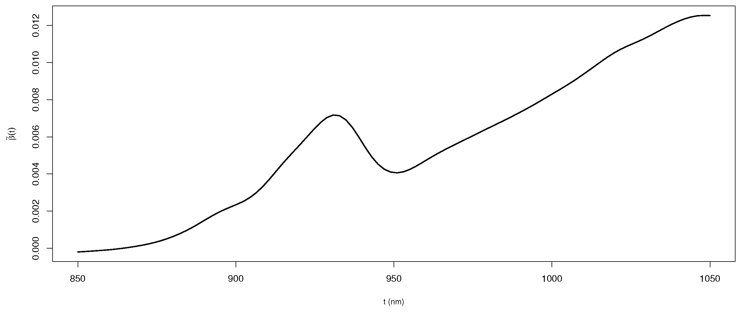
In this section, we introduce the application of the proposed estimation methods to Tecator data. The dataset is contained in the R package fda.usc in [16], and includes 215 independent food samples with fat, protein, and water of meat measured in percent. It has been widely used in the analysis of functional data. The Tecator data consist of a 100-channel spectrum of absorbances working in the wavelength from 850 to 1050 nanometers (nm). Further details on the data can be found in [2,9]. The purpose is to tease out the relation among the quantity of fatty Y (response), protein content $Z_1$, and water content $Z_2$ (real random variables), and the spectrometric curve $X\left(t\right)$ (a functional predictor). To predict the fat content of a meat sample, we consider the following PFMRM:

$$Y=\exp \left(Z_1{\alpha }_1+Z_2{\alpha }_2+{\int }_{850}^{1050}X\left(t\right)\beta \left(t\right)dt\right)ϵ.$$

(7)

To assess the predictive capability of the proposed methods, we followed [13] to randomly divide the sample into two subsamples: $I_1=\left\{(X_i,Y_i,Z_i,U_i),\left|I_1\right|=165\right\}$ as the training sample, where $|I_1|$ represents the base of $I_1$, and $I_2=\left\{(X_i,Y_i,Z_i,U_i),\left|I_2\right|=50\right\}$ as the testing sample. The training and testing samples were used to estimate parameters and check the accuracy of the prediction, respectively. We used the mean quadratic prediction error (MQEP) as a criterion to evaluate the performance of various estimation procedures. The MQEP is defined as follows:

$$\mathrm{MQEP}={\displaystyle \frac{1}{N}}\sum _{j\in I_2}{(Y_j-{\widehat{Y}}_j)}^2/{\mathrm{Var}}_{I_2}\left(Y_j\right),$$

where ${\widehat{Y}}_i$ is predicted based on the training sample, and ${\mathrm{Var}}_{I_2}$ is a response variable from test sample variance.

In addition, we compare the performances of the proposed model with the partial functional regression model in Shin [3], and log transformation on two sides of model (7) (denoted as “LogPFLM”). Specifically,

$$\begin{array}{cc}\hfill & \mathrm{PFLM}:Y=Z_1{\alpha }_1+Z_2{\alpha }_2+{\int }_{850}^{1050}X\left(t\right)\beta \left(t\right)\mathrm{d}t+e\hfill \\ \hfill & \mathrm{logPFLM}:\ln Y=Z_1{\alpha }_1+Z_2{\alpha }_2+{\int }_{850}^{1050}X\left(t\right)\beta \left(t\right)\mathrm{d}t+\epsilon \hfill \end{array}$$

The CPV criterion introduced in Section 4 was used to determine the cutoff parameter m. Here, $m=3$ was selected to explain approximately 95% of the variance in the Tecator data. Table 3 shows the average MQEP of N times repeated operations. The first and second rows of Table 3 show the prediction results of the logPFLM using LS and LAD methods, respectively. The third and fourth rows give the prediction results of (7) under the LARE and LPRE methods, respectively. The final row presents the prediction results of the PFLM without logarithmic transformation by the LS method. Overall, the LPRE outperforms all other competing methods regardless of the number of random splits. LS performs the second best, whereas LAD performs the worst. In addition, we employed the above models and methods to Tecator data just considering the scalar predictors or functional predictors; and the results indicated relatively poor performance, so we have not reported them.

Table 3. MQEP of different random partitions.

Methods	N = 100	N = 200	N = 400
LS	0.948	3.110	2.815
LAD	2.654	3.262	3.119
LARE	1.160	2.949	3.248
LPRE	0.898	2.696	1.995
PFLM	2.540	2.820	2.907

Then, we used the best-performing LPRE method to estimate the unknown parameters based on the entire dataset. The estimates of ${\alpha }_1$ and ${\alpha }_2$ are $0.102$ and $0.010$, respectively. Both protein and water are positively associated with the logarithmic transformation of fatty. Figure 1 depicts the estimated $\beta \left(t\right)$. In general, the spectrometric curve has a positive effect on the logarithmic transformation of fatty, and the estimated curve $\beta \left(t\right)$ is small due to the large integral domain. The advantages of the LPRE method are particularly evident in the analysis of this dataset.

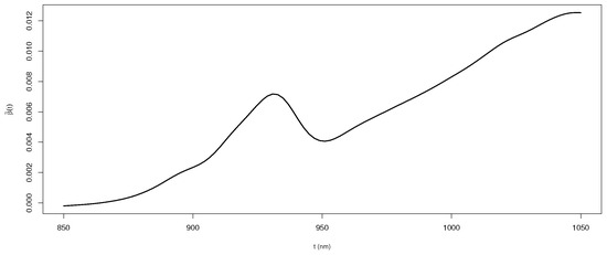
Figure 1. The estimated functional weight $\beta \left(t\right)$ in model (7) with LPRE method.

7. Conclusions

In this paper, we study the estimated problems of PFMRM based on the LARE and LPRE criteria, and the unknown slope function and functional predictor are approximated by the functional principal component analysis technique. Under some regularity conditions, we obtain the convergence rates of the slope function and the asymptotic normality of the parameter vector for two estimation methods. Both the numerical simulation results and the real data analysis show that the LPRE method is superior to the LARE, least square, and least absolute deviation methods. Several issues still warrant further study. First, we choose the Karhunen–Loève expansion to approximate the slope function in this article. Other nonparametric smoothing techniques, such as B-spline, kernel estimation, and penalty regression spline, can be used in our proposed LARE and LPRE estimation methods, and the large sample characteristics and limited sample comparison are worth studying. Furthermore, the proposed methods can also be extended to more general situations, including, but not limited to, dependent functional data, partially observed functional data, and multivariate functional data. Substantial efforts must be devoted to related advances in the future.

References

- Chen, K.; Guo, S.; Lin, Y.; Ying, Z. Least absolute relative error estimation. J. Am. Stat. Assoc. 2010, 105, 1104–1112. [Google Scholar] [CrossRef] [PubMed]
- Fan, R.; Zhang, S.; Wu, Y. Penalized relative error estimation of functional multiplicative regression models with locally sparse properties. J. Korean Stat. Soc. 2022, 51, 666–691. [Google Scholar] [CrossRef]
- Shin, H. Partial functional linear regression. J. Stat. Plan. Inference 2009, 139, 3405–3418. [Google Scholar] [CrossRef]
- Liu, C.; Su, W.; Su, W. Efficient estimation for functional accelerated failure time model. arXiv 2024, arXiv:2402.05395. [Google Scholar]
- Chen, K.; Guo, S.; Lin, Y.; Ying, Z. Least product relative error estimation. J. Multivar. Anal. 2016, 144, 91–98. [Google Scholar] [CrossRef]
- Ming, H.; Liu, H.; Yang, H. Least product relative error estimation for identification in multiplicative additive models. J. Comput. Appl. Math. 2022, 404, 113886. [Google Scholar] [CrossRef]
- Ye, F.; Zhou, H.; Yang, Y. Asymptotic properties of relative error estimation for accelerated failure time model with divergent number of parameters. Stat. Its Interface 2024, 17, 107–125. [Google Scholar] [CrossRef]
- Zhang, J.; Feng, Z.; Peng, H. Estimation and hypothesis test for partial linear multiplicative models. Comput. Stat. Data Anal. 2018, 128, 87–103. [Google Scholar] [CrossRef]
- Zhang, T.; Zhang, Q.; Li, N. Least absolute relative error estimation for functional quadratic multiplicative model. Commun. Stat.-Theory Methods 2016, 45, 5802–5817. [Google Scholar] [CrossRef]
- Zhang, T.; Huang, Y.; Zhang, Q.; Ma, S.; Ahmed, S. Penalized relative error estimation of a partially functional linear multiplicative model. In Matrices, Statistics and Big Data: Selected Contributions from IWMS 2016; Springer: Cham, Switzerland, 2019; Volume 45, pp. 127–144. [Google Scholar]
- Cai, T.; Hall, P. Prediction in functional linear regression. Ann. Stat. 2006, 34, 2159–2179. [Google Scholar] [CrossRef]
- Hall, P.; Horowitz, J.L. Methodology and convergence rates for functional linear regression. Ann. Stat. 2007, 35, 70–91. [Google Scholar] [CrossRef]
- Yu, P.; Song, X.; Du, J. Composite expectile estimation in partial functional linear regression model. J. Multivar. Anal. 2024, 203, 105343. [Google Scholar] [CrossRef]
- Xia, X.; Liu, Z.; Yang, H. Regularized estimation for the least absolute relative error models with a diverging number of covariates. Comput. Stat. Data Anal. 2016, 96, 104–119. [Google Scholar] [CrossRef]
- Tang, Q.; Cheng, L. Partial functional linear quantile regression. Sci. China Math. 2019, 57, 2589–2608. [Google Scholar] [CrossRef]
- Febrero-Bande, M.; Fuente, M. Statistical Computing in Functional Data Analysis: The R Package fda.usc. J. Stat. Softw. 2012, 51, 1–28. [Google Scholar] [CrossRef]
- Knight, K. Limiting distributions for L1 regression estimators under general conditions. Ann. Stat. 1998, 26, 755–770. [Google Scholar] [CrossRef]
- Pollard, D. Asymptotics for Least Absolute Deviations Regression Estimators. Econom. Theory 1982, 7, 186–199. [Google Scholar] [CrossRef]
Disclaimer/Publisher’s Note: The statements, opinions and data contained in all publications are solely those of the individual author(s) and contributor(s) and not of MDPI and/or the editor(s). MDPI and/or the editor(s) disclaim responsibility for any injury to people or property resulting from any ideas, methods, instructions or products referred to in the content. |
© 2025 by the authors. Licensee MDPI, Basel, Switzerland. This article is an open access article distributed under the terms and conditions of the Creative Commons Attribution (CC BY) license (https://creativecommons.org/licenses/by/4.0/).