Strict Stability of Fractional Differential Equations with a Caputo Fractional Derivative with Respect to Another Function

Abstract

In this paper, we study nonlinear systems of fractional differential equations with a Caputo fractional derivative with respect to another function (CFDF) and we define the strict stability of the zero solution of the considered nonlinear system. As an auxiliary system, we consider a system of two scalar fractional equations with CFDF and define a strict stability in the couple. We illustrate both definitions with several examples and, in these examples, we show that the applied function in the fractional derivative has a huge influence on the stability properties of the solutions. In addition, we use Lyapunov functions and their CFDF to obtain several sufficient conditions for strict stability.

1. Introduction

One of the most important ideas in the qualitative theory of differential equations is stability and there are many different types of stability defined and studied for various differential equations. Each type of stability has its own characteristics and gives some information about the behavior of the solution. The main characteristic of strict stability is concerned with the rate of decay of solutions and was introduced and studied in [1], and, later, it was generalized to impulsive systems in [2], to impulsive delay differential equations [3,4,5,6], to dynamic systems on a time scale in [7,8,9], to discrete hybrid systems in [10], to Caputo fractional differential equations in [11], and to fractional equations with non-instantaneous impulse in [12]. The most popular method for studying strict stability is via Lyapunov-type functions.

We investigate the strict stability of nonlinear fractional differential equations with the Caputo fractional derivative with respect to another function (CFDF). It is shown in examples that the applied function in the fractional derivative influences the strict stability properties of the solutions, so it gives us wider opportunities to apply this type of fractional derivative for the adequate modeling of the dynamics of real phenomena and processes. Strict stability is based on an application of appropriate Lyapunov functions and their CFDF and we present some results for exponential Lyapunov functions. As an auxiliary system, we consider a system of two scalar fractional equations with CFDF and a strict stability in the couple is defined and applied. Some comparison results are presented and sufficient conditions for strict stability are obtained. Theoretical results and definitions are illustrated with several examples.

The main contributions in this paper could be summarized as follows:

-

CFDF is applied to differential equations and strict stability is defined;

-

We prove some auxiliary properties of particular Lyapunov functions such as the exponential function;

-

We illustrate the importance of the applied function in CFDF on the behavior of solutions of the studied problem;

-

Based on examples, we consider two types of functions applied in the fractional derivatives—unbounded and bounded functions;

-

We obtain various types of sufficient conditions depending on the bounded properties of the applied functions in CFDF;

-

We illustrate the theoretical results with several examples.

2. Main Definitions from Fractional Calculus

We provide some basic definitions and properties relevant to the fractional derivatives and integrals with respect to another function [13,14,15].

Let $a\ge 0$. Throughout this paper we will assume that the function $\phi \in C^1([a,\infty ),[0,\infty ))$ and ${\phi }^{\prime }\left(t\right)>0,t\ge a$.

Definition 1 

([13]). Let $q>0$. The Riemann fractional integral with respect to another function (FIF) of the function $\upsilon :[a,\infty )\to ℝ$ is defined by (where the integral exists)

$$I_a^{q,\phi }\upsilon \left(t\right)={\displaystyle \frac{1}{\mathrm{\Gamma }\left(q\right)}}{\int }_a^t{\phi }^{\prime }\left(s\right){\left(\phi \left(t\right)-\phi \left(s\right)\right)}^{q-1}\upsilon \left(s\right)ds,t>a.$$

Definition 2 

([13]). Let $q\in (0,1)$. The Caputo fractional derivative with respect to another function (CFDF) of the function $\upsilon :[a,\infty )\to ℝ$ is defined by (where the integral exists)

$$\begin{array}{c}\hfill {}^{C}D_a^{q,\phi }\upsilon \left(t\right)={\displaystyle \frac{1}{\mathrm{\Gamma }(1-q)}}{\int }_a^t{\left(\phi \left(t\right)-\phi \left(s\right)\right)}^{-q}{\upsilon }^{\prime }\left(s\right)ds,t>a.\end{array}$$

(1)

In the case of multivalued functions, the integral FIF and the derivative CFDF are defined component-wisely.

Throughout this paper, we will assume $q\in (0,1)$.

In connection with Definition 2 and the application of CFDF, we will introduce the following sets of functions:

$$\begin{array}{cc}\hfill C^q([a,T],{ℝ}^n)& =\{\upsilon \in C([a,T],{ℝ}^n):{\upsilon }^{\prime }\mathrm{exists} \mathrm{almost} \mathrm{everywhere} \mathrm{and}\hfill \\ & \exists {}^{C}D_a^{q,\phi }\upsilon \left(t\right)\mathrm{f}\mathrm{o}\mathrm{r}t\in (a,T]\},\hfill \\ \hfill C^1([a,T],{ℝ}^n)& =\{\upsilon \in C([a,T],{ℝ}^n):{\upsilon }^{\prime }\mathrm{exists} \mathrm{and} \mathrm{it} \mathrm{is} \mathrm{continuous} \mathrm{on}[a,T]\},\hfill \end{array}$$

(2)

where $a<T\le \infty$. Note that, in the case $T=\infty$, the interval is half-open.

Remark 1. 

For a given $t>a$ in Definition 2 for the CFDF ${}^{C}D_a^{q,\phi }\upsilon \left(t\right)$ (and throughout this paper when we use it), we are assuming that the function $\upsilon \in C([a,t],{ℝ}^n),n\ge 1$, and ${\upsilon }^{\prime }$ exists almost everywhere on $[a,t]$.

In all fractional differential equations with CFDF, we will assume that their solutions are in the set $C^q([a,T],{ℝ}^n)$, $n\ge 1,T\le \infty$.

Lemma 1 

([13], (Lemma 2)). The solution of the scalar linear fractional initial value problem with CFDF

$${}^{C}D_a^{q,\phi }\upsilon \left(t\right)=\lambda \upsilon \left(t\right),\upsilon \left(a\right)={\upsilon }_0,$$

(3)

is the function

$$\upsilon \left(t\right)={\upsilon }_0{E}_q\left(\lambda {(\phi \left(t\right)-\phi \left(a\right))}^q\right),$$

(4)

where $\lambda \in ℝ$ is a given constant and $E_q(.)$ is the Mittag-Leffler function of one parameter.

Proposition 1. 

Let $\upsilon \in C^q([a,T],ℝ)$, $a<T\le \infty ,$ be an increasing function. Then, ${}^{C}D_a^{q,\phi }{e}^{\upsilon \left(t\right)}\ge 0$ holds for all $t\in (a,T]$.

The proof follows from the definition of CFDF so we omit it.

We now introduce the following assumptions:

(A1).

The function $\phi \in C^1([a,\infty ),[0,\infty ))$, ${\phi }^{\prime }\left(t\right)>0$ for $t\ge a,$ and ${lim}_{t\to \infty }\phi \left(t\right)=\infty$;

(A2).

The function $\phi \in C^1([a,\infty ),[0,\infty ))$, ${\phi }^{\prime }\left(t\right)>0$ for $t\ge a,$ and $\phi \left(t\right)\le L,t\ge a$ with $L>0$ being a constant.

Remark 2. 

For example, the function $\phi \left(t\right)=t^2+t$ satisfies assumption (A1) on $[0,\infty )$ and the function $\phi \left(t\right)={\displaystyle \frac{t+1}{t+2}}$ satisfies assumption (A2) on $[0,\infty )$.

The function $\phi (.)$ applied in Caputo-type fractional derivative CFDF influences the behavior of the solutions of the differential equations with CFDF. For example, we consider the scalar linear differential Equation (3) with a solution given by (4) (see Lemma 1). The conditions (A1) and (A2) of the function $\phi (.)$ have a huge influence on the behavior of Mittag-Leffler functions, and, respectively, on the solution of (3). We will give the following results, whose proofs are obvious (so we will omit them) and we will illustrate them only on some graphs (see Figure 1, Figure 2, Figure 3 and Figure 4).

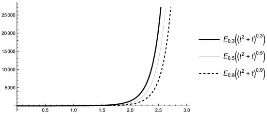
Figure 1. Graphs of $E_q\left({(\phi \left(t\right)-\phi \left(0\right))}^q\right)$ for $\phi \left(t\right)=t^2+t$ and various $q=0.3,q=0.5,q=0.9$.

Figure 2. Graphs of $E_q(-{(\phi \left(t\right)-\phi \left(0\right))}^q)$ for $\phi \left(t\right)=t^2+t$ and various $q=0.3,q=0.5,q=0.9$.

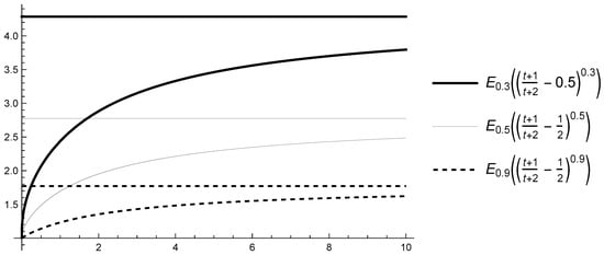
Figure 3. Graphs of $E_q\left({(\phi \left(t\right)-\phi \left(0\right))}^q\right)$ and their limits $E_q\left({(L-\phi \left(0\right))}^q\right)$ for $\phi \left(t\right)={\displaystyle \frac{t+1}{t+2}}$, $L=1$, and various $q=0.3,q=0.5,q=0.9$.

Figure 4. Graphs of $E_q(-{(\phi \left(t\right)-\phi \left(0\right))}^q)$ and their limits $E_q(-{(L-\phi \left(0\right))}^q)$ for $\phi \left(t\right)={\displaystyle \frac{t+1}{t+2}}$, $L=1$, and various $q=0.3,q=0.5,q=0.9$.

Proposition 2. 

The following results are true:

-

If assumption (A1) is satisfied and $\lambda >0$, then $E_q\left(\lambda {(\phi \left(t\right)-\phi \left(a\right))}^q\right)$ is an increasing function and ${lim}_{t\to \infty }{E}_q\left(\lambda {(\phi \left(t\right)-\phi \left(a\right))}^q\right)=\infty$ (see Figure 1 for $\lambda =1$ and $a=0$). Thus, the solution (4) of the scalar linear differential equation with CFDF (3) satisfies ${lim}_{t\to \infty }\upsilon \left(t\right)=\infty .$

-

If assumption (A1) is satisfied and $\lambda <0$, then $E_q\left(\lambda {(\phi \left(t\right)-\phi \left(a\right))}^q\right)$ is a decreasing function and ${lim}_{t\to \infty }{E}_q\left(\lambda {(\phi \left(t\right)-\phi \left(a\right))}^q\right)=0$ (see Figure 2 for $\lambda =-1$ and $a=0$). Thus, the solution (4) of the scalar linear differential equation with CFDF (3) satisfies ${lim}_{t\to \infty }\upsilon \left(t\right)=0$.

-

If assumption (A2) is satisfied and $\lambda >0$, then $E_q\left(\lambda {(\phi \left(t\right)-\phi \left(0\right))}^q\right)$ is an increasing function and ${lim}_{t\to \infty }{E}_q\left(\lambda {(\phi \left(t\right)-\phi \left(a\right))}^q\right)=E_q\left(\lambda {(L-\phi \left(a\right))}^q\right)$ (see Figure 3 for $\lambda =1$ and $a=0$). Thus, the solution (4) of the scalar linear differential equation with CFDF (3) satisfies ${lim}_{t\to \infty }\upsilon \left(t\right)={\upsilon }_0{E}_q\left(\lambda {(L-\phi \left(a\right))}^q\right).$

-

If assumption (A2) is satisfied and $\lambda <0$, then $E_q\left(\lambda {(\phi \left(t\right)-\phi \left(a\right))}^q\right)$ is a decreasing function and ${lim}_{t\to \infty }{E}_q\left(\lambda {(\phi \left(t\right)-\phi \left(a\right))}^q\right)=E_q\left(\lambda {(L-\phi \left(a\right))}^q\right)$ (see Figure 4 for $\lambda =-1$ and $a=0$). Thus, the solution (4) of the scalar linear differential equation with CFDF (3) satisfies ${lim}_{t\to \infty }\upsilon \left(t\right)={\upsilon }_0{E}_q\left(\lambda {(L-\phi \left(a\right))}^q\right).$

Remark 3. 

In the case $\phi \left(t\right)=t$, the above-defined FIF and CFDF coincide with the classical definitions of the Riemann fractional integral and the Caputo fractional derivative ([14]). Also, in this case, assumption (A1) is satisfied; the solution of the corresponding scalar linear fractional differential equation with CFDF satisfies ${lim}_{t\to \infty }\upsilon \left(t\right)=\infty$ (with $\lambda >0$) or ${lim}_{t\to \infty }\upsilon \left(t\right)=0$ (with $\lambda <0$) (see, for example, [14]).

We now prove a result for CFDF.

Lemma 2. 

Let $\upsilon :[a,T]\to ℝ$, $a<T\le \infty$ and there exists a point $\xi \in (a,T]$ such that $\upsilon \left(\xi \right)=0$, and $\upsilon \left(t\right)<0$, for $t\in [a,\xi )$ and the CFDF ${}^{C}D_a^{q,\phi }{\upsilon \left(t\right)|}_{t=\xi }$ exists. Then, if ${lim}_{s\to \xi -}\left({\displaystyle \frac{v\left(s\right)}{{(\phi \left(\xi \right)-\phi \left(s\right))}^q}}\right)=0$, we have ${}^{C}D_a^{q,\phi }{\upsilon \left(t\right)|}_{t=\xi }\ge 0$.

Proof. 

Apply ${\displaystyle \frac{{\upsilon }^{\prime }\left(s\right)}{{\left(\phi \left(\xi \right)-\phi \left(s\right)\right)}^q}}={\displaystyle \frac{d}{ds}}\left({\displaystyle \frac{\upsilon \left(s\right)}{{\left(\phi \left(\xi \right)-\phi \left(s\right)\right)}^q}}\right)-{\displaystyle \frac{q{\phi }^{\prime }\left(s\right)\upsilon \left(s\right)}{{\left(\phi \left(\xi \right)-\phi \left(s\right)\right)}^{1+q}}},\mathrm{a}.\mathrm{e}.s\in (a,\xi )$ and integration by parts to (1) and obtain

$$\begin{array}{cc}\hfill {}^{C}D_a^{q,\phi }{\upsilon \left(t\right)|}_{t=\xi }& ={\displaystyle \frac{1}{\mathrm{\Gamma }(1-q)}}{\int }_a^{\xi }{\left(\phi \left(\xi \right)-\phi \left(s\right)\right)}^{-q}{\upsilon }^{\prime }\left(s\right)ds\hfill \\ & ={\displaystyle \frac{1}{\mathrm{\Gamma }(1-q)}}{\int }_a^{\xi }{\displaystyle \frac{d}{ds}}\left({\displaystyle \frac{\upsilon \left(s\right)}{{\left(\phi \left(\xi \right)-\phi \left(s\right)\right)}^q}}\right)ds\hfill \\ & -{\displaystyle \frac{q}{\mathrm{\Gamma }(1-q)}}{\int }_a^{\xi }{\displaystyle \frac{{\phi }^{\prime }\left(s\right)\upsilon \left(s\right)}{{\left(\phi \left(\xi \right)-\phi \left(s\right)\right)}^{1+q}}}ds\hfill \\ & =-{\displaystyle \frac{1}{\mathrm{\Gamma }(1-q)}}\left({\displaystyle \frac{\upsilon \left(a\right)}{{\left(\phi \left(\xi \right)-\phi \left(a\right)\right)}^q}}\right)-{\displaystyle \frac{q}{\mathrm{\Gamma }(1-q)}}{\int }_a^{\xi }{\displaystyle \frac{{\phi }^{\prime }\left(s\right)\upsilon \left(s\right)}{{\left(\phi \left(\xi \right)-\phi \left(s\right)\right)}^{1+q}}}ds.\hfill \end{array}$$

(5)

From (5), and $\upsilon \left(s\right)\le 0,{\phi }^{\prime }\left(s\right)>0$ for $s\in [a,\xi ],$ we have the claim in Lemma 2. □

Corollary 1. 

Let $\upsilon :[a,T]\to ℝ$, $a<T\le \infty$ and there exists a point $\xi \in (a,T]$ such that $\upsilon \left(\xi \right)=0$, and $\upsilon \left(t\right)>0$, for $t\in [a,\xi )$, and the CFDF ${}^{C}D_a^{q,\phi }{\upsilon \left(t\right)|}_{t=\xi }$ exists. Then, if ${lim}_{s\to \xi -}\left({\displaystyle \frac{v\left(s\right)}{{(\phi \left(\xi \right)-\phi \left(s\right))}^q}}\right)=0$, we have ${}^{C}D_a^{q,\phi }{\upsilon \left(t\right)|}_{t=\xi }\le 0$.

Remark 4. 

In Lemma 2 and Corollary 1, if $\upsilon \in C^1([a,T],ℝ)$, then L’Hopital’s rule guarantees that ${lim}_{s\to \xi -}\left({\displaystyle \frac{\upsilon \left(s\right)}{{(\phi \left(\xi \right)-\phi \left(s\right))}^q}}\right)={lim}_{s\to \xi -}{\displaystyle \frac{{\upsilon }^{\prime }\left(s\right)}{-q{\phi }^{\prime }\left(s\right)}}{(\phi \left(\xi \right)-\phi \left(s\right))}^{1-q}=0,$ i.e., ${lim}_{s\to \xi -}\left({\displaystyle \frac{\upsilon \left(s\right)}{{(\phi \left(\xi \right)-\phi \left(s\right))}^q}}\right)=0$ is automatically true. Of course, one could also put other conditions (other than $\upsilon \in C^1([a,T],ℝ)$; for example, instead, one could assume ${lim}_{s\to \xi -}{\upsilon }^{\prime }\left(s\right)$ exists and is a real number) to guarantee that this limit is zero.

3. Statement of the Problem and Some Preliminary Results

Consider the initial value problem (IVP) for the nonlinear system of fractional differential equations with CFDF for $q\in (0,1)$:

$${}^{C}D_a^{q,\phi }y\left(t\right)=f(t,y\left(t\right)),y\left(a\right)=y_0$$

(6)

where $y_0\in {ℝ}^n,f\in C([a,\infty )\times {ℝ}^n,{ℝ}^n)$.

We will study strict stability for (6) and, in connection with this, we will assume $f(t,0)=0,t\ge a$. Also, we will assume the function $f\in C([a,\infty )\times {ℝ}^n,{ℝ}^n)$ is such that, for any initial data $(a,y_0)\in [0,\infty )\times {ℝ}^n$, the IVP (6) has a solution $y(t;a,y_0)\in C^q([a,\infty ),{ℝ}^n)$.

We will use Lyapunov-like functions to investigate the strict stability of the system of differential equations with CFDF (6). In connection with this, we will use the following class of functions:

Definition 3. 

Let $\mathrm{\Sigma }\subset {ℝ}^n,0\in \mathrm{\Sigma }$. We say that the function $V(.):\mathrm{\Sigma }\to [0,\infty )$ belongs to the class $\mathrm{\Omega }\left(\mathrm{\Sigma }\right)$ if $V(.)\in C(\mathrm{\Sigma },[0,\infty \left)\right)$ is continuously differentiable in Σ.

Remark 5. 

Let $x\in {ℝ}^n,x=(x_1,x_2,\cdots ,x_n)$. The functions $V\left(x\right)={\sum }_{i=1}^n{x}_i^2,V\left(x\right)={\sum }_{i=1}^n\left|x_i\right|,V\left(x\right)={\sum }_{i=1}^n{e}^{x_i},V\left(x\right)={\sum }_{i=1}^n{e}^{-x_i},V\left(x\right)=e^{{\sum }_{i=1}^n{x}_i},$ and $V\left(x\right)=e^{-{\sum }_{i=1}^n{x}_i}$, for example, are from the class $\mathrm{\Omega }\left(\mathrm{\Sigma }\right)$.

We now use the following comparison results for Lyapunov functions and their CFDF. For this purpose, we consider the IVP for the nonlinear scalar fractional differential equation with CFDF:

$${}^{C}D_a^{q,\phi }\upsilon \left(t\right)=g(t,\upsilon ),\upsilon \left(a\right)={\upsilon }_0$$

(7)

where ${\upsilon }_0\in ℝ,g\in C([a,\infty )\times ℝ,ℝ)$, $g(t,0)\equiv 0$, $t\ge a$.

Lemma 3. 

We assume the following:

1. The function $y^{\ast }\left(t\right)=y(t;a,y_0),y^{\ast }\in C^q([a,T],\mathrm{\Sigma })\cap C^1([a,T],\mathrm{\Sigma })$ is a solution of (6) where $\mathrm{\Sigma }\subset {ℝ}^n,0\in \mathrm{\Sigma }$, $T:a<T\le \infty$ is a given constant, $y_0\in \mathrm{\Sigma }$.

2. Let ${\upsilon }_0\in ℝ$ be a given point and there exists a number $L>0$ such that, for any $\eta \in ℝ:\left|\eta \right|<L$, the initial value problem for the scalar fractional differential equation with CFDF

$${}^{C}D_a^{q,\phi }\omega \left(t\right)=g\left(t,\omega \right)+\eta ,\omega \left(a\right)={\upsilon }_0+\eta$$

(8)

has a unique solution ${\omega }_{\eta }(.)\in C^q([a,T],ℝ)\cap C^1([a,T],ℝ)$.

3. The function $V\in \mathrm{\Omega }\left(\mathrm{\Sigma }\right)$, $V\left(y^{\ast }(.)\right)\in C^q([a,T],ℝ)$ and the inequality

$${}^{C}D_a^{q,\phi }V\left(y^{\ast }\left(t\right)\right)\le (\ge )g(t,V\left(y^{\ast }\left(t\right)\right)),$$

holds.

Then, $V\left(y_0\right)\le (\ge ){\upsilon }_0$ implies the inequality $V\left(y^{\ast }\left(t\right)\right)\le (\ge ){\upsilon }^{\ast }\left(t\right)$ for $t\in [a,T],$ where ${\upsilon }^{\ast }(.)\in C^q([a,T],ℝ)\cap C^1([a,T],ℝ)$ is the unique solution of (8) with $\eta =0$.

Proof. 

Case 1. Suppose the inequalities

$${}^{C}D_a^{q,\phi }V\left(y^{\ast }\left(t\right)\right)\le g(t,V\left(y^{\ast }\left(t\right)\right)),t\in (a,T]$$

(9)

and ${\upsilon }_0\ge V\left(y_0\right)$ hold.

According to condition 2 of Lemma 3, for an arbitrary number $\eta \in (0,L)$, there exists a unique solution ${\omega }_{\eta }\left(t\right)$ of (8) with initial condition ${\omega }_0={\upsilon }_0+\eta$.

Consider the function $\mu \left(t\right)=V\left(y^{\ast }\left(t\right)\right)\in C^q([a,T],ℝ)\cap C^1([a,T],ℝ).$ Note $\mu \left(a\right)=V\left(y^{\ast }\left(a\right)\right)\le {\upsilon }_0<{\upsilon }_0+\eta ={\omega }_{\eta }\left(a\right)$. We now prove the inequality

$$\mu \left(t\right)<{\omega }_{\eta }\left(t\right)\mathrm{f}\mathrm{o}\mathrm{r}t\in [a,T].$$

(10)

Assume $\exists \xi \in (a,T):\mu \left(\xi \right)={\omega }_{\eta }\left(\xi \right)$ and $\mu \left(t\right)<{\omega }_{\eta }\left(t\right)$ on $[a,\xi )$.

According to Lemma 2 and Remark 4, for the point $\xi \in (a,T)$ and the function $\mu \left(t\right)-{\omega }_{\eta }\left(t\right),t\in [a,\xi ]$, we obtain ${}^{C}D_a^{q,\phi }\left(\mu \left(t\right)-{\omega }_{\eta }\left(t\right)\right){|}_{t=\xi }\ge 0$, i.e.,

$${}^{C}D_a^{q,\phi }\mu \left(t\right){{|}_{t=\xi }\ge {}^{C}D_a^{q,\phi }{\omega }_{\eta }\left(t\right)|}_{t=\xi }=g(\xi ,{\omega }_{\eta }\left(\xi \right))+\eta >g(\xi ,{\omega }_{\eta }\left(\xi \right))=g(\xi ,m\left(\xi \right)).$$

According to inequality (9), for $t=\xi$ we have ${}^{C}D_a^{q,\phi }{\mu \left(t\right)|}_{t=\xi }={}^{C}D_a^{q,\phi }V\left(y^{\ast }\left(t\right)\right){|}_{t=\xi }\le g(\xi ,V\left(y^{\ast }\left(\xi \right)\right)=g(\xi ,\mu \left(\xi \right))$. The obtained contradiction proves inequality (10).

Since inequality (10) is satisfied, for any $\eta \in (0,L]$ after taking the limit as $\eta \to 0$, we obtain $V\left(y^{\ast }\left(t\right)\right)=\mu \left(t\right)\le {\omega }_{\eta }{\left(t\right)|}_{\eta =0}={\upsilon }^{\ast }\left(t\right),t\in [a,T].$

Case 2. Suppose the inequalities

$${}^{C}D_a^{q,\phi }V\left(y^{\ast }\left(t\right)\right)\ge g(t,V\left(y^{\ast }\left(t\right)\right)),t\in (a,T]$$

(11)

and $V\left(y_0\right)\ge {\upsilon }_0$ hold. The proof of the claim is similar to the one in Case 1 where $\eta \in (-L,0]$ and we apply Corollary 1 instead of Lemma 2. □

Remark 6. 

If, in Lemma 3, we do not assume $y^{\ast }$ is in $C^1([a,T],\mathrm{\Sigma })$ and ${\omega }_{\eta }(.)$ is in $C^1([a,T],ℝ)$, then, to apply Lemma 2 above, in the proof, we would need the following condition:

For any fixed $\eta \in ℝ:\left|\eta \right|<L$ if $\exists \xi \in (a,T]:V\left(y^{\ast }\left(\xi \right)\right)={\omega }_{\eta }\left(\xi \right)$, then ${lim}_{s\to \xi -}\left({\displaystyle \frac{V\left(y^{\ast }\left(s\right)\right)-{\omega }_{\eta }\left(s\right)}{{(\phi \left(\xi \right)-\phi \left(s\right))}^q}}\right)=0$.

As a partial case of Lemma 3, we obtain the following result:

Corollary 2. 

We assume the following:

1. The function $y^{\ast }\left(t\right)=y(t;a,y_0),y^{\ast }\in C^q([a,T],\mathrm{\Sigma })\cap C^1([a,T],\mathrm{\Sigma }),$ is a solution of (6) where $\mathrm{\Sigma }\subset {ℝ}^n,0\in \mathrm{\Sigma }$, $T>a$, $y_0\in \mathrm{\Sigma }$.

2. The function $V\in \mathrm{\Omega }\left(\mathrm{\Sigma }\right),V\left(y^{\ast }(.)\right)\in C^q([a,T],ℝ)$, and the inequality

$${}^{C}D_a^{q,\phi }V\left(y^{\ast }\left(t\right)\right)\le (\ge )0,t\in (a,T]$$

holds.

Then, the inequality $V\left(y^{\ast }\left(t\right)\right)\le (\ge )V\left(y_0\right),t\in [a,T],$ holds.

The proof of Corollary 2 follows from Lemma 3 with $g(t,\upsilon )\equiv 0$ and ${\upsilon }_0=V\left(y_0\right)$ and we omit it.

For the exponential Lyapunov function, we obtain the following comparison result:

Corollary 3. 

We assume the following:

1. The function $y^{\ast }\left(t\right)=y(t;a,y_0),y^{\ast }\in C^q([a,T],\mathrm{\Sigma })\cap C^1([a,T],\mathrm{\Sigma }),y^{\ast }=(y_1^{\ast },y_2^{\ast },\cdots ,y_n^{\ast }),$ is a solution of (6) with $\mathrm{\Sigma }\subset {ℝ}^n,0\in \mathrm{\Sigma }$, $a,T\in [0,\infty ):a<T$, $y_0\in \mathrm{\Sigma }$.

2. The inequality

$${}^{C}D_a^{q,\phi }{e}^{\varsigma {\sum }_{i=1}^n{y}_i^{\ast }\left(t\right)}\le (\ge )K\sum _{i=1}^n{y}_i^{\ast }\left(t\right),t>a$$

holds where $\varsigma \in ℝ,K>0$.

Then, the inequality $e^{\varsigma {\sum }_{i=1}^n{y}_i^{\ast }\left(t\right)}\le (\ge )E_q\left(K{(\phi \left(t\right)-\phi \left(a\right))}^q\right)e^{\varsigma {\sum }_{i=1}^n{y}_{0,i}}$ holds for $t\in [a,T].$

Proof. 

In this case, $V\left(y\right)=e^{\varsigma {\sum }_{i=1}^n{y}_i}>0$ for $y\in {ℝ}^n,y=(y_1,y_2,\cdots ,y_n)$ is a differentiable function. The unique solution of (8) with $g(t,\omega )=K\omega$ and $\eta =0$ is $\omega \left(t\right)={\upsilon }_0{E}_q\left(K{(\phi \left(t\right)-\phi \left(a\right))}^q\right)$ (see Lemma 1). Then, according to Lemma 3 with $g(t,\omega )=K\omega$ and ${\upsilon }_0=V\left(y_0\right)=e^{\varsigma {\sum }_{i=1}^n{y}_{0,i}},$ the inequality $e^{\varsigma {\sum }_{i=1}^n{y}_i^{\ast }\left(t\right)}\le (\ge )E_q\left(K{(\phi \left(t\right)-\phi \left(a\right))}^q\right)e^{\varsigma {\sum }_{i=1}^n{y}_{0,i}},t\in [a,T]$ holds. □

Remark 7. 

The function $\phi (.)$ influences the behavior of the solutions of fractional differential equations with CFDF. Let $y^{\ast }\left(t\right)$ be a solution of (6) Then, we have the following:

-

Let assumption (A1) be fulfilled with $T=\infty$ and ${}^{C}D_a^{q,\phi }{e}^{{\sum }_{i=1}^n{y}_i^{\ast }\left(t\right)}\ge K{\sum }_{i=1}^n{y}_i^{\ast }\left(t\right)$. According to Corollary 3 with $\varsigma =1$, it follows that $e^{{\sum }_{i=1}^n{y}_i^{\ast }\left(t\right)}\ge E_q\left(K{(\phi \left(t\right)-\phi \left(a\right))}^q\right)e^{{\sum }_{i=1}^n{y}_{0,i}}$ and, from $\left|\right|y^{\ast }\left(t\right)\left|\right|={\sum }_{i=1}^n\left|y_i^{\ast }\left(t\right)\right|\ge {\sum }_{i=1}^n{y}_i^{\ast }\left(t\right)$ and ${lim}_{t\to \infty }{E}_q\left(t^q\right)=+\infty$, we obtain ${lim}_{t\to \infty }\left|\right|y^{\ast }\left(t\right)\left|\right|=\infty$.

-

Let assumption (A2) be fulfilled with $T=\infty$ and ${}^{C}D_a^{q,\phi }{e}^{{\sum }_{i=1}^n{y}_i^{\ast }\left(t\right)}\ge K{\sum }_{i=1}^n{y}_i^{\ast }\left(t\right)$. From Corollary 3 with $\varsigma =1$, it follows that $e^{{\sum }_{i=1}^n{y}_i^{\ast }\left(t\right)}\ge E_q\left(K{(\phi \left(t\right)-\phi \left(a\right))}^q\right)e^{{\sum }_{i=1}^n{y}_{0,i}}\ge e^{{\sum }_{i=1}^n{y}_{0,i}}$ and

$$\left|\right|y^{\ast }\left(t\right)\left|\right|=\sum _{i=1}^n\left|y_i^{\ast }\left(t\right)\right|\ge \sum _{i=1}^n{y}_i^{\ast }\left(t\right)\ge \sum _{i=1}^n{y}_{0,i},t\ge a.$$

-

Let assumption (A2) be fulfilled with $T=\infty$ and ${}^{C}D_a^{q,\phi }{e}^{{\sum }_{i=1}^n{y}_i^{\ast }\left(t\right)}\le K{\sum }_{i=1}^n{y}_i^{\ast }\left(t\right)$. From Corollary 3 with $\varsigma =1$, it follows that

$$e^{{\sum }_{i=1}^n{y}_i^{\ast }\left(t\right)}\le E_q\left(K{(\phi \left(t\right)-\phi \left(a\right))}^q\right)e^{{\sum }_{i=1}^n{y}_{0,i}}\le E_q\left(K{(L-\phi \left(a\right))}^q\right)e^{{\sum }_{i=1}^n{y}_{0,i}}$$

and

$$\left|\right|y^{\ast }\left(t\right)\left|\right|=\sum _{i=1}^n\left|y_i^{\ast }\left(t\right)\right|\le ln\left(E_q\left(K{(L-\phi \left(a\right))}^q\right)e^{{\sum }_{i=1}^n{y}_{0,i}}\right),t\ge a,$$

i.e., the norm of the solution is bounded from above.

-

Let assumption (A2) be satisfied, $T=\infty$ and ${}^{C}D_a^{q,\phi }{e}^{-{\sum }_{i=1}^n{y}_i^{\ast }\left(t\right)}\le K{\sum }_{i=1}^n{y}_i^{\ast }\left(t\right)$. Then, from Corollary 3 with $\varsigma =-1$, it follows that

$$e^{-{\sum }_{i=1}^n{y}_i^{\ast }\left(t\right)}\le E_q\left(K{(\phi \left(t\right)-\phi \left(a\right))}^q\right)e^{-{\sum }_{i=1}^n{y}_{0,i}}\le E_q\left(K{(L-\phi \left(a\right))}^q\right)e^{-{\sum }_{i=1}^n{y}_{0,i}}$$

and $e^{-\left|\right|y_i^{\ast }\left(t\right)\left|\right|}=e^{-{\sum }_{i=1}^n\left|y_i^{\ast }\left(t\right)\right|}\le e^{-{\sum }_{i=1}^n{y}_i^{\ast }\left(t\right)}\le E_q\left(K{(L-\phi \left(a\right))}^q\right)e^{-{\sum }_{i=1}^n{y}_{0,i}}$ or $\left|\right|y\left(t\right)\left|\right|\ge ln\left({\displaystyle \frac{e^{{\sum }_{i=1}^n{y}_{0,i}}}{E_q\left(K{(L-\phi \left(a\right))}^q\right)}}\right)$, i.e., the norm of the solution has a lower bound depending on its initial value.

Proposition 3. 

Let condition 2 of Lemma 3 be satisfied. If ${\upsilon }_0>0$, then the solution $\upsilon (t;a,{\upsilon }_0)$ of (8) with $\eta =0$ is nonnegative.

Proof. 

Let $\eta \in (0,L)$ and ${\upsilon }_0>0$. Then, ${\omega }_0={\upsilon }_0+\eta >{\upsilon }_0>0$. Let ${\omega }_{\eta }\left(t\right)$ be the unique solution of (8) with the initial value ${\upsilon }_0+\eta$. We will prove the inequality

$${\omega }_{\eta }\left(t\right)>0,t\in [a,T].$$

(12)

Assume there exists $\xi \in (a,T)$ such that ${\omega }_{\eta }\left(\xi \right)=0$ and ${\omega }_{\eta }\left(t\right)>0$ on $[0,\xi )$. According to Corollary 1 and Remark 4, the inequality ${}^{C}D_a^{q,\phi }{\omega }_{\eta }{\left(t\right)|}_{t=\xi }\le 0$ holds, or $0\ge {}^{C}D_a^{q,\phi }{\omega }_{\eta }{\left(t\right)|}_{t=\xi }=g(\xi ,{\omega }_{\eta }\left(\xi \right))+\eta =g(\xi ,0)+\eta >g(\xi ,0)$. The obtained contradiction proves the validity of inequality (12). We take a limit as $\eta \to 0$ in inequality (12) and obtain $\upsilon (t;a,{\upsilon }_0)={\omega }_0\left(t\right)\ge 0,t\in [a,T]$. □

4. Strict Stability

We define strict stability for fractional differential equations with CFDF using the idea for ordinary differential equations (see, for example, [1]).

Definition 4. 

The system of fractional differential equations with CFDF (6) is said to be strictly stable if, for a given ${ϵ}_1>0$, there exists ${\delta }_1={\delta }_1(a,{ϵ}_1)>0$ and, for any ${\delta }_2={\delta }_2(a,{ϵ}_1),{\delta }_2\in (0,{\delta }_1)$, there exists ${ϵ}_2={ϵ}_2(a,{\delta }_2)\in (0,{\delta }_2)$ such that the inequality ${\delta }_2<\left|\right|y_0\left|\right|<{\delta }_1$ implies ${ϵ}_2<\left|\right|y(t;a,y_0)\left|\right|<{ϵ}_1$ for $t\ge a$ where $y(t;a,y_0)$ is a solution of (6).

Remark 8. 

Note that, if the zero solution is strictly stable, then it does not approach zero as we go to infinity.

Example 1. 

(Strict stability). Consider the scalar linear fractional differential equation with CFDF

$${}^{C}D_0^{0.3,\phi }\upsilon \left(t\right)=\lambda \upsilon ,\upsilon \left(0\right)=x_0$$

(13)

with a solution (see Lemma 1) $\upsilon \left(t\right)=x_0{E}_{\mathcal{A}}\left(\lambda {(\phi \left(t\right)-\phi \left(0\right))}^{0.3}\right)$.

Case 1. Let $\lambda =1$ and $\phi \left(t\right)={\displaystyle \frac{t+1}{t+2}},t\ge 0$, i.e., assumption (A2) is satisfied with $L=1$. Since $1=E_{0.3}\left(0\right)\le E_{0.3}\left({({\displaystyle \frac{t+1}{t+2}}-0.5)}^{0.3}\right)<E_{0.3}(0.5^{0.3})$ for $t\ge 0$, it follows that, for any ${\epsilon }_1$, if $|x_0| <{\delta }_1={\displaystyle \frac{{\epsilon }_1}{E_{0.3}(0.5^{0.3})}}$, then $\left|\upsilon \left(t\right)\right|<{\epsilon }_1$, and, for any ${\delta }_2\in (0,{\delta }_1)=\left(0,{\displaystyle \frac{{\epsilon }_1}{E_{0.3}(0.5^{0.3})}}\right)$, if ${\epsilon }_2=0.5{\delta }_2<{\delta }_2$, the inequality $|x_0|>{\delta }_2$ implies $\left|\upsilon \left(t\right)\right|>{\delta }_2>{\epsilon }_2$. Therefore, the scalar linear fractional differential equation with CFDF (13) is strictly stable (see Figure 5).

Figure 5. Graphs of the solutions of (13) with $\lambda =1$, $\phi \left(t\right)={\displaystyle \frac{t+1}{t+2}},t\ge 0$ and various initial values $x_0$.

Case 2. Let $\lambda =-1$ and $\phi \left(t\right)={\displaystyle \frac{t+1}{t+2}},t\ge 0$, i.e., assumption (A2) is satisfied with $L=1$. Since $E_{0.3}(-0.5^{0.3})<E_{0.3}(-{({\displaystyle \frac{t+1}{t+2}}-0.5)}^{0.3})\le 1$ for $t\ge 0$, it follows that, for any ${\epsilon }_1$ if $|x_0|<{\delta }_1={\epsilon }_1$ then $\left|\upsilon \left(t\right)\right|<{\epsilon }_1$, and for any ${\delta }_2\in (0,{\delta }_1)=(0,{\epsilon }_1)$, if ${\epsilon }_2=E_{0.3}(-0.5^{0.3}){\delta }_2<{\delta }_2$, then the inequality $|x_0|>{\delta }_2$ implies $\left|\upsilon \left(t\right)\right|>{\delta }_2{E}_{0.3}(-0.5^{0.3})={\epsilon }_2$. Therefore, the scalar fractional differential equation with CFDF (13) is strictly stable (see Figure 6).

Figure 6. Graphs of the solutions of (13) with $\lambda =-1$, $\phi \left(t\right)={\displaystyle \frac{t+1}{t+2}},t\ge 0$ and various initial values $x_0$.

Case 3. Let $\lambda =1$ and $\phi \left(t\right)=t^2+t,t\ge 0$, i.e., assumption (A1) is satisfied. Then, the solution is $x\left(t\right)=x_0{E}_{0.3}\left({(t^2+t)}^{0.3}\right)$. Since $E_{0.3}\left({(t^2+t)}^{0.3}\right)$ is an increasing function approaching infinity, the solution of (13) is not strictly stable (see Figure 7).

Figure 7. Graphs of the solutions of (13) with $\lambda =1$, $\phi \left(t\right)=t^2+t,t\ge 0$ and various initial values $x_0$.

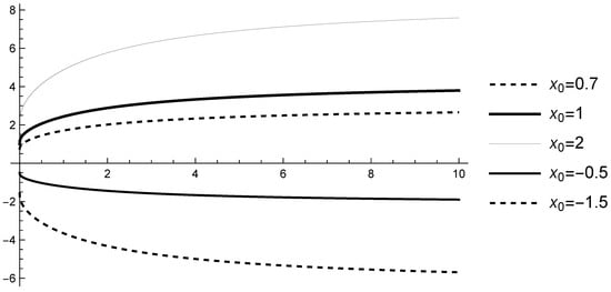
Case 4. Let $\lambda =-1$ and $\phi \left(t\right)=t^2+t,t\ge 0$, i.e., assumption (A1) is satisfied. Since $E_{0.3}(-{(t^2+t)}^{0.3})\le E_{0.3}\left(0\right)$ is a decreasing function approaching zero at infinity, the solution $\upsilon \left(t\right)=x_0{E}_{0.3}(-{(t^2+t)}^{0.3})$ of (13) approaches zero at infinity but it is not strictly stable. The initial value has an influence only on the rate of approaching 0 (see Figure 8).

Figure 8. Graphs of the solutions of (13) with $\lambda =-1$, $\phi \left(t\right)=t^2+t,t\ge 0$ and various initial values $x_0$.

Example 1 illustrates the influence of the applied function in the fractional derivative on the stability properties of the studied equation.

We now consider a couple of fractional differential equations with CFDF:

$$\begin{array}{cc}& {}^{C}D_a^{q,\phi }\upsilon ={\mathcal{T}}_1\left(t,\upsilon \left(t\right)\right)\mathrm{for}t>a,\upsilon \left(a\right)={\upsilon }_0,\hfill \\ & {}^{C}D_a^{q,\phi }\omega ={\mathcal{T}}_2\left(t,\omega \left(t\right)\right)\mathrm{for}t>a,\omega \left(a\right)={\omega }_0,\hfill \end{array}$$

(14)

where ${\upsilon }_0,{\omega }_0\in ℝ$, ${\mathcal{T}}_1,{\mathcal{T}}_2:{ℝ}_{+}\times ℝ\to ℝ$, ${\mathcal{T}}_i(t,0)\equiv 0,$ and $i=1,2$.

We will define the strict stability of the couple of fractional differential equations with CFDF.

Definition 5. 

The couple of scalar equations with CFDF (14) is strictly stable in the couple if, for a given ${ϵ}_1>0$, there exists ${\delta }_1={\delta }_1\left({ϵ}_1\right)>0$ and, for any ${\delta }_2={\delta }_2\left({ϵ}_1\right)\in (0,{\delta }_1)$, there exists ${ϵ}_2={ϵ}_2\left({\delta }_2\right)\in (0,{\delta }_2)$ such that the inequalities $|{\upsilon }_0|<{\delta }_1$ and ${\delta }_2<\left|{\omega }_0\right|$ imply $|\upsilon (t;a,{\upsilon }_0)|<{ϵ}_1$ and ${ϵ}_2<\left|\omega (t;a,{\omega }_0)\right|$ for $t\ge a$ where the couple of functions $\left(\upsilon (t;a,{\upsilon }_0),\omega (t;a,{\omega }_0)\right)$ is a solution of (14).

Example 2. 

Consider the couple of scalar linear fractional differential equations with CFDF

$$\begin{array}{cc}& {}^{C}D_a^{q,\phi }\upsilon =\lambda \upsilon fort>a,\upsilon \left(a\right)={\upsilon }_0,\hfill \\ & {}^{C}D_a^{q,\phi }\omega =\mu \omega fort>a,\omega \left(a\right)={\omega }_0,\hfill \end{array}$$

(15)

with ${\upsilon }_0,{\omega }_0,\lambda ,\mu \in ℝ$.

The solution of (15) is the 2D vector $(\upsilon \left(t\right),\omega \left(t\right))=\left({\upsilon }_0{E}_q\left(\lambda {(\phi \left(t\right)-\phi \left(a\right))}^q\right),{\omega }_0{E}_q\left(\mu {(\phi \left(t\right)-\phi \left(a\right))}^q\right)\right)$.

Case 1. 

Let $\lambda <0,\mu >0$. The inequalities $0<E_q\left(z\right)\le 1,z\le 0$ and $E_q\left(z\right)\ge 1,z\ge 0$ imply $\left|\upsilon \left(t\right)\right|=|{\upsilon }_0|E_q\left(\lambda {(\phi \left(t\right)-\phi \left(a\right))}^q\right)\le \left|{\upsilon }_0\right|$ and $\left|\omega \left(t\right)\right|=|{\omega }_0|E_q\left(\mu {(\phi \left(t\right)-\phi \left(a\right))}^q\right)\ge \left|{\omega }_0\right|$, i.e., (15) is strictly stable in the couple.

Case 2. 

Let $\lambda ,\mu =0$. The solution of (15) is the 2D constant vector $\left({\upsilon }_0,{\omega }_0\right)$, i.e., (15) is strictly stable in the couple.

Case 3. 

Let $\lambda >0,\mu <0$. Then, we change the couple $(\upsilon ,\omega )$ by $(\omega ,\upsilon )$ and obtain Case 1, i.e., (15) is strictly stable in the couple.

Case 4. 

Let $\lambda ,\mu >0$.

Case 4.1. 

Let assumption (A1) be satisfied. Then, both functions $\left|\upsilon \left(t\right)\right|=|{\upsilon }_0|E_q\left(\lambda {(\phi \left(t\right)-\phi \left(a\right))}^q\right)$ and $\left|\upsilon \left(t\right)\right|=|{\upsilon }_0|E_q\left(\mu {(\phi \left(t\right)-\phi \left(a\right))}^q\right)$ are increasing without any bound and, for any ${ϵ}_1>0$, there does not exist ${\delta }_1={\delta }_1\left({ϵ}_1\right)>0$ such that $\left|\upsilon \left(t\right)\right|<{ϵ}_1$ for $|{\upsilon }_0|<{\delta }_1$. Therefore, (15) is not strictly stable in the couple.

Case 4.2. 

Let assumption (A2) be satisfied. Then, the functions $\left|\upsilon \left(t\right)\right|=|{\upsilon }_0|E_q\left(\lambda {(\phi \left(t\right)-\phi \left(a\right))}^q\right)\le \left|{\upsilon }_0\right|E_q\left(\lambda {(L-\phi \left(a\right))}^q\right)$ and, for any ${ϵ}_1>0$, there exists ${\delta }_1={\displaystyle \frac{1}{E_q\left(\lambda {(L-\phi \left(a\right))}^q\right)}}>0$ such that $\left|\upsilon \left(t\right)\right|<{ϵ}_1$ for $|{\upsilon }_0|<{\delta }_1$. For any ${\delta }_2={\delta }_2\left({ϵ}_1\right)\in (0,{\delta }_1)={\displaystyle \frac{1}{E_q\left(\lambda {(L-\phi \left(a\right))}^q\right)}}]$, there exists ${ϵ}_2={\delta }_2\in (0,{\delta }_2]$ such that the $\left|\omega \left(t\right)\right|=|{\omega }_0|E_q\left(\mu {(\phi \left(t\right)-\phi \left(a\right))}^q\right)\ge \left|{\omega }_0\right|>{\epsilon }_2$ holds for $|{\omega }_0|>{\delta }_2$. Therefore, (15) is strictly stable in the couple.

Case 5. 

Let $\lambda ,\mu <0$. Then, both functions ${lim}_{t\to \infty }\left|\upsilon \left(t\right)\right|=0$ and ${lim}_{t\to \infty }\left|\omega \left(t\right)\right|=0$ and (15) is not strictly stable in the couple.

5. Main Results for Strict Stability

From the examples above, the applied function $\phi (.)$ in the CFDF influences significantly the behavior of the solutions of the fractional differential equations. In connection with this, we study the case of a general function $\phi (.)$ and the case of a bounded function $\phi (.)$.

5.1. General Function in the Fractional Derivative

In this section, we will consider in CFDF an arbitrary function $\phi (.)$ such that $\phi \in C^1([a,\infty ),[0,\infty ))$, and ${\phi }^{\prime }\left(t\right)>0,t\ge a$.

We will use the following assumption (H):

(H).

There exists a constant $L>0$ such that, for any $\eta \in ℝ:\left|\eta \right|<L$ and any ${\omega }_0\in ℝ$, the initial value problem for the scalar fractional differential equation with CFDF

$${}^{C}D_a^{q,\phi }\omega \left(t\right)=g\left(t,\omega \right)+\eta ,t>a,\omega \left(a\right)={\omega }_0$$

(16)

has a unique solution ${\omega }_{\eta }(.)\in C^q([a,\infty ),ℝ)\cap C^1([a,\infty ),ℝ)$.

Consider the following set:

$$\begin{array}{ccc}& & \mathcal{K}=\{a\in C[{\mathbb{R}}_{+},{\mathbb{R}}_{+}]:a\mathrm{is}\mathrm{strictly}\mathrm{increasing}\mathrm{and}a\left(0\right)=0\}.\hfill \end{array}$$

Theorem 1. 

We assume the following:

1. 

The functions ${\mathcal{T}}_i\in C([a,\infty )\times ℝ,ℝ)$, ${\mathcal{T}}_i(t,0)\equiv 0,i=1,2,$ for $t\ge a$ and assumption (H) holds for both functions $g(.,.)={\mathcal{T}}_i(.,.),i=1,2$.

2. 

The function $V_1\in \mathrm{\Omega }\left({ℝ}^n\right):V_1\left(0\right)=0$ and

(i) 

For any solution $y^{\ast }\left(t\right)=y^{\ast }(t;a,y_0)\in C^q([a,\infty ),{ℝ}^n)\cap C^1([a,\infty ),{ℝ}^n)$ of (6), the composite function $V_1\left(y^{\ast }(.)\right)\in C^q([a,\infty ),ℝ)$, and the inequality

$${}^{C}D_a^{q,\phi }{V}_1\left(y^{\ast }\left(t\right)\right)\le {\mathcal{T}}_1(t,V_1\left(y^{\ast }\left(t\right)\right)),t>a$$

holds;

(ii) 

$\mathcal{A}\left(\right|\left|u\right|\left|\right)\le V_1\left(u\right)$ for $u\in {ℝ}^n,$ where $\mathcal{A}\in \mathcal{K}$.

3. 

The function $V_2\in \mathrm{\Omega }\left({ℝ}^n\right)$ and

(iii) 

For any solution $y^{\ast }\left(t\right)=y^{\ast }(t;a,y_0)\in C^q([a,\infty ),{ℝ}^n)\cap C^1([a,\infty ),{ℝ}^n)$ of (6), the composite function $V_2\left(y^{\ast }(.)\right)\in C^q([a,\infty ),ℝ)$ and the inequality

$${}^{C}D_a^{q,\phi }{V}_2\left(y^{\ast }\left(t\right)\right)\ge {\mathcal{T}}_2(t,V_2\left(y^{\ast }\left(t\right)\right)),t>a$$

holds;

(iv) 

$\mathcal{P}\left(\right|\left|u\right|\left|\right)\le V_2\left(u\right)\le \mathcal{B}\left(\right|\left|u\right|\left|\right)$ for $u\in {ℝ}^n,$ where $\mathcal{B},\mathcal{P}\in \mathcal{K}$.

4. 

The couple (14) is strictly stable in the couple.

Then, the nonlinear system of fractional differential equations with CFDF (6) is strictly stable.

Proof. 

Choose an arbitrary number ${\epsilon }_1>0$.

From Condition 4 and Definition 5, for $\mathcal{A}\left({\epsilon }_1\right)>0$, there exists ${\delta }_3={\delta }_3\left({\epsilon }_1\right)>0$ such that $|{\upsilon }_0|<{\delta }_3$ implies

$$|\upsilon (t;a,{\upsilon }_0)|<\mathcal{A}\left({\epsilon }_1\right)fort\ge a,$$

(17)

where $\upsilon (t;a,{\upsilon }_0)$ is the unique solution of the first equation of (14) (it exists from assumption (H) for (16) with $\eta =0$ and $g(.,.)={\mathcal{T}}_1(.,.)$).

From condition 4 and Definition 5, for any ${\delta }_4\in (0,{\delta }_3)$, there exists a number ${\epsilon }_3\in (0,{\delta }_4)$ such that the inequality $|{\omega }_0|>{\delta }_4$ implies

$$|\omega (t;a,{\omega }_0)|>{\epsilon }_{3}fort\ge a,$$

(18)

where $\omega (t;a,{\omega }_0)$ is the unique solution of the second equation of (14) (it exists from assumption (H) for (16) with $\eta =0$ and $g(.,.)={\mathcal{T}}_2(.,.)$ ).

Since $V_1\left(0\right)=0$, there exists ${\delta }_1={\delta }_1\left({\epsilon }_1\right)\in (0,{\delta }_3)$ such that $V_1\left(y\right)<{\delta }_3$ for $y\in {ℝ}^n:\left|\right|y\left|\right|<{\delta }_1$.

Let ${\delta }_2\in (0,{\delta }_1)$ be an arbitrary number.

Choose the initial value $y_0\in {ℝ}^n:{\delta }_2<\left|\right|y_0\left|\right|<{\delta }_1$ and let $y^{\ast }\left(t\right)=y(t;a,y_0)\in C^q([a,\infty ),{ℝ}^n)\cap C^1([a,\infty ),{ℝ}^n)$ be a solution of (6) for the initial data $(a,y_0)$.

Let ${\upsilon }_0=V_1\left(y_0\right)\ge 0$ and ${\omega }_0=V_2\left(y_0\right)\ge 0$. According to assumption (H), for (16) with $\eta =0$ and $g(.,.)={\mathcal{T}}_i(.,.),i=1,2$, there exists a unique solution $\left({\upsilon }^{\ast }(t;a,{\upsilon }_0),{\omega }^{\ast }(t;a,{\omega }_0)\right)$ of (14) with initial values $({\upsilon }_0,{\omega }_0)$.

From the choice of the initial values ${\upsilon }_0$ and $y_0:\left|\right|y_0\left|\right|<{\delta }_1$, it follows that ${\upsilon }_0=V_1\left(y_0\right)<{\delta }_3$ and, according to (17), the inequality

$$|{\upsilon }^{\ast }(t;a,{\upsilon }_0)|<a\left({\epsilon }_1\right),t\ge a,$$

(19)

holds.

According to condition (A) with $g(t,\upsilon )={\mathcal{T}}_1(t,\upsilon )$, $\omega \left(a\right)={\upsilon }_0+\eta$, and $T=\infty$, condition 2(i), all the conditions of Lemma 3 are satisfied and, therefore, the inequality $V_1\left(y^{\ast }\left(t\right)\right)\le {\upsilon }^{\ast }(t;a,{\upsilon }_0),t\ge a,$ holds. By inequality (19) and condition 2(ii), we have

$$\mathcal{A}\left(\right||y^{\ast }\left(t\right)\left|\right|)\le V_1\left(y^{\ast }\left(t\right)\right)\le {\upsilon }^{\ast }(t;a,{\upsilon }_0)<\mathcal{A}\left({\epsilon }_1\right),t\ge a,$$

or

$$\left|\right|y^{\ast }\left(t\right)\left|\right|<{\epsilon }_1,t\ge a.$$

(20)

From $\mathcal{P}\in \mathcal{K}$, it follows there exists a number ${\tilde{\delta }}_4\in (0,{\delta }_3)$ such that $\mathcal{P}\left({\delta }_2\right)>{\tilde{\delta }}_4$.

From (18), it follows that, for the particular value ${\tilde{\delta }}_4\in (0,{\delta }_3),$ there exists a number ${\tilde{\epsilon }}_3<{\tilde{\delta }}_4$ such that $|{\omega }_0| >{\tilde{\delta }}_4$ implies

$$|\omega (t;a,{\omega }_0)| >{\tilde{\epsilon }}_3,t\ge a.$$

(21)

From the condition $\mathcal{B}\in \mathcal{K}$, there exists a number ${\epsilon }_2>0:{\epsilon }_2<{\tilde{\epsilon }}_3<{\tilde{\delta }}_4<{\delta }_3<{\delta }_2$ such that $\mathcal{B}\left({\epsilon }_2\right)<{\tilde{\epsilon }}_3.$

From the choice of the initial values ${\omega }_0$ and $y_0$, it follows that ${\omega }_0=V_2\left(y_0\right)\ge \mathcal{P}\left(\right||y_0\left|\right|)>\mathcal{P}\left({\delta }_2\right)>{\tilde{\delta }}_4$ and, according to inequality (21), we obtain

$$|{\omega }^{\ast }(t;a,{\omega }_0)| >{\tilde{\epsilon }}_3>\mathcal{B}\left({\epsilon }_2\right),t\ge a.$$

(22)

From conditions 1, 3(iii) of Theorem 1, it follows that all the conditions of Lemma 3 are satisfied for $y^{\ast }\left(t\right)$, $T=\infty$, $\mathrm{\Sigma }={ℝ}^n$, $g(t,\upsilon )={\mathcal{T}}_2(t,\upsilon )$, $\omega \left(a\right)={\omega }_0+\eta$, and $V\left(y^{\ast }\left(t\right)\right)=V_2\left(y^{\ast }\left(t\right)\right)$ and, therefore, $V_2\left(y^{\ast }\left(t\right)\right)\ge {\omega }^{\ast }(t;a,{\omega }_0)$ for $t\ge a$. By condition 3(iv), Proposition 3, and inequality (22), we obtain

$$\mathcal{B}\left(\right||y^{\ast }\left(t\right)\left|\right|)\ge V_2\left(y^{\ast }\left(t\right)\right)\ge {\omega }^{\ast }(t;a,{\omega }_0)>\mathcal{B}\left({\epsilon }_2\right)$$

or

$$\left|\right|y^{\ast }\left(t\right)\left|\right|>{\epsilon }_2,t\ge a.$$

(23)

From the conditions for $y_0$ and inequalities (20) and (23), it follows that the system with CFDF (6) is strictly stable. □

As a special case of Theorem 1, we obtain the following result.

Theorem 2. 

We assume the following:

1. 

The function $V_1\in \mathrm{\Omega }\left({ℝ}^n\right):V_1\left(0\right)=0$ and

(i) 

For any solution $y^{\ast }\left(t\right)=y^{\ast }(t;a,y_0)\in C^q([a,\infty ),{ℝ}^n)\cap C^1([a,\infty ),{ℝ}^n)$ of (6), the composite function $V_1\left(y^{\ast }(.)\right)\in C^q([a,\infty ),ℝ)$, and the inequality

$${}^{C}D_a^{q,\phi }{V}_1\left(y^{\ast }\left(t\right)\right)\le \lambda V_1\left(y^{\ast }\left(t\right)\right)),t>a$$

holds where $\lambda \le 0$;

(ii) 

$\mathcal{A}\left(\right|\left|u\right|\left|\right)\le V_1\left(u\right)$ for $u\in {ℝ}^n,$ where $\mathcal{A}\in \mathcal{K}$.

2. 

The function $V_2\in \mathrm{\Omega }\left({ℝ}^n\right)$ and

(iii) 

For any solution $y^{\ast }\left(t\right)=y^{\ast }(t;a,y_0)\in C^q([a,\infty ),{ℝ}^n)\cap C^1([a,\infty ),{ℝ}^n)$ of (6), the composite function $V_2\left(y^{\ast }(.)\right)\in C^q([a,\infty ),ℝ)$ and the inequality

$${}^{C}D_a^{q,\phi }{V}_2\left(y^{\ast }\left(t\right)\right)\ge \mu V_2\left(y^{\ast }\left(t\right)\right),t>a$$

holds with $\mu \ge 0$;

(iv) 

$\mathcal{P}\left(\right|\left|u\right|\left|\right)\le V_2\left(u\right)\le \mathcal{B}\left(\right|\left|u\right|\left|\right)$ for $u\in {ℝ}^n,$ where $\mathcal{B},\mathcal{P}\in \mathcal{K}$.

Then the system with CFDF (6) is strictly stable.

The proof follows from Theorem 1 with ${\mathcal{T}}_1(t,\upsilon )=\lambda \upsilon ,{\mathcal{T}}_2(t,\upsilon )=\mu \upsilon$, and Case 1 and Case 2 of Example 2.

As a special case of Theorem 1, we obtain the following result:

Theorem 3. 

We assume the following:

1. 

The functions ${\mathcal{T}}_i\in C([a,\infty )\times ℝ,ℝ)$, ${\mathcal{T}}_i(t,0)\equiv 0,i=1,2$, ${\mathcal{T}}_1(t,\upsilon )\ge {\mathcal{T}}_2(t,\upsilon )$ for $t\ge a,\upsilon \in ℝ$ and assumption (H) is satisfied for functions $g(.,.)={\mathcal{T}}_i(.,.),i=1,2$, and $T=\infty$.

2. 

The function $V\in \mathrm{\Omega }\left({ℝ}^n\right)$ and

(i) 

For any solution $y^{\ast }\left(t\right)=y^{\ast }(t;a,y_0)\in C^q([a,\infty ),{ℝ}^n)\cap C^1([a,\infty ),{ℝ}^n)$ of (6), the composite function $V\left(y^{\ast }(.)\right)\in C^q([a,\infty ),ℝ)$ and the inequalities

$${\mathcal{T}}_2(t,V\left(y^{\ast }\left(t\right)\right))\le {}^{C}D_a^{q,\phi }V\left(y^{\ast }\left(t\right)\right)\le {\mathcal{T}}_1(t,V\left(y^{\ast }\left(t\right)\right)),t>a$$

hold;

(ii) 

$\mathcal{A}\left(\right|\left|x\right|\left|\right)\le V\left(x\right)\le \mathcal{B}\left(\right|\left|x\right|\left|\right)$ for $x\in {ℝ}^n,$ where $\mathcal{A},\mathcal{B}\in \mathcal{K}$.

3. 

The couple of systems of scalar equations with CFDF (14) is strictly stable in the couple.

Then, the system with CFDF (6) is strictly stable.

5.2. Bounded Function in the Fractional Derivative

In Theorem 2, the constants $\lambda \le 0$ and $\mu \ge 0$ play an important role. If a bounded function $\phi (.)$ is applied in CFDF, we could obtain sufficient conditions with constants $\lambda ,\mu >0$.

Theorem 4. 

We assume the following:

1. 

Assumption (A2) is satisfied.

2. 

The function $V_1\in \mathrm{\Omega },V_1\left(0\right)=0,$ and

(i) 

For any solution $y^{\ast }\left(t\right)=y^{\ast }(t;a,y_0)\in C^q([a,\infty ),{ℝ}^n)\cap C^1([a,\infty ),{ℝ}^n)$ of (6), the composite function $V_1\left(y^{\ast }(.)\right)\in C^q([a,\infty ),ℝ)$ and the inequality

$${}^{C}D_a^{q,\phi }{V}_1\left(y^{\ast }\left(t\right)\right)\le \lambda V_1\left(y^{\ast }\left(t\right)\right)),t>a$$

holds where $\lambda >0$;

(ii) 

$\mathcal{A}\left(\right|\left|u\right|\left|\right)\le V_1\left(u\right)$ for $u\in {ℝ}^n,$ where $\mathcal{A}\in \mathcal{K}$.

3. 

The function $V_2\in \mathrm{\Omega }\left({ℝ}^n\right)$ and

(iii) 

For any solution $y^{\ast }\left(t\right)=y^{\ast }(t;a,y_0)\in C^q([a,\infty ),{ℝ}^n)\cap C^1([a,\infty ),{ℝ}^n)$ of (6), the composite function $V_2\left(y^{\ast }(.)\right)\in C^q([a,\infty ),ℝ)$ and the inequality

$${}^{C}D_a^{q,\phi }{V}_2\left(y^{\ast }\left(t\right)\right)\ge \mu V_2\left(y^{\ast }\left(t\right)\right))$$

holds with $\mu >0$;

(iv) 

$\mathcal{P}\left(\right|\left|u\right|\left|\right)\le V_2\left(u\right)\le \mathcal{B}\left(\right|\left|u\right|\left|\right)$ for $u\in {ℝ}^n,$ where $\mathcal{B},\mathcal{P}\in \mathcal{K}$.

Then, the system with CFDF (6) is strictly stable.

The proof follows from Theorem 1 with ${\mathcal{T}}_1(t,\upsilon )=\lambda \upsilon ,{\mathcal{T}}_2(t,\upsilon )=\mu \upsilon$ and Case 4.2 of Example 2.

We now illustrate the usefulness of Theorem 4.

Example 3. 

Let assumption (A2) be satisfied. Consider the scalar linear fractional initial value problem

$${}^{C}D_a^{q,\phi }\upsilon \left(t\right)=\lambda \upsilon \left(t\right),\upsilon \left(a\right)={\upsilon }_0,$$

(24)

with ${\upsilon }_0>0$ and $\lambda >0$. According to Lemma 1, its solution is $\upsilon \left(t\right)={\upsilon }_0{E}_q\left(\lambda {(\phi \left(t\right)-\phi \left(a\right))}^q\right)$. As in Case 1 of Example 1, the solution $\upsilon \left(t\right)$ of (24) is strictly stable.

Now, we check the conditions of Theorem 4. The solution $\upsilon \left(t\right)$ is an increasing function and, according to Proposition 1, the inequality ${}^{C}D_a^{q,\phi }{e}^{\upsilon \left(t\right)}\ge 0,t>a$ holds. Therefore, for the Lyapunov function $V_2\left(x\right)=e^x,x\in ℝ,$ condition 3(iii) of Theorem 4 is satisfied with $\mu =0$. Also, for $V_1\left(x\right)=x^2$, we obtain ${}^{C}D_a^{q,\phi }{\upsilon }^2\left(t\right)\le 2\upsilon \left(t\right){}^{C}D_a^{q,\phi }\upsilon \left(t\right)=2\lambda V\left(\upsilon \left(t\right)\right)$, i.e., condition 2(i) is satisfied with $2\lambda >0$. Therefore, according to Theorem 4, the solution of (24) is strictly stable.

In the case of a bounded function $\phi (.)$ in the fractional derivative, we obtain sufficient conditions with arbitrary given constants $\lambda =\mu \in ℝ$.

Theorem 5. 

Let the following conditions be satisfied:

1. 

Assumption (A2) is satisfied.

2. 

The function $V_1\in \mathrm{\Omega },V_1\left(0\right)=0,$ and

(i) 

For any solution $y^{\ast }\left(t\right)=y^{\ast }(t;a,y_0)\in C^q([a,\infty ),{ℝ}^n)\cap C^1([a,\infty ),{ℝ}^n)$ of (6), the composite function $V_1\left(y^{\ast }(.)\right)\in C^q([a,\infty ),ℝ)$ and the inequality

$${}^{C}D_a^{q,\phi }{V}_1\left(y^{\ast }\left(t\right)\right)\le \lambda V_1\left(y^{\ast }\left(t\right)\right)),t>a$$

holds where $\lambda \in ℝ$;

(ii) 

$\mathcal{A}\left(\right|\left|u\right|\left|\right)\le V_1\left(u\right)$ for $u\in {ℝ}^n,$ where $\mathcal{A}\in \mathcal{K}$.

3. 

The function $V_2\in \mathrm{\Omega }\left({ℝ}^n\right)$ and

(iii) 

For any solution $y^{\ast }\left(t\right)=y^{\ast }(t;a,y_0)\in C^q([a,\infty ),{ℝ}^n)\cap C^1([a,\infty ),{ℝ}^n)$ of (6), the composite function $V_2\left(y^{\ast }(.)\right)\in C^q([a,\infty ),ℝ)$ and the inequality

$${}^{C}D_a^{q,\phi }{V}_2\left(y^{\ast }\left(t\right)\right)\ge \lambda V_2\left(y^{\ast }\left(t\right)\right)),t>a$$

holds;

(iv) 

$\mathcal{P}\left(\right|\left|u\right|\left|\right)\le V_2\left(u\right)\le \mathcal{B}\left(\right|\left|u\right|\left|\right)$ for $u\in {ℝ}^n,$ where $\mathcal{B}\in \mathcal{K}$.

Then, the system with CFDF (6) is strictly stable.

Proof. 

Consider the scalar linear fractional equation

$${}^{C}D_a^{q,\phi }\upsilon \left(t\right)=\lambda \upsilon ,\upsilon \left(a\right)={\upsilon }_0.$$

(25)

The solution of (25) is $\upsilon \left(t\right)={\upsilon }_0{E}_q\left(\lambda {(\phi \left(t\right)-\phi \left(a\right))}^q\right)$ for $t\ge a$. We will consider the following two cases:

Case 1. Let $\lambda >0$. Then, according to assumption (A2), we obtain $1\le E_q\left(\lambda {(\phi \left(t\right)-\phi \left(a\right))}^q\right)\le E_q\left(\lambda {(L-\phi \left(a\right))}^q\right).$

Then, $|{\upsilon }_0|\le |{\upsilon }_0|E_q\left(\lambda {(\phi \left(t\right)-\phi \left(a\right))}^q\right)\le \left|{\upsilon }_0\right|E_q\left(\lambda {(L-\phi \left(a\right))}^q\right)$ for $t\ge a$.

Let ${\epsilon }_1>0$ be an arbitrary number.

From $V_1\left(0\right)=0$, it follows that there exists ${\delta }_1>0$ such that $V_1\left(y\right)<{\displaystyle \frac{\mathcal{A}\left({\epsilon }_1\right)}{E_q\left(\lambda {(L-\phi \left(a\right))}^q\right)}}$ if $\left|\right|y\left|\right|<{\delta }_1$.

Choose $y_0\in {ℝ}^n:\left|\right|y_0\left|\right|<{\delta }_1$ and let the initial value in the problem (25) be ${\upsilon }_0=V_1\left(y_0\right)$. Then, ${\upsilon }_0<{\displaystyle \frac{\mathcal{A}\left({\epsilon }_1\right)}{E_q\left(\lambda {(L-\phi \left(a\right))}^q\right)}}$ and $\left|\upsilon \left(t\right)\right|= |{\upsilon }_0|E_q\left(\lambda {(\phi \left(t\right)-\phi \left(a\right))}^q\right)<\mathcal{A}\left({\epsilon }_1\right),t\ge a.$

The conditions of Lemma 3 are satisfied for $g(t,\upsilon )=\lambda \upsilon$, $T=\infty$, $y^{\ast }\left(t\right)$, $\upsilon \left(t\right)$ and $V_1$ and, therefore, the inequality $V_1(y^{\ast }\left(t\right)\le \upsilon \left(t\right)$ holds. We apply condition 2(ii) and we obtain

$$\left|\right|y^{\ast }\left(t\right)\left|\right|\le {\mathcal{A}}^{-1}\left(V_1(y^{\ast }\left(t\right)\right)\le {\mathcal{A}}^{-1}\left(\upsilon \left(t\right)\right)<{\mathcal{A}}^{-1}\left(\mathcal{A}\left({\epsilon }_1\right)\right)={\epsilon }_1,t\ge a.$$

(26)

Let ${\delta }_2\in (0,{\delta }_1)$ be an arbitrary number. Choose $y_0:\left|\right|y_0\left|\right|>{\delta }_2$.

Let the initial value in the problem (25) be ${\upsilon }_0=V_2\left(y_0\right)$.

The conditions of Lemma 3 are satisfied with $g(t,\upsilon )=\lambda \upsilon$, $T=\infty$, $y^{\ast }\left(t\right)$, $\upsilon \left(t\right)$, and $V_2$. From Lemma 3, it follows that the inequality $V_2(y^{\ast }\left(t\right)\ge \upsilon \left(t\right),t\ge a$ holds. We apply condition 3(iv) and obtain

$$\begin{array}{cc}& \left|\right|y^{\ast }\left(t\right)\left|\right|\ge {\mathcal{B}}^{-1}\left(V_2(y^{\ast }\left(t\right)\right)\ge {\mathcal{B}}^{-1}\left(\upsilon \left(t\right)\right)\ge {\mathcal{B}}^{-1}\left({\upsilon }_0\right)={\mathcal{B}}^{-1}\left(V_2\left(y_0\right)\right)\hfill \\ & \ge {\mathcal{B}}^{-1}\left(\mathcal{P}\right(\left|\right|y_0\left|\right|\left)\right)>{\mathcal{B}}^{-1}\left(\mathcal{P}\left({\delta }_2\right)\right)={\epsilon }_2,t\ge a.\hfill \end{array}$$

(27)

Case 2. Let $\lambda <0$. According to assumption (A2), we obtain

$$E_q\left(\lambda {(L-\phi \left(a\right))}^q\right)\le E_q\left(\lambda {(\phi \left(t\right)-\phi \left(a\right))}^q\right)\le 1.$$

Then, $|{\upsilon }_0|E_q\left(\lambda {(L-\phi \left(a\right))}^q\right)\le |{\upsilon }_0|E_q\left(\lambda {(\phi \left(t\right)-\phi \left(a\right))}^q\right)\le \left|{\upsilon }_0\right|$ for $t\ge a$.

Let ${\epsilon }_1>0$ be an arbitrary number.

From $V_1\left(0\right)=0$, it follows that there exists ${\delta }_1>0$ such that $V_1\left(y\right)<\mathcal{A}\left({\epsilon }_1\right)$ if $\left|\right|y\left|\right|<{\delta }_1$.

Choose $y_0\in {ℝ}^n:\left|\right|y_0\left|\right|<{\delta }_1$ and let the initial value in the problem (25) be ${\upsilon }_0=V_1\left(y_0\right)$. Then, ${\upsilon }_0<\mathcal{A}\left({\epsilon }_1\right)$ and $\left|\upsilon \left(t\right)\right|=|{\upsilon }_0|E_q\left(\lambda {(\phi \left(t\right)-\phi \left(a\right))}^q\right)\le \left|{\upsilon }_0\right|<\mathcal{A}\left({\epsilon }_1\right),t\ge a.$

The conditions of Lemma 3 are satisfied for $g(t,\upsilon )=\lambda \upsilon$, $T=\infty$, $y^{\ast }\left(t\right)$, $\upsilon \left(t\right)$, and $V_1$ and, therefore, the inequality $V_1(y^{\ast }\left(t\right)\le \upsilon \left(t\right)$ holds. We apply condition 2(ii) and obtain

$$\left|\right|y^{\ast }\left(t\right)\left|\right|\le {\mathcal{A}}^{-1}\left(V_1(y^{\ast }\left(t\right)\right)\le {\mathcal{A}}^{-1}\left(\upsilon \left(t\right)\right)<{\mathcal{A}}^{-1}\left(\mathcal{A}\left({\epsilon }_1\right)\right)={\epsilon }_1,t\ge a.$$

(28)

Let ${\delta }_2\in (0,{\delta }_1)$ be an arbitrary number. Choose $y_0:\left|\right|y_0\left|\right|>{\delta }_2$ and ${\upsilon }_0=V_2\left(y_0\right)$.

The conditions of Lemma 3 are satisfied with $g(t,\upsilon )=\lambda \upsilon$, $T=\infty$, $y^{\ast }\left(t\right)$, $\upsilon \left(t\right)$, and $V_2$ and, therefore, the inequality $V_2\left(y^{\ast }\left(t\right)\right)\ge \upsilon \left(t\right),t\ge a$ holds. We apply condition 3(iv) and obtain

$$\begin{array}{cc}& \left|\right|y^{\ast }\left(t\right)\left|\right|\ge {\mathcal{B}}^{-1}\left(V_2(y^{\ast }\left(t\right)\right)\ge {\mathcal{B}}^{-1}\left(\upsilon \left(t\right)\right)={\mathcal{B}}^{-1}\left({\upsilon }_0{E}_q\left(\lambda {(\phi \left(t\right)-\phi \left(a\right))}^q\right)\right)\hfill \\ & \ge {\mathcal{B}}^{-1}\left({\upsilon }_0{E}_q\left(\lambda {(L-\phi \left(a\right))}^q\right)\right)={\mathcal{B}}^{-1}\left(V_2\left(y_0\right)E_q\left(\lambda {(L-\phi \left(a\right))}^q\right)\right)\hfill \\ & \ge {\mathcal{B}}^{-1}\left(\mathcal{P}\right(\left|\right|y_0\left|\right|)E_q\left(\lambda {(L-\phi \left(a\right))}^q\right))>{\mathcal{B}}^{-1}\left(\mathcal{P}\left({\delta }_2\right)E_q\left(\lambda {(L-\phi \left(a\right))}^q\right)\right)={\epsilon }_2,t\ge a.\hfill \end{array}$$

(29)

□

6. Conclusions

The strict stability was defined for nonlinear system of fractional differential equations with CFDF. Some inequalities and comparison results were obtained. The influence of the applied function in the fractional derivative requires one to consider separately unbounded and bounded functions and, in both cases, some sufficient conditions for strict stability were obtained. In the case of unbounded functions, some of our obtained sufficient results were generalizations of known results in the literature on the strict stability of Caputo fractional differential equations. In the case of bounded functions applied in the fractional derivative, the results are new and they are valid only for this particular type of CFDF. This allows us to widen appropriate applications of these types of fractional equations and strict stability in modeling.

References

- Lakshmikantham, V.; Mohapatra, R.N. Strict stability of differential equations. Nonlinear Anal. 2001, 46, 915–921. [Google Scholar] [CrossRef]
- Zhang, Y.; Sun, T. Strict stability of impulsive differential equations. Acta Math. Sin. 2006, 22, 813–818. [Google Scholar] [CrossRef]
- Liu, K.; Yang, G. Strict stability criteria for impulsive functional differential systems. J. Inequal. Appl. 2007, 2008, 243863. [Google Scholar] [CrossRef][Green Version]
- Zhang, Y.; Sun, J.T. Strict stability of impulsive functional differential equations. J. Math. Anal. Appl. 2005, 301, 237–248. [Google Scholar] [CrossRef]
- Singh, D.; Srivastava, S.K. Strict stability criteria for impulsive functional differential equations. In Proceedings of the World Congress on Engineering, London, UK, 4–6 July 2012. [Google Scholar]
- Singh, D.; Srivastava, S.K. Uniform strict practical stability criteria for impulsive functional differential equations. Glob. J. Sci. Front. Res. 2013, 13, 1. [Google Scholar]
- Xia, Z. Strict stability of dynamic systems in terms of two measurements on time scales. In Proceedings of the 2008 ISECS International Colloquium on Computing, Communication, Control, and Management, Guangzhou, China, 3–4 August 2008; pp. 13–17. [Google Scholar] [CrossRef]
- Vatsala, A.S. Strict stability criteria for dynamic systems on time scales. J. Differ. Eq. Appl. 1997, 3, 267–276. [Google Scholar] [CrossRef]
- Sivasundaram, S. The strict stability of dynamic systems on time scales. J. Appl. Math. Stoch. Anal. 2001, 14, 195–204. [Google Scholar] [CrossRef]
- Sun, S.R.; Chen, W.S.; Zhao, Y.; Han, Y.Z.L. Strict practical stability for discrete hybrid systems in terms of two measures. Appl. Mech. Mater. 2014, 643, 90–95. [Google Scholar] [CrossRef]
- Agarwal, R.P.; Hristova, S.; O’Regan, D. Lyapunov functions and strict stability of Caputo fractional differential equations. Adv. Differ. Equ. 2015, 2015, 346. [Google Scholar] [CrossRef]
- Agarwal, R.P.; Hristova, S.; O’Regan, D. Caputo fractional differential equations with non-instantaneous impulses and strict stability by Lyapunov functions. Filomat 2017, 31, 5217–5239. [Google Scholar] [CrossRef]
- Almeida, R. A Caputo fractional derivative of a function with respect to another function. Commun. Nonl. Sci. Numer. Simul. 2017, 44, 460–481. [Google Scholar] [CrossRef]
- Samko, G.; Kilbas, A.A.; Marichev, O.I. Fractional Integrals and Derivatives: Theory and Applications; Gordon and Breach: London, UK, 1993. [Google Scholar]
- Nieto, J.J.; Alghanmi, M.; Ahmad, B.; Alsaedi, A.; Alharbi, B. On fractional integrals and derivatives of a functions with respect to another function. Fractals 2023, 31, 2340066. [Google Scholar] [CrossRef]
Disclaimer/Publisher’s Note: The statements, opinions and data contained in all publications are solely those of the individual author(s) and contributor(s) and not of MDPI and/or the editor(s). MDPI and/or the editor(s) disclaim responsibility for any injury to people or property resulting from any ideas, methods, instructions or products referred to in the content. |
© 2025 by the authors. Licensee MDPI, Basel, Switzerland. This article is an open access article distributed under the terms and conditions of the Creative Commons Attribution (CC BY) license (https://creativecommons.org/licenses/by/4.0/).