Golden Angle Modulation in Complex Dimension Two

Abstract

In this paper, we propose a new geometric-shaping design for golden angle modulation (GAM) based on the complex geometric properties of open symmetrized bidisc, termed Bd-GAM, for future generation wireless communication systems. Inspired from the circular symmetric structure of the GAM, we construct the modulation schemes, Bd-GAM1 and Bd-GAM2. Specifically, we consider MI-optimized probabilistic modulation scheme with the geometrics properties of symmetric bidisc. With minimum SNR and entropy constraint, Bd-GAM1 and Bd-GAM2 can overcome the shaping-loss. Compared with the existed golden angle modulation introduced, the new design improves the mutual information, and the distance between adjacent constellation points.

1. Introduction

To further achieve spectral resources and provide high rate data transmission, the application of constellation shaping in most existed modulation schemes have finite-dimension constellations. Phase shift keying (PSK), amplitude PSK (APSK) [1], star-QAM [2] and square/rectangular-QAM have been analyzed. QAM has $\pi e/6 (\approx$1.53 dB) SNR gap between the mutual information (MI) and the additive white Gaussian noise (AWGN) capacity [3]. Geometric- and probabilistic- shaping were considered to overcome the shaping loss. The research of this problem are nonuniform QAM [4,5] and PSK [6] capacity optimization. In [7,8,9], there are some works about probabilistic shaping. In [10,11], trellis shaping and shell shaping were proposed on probabilistic shaping. Geometric shaping with circular symmetry (i.e., APSK) is an effective method to get (complex Gaussian) distribution. However, the number of constellation points in each orbit (or ring) depend on the geometric shaping of some modulation. Recently, Refs. [12,13,14] introduced a new framework inspired by Vogel [15]. Refs. [12,13] mainly proposed Disc-GAM, Geometric Bell-GAM (GB-GAM), geometric-GAM and probabilistic-GAM. As the core features of GAM, the golden angle in the phase domain and the radial/phase distribution of constellation points were introduced. On the orbit (or ring), the constellation point of Bd-GAM is located so that the angular distance between two adjacent points must be equal to a golden angle ${\theta }_{min}$. In [12,13], the MI of GB-GAM is close to the channel capacity, i.e., $0\le MI\approx {\displaystyle \frac{H}{2}}$, where H is the constellation entropy. However, neither GB-GAM, nor Disc-GAM can get a good MI performance over a wide SNR range. Ref. [14] has solved a numerical optimization problem to maximize the MI for every SNR by optimizing the radius $r_n$. Finally, Ref. [14] proposed a Truncated Geometric Bell-shaped GAM and solved the optimization problem by classical Lagrangian optimization. At the same time, the numerical optimization problem, maximize the MI for any SNR, can be handled by parameterizing the analytical magnitude expression such that the MI can be improved for a wide SNR range. The MI performance of the new design in [14] is better than other designs, i.e., GB-GAM, disc-GAM and QAM.

We note that few works of GAM consider the complex geometric properties in the domain. Pseudoconvex domain is a fundamental concept in the classical function theory of several complex variables [16]. Let ${\mathbb{G}}_2\subseteq {\mathbb{C}}^2$ be the symmetrized bidisc, which is the image of bidisc ${\mathbb{D}}_2=\{(z_1,z_2)\in {\mathbb{C}}^2:\left|z_1\right|<1,\left|z_2\right|<1\}$, namely ${\mathbb{G}}_2=\{(z_1+z_2,z_1{z}_2):\left|z_1\right|<1,\left|z_2\right|<1\}$. The open symmetrized bidisc [17] has attracted more interests in Engineering Mathematics and Complex Analysis such as the spectral Nevanlinna-Pick interpolation problem. Inspired by the novel modulation shceme (GAM) and complex geometric properties, the golden angle modulation based on the symmetrized bidisc (Bd-GAM) is introduced. Notice that, the so-called Poincaré distance can be provided by $m_{\mathbb{D}}$. Poincaré disc model is built up in the Euclidean plane. The distance between constellation points is defined in Euclidean geometry [12,13,14]. In this paper, we will expand the study on geometric-shaping and provide the performance analysis to Bd-GAM on ${\mathbb{G}}_2$.

The main contributions of this paper can be summarized as follows: (1) Two new modulation cases of Bd-GAM1 and Bd-GAM2 have been presented. (2) Under the ‘symmetrization map’, the unit disc $\mathbb{D}$ is transformed into the symmetrized bidisc ${\mathbb{G}}_2$ on ${\mathbb{D}}^2$. The complex numerical optimization of MI metric allows larger constellation sizes on ${\mathbb{G}}_2$. (3) For the optimization formulation, the discrete format of complex numerical optimization is derived. We present the Monte Carlo simulation results of MI-performance with Bd-GAM.

The rest of this paper is organized as follows. In Section 2, we recall some related works about the GAM, as well as complex geometric properties of symmetrized bidisc. Section 3 presents the optimization problem of MI performance, arising from the constellation points of Bd-GAM. Considering the complex numerical optimization of MI, we further modify the complex integration with discrete format. Section 4 provides a MI performance simulations for the Bd-GAM1/2. The performance of the Bd-GAM is evaluated by means of Monte Carlo simulations. The paper is concluded in Section 5.

2. Related Works

2.1. Golden Angle Modulation on $\mathbb{D}$

Golden Angle Modulation (GAM) [12] is a recently designed modulation scheme, which can provide enhanced MI and PAPR performance over QAM. This modulation scheme can be applied to a wide range of research fields, such as wireless, optical and communication systems. Ref. [18] proposed a new method to design SCMA codebooks based on the GAM [12] for downlink and uplink SCMA systems. In [19], quantizers based on the GAM [12] were proposed. The quantizer shceme provides an effective design and any number of centroids.

Consider the metric property of the unit disc itself on $\mathbb{D}$, the basic definition for unstructured GAM modulation in [12] is

$$\begin{array}{c}\hfill r_n=c_{disc}\sqrt{n}\end{array}$$

(1)

$$\begin{array}{c}\hfill c_{disc}\triangleq \sqrt{{\displaystyle \frac{2\tilde{P}}{N+1}}}\end{array}$$

(2)

$$\begin{array}{c}\hfill x_n=r_n{e}^{i2\pi \theta n}, i^2=-1, n\in \{1,2,\dots ,N\},\end{array}$$

(3)

where $r_n$ is the radius of n- constellation point and $2\pi \theta$ is the golden angle, where $\theta ={\displaystyle \frac{3-\sqrt{5}}{2}}$. If $r_n$ is an increasing spiral winding with $r_{n+1}>r_n$ and $p_n={\displaystyle \frac{1}{N}}$, then $\tilde{P}={\sum }_{n=1}^N{p}_n{r}_n^2=c_{disc}^2{\sum }_{n=1}^N{\displaystyle \frac{1}{N}}n=c_{disc}^2{\displaystyle \frac{N+1}{2}}$. Moreover, for the probability of each constellation point, we have $p_n={\displaystyle \frac{1}{N}}$ and $p_{n+1}\le p_n$, which is dependent on index n. Ref. [14] generalized the Disc-GAM and defined as follows:

$$\begin{array}{c}\hfill r_n=c_{disc}\sqrt{n}\end{array}$$

(4)

$$\begin{array}{c}\hfill c_{disc}\triangleq \sqrt{{\displaystyle \frac{2\tilde{P}N}{N_s(N_s+1)-N_o(N_o-1)}}}\end{array}$$

(5)

$$\begin{array}{c}\hfill N\triangleq N_s-N_o+1\end{array}$$

(6)

where $\tilde{P}$ is average power. This design is a punctured unit disk. $N_o$ is the number of inner constellation points in the hole. $N_s$ is the total number of points in the unit disk. The probability of the n- constellation point is $p_n$ ($p_n={\displaystyle \frac{1}{N}}$).

The corresponding constellation of normalized GAM is in Figure 1. The first row of Figure 1 is the Disc-GAM [12], obtained with Equations (1)–(3) as the number of constellation points are $N\in \{2^2,2^4,2^8\}$. The second row of Figure 1 is the Generalized Disc-GAM with Equations (4)–(6) as the number of constellation points are $N\in \{2^2,2^4,2^8\}$. The design of constellation points is spiral phyllotaxis. There is enough distance between adjacent constellation points for blind estimation based on decision method.

Figure 1. Signal constellation of Normalized Disc-GAM and Generalized Disc-GAM with $N\in \{2^2,2^4,2^8\}$.

Figure 2 depicts the constellation of normalized Disc-GAM vs. SNR. The first row is the Disc-GAM with $N=\{2^2,2^4,2^8\}$ and SNR = 10 dB. The other rows are the Disc-GAM with $N\in \{2^2,2^4,2^8\}$ and SNR $\in \{$22.5 dB, 35 dB}. For the last column, the signal constellation magnitudes have the same distribution as complex Gaussian for low SNRs, and the same distribution as uniform unit disc for high SNRs.

Figure 2. Signal constellation of Normalized Disc-GAM with $N\in \{2^2,2^4,2^8\}$ and SNR = {10 dB, 22.5 dB, 35 dB}.

Geometric Bell-Golden Angle Modulation [12] was induced by the inverse sampling method and approximates a complex Gaussian distribution. It is defined as follows:

$$\begin{array}{c}\hfill r_n=c_{gb}\sqrt{ln\left({\displaystyle \frac{N}{N-n}}\right)}, n\in \{0,1,\dots ,N-1\}\end{array}$$

(7)

$$\begin{array}{c}\hfill c_{gb}\triangleq \sqrt{{\displaystyle \frac{N\tilde{P}}{NlnN-ln(N!)}}},\end{array}$$

(8)

where N is the number of constellation points. $\tilde{P}$ is the average power normalization constraint. $r_n$ is the complex amplitude of the n-th constellation point. The corresponding constellation of normalized GAM is in Figure 3 with $N=2^6$. From this figure, one can observe that most of the constellation points are dense around the center and the center point is the pdf-peak-point of the Gaussian distribution.

Figure 3. Signal constellation of normalized Geometric Bell GAM with $N=2^6$.

2.2. Complex Geometric Properties of Open Symmetrized Bidisc

In this section, we review some basic properties of open symmetrized bidisc. For the open unit disc $\mathbb{D}$ in $\mathbb{C}$, the open symmetrized bidisc ${\mathbb{G}}_2$ is the image of the bidisc ${\mathbb{D}}^2$ under the ‘symmetrization map’, namely

$$\begin{array}{c}\hfill (z_n,x_n)\stackrel{f}{\to }(z_n+x_n,z_n{x}_n),\end{array}$$

(9)

where ${\mathbb{G}}_2=\{(z_n+x_n,z_n{x}_n)\in {\mathbb{C}}^2:\left|z_n-\overline{z_n{x}_n}\right|+{\left|x_n\right|}^2<1,z_n,x_n\in \mathbb{D}\}$. Meanwhile, ${\mathbb{G}}_2$ is not biholomorphic to any convex domain in ${\mathbb{C}}^2$ [20]. ${\mathbb{G}}_2$ is a bounded domain on which the Kobayashi distance and the Carathéodory distance coincide. By definition [21], we can get the Carathéodory pseudo-distance between any point $(z_1,x_1)\in {\mathbb{G}}_2$ and $(z_2,x_2)\in {\mathbb{G}}_2$ as follows

$$\begin{array}{c}\hfill C_{{\mathbb{G}}_2}((z_1,x_1),(z_2,x_2))=sup\left(d(h_{\lambda }(z_1,x_1),h_{\lambda }(z_2,x_2))\right),\end{array}$$

(10)

where the supremum is defined accroding to all analytic functions

$$\begin{array}{c}\hfill h_s:{\mathbb{G}}_2\to \mathbb{D}(h_s={\displaystyle \frac{2s{x}_1-z_1}{2-s{z}_1}}),\end{array}$$

(11)

and d denotes the hyperbolic distance on $\mathbb{D}$. Note that, $h_s$ is holomorphic for any $s\in \mathbb{D}$ in $(\mathbb{C}\setminus \{2/s\left\}\right)\times \mathbb{C}$. Moreover, for the Lempert function $K_{{\mathbb{G}}_2}^{*}$ in ${\mathbb{G}}_2$ and pseudo-metric ${\mathfrak{m}}_{\mathbb{D}}$ in $\mathbb{D}$, we have defined

$$\begin{array}{c}\hfill K_{{\mathbb{G}}_2}^{*}((z_1,x_1),(z_2,x_2))=\underset{\left|s\right|=1}{max}\left\{{\mathfrak{m}}_{\mathbb{D}}(h_s(z_1,x_1),h_s(z_2,x_2))\right\}.\end{array}$$

(12)

Then we can get the Kobayashi pseudo-distance as follows

$$\begin{array}{c}\hfill K_{{\mathbb{G}}_2}=tan{h}^{-1}\left(K_{{\mathbb{G}}_2}^{*}\right).\end{array}$$

(13)

Let d denotes the hyperbolic distance on $\mathbb{D}$. We have

$$\begin{array}{c}\hfill d(s_1,s_2)=tan{h}^{-1}\left|{\displaystyle \frac{s_1-s_2}{1-\overline{s_1}{s}_2}}\right|.\end{array}$$

(14)

The analytic function $\phi$ is a complex geodesic on ${\mathbb{G}}_2$ if and only if $C_{{\mathbb{G}}_2}(\phi \left(s_1\right),\phi \left(s_2\right))$$=d(s_1,s_2)(s_1,s_2\in \mathbb{D})$. For any $(z_1,x_1),(z_2,x_2)\in {\mathbb{G}}_2$, we have

$$\begin{array}{c}\hfill {\delta }_{{\mathbb{G}}_2}((z_1,x_1),(z_2,x_2))=inf\left(d(s_1,s_2)\right)(\forall s_1,s_2\in \mathbb{D}).\end{array}$$

(15)

There exists an analytic function $\phi :\mathbb{D}\to {\mathbb{G}}_2$ such that $\phi \left(s_1\right)=(z_1,x_1)$, $\phi \left(s_2\right)=(z_2,x_2)$ for all $s_1,s_2\in \mathbb{D}$. By definition, we know that the Kobayashi pseudo-distance $K_{{\mathbb{G}}_2}$ (Equation (13)) on ${\mathbb{G}}_2$ is the largest pseudo-distance, but smaller than ${\delta }_{{\mathbb{G}}_2}$. Then we have the following relation

$$\begin{array}{c}\hfill C_{{\mathbb{G}}_2}⩽K_{{\mathbb{G}}_2}⩽{\delta }_{{\mathbb{G}}_2}.\end{array}$$

(16)

In particular, from the definition of ${\delta }_{{\mathbb{G}}_2}$, we can find that ${\delta }_{{\mathbb{G}}_2}=tan{h}^{-1}S$ as any point of unit disc can be moved biholomorphically to any other point of unit disc. S is the possibly smallest $r\in [0,1)$, such that there exists an analytic funciton $\phi :\mathbb{D}\mapsto {\mathbb{G}}_2$ satisfying $\phi \left(0\right)=(z_1,x_1),\phi \left(s\right)=(z_2,x_2)$. Finally, we recall that the complex geodesics of open symmetrized bidisc is the solutions of the Kobayashi extremal problem [17] ${\mathbb{G}}_2$, which implies that

$$\begin{array}{c}\hfill C_{{\mathbb{G}}_2}=K_{{\mathbb{G}}_2}={\delta }_{{\mathbb{G}}_2}.\end{array}$$

(17)

Notice, Equation (17) is true for general convex domain in ${\mathbb{C}}^n$ [22]. ${\mathbb{G}}_2$ is not biholomorphic to any convex set in ${\mathbb{C}}^2$, but the Carathéodory pseudo-distance on ${\mathbb{G}}_2$ coincide with Lempert function. For the definition of the Kobayashi (pseudo) distance, we observe that the Kobayashi distance coincides with the Poincaré distance in the unit disc. Thus, the Kobayashi (pseudo) distance $K_{{\mathbb{G}}_2}$ on ${\mathbb{G}}_2$ can be larger than the Poincaré distance in the Euclidean plane, because the Poincaré distance coincides with $K_{\mathbb{D}}$. These properties can enhance the distance between adjacent constellation points and allow better natural constellation point index order. Meanwhile, ${\mathbb{G}}_2$ is a bounded pseudoconvex domain. By altering some homogeneous plurisubharmonic polynomial of radius $r_n$, we can solve the complex optimization problem. An complex analysis method can be used to design the modulation. We also note that few works of GAM consider the complex geometric properties of the domain.

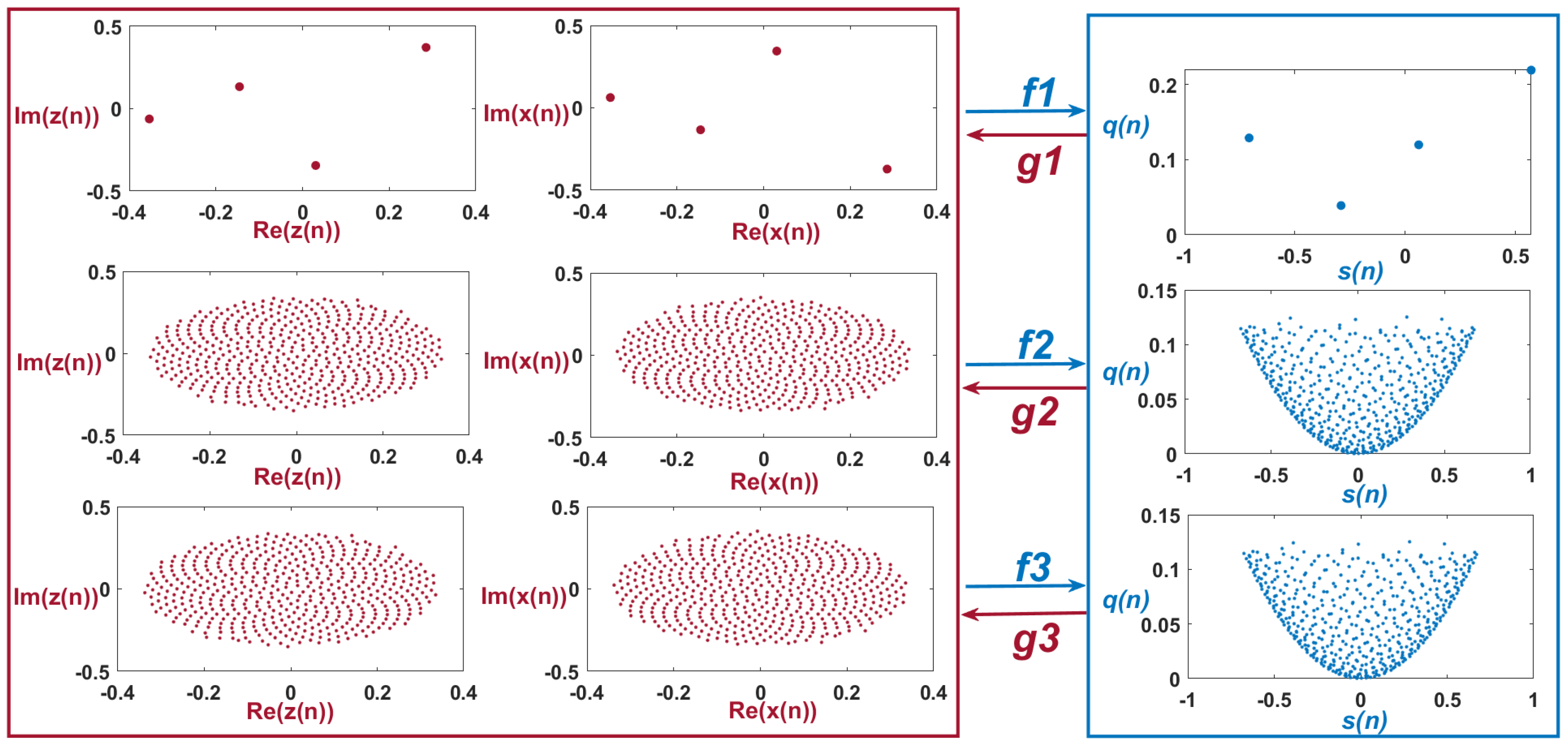
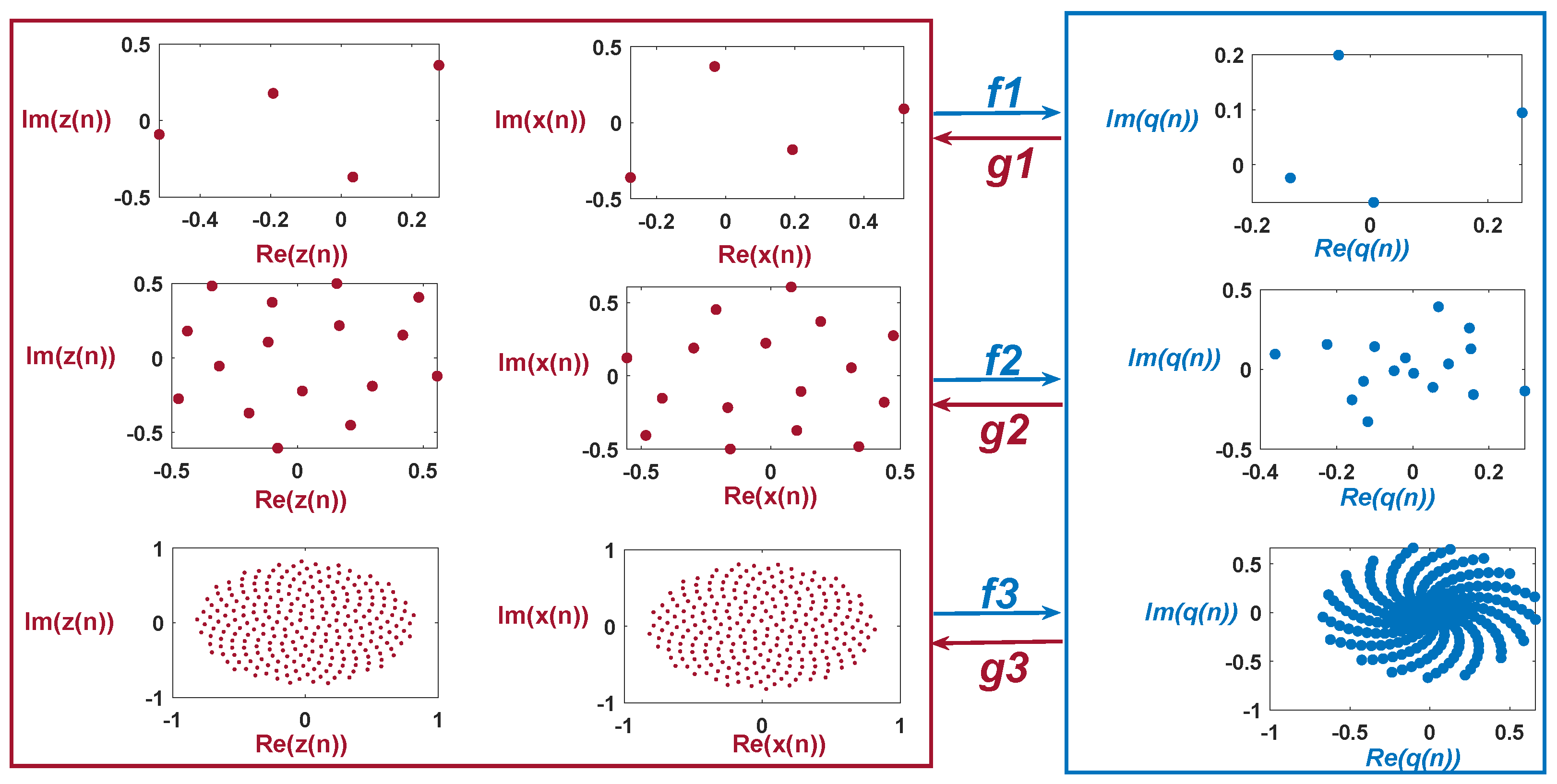
3. GAM on the Symmetrized Bidisc

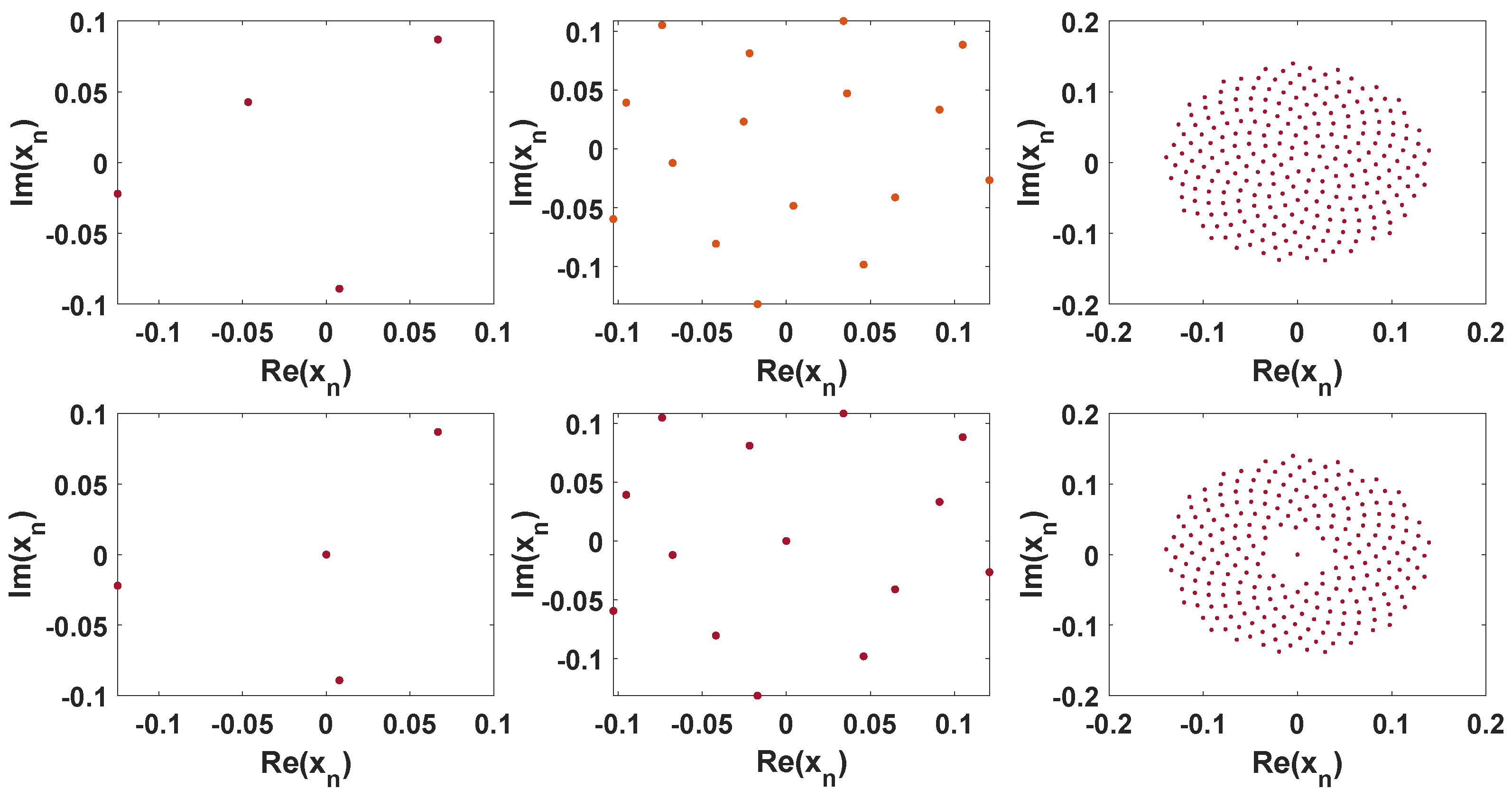
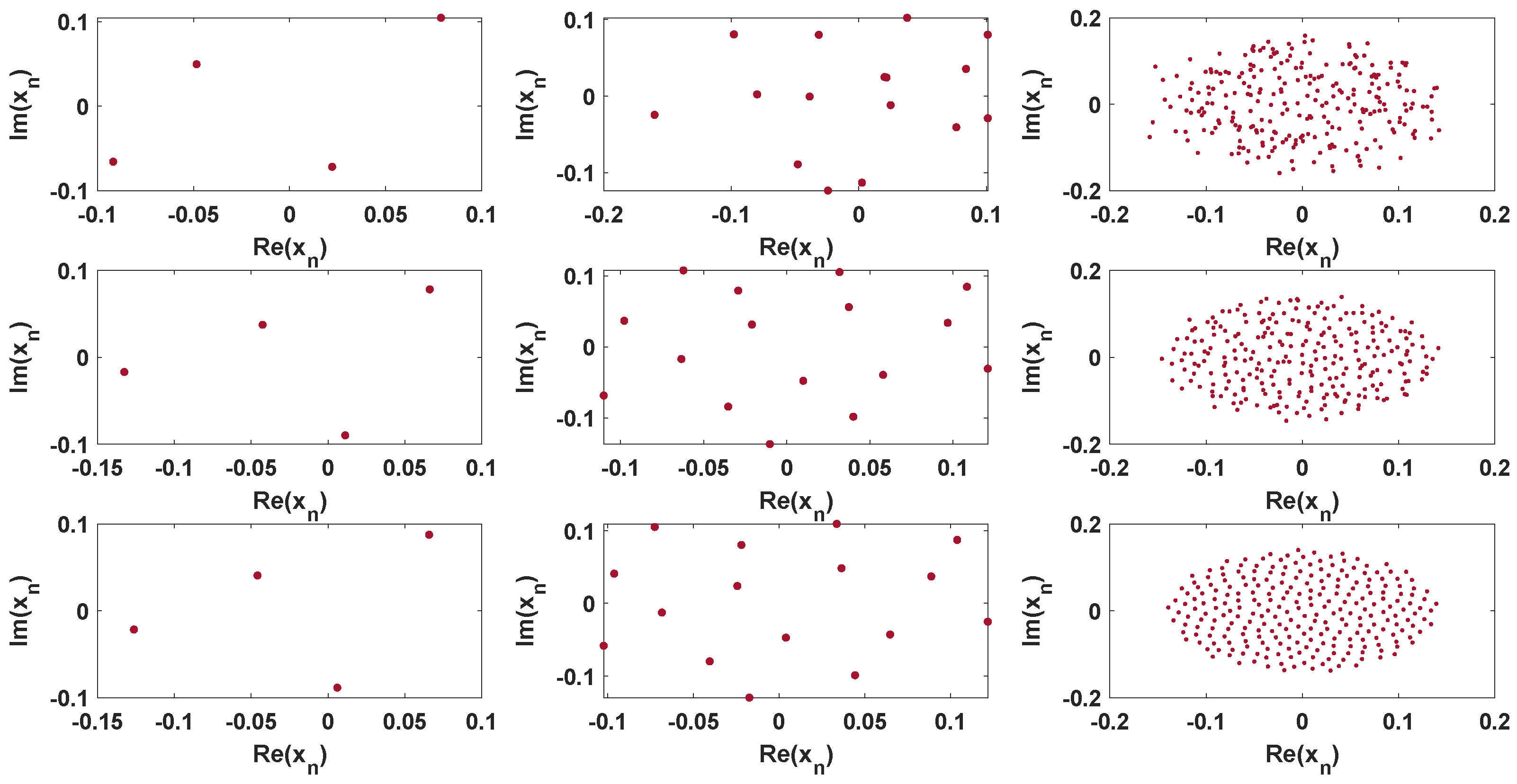
3.1. Bd-GAM1

With the definition of ${\mathbb{G}}_2$, the Bd-GAM1 can be modeled as

$$\begin{array}{c}\hfill (x_n,z_n)\stackrel{f}{\to }(x_n+z_n,x_n{z}_n)\iff (z_n,\overline{z_n})\stackrel{f}{\to }(2Re\left(z_n\right),{\left|z_n\right|}^2)\iff (Re\left(z_n\right),r_n^2),\end{array}$$

(18)

where $x_n=\overline{z_n}$. Denote $(s_n,q_n)=(Re\left(z_n\right),{\left|z_n\right|}^2)$, $r_n=c_{disc}\sqrt{n},z_n=r_n{e}^{i2\pi \theta n},n\in \{1,2,\dots ,N\}$ and $Re\left(z_n\right)=r_{n}cos\left(2\pi \theta n\right)$. As the average power of constellation points is a constraint, there is

$$\begin{array}{cc}\hfill \tilde{P}& =\sum _{n=1}^N(2p_n-p_n^2)s_n^2+\sum _{n=1}^N{p}_n^2{q}_n^2\hfill \\ \hfill & =\sum _{n=1}^N(2p_n-p_n^2){(x_n+z_n)}^2+\sum _{n=1}^N{p}_n^2{\left(x_n{z}_n\right)}^2\hfill \\ \hfill & ={\displaystyle \frac{\left({\sum }_{n=1}^N{n}^2\right){\left(c_{disc}^2\right)}^2}{N^2}}+{\displaystyle \frac{c_{disc}^2({\sum }_{n=1}^{N}co{s}^2\left(2\pi \theta n\right)·n)(2N-1)}{N^2}}\hfill \\ \hfill & =c1·{\left(c_{disc}^2\right)}^2+c2·\left(c_{disc}^2\right)\hfill \\ \hfill & \Rightarrow c_{disc}=\sqrt{{\displaystyle \frac{-c2+\sqrt{{\left(c2\right)}^2+4·c1·\tilde{P}}}{2c1}}}(c_{disc}>0),\hfill \end{array}$$

(19)

where $\mathrm{c}1={\displaystyle \frac{{\sum }_{n=1}^N{n}^2}{N^2}}={\displaystyle \frac{{\pi }^2}{6N^2}}$. $\mathrm{c}2$ is bounded as the number of constellation points N are not infinite. In fact, ${\sum }_{n=1}^{N}co{s}^2\left(2\pi \theta n\right)·n={\sum }_{n=1}^N{\displaystyle \frac{cos\left(4\pi \theta n\right)·n}{2}}+{\displaystyle \frac{N(N+1)}{4}}$. The series ${\sum }_{n=1}^N{\displaystyle \frac{cos\left(4\pi \theta n\right)·n}{2}}$ is bounded as N is not infinite. The boundary is shown in Figure 4. The upper bound and lower bound are often a good constraint of c2.

Figure 4. The Upper/Lower bound for choosing the sum of series ${\sum }_{n=1}^{N}co{s}^2\left(2\pi \theta n\right)·n$.

As $c_{disc}$ is bounded, this makes the Bd-GAM possible with higher dimensions. Compared with $c_{disc}$ in [12,13,14], Bd-GAM1 can alter the value based on the complex variable $z_n$ and the number of points. Meanwhile, the amplitude is $r_n\propto \sqrt{n}$. As $r_n$ depends on $z_n$ and N, the following MI optimization problem can be solved without the limitation of constellation size.

Figure 5 shows the normalized Bd-GAM1 signal constellation with different points. The left part (red box) of this figure is the original image set, denoted by ${\mathbb{D}}^2=\{(z_n,x_n)\in {\mathbb{C}}^2:|z_n|<1,|x_n|<1\}$. The right region (blue box) is the image set $\left\{(x_n+z_n,x_n{z}_n)\right\}$ under ${\left\{f_j\right\}}_{j=1}^3(f_j=(f_{j1},f_{j2}),f_{jk}:\mathbb{D}\mapsto {\mathbb{G}}_2)$. The In-phase and Quadrature of signal are $s_n$ and $q_n$. Then we have $(s_n,q_n)=(Re\left(z_n\right),r_n^2)\iff (x_n+z_n,x_n{z}_n)$, where $(Re\left(z_n\right),r_n^2)\in {\mathbb{R}}^2$. ${\left\{g_j\right\}}_{j=1}^3(g_j=(g_{j1},g_{j2}))$ is the inverse mapping set. Note that it is the discretized bell shaping, with the large probability values at the bottom of bell. The design is naturally sparse in nature leading to a lowering of shaping-loss.

Figure 5. Normalized Bd-GAM1 signal constellation with $N\in \{2^2,2^4,2^8\}$.

Disc-GAM [12] has better PAPR performance than QAM, while QAM has 1.53 dB SNR-gap to the AWGN Shannon capacity [3]. Here, PSK has ${\mathrm{PAPR}}_{\mathrm{PSK}}=0$ dB with poor MI-performance. In Table 1, we present in a unified way entropy and PAPR of five different modulation methods. The entropy and PAPR of Bd-GAM1 in ${\mathbb{C}}^2$ are ${log}_{2}2N$ and ${\displaystyle \frac{2N}{2N+1}}\simeq 1$ dB ($N\to \infty$). The power normalization of original constellation point is $2N+1$. Compared to 2 dB for Disc-GAM on $\mathbb{D}$, the peak-to-average SNR Ratio is 1 dB for Bd-GAM1 on ${\mathbb{G}}_2$. Thus, Bd-GAM1 has a noticeable gap to the Disc-GAM.

Table 1. Entropy and PAPR values for different modulation methods ¹.

Modulation Format	Entropy	PAPR ($\mathit{N}\to \mathit{\infty }$)
Bd-GAM1 prop.	$H_1={log}_{2}2N$	${\mathrm{PAPR}}_1={\displaystyle \frac{2N}{2N+1}}$ dB ≃ 1 dB
Bd-GAM2 prop.	$H_2={log}_{2}2N$	${\mathrm{PAPR}}_2$ = ${\mathrm{PAPR}}_1$
Disc-GAM [12]	$H_3={log}_{2}N$	${\mathrm{PAPR}}_3={\displaystyle \frac{2N}{N+1}}\simeq 2$ dB
Geometric-bell-GAM [12]	$H_4={log}_{2}N$	${\mathrm{PAPR}}_4={\displaystyle \frac{\tilde{P}}{1-ln\frac{(n!)}{NlnN}}}\simeq \tilde{P}ln\left(N\right)$
Generalized Disc-GAM [14]	$H_5={log}_2{\displaystyle \frac{2\tilde{P}N{N}_s}{N_s(N_s+1)-N_o(N_o-1)}}$	${\mathrm{PAPR}}_5\simeq$ 2 dB

¹ As $N\to \infty$, the average power and peak power of QAM is higher than Disc-GAM with same average constellation point distances.

3.2. Bd-GAM2

Bd-GAM2 is characterized by

$$\begin{array}{c}\hfill (x_n,z_n)\stackrel{f}{\to }(x_n+z_n,x_n{z}_n)\iff (z_n,-z_n)\stackrel{f}{\to }(0,-z_n{z}_n)\iff (0,-r_n^2{e}^{i4\pi \theta n}),\end{array}$$

(20)

where $x_n=-z_n$. Denote $(s_n,q_n)=(0,-r_n^2{e}^{i4\pi \theta n}),r_n=c_{disc}\sqrt{n},z_n=r_n{e}^{i2\pi \theta n},n\in \{1,2,\cdots ,N\}$. The average power of constellation points is

$$\begin{array}{cc}\hfill \tilde{P}& =\sum _{n=1}^N{p}_n^2{\left(x_n{z}_n\right)}^2=\sum _{n=1}^N{p}_n^2{q}_n^2=\sum _{n=1}^N{\displaystyle \frac{1}{N^2}}{r}_n^4{e}^{i8\pi \theta n}\hfill \\ \hfill & \Rightarrow c_{disc}=\sqrt[4]{{\displaystyle \frac{N^2}{\left({\sum }_{n=1}^N{n}^2{e}^{i8\pi \theta n}\right)}}}(c_{disc}>0)\hfill \end{array}$$

(21)

Set $N\in \{2^2,2^4,2^8\}$. The corresponding constellation of Bd-GAM2 is Figure 6. The left part (red box) of this figure is the original image set, denoted by ${\mathbb{D}}^2=\{(z_n,x_n)\in {\mathbb{C}}^2:|z_n|<1,|x_n|<1\}$. The right region (blue box) is the image set $\left\{(x_n+z_n,x_n{z}_n)\right\}$ under ${\left\{f_j\right\}}_{j=1}^3(f_j=(f_{j1},f_{j2}),f_{jk}:\mathbb{D}\mapsto {\mathbb{G}}_2)$. Then we have $(s_n,q_n)=(0,-r_n^2{e}^{i4\pi \theta n})\iff (x_n+z_n,x_n{z}_n)$. ${\left\{g_j\right\}}_{j=1}^3(g_j=(g_{j1},g_{j2}))$ is the inverse mapping set. If N is large, the signal constellation can offer a good distribution of energy due to MI performance of probabilistic Bd-GAM2. Note that, when $N\to \infty$, PAPR ≃ 1 dB in Table 1. The circular design can offer enhanced MI performance over Disc-GAM and square-QAM design.

Figure 6. Normalized Bd-GAM2 signal constellation with $N\in \{2^2,2^4,2^8\}$.

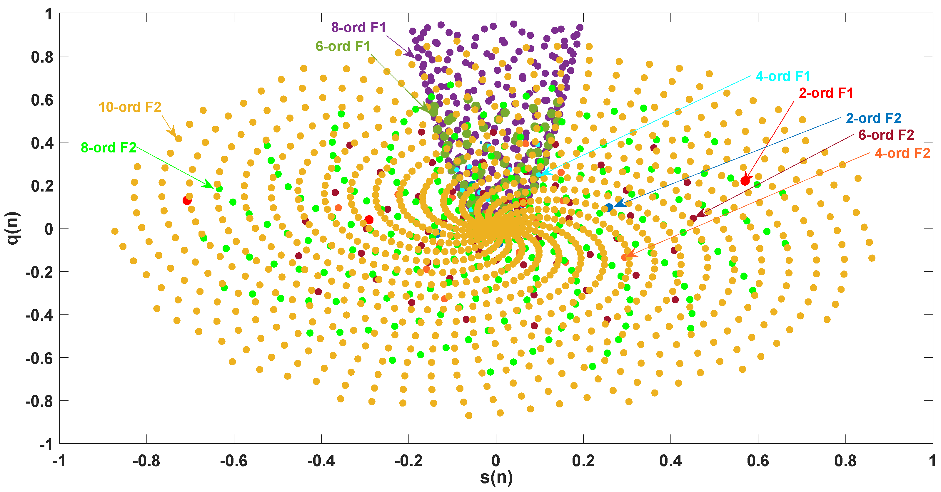
3.3. The Complex Geometric Properties Analysis of Bd-GAM1/2

In this part, we present the Bd-GAM signal constellation in Figure 7. Each modulation signal points of Bd-GAM are labeled with the same color as their labels (i.e., n-ord F1/F2 stand for Bd-GAM1/2 with $N=2^n$). We note that the shapes of Bd-GAM2 constellation expand as the modulations increase from 2 to 10. Compared with Bd-GAM2, the geometric shaping of Bd-GAM1 is symmetric and the boundary points shrink toward the center as the modulation N increases. The inner points fill the interior of the bell along the direction of the tangent vector. In contrast to GAM, with natural constellation point indexing, the proposed Bd-GAM can provide enhanced distance performance. In the following, we plot the orbit for the points of the Bd-GAM signal constellation.

Figure 7. Bd-GAM1/2 signal constellation aggregation.

Figure 8 plots the orbit for each modulation signal. The left part of this figure is the orbit for the symmetric center of Bd-GAM1. The orbit of the constellatio points becomes more flattened as the radius increases. Meanwhile, the orbit for the boundary points of Bd-GAM2 expands with spiral phyllotaxis packing.

Figure 8. Orbit for the points of Bd-GAM1/2.

3.4. MI Optimization Problem of Probabilistic- and Geometric- Bd-GAM: Bd-GAM1/2

Let N be the number of constellation points. $p_n={\displaystyle \frac{1}{N}}$ is the probability for each constellation point. Similar to $G1$ method [12], Bd-GAM1/2 can control the radius $r_n$ to maximize the MI. It is a difference that the proposed methods can synchronously select the radius and phase by optimizing just a variable $z_n$. With this method, we optimize $z_n$ that maximizes the MI for a given SNR. In the region $(s_n,q_n)$, the optimized n-th signal constellation point is $z_n^{*}=r_n^{*}{e}^{i2\pi \theta n}$. Denote the complex valued output $\mathit{y}(\mathit{y}=\mathit{r}{e}^{i{\vartheta }_k})$ by r.v. Y. The complex valued input with discrete modulation is r.v. Z. Then we have the following MI-optimization problem

$$\begin{array}{cc}\hfill & \underset{z_n}{maximize}I(Y,Z)\hfill \\ \hfill & s.t.|z_{n+1}|>|z_n|,|z_1|\ge 0,\hfill \\ \hfill & \sum _{n=1}^N{\displaystyle \frac{p_n{\left|z_n\right|}^2}{{\sigma }^2}}=S,\sum _{n=1}^N{p}_n=1,n=\{1,2,\cdots ,N\}.\hfill \end{array}$$

(22)

In the above, the mutual information I can be expressed with terms i.e., the differential entropy $h\left(Y\right)$ and conditional differential entropy $h\left(Y\right|Z)$. Meanwhile, we have $I\left(Y\right|Z)=h(Y)-h(Y\left|Z\right)=h\left(Y\right)-h\left(W\right)$, where $h\left(W\right)={log}_2\left(\pi e{\sigma }^2\right),h\left(Y\right)=-{\int }_{\mathbb{C}}{f}_Y{log}_2\left(f_Y\right)dy$. $h\left(Y\right)$ integrates in the complex domain and

$$\begin{array}{c}\hfill f_Y=\sum _{n=1}^{N}f\left(\mathit{y}\right|z_n)p_n={\displaystyle \frac{1}{\pi {\sigma }^2}}\sum _{n=1}^N{p}_n{e}^{-{\displaystyle \frac{{(\mathit{y}-z_n)}^2}{{\sigma }^2}}}.\end{array}$$

(23)

As for the densest point at the center, i.e., where the pdf for the complex Gaussian r.v. peaks, it is a peak point relative to ${\mathbb{G}}_2$ if there is a holomorphic funtion f satisfying $f\left(\xi \right)=1$ and $\left|f\right(\xi \left)\right|<1$ for all $\xi \in \overline{{\mathbb{G}}_2}\setminus \left\{\xi \right\}$. Thus, it needs to prove that the region of the signal constellation points is a pseudoconvex domain. Then we can find some function to design the radius in the region. Equation (23) is hard to solve. We can get the discrete formation of $h\left(Y\right)$ as follows

$$\begin{array}{cc}\hfill & I(Y,Z)\hfill \\ \hfill & =-{\int }_{\mathbb{C}}{\displaystyle \frac{1}{\pi {\sigma }^2}}\sum _{n=1}^N{p}_n{e}^{{\displaystyle \frac{-{(\mathit{y}-z_n)}^2}{{\sigma }^2}}}({log}_2({\displaystyle \frac{1}{\pi {\sigma }^2}})+{log}_2(\sum _{n=1}^N{p}_n{e}^{{\displaystyle \frac{-{(\mathit{y}-z_n)}^2}{{\sigma }^2}}}))dy\hfill \\ \hfill & =\sum _K\{{\displaystyle \frac{S}{\pi ({\sum }_{n=1}^N|z_n{|}^2)}}\sum _{n=1}^N{e}^{{\displaystyle \frac{-NS{({\mathit{y}}^{(k)}-z_n)}^2}{{\sum }_{n=1}^N{\left|z_n\right|}^2}}}({log}_2({\displaystyle \frac{NS}{\pi ({\sum }_{n=1}^N|z_n{|}^2)}})+\hfill \\ \hfill & {log}_2(\sum _{n=1}^N{\displaystyle \frac{1}{N}}{e}^{{\displaystyle \frac{-NS{({\mathit{y}}^{(k)}-z_n)}^2}{{\sum }_{n=1}^N{\left|z_n\right|}^2}}}))\}d\mathit{y}(k=\{1,2,\cdots ,K\}).\hfill \end{array}$$

(24)

In Equation (24), we put $C_1(|z_n|):={\displaystyle \frac{S}{\pi ({\sum }_{n=1}^N|z_n{|}^2)}}$, $C_2(|z_n|):={log}_2({\displaystyle \frac{NS}{\pi ({\sum }_{n=1}^N|z_n{|}^2)}})$, the sum of the series ${\sum }_{n=1}^N{e}^{{\displaystyle \frac{-NS{({\mathit{y}}^{(k)}-z_n)}^2}{{\sum }_{n=1}^N{\left|z_n\right|}^2}}}:=T_1^k(z_n)$ and ${\sum }_{n=1}^N{\displaystyle \frac{1}{N}}{e}^{{\displaystyle \frac{-NS{({\mathit{y}}^{(k)}-z_n)}^2}{{\sum }_{n=1}^N{\left|z_n\right|}^2}}}:=T_2^k(z_n)$. Then we have

$$\begin{array}{cc}\hfill & I(Y,Z)=\hfill \\ \hfill & \{2\{C_1{C}_2\sum _{k=2}^{K-1}{T}_1^K+C_1\sum _{k=2}^{K-1}{T}_1^k{log}_2(T_2^k)\}+\{C_1{C}_2{T}_1^1+C_1{T}_1^1+C_1{T}_1^1{log}_2(T_2^1)\}\hfill \\ \hfill & +\{C_1{C}_2{T}_1^K+C_1{T}_1^K{log}_2(T_2^K)\}\}{\displaystyle \frac{(-sin{\vartheta }_k+icos{\vartheta }_k){\mathit{r}}_k{\sum }_K{\vartheta }_k}{2N}}.\hfill \end{array}$$

(25)

For $\xi =(Y,Z)$ and $t=\{t_1,t_2\}$, we can write $L_{\xi }(I,t)$ for ${\sum }_{n,m=1}^2{\displaystyle \frac{{\partial }^{2}I}{\partial z_n\partial \overline{z_m}}}$$(\xi )t_j\overline{t_k}$. The baseband samples are ${\mathit{y}}^{(k)}={\mathit{z}}^{(k)}+{\mathit{w}}^{(k)}$. The bivariate conditional pdf is $p(\mathit{y}|\mathit{z})={\displaystyle \frac{{-|\mathit{y}-\mathit{z}|}^2}{{\sigma }^2}}$. Without loss of generality, we let tangent vector $t=(-I_{z_n},I_{\mathit{y}})\in T_{\xi }^C(\partial \Omega )=\{t\in {\mathbb{C}}^2:\partial I_{\xi }(t)=0\}$ and boundary point $\xi \in \partial {\mathbb{G}}_2\setminus \{0\}$ here. Calculations lead to the following formula:

$$\begin{array}{cc}\hfill & {\displaystyle \frac{\partial I(\xi )}{\partial z_n}}={\displaystyle \frac{1}{N\pi {\sigma }^{4}ln2}}{\int }_{\mathbb{C}}{e}^{{\displaystyle \frac{-{(\mathit{y}-z_n)}^2}{{\sigma }^2}}}\overline{z_n}(1+ln(f_Y))d\mathit{y}\hfill \\ \hfill & {\displaystyle \frac{\partial I(\xi )}{\partial \overline{z_n}}}={\displaystyle \frac{1}{N\pi {\sigma }^{4}ln2}}{\int }_{\mathbb{C}}{e}^{{\displaystyle \frac{-{(\mathit{y}-z_n)}^2}{{\sigma }^2}}}(z_n-2Re(\mathit{y}))(1+ln(f_Y))d\mathit{y}\hfill \\ \hfill & {\displaystyle \frac{{\partial }^{2}I(\xi )}{\partial z_n\partial \overline{z_n}}}={\displaystyle \frac{1}{N\pi {\sigma }^{4}ln2}}{\int }_{\mathbb{C}}{e}^{{\displaystyle \frac{-{(\mathit{y}-z_n)}^2}{{\sigma }^2}}}\{(1+ln(f_Y))(\overline{z_n}-{\displaystyle \frac{z_n-2Re(\mathit{y})}{{\sigma }^2}})-{\displaystyle \frac{\overline{z_n}(z_n-2Re(\mathit{y}))}{{\sigma }^2}}\}d\mathit{y}.\hfill \end{array}$$

(26)

Similarly, we have

$$\begin{array}{cc}\hfill & {\displaystyle \frac{\partial I(\xi )}{\partial \mathit{y}}}={\displaystyle \frac{1}{\pi {\sigma }^2}}\sum _{n=1}^N{p}_n{e}^{{\displaystyle \frac{-{(\mathit{y}-z_n)}^2}{{\sigma }^2}}}({log}_2({\displaystyle \frac{1}{\pi {\sigma }^2}})+{log}_2(\sum _{n=1}^N{p}_n{e}^{{\displaystyle \frac{-{(\mathit{y}-z_n)}^2}{{\sigma }^2}}}))\hfill \\ \hfill & {\displaystyle \frac{\partial I(\xi )}{\partial \overline{\mathit{y}}}}=({\displaystyle \frac{{log}_2\frac{1}{\pi {\sigma }^2}}{N\pi {\sigma }^4}}-{log}_2{\displaystyle \frac{e^{\frac{-{(\mathit{y}-z_n)}^2}{{\sigma }^2}}}{N}}-{\displaystyle \frac{ln2}{{\sigma }^2}}){\int }_{\mathbb{C}}\sum _{n=1}^N(\mathit{y}-z_n)e^{{\displaystyle \frac{-{(\mathit{y}-z_n)}^2}{{\sigma }^2}}}d\mathit{y}\hfill \\ \hfill & {\displaystyle \frac{{\partial }^{2}I(\xi )}{\partial \overline{\mathit{y}}\partial z_n}}={\int }_C({\displaystyle \frac{z_n(\mathit{y}-z_n)}{{\sigma }^2}})e^{{\displaystyle \frac{-(\mathit{y}-z_n)}{{\sigma }^2}}}d\mathit{y}\hfill \\ \hfill & {\displaystyle \frac{{\partial }^{2}I(\xi )}{\partial \mathit{y}\partial \overline{z_n}}}={\displaystyle \frac{e^{\frac{-{(\mathit{y}-z_n)}^2}{{\sigma }^2}}}{N\pi {\sigma }^{4}ln2}}\{(1+ln(f_Y))(\overline{{\mathit{z}}_{\mathit{n}}}-{\displaystyle \frac{z_n-2Re(\mathit{y})}{{\sigma }^2}})-{\displaystyle \frac{\overline{z_n}(z_n-2Re(\mathit{y}))}{{\sigma }^2}}\}\hfill \\ \hfill & {\displaystyle \frac{{\partial }^{2}I(\xi )}{\partial \mathit{y}\partial \overline{\mathit{y}}}}={\displaystyle \frac{e^{\frac{-{(\mathit{y}-z_n)}^2}{{\sigma }^2}}}{N\pi {\sigma }^{4}ln2}}\{(1+ln(f_Y))(\overline{\mathit{y}}-{\displaystyle \frac{\mathit{y}-2Re(z_n)}{{\sigma }^2}})-{\displaystyle \frac{\overline{\mathit{y}}(\mathit{y}-2Re({\mathit{z}}_{\mathit{n}}))}{{\sigma }^2}}\}.\hfill \end{array}$$

(27)

Let the average power of the signal be normalized and the noise variance is ${\sigma }^2={\displaystyle \frac{1}{S}}$. We also have the discrete formation. It follows that

$$\begin{array}{cc}\hfill & {\displaystyle \frac{\partial T_1^k}{\partial z_n}}=({\displaystyle \frac{-NS}{{\sum }_n^N{\left|z_n\right|}^2}})e^{{\displaystyle \frac{-NS{({\mathit{y}}^{(k)}-z_n)}^2}{{\sum }_{n=1}^N{\left|z_n\right|}^2}}}\overline{z_n},{\displaystyle \frac{\partial T_2^k}{\partial z_n}}={\displaystyle \frac{1}{N}}({\displaystyle \frac{\partial T_1^k}{\partial z_n}})\hfill \\ \hfill & {\displaystyle \frac{\partial T_1^k}{\partial \overline{z_n}}}=({\displaystyle \frac{-NS}{{\sum }_{n=1}^N{\left|z_n\right|}^2}})e^{{\displaystyle \frac{-NS{({\mathit{y}}^{(k)}-z_n)}^2}{{\sum }_{n=1}^N{\left|z_n\right|}^2}}}(z_n-2Re(\mathit{y})),{\displaystyle \frac{\partial T_2^k}{\partial \overline{z_n}}}={\displaystyle \frac{1}{N}}({\displaystyle \frac{\partial T_1^k}{\partial \overline{z_n}}})\hfill \\ \hfill & {\displaystyle \frac{\partial T_1^k}{\partial \mathit{y}}}=({\displaystyle \frac{-2NS}{{\sum }_n^N{\left|z_n\right|}^2}})e^{{\displaystyle \frac{-NS{({\mathit{y}}^{(k)}-z_n)}^2}{{\sum }_{n=1}^N{\left|z_n\right|}^2}}}({\mathit{y}}^{(k)}-z_n),{\displaystyle \frac{\partial T_2^k}{\partial \mathit{y}}}={\displaystyle \frac{1}{N}}{\displaystyle \frac{\partial T_1^k}{\partial \mathit{y}}}\hfill \\ \hfill & {\displaystyle \frac{\partial T_1^k}{\partial \overline{\mathit{y}}}}=({\displaystyle \frac{-2NS}{{\sum }_n^N{\left|z_n\right|}^2}})e^{{\displaystyle \frac{-NS{({\mathit{y}}^{(k)}-z_n)}^2}{{\sum }_{n=1}^N{\left|z_n\right|}^2}}}(\overline{{\mathit{y}}^{(k)}}-\overline{z_n}),{\displaystyle \frac{\partial T_2^k}{\partial \overline{\mathit{y}}}}={\displaystyle \frac{1}{N}}{\displaystyle \frac{\partial T_1^k}{\partial \mathit{y}}}.\hfill \end{array}$$

$$\begin{array}{cc}\hfill & {\displaystyle \frac{{\partial }^2{T}_1^k}{\partial z_n\partial \overline{z_n}}}=({\displaystyle \frac{NS}{{\sum }_{n=1}^N{\left|z_n\right|}^2}})e^{{\displaystyle \frac{-NS{({\mathit{y}}^{(k)}-z_n)}^2}{{\sum }_{n=1}^N{\left|z_n\right|}^2}}}({\displaystyle \frac{NS\overline{z_n}}{{\sum }_{n=1}^N{\left|z_n\right|}^2}}(z_n-2Re(\mathit{y}))-1)\hfill \\ \hfill & {\displaystyle \frac{{\partial }^2{T}_2^k}{\partial z_n\partial \overline{z_n}}}={\displaystyle \frac{1}{N}}{\displaystyle \frac{{\partial }^2{T}_1^k}{\partial z_n\partial \overline{z_n}}}\hfill \\ \hfill & {\displaystyle \frac{{\partial }^2\{T_1^k{log}_2(T_2^k)\}}{\partial z_n\partial \overline{z_n}}}=({log}_2(T_2^k)+{\displaystyle \frac{T_1^k{T}_2^k-T_1^k+2T_2^k}{N{(T_2^k)}^2}}ln2){\displaystyle \frac{{\partial }^2{T}_1^k}{\partial z_n\partial \overline{z_n}}}\hfill \\ \hfill & {\displaystyle \frac{{\partial }^{2}I(Y,Z)}{\partial z_n\partial \overline{z_n}}}=\hfill \\ \hfill & \{2\{C_1{C}_2\sum _{k=1}^{K-1}{\displaystyle \frac{{\partial }^2{T}_1^k}{\partial z_n\partial \overline{z_n}}}+C_1\sum _{k=1}^{K-1}{\displaystyle \frac{{\partial }^2\{T_1^k{log}_2(T_2^k)\}}{\partial z_n\partial \overline{z_n}}}\}+\{C_1{C}_2{\displaystyle \frac{{\partial }^2{T}_1^1}{\partial z_n\partial \overline{z_n}}}+C_1\hfill \\ \hfill & {\displaystyle \frac{{\partial }^2\{T_1^1{log}_2(T_2^1)\}}{\partial z_n\partial \overline{z_n}}}\}+\{C_1{C}_2{\displaystyle \frac{{\partial }^2{T}_1^K}{\partial z_n\partial \overline{z_n}}}+C_1{\displaystyle \frac{{\partial }^2\{T_1^K{log}_2(T_2^K)}{\partial z_n\overline{\partial }{z}_n}}\}\}(-sin{\vartheta }_k+\hfill \\ \hfill & icos{\vartheta }_k){\mathit{r}}_k\sum _K{\vartheta }_{k}2N.\hfill \end{array}$$

(28)

For the output Y, the Levi form is

$$\begin{array}{c}\hfill L_{\xi }(I,t)=I_{Y\overline{Y}}|I_Z{|}^2-I_{Y\overline{Z}}{I}_Z{I}_{\overline{Y}}-I_{\overline{Y}Z}{I}_{\overline{Z}}{I}_{\overline{Y}}+I_{Z\overline{Z}}{\left|I_Y\right|}^2.\end{array}$$

(29)

By Equations (25) and (28), semi-positive definiteness of Equation (29) can be verfied. It proves that the complex domain defined by function $f_Y$ is a pseudoconvex domain. We can find a local system of holomorphic coordinates to get the signal constellations.

4. Numerical Results and Discussions

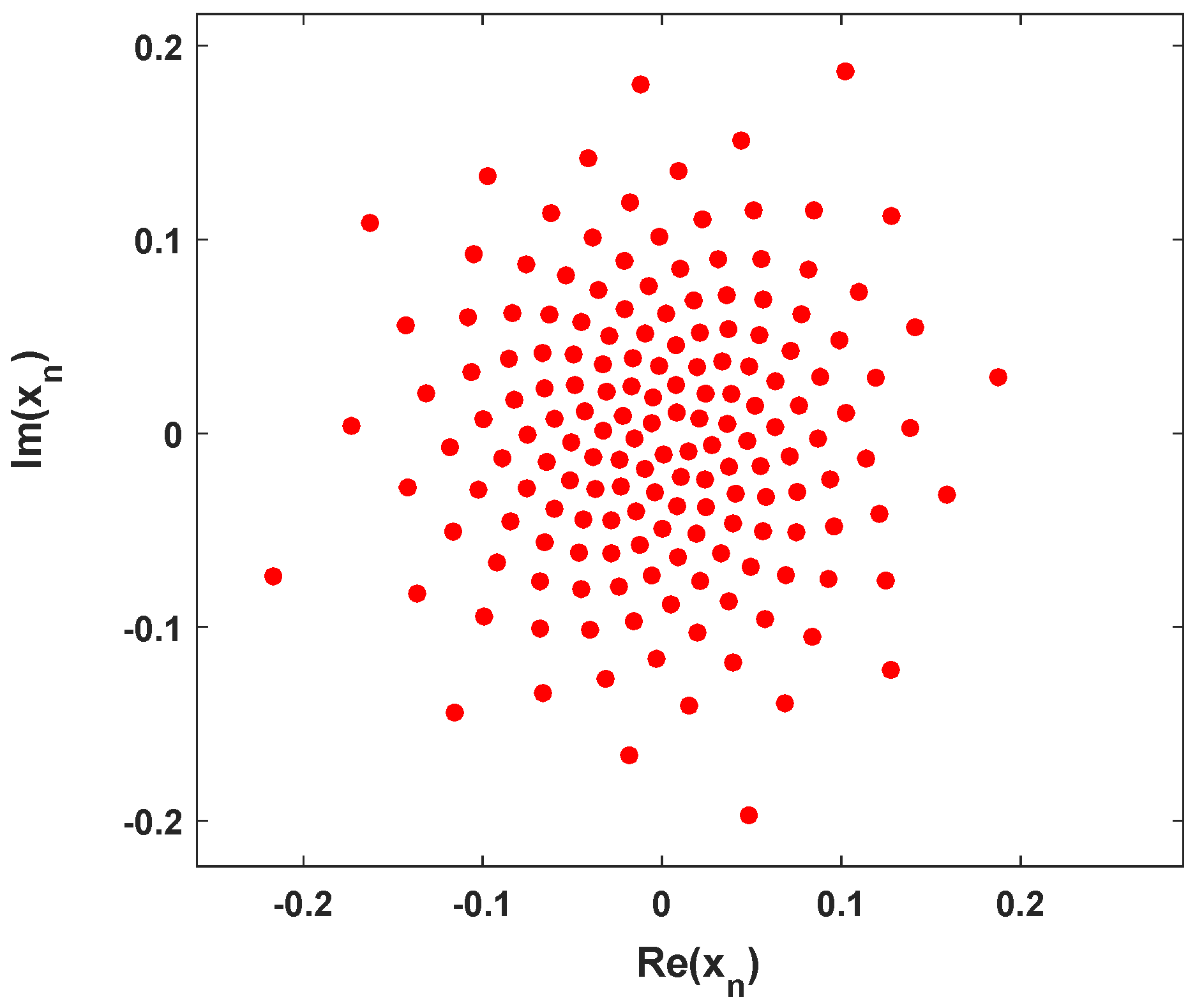
4.1. Magnitude Distribution of Bd-GAM1

In Figure 9, we plot the magnitude distribution of Bd-GAM1 with different constellation points (i.e., $N\in \{2^2,2^4,2^8\}$). Without noise, the first column of this figure presents the magnitude distribution for constellation points of Bd-GAM1 in ${\mathbb{C}}^2$ (denoted as ${\mathrm{C}}_{\mathrm{G}2}$) and points of Disc-GAM [12] in $\mathbb{C}$ (denoted as d). We observe that the signal constellation magnitudes of Bd-GAM1 are larger than magnitudes of Disc-GAM. The middle column of it is the magnitude distribution with SNR = 22.5 dB. For the $c_{disc}$ of Bd-GAM1, it approximates the function of Equation (19) with some oscillaroy behavior. In the eighth subplot, we can see that there exist some little oscillatory problem for the initial constellation points. The last column contains three subplots of magnitude distribution for constellation points in ${\mathbb{G}}_2$. Let ‘${\mathrm{K}}_{\mathrm{G}2}^{*}$’ stand for the Bd-GAM1 with SNR = 22.5dB and ‘${\mathrm{K}}_{\mathrm{G}2}$’ is the case without noise. The signal constellation magnitudes of ‘${\mathrm{K}}_{\mathrm{G}2}^{*}$’ have the same distribution as the ‘${\mathrm{K}}_{\mathrm{G}2}$’. Clearly, we can see that Bd-GAM1 has a stable magnitude distribution and good ability to overcome the noise.

Figure 9. Magnitude distribution of Bd-GAM1 with different constellation points ($N\in \{2^2,2^4,2^8\}$).

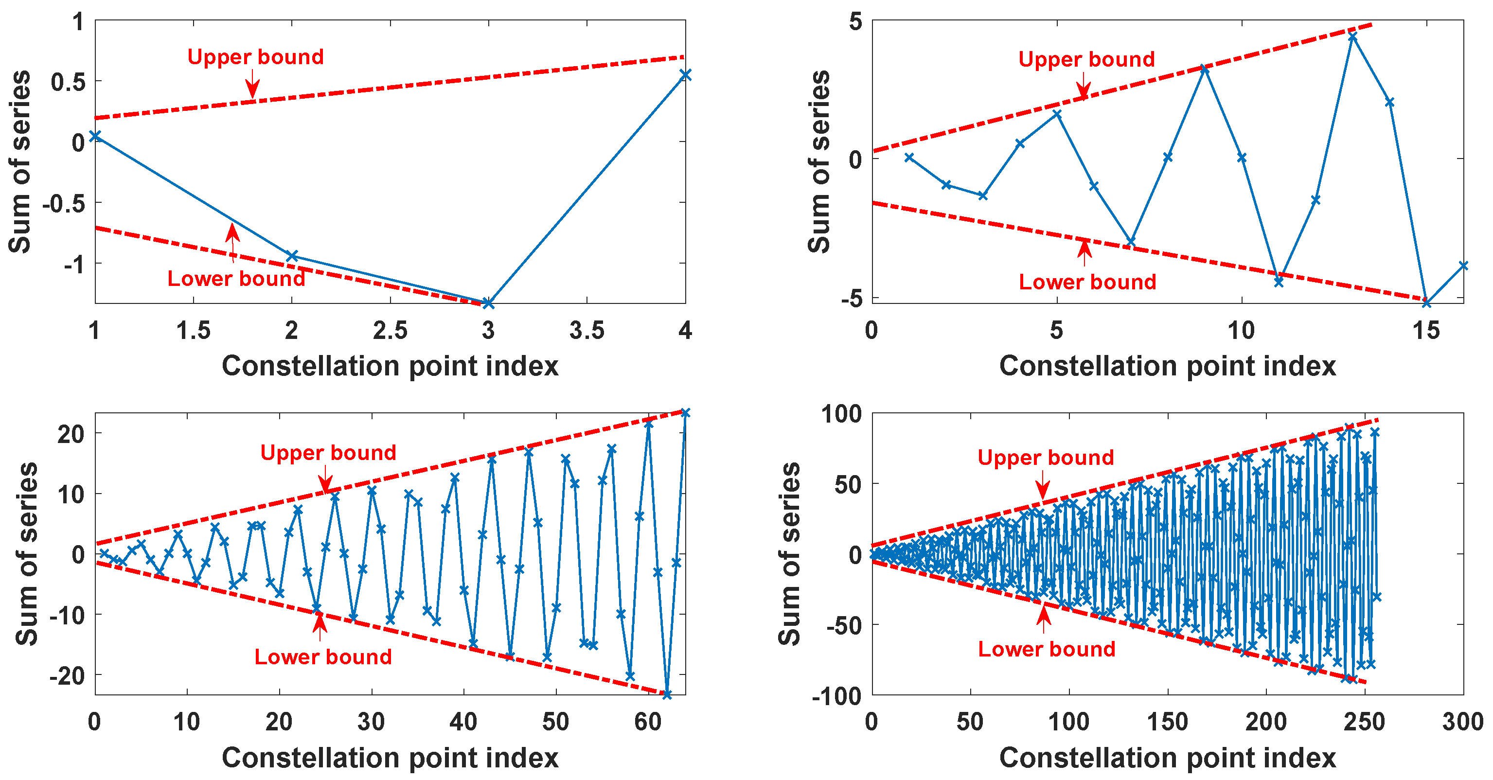
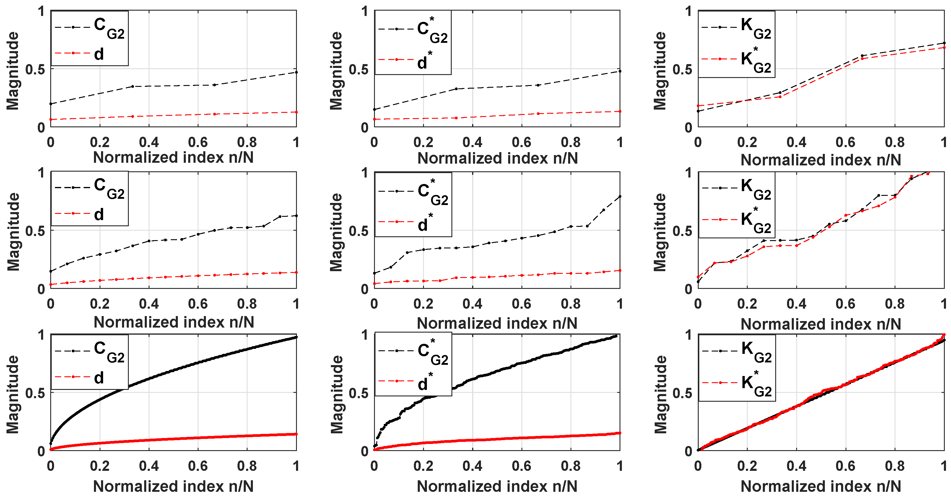
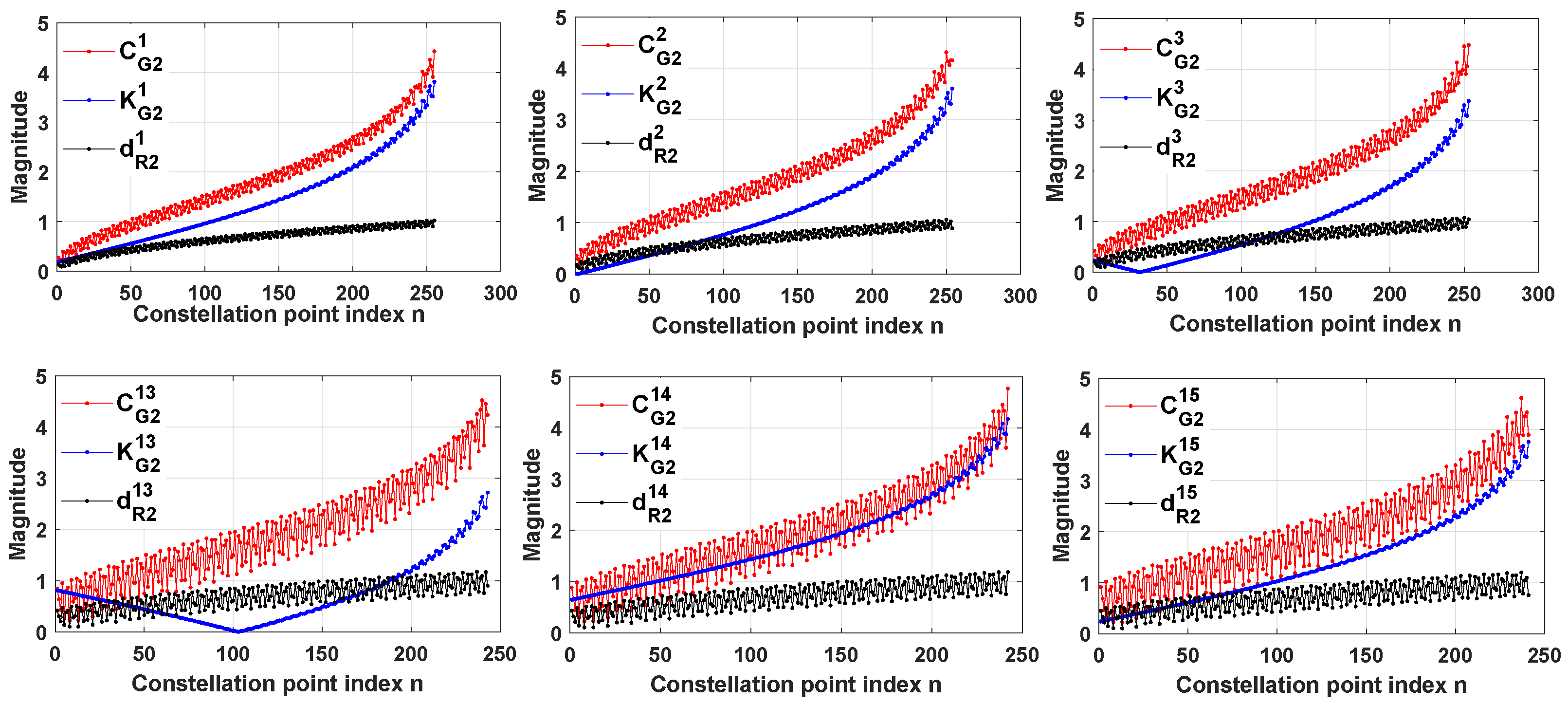
4.2. Kobayashi Pseudo-Distance of Adjacent Constellation Points

In Figure 10, we illustrate the distance performance for the Bd-GAM2 in ${\mathbb{G}}_2$ with hyper-distance (Equation (13)) in ${\mathbb{C}}^2$ and distance (Equation (14)) in Euclidean plane. The constellation size is $N=2^8$ and SNR = 22.5 dB. Select part of constellation points and calculate the distance between these points with other constellation points over different domains (e.g., distance in ${\mathbb{C}}^2$, ${\mathbb{G}}_2$, and ${\mathbb{R}}^2$ are denoted as ${\mathrm{C}}_{C2}^i$, ${\mathrm{K}}_{G2}^i$, and ${\mathrm{d}}_{R2}^i$ ($i\in \{1,2,3,13,14,15\}$)). Note that the distance for the adjacent points in ${\mathbb{G}}_2$ is always larger than the distance for the points of unit disc in Euclidean plane. The distances of adjacent points in different domains satisfy Equation (16). These constellation points keep relatively natural index order and the radial distribution of constellation points can be tuned. This avoids regions overlapping, such as phase/amplitude region. With the MI optimization problem, it is important to ensure the distance between adjacent constellation points as the modulation N increases.

Figure 10. Distance-performance for the Bd-GAM2.

Compared with the distance ${\mathrm{C}}_{C2}^i$ in ${\mathbb{C}}^2$, the distances ${\mathrm{K}}_{G2}^i$ of Bd-GAM2 in ${\mathbb{G}}_2$ decrease. The reason is that the constellation points are designed along the orbit of the boundary points. Thus, a part of constellation points (or boundary points) may have phase drift or rotation under the holomorphic mapping f. At the same time, this phenomenon can solve the geometric problem (i.e., the analytic of the expression for $r_n$) for the siganl constellation points. When the complex geometric properties, MI and power constraints are included, the inner constellation points in ${\mathbb{G}}_2$ are designed by Bd-GAM method. Using the geometric and probalilistic -shaping, we assume the signal constellation design with $r_n$ and let $p_n$ be the pmf to find the optimal scheme for constellation points.

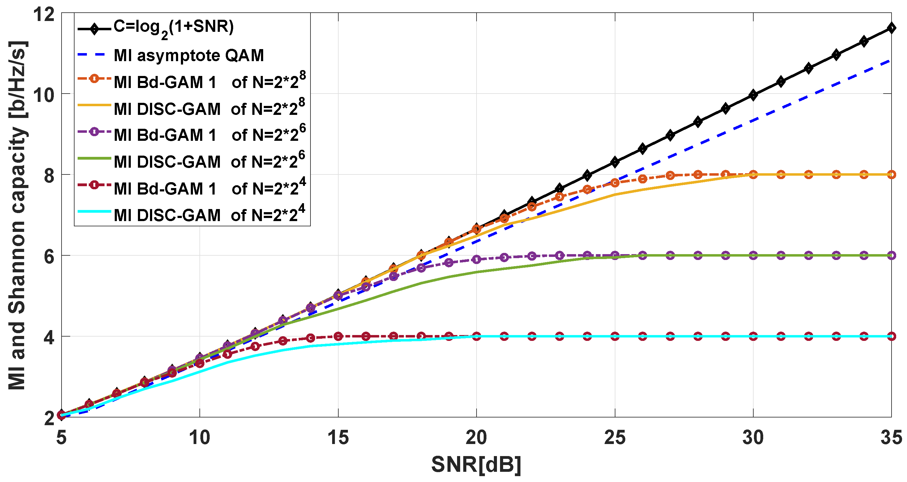
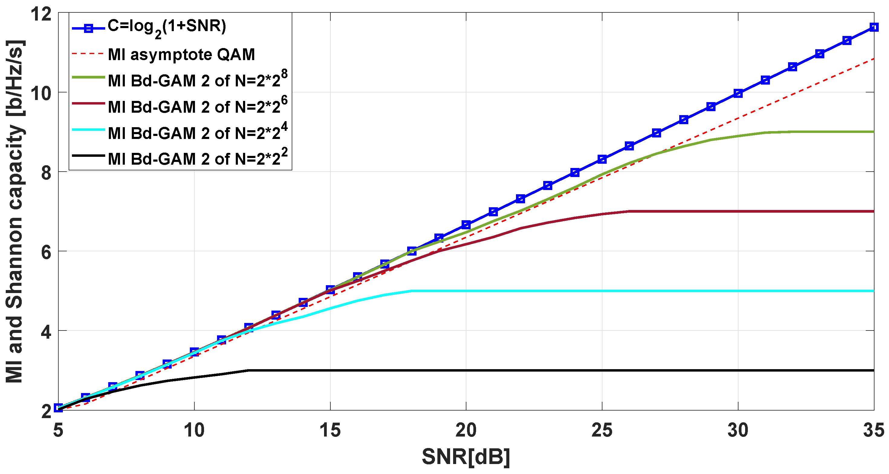
4.3. Mutual Information Performance for Bd-GAM

In this section, we present the MI-performance of Bd-GAM1/2. Monte-Carlo simulations of the MI-performance curves are used. The MI estimator [14] is defined by

$$\begin{array}{c}\hfill \widehat{I}(Y;Z)={\displaystyle \frac{1}{K}}\sum _{k=1}^K{log}_2({\displaystyle \frac{p({\mathit{y}}^{(k)}|x^{(k)})}{{\sum }_{n=1}^{N}p({\mathit{y}}^k|z_n)p(z_n)}})\end{array}$$

(30)

where K is the number of iterations. K can be defined as $K:=(k_1,k_2,k_3)$, where $k_i (i\in \{1,2,3\})$ be the number of constellation points, upper bound of $c2$ (of Equation (19)), and Levi form of $f_Y$ (of Equation (29)). z is randomly produced by $z_n$ with $p\left(z_n\right)=p_n$.

A.

Bd-GAM1

In Figure 11, we compare two different modulation methods, Bd-GAM1 [12,13] and QAM, with the AWGN Shannon capacity. The complex numerical integration is deduced in Section 3.4. The corresponding formulas are Equations (24) and (25). We can use Equations (26)–(29) to determine the orbit of the constellation points with some geometric and probalilistic -shaping. As expected, there exists a greater overlap with the AWGN Shannon capacity when the constellation points increase.

Figure 11. MI of Bd-GAM1 with $N\in \{2^4,2^6,2^8\}$.

Compared with Disc-GAM [12,13] method, Bd-GAM1 have nearly the same MI-performance as the AWGN Shannon capacity for low SNRs, and better MI-performance than Disc-GAM for high SNRs. Meanwhile, Bd-GAM1 can overcome the oscillatory phenomenon of magnitude distribution for low SNRs. The constellation size is twice that of the Disc-GAM and the additional energy consumption is required. But these costs are of less concren and in exchange for more MI-performance. Thus the Bd-GAM1 is a better optimizaiton framework, maximizing the MI under the SNR constraint.

B.

Bd-GAM2

In Figure 12, we illustrate the MI-performance for the Bd-GAM2 together with the AWGN Shannon capacity. This design implies that $H={log}_{2}N$ and we find that $H={log}_{2}N-1$ is suitable for Bd-GAM2. There exists a potential advantage for the geometric-shaping and probabilistic-shaping (i.e., entropy H and pmf $p_n$ are fixed for a given N). Note that, when the MI approaches the entropy, Bd-GAM2 performs better than QAM method. Thus, Bd-GAM2 is suboptimal for $MI\underset{\approx }{<}H-1$.

Figure 12. MI of Bd-GAM2 with $N\in \{2^3,2^5,2^7,2^9\}$.

5. Conclusions

In this paper, we have proposed a new modulation format, Bd-GAM. With complex geometric properties of open symmetrized bidisc and GAM, Bd-GAM1 and Bd-GAM2 are designed to gain more MI-performance. The theory of several complex variables has been applied to the modulation. We introduced the geometric properties of bidisc and the Levi form for the boundary constellation points in the pseudoconvex domain. By the semi-positive definiteness of the Levi form, we can find the suitable constellation points to design the modulation. Compared with the shaping-loss of QAM, Bd-GAM exhibit no asymptotic loss. For large constellations, MI optimization problems of Bd-GAM make numerical optimization computationally time consuming. As future work we plan to extend the analysis of the computational complexity to more computationally efficient optimization methods. It is hoped that more interesting applictions about the theory of several complex variables will be studied for any communication system or sparse array antennas.

References

1. Thomas, C.; Weidner, M.; Durrani, S. Digital amplitude-phase keying with M-ary alphabets. IEEE Trans. Commun. 1974, 22, 168–180. [Google Scholar] [CrossRef]
2. Hanzo, L.L.; Ng, S.X.; Keller, T.; Webb, W. Star QAM Schemes for Rayleigh fading channels. In Quadrature Amplitude Modulation: From Basics to Adaptive Trellis-Coded, Turbo-Equalised and Space-Time Coded OFDM, CDMA and MC-CDMA Systems; Wiley-IEEE Press: Hoboken, NJ, USA, 2004; pp. 307–335. [Google Scholar]
3. Forney, G.D.; Ungerboeck, G. Modulation and coding for linear Gaussian channels. IEEE Trans. Inf. Theory 1998, 44, 2384–2415. [Google Scholar] [CrossRef]
4. Betts, W.; Calderbank, A.R.; Laroian, R. Performance of non-uniform constellations on the Gaussian channel. IEEE Trans. Inf. Theory 1994, 40, 1633–1638. [Google Scholar] [CrossRef]
5. Sommer, D.; Fettweis, G.P. Signal shaping by non-uniform QAM for AWGN channels and applications using turbo coding. In Proceedings of the International ITG Conference Source and Channel Coding, Munich, Germany, 17–19 January 2000; pp. 81–86. [Google Scholar]
6. Barsoum, M.F.; Jones, C.; Fitz, M. Constellation design via capacity maximization. In Proceedings of the 2007 IEEE International Symposium on Information Theory, Nice, France, 24–29 June 2007; pp. 1821–1825. [Google Scholar]
7. Forney, G.; Gallager, R.; Lang, G.; Longstaff, F.; Qureshi, S. Efficient modulation for band-limited channels. IEEE J. Sel. Top. Signal Process. 1984, 2, 632–647. [Google Scholar] [CrossRef]
8. Calderbank, A.R.; Ozarow, L.H. Nonequiprobable signaling on the Gaussian channels. IEEE Trans. Inf. Theory 1990, 36, 726–740. [Google Scholar] [CrossRef]
9. Kschischang, F.R.; Pasupathy, S. Optimal non-uniform signaling for Gaussian channels. IEEE Trans. Inf. Theory 1993, 39, 913–929. [Google Scholar] [CrossRef]
10. Divsalar, D.; Simon, M.; Yuen, J. Trellis coding with asymmetric modulations. IEEE Trans. Commun. 1987, 35, 130–141. [Google Scholar] [CrossRef]
11. Khandani, A.K.; Kaba, P. Shaping multidimensional signal spaces. IEEE Trans. Inf. Theory 1993, 39, 1799–1808. [Google Scholar] [CrossRef]
12. Larsson, P. Golden angle modulation. IEEE Wirel. Commun. Lett. 2018, 7, 98–101. [Google Scholar] [CrossRef]
13. Larsson, P.; Rasmussen, L.K.; Skoglund, M. Golden Angle Modulation: Approaching the AWGN Capacity. arXiv 2018, arXiv:1802.10022. [Google Scholar]
14. Larsson, P. Golden angle modulation: Geometric- and probabilistic-shaping. arXiv 2017, arXiv:1708.07321. [Google Scholar]
15. Vogel, H. A better way to construct the sunflower head. Math. Biosci. 1979, 44, 179–189. [Google Scholar] [CrossRef]
16. Greene, R.E.; Kim, K.T.; Krantz, S.G. The Geometry of Complex Domains; Progress in Mathematics; Birkhäuser: Boston, MA, USA, 2011; Volume 291. [Google Scholar]
17. Agler, J.; Yeh, F.B.; Young, N.J. Realization of functions into the symmetrized bidisc. Oper. Theory Adv. Appl. 2003, 143, 1–37. [Google Scholar] [CrossRef]
18. Mheich, Z.; Wen, L.; Xiao, P.; Maaref, A. Design of SCMA Codebooks Based on Golden Angle Modulation. IEEE Trans. Veh. Technol. 2019, 68, 1501–1509. [Google Scholar] [CrossRef]
19. Larsson, P.; Rasmussen, L.K.; Skoglund, M. The Golden Quantizer: The Complex Gaussian Random Variable Case. IEEE Wirel. Commun. Lett. 2018, 143, 312–315. [Google Scholar] [CrossRef]
20. Costara, C. The symmetrized bidisc and Lempert’s theorem. Bull. Lond. Math. Soc. 2004, 36, 656–662. [Google Scholar] [CrossRef]
21. Dineen, S. The Schwarz Lemma; Oxford University Press: Oxford, UK, 1989. [Google Scholar]
22. Lempert, L. Lamétrique de Kobayashi et la représentation des domaines sur la boule. Bull. Soc. Math. Fr. 2018, 109, 427–474. [Google Scholar]
Disclaimer/Publisher’s Note: The statements, opinions and data contained in all publications are solely those of the individual author(s) and contributor(s) and not of MDPI and/or the editor(s). MDPI and/or the editor(s) disclaim responsibility for any injury to people or property resulting from any ideas, methods, instructions or products referred to in the content.
Article Metrics
Citations
Article Access Statistics
Multiple requests from the same IP address are counted as one view.