Abstract
The exact analytical solutions of a new combined Kairat-II-X differential equation are presented. The related model is investigated by combining the enhanced modified extended tanh function method and the modified -expansion method. Then, a wide range of solitary wave solutions with unknown coefficients are extracted in a variety of shapes, including dark, bright, bell-shaped, kink-type, combine, and complex solitons, exponential, hyperbolic, and trigonometric function solutions. To offer physical insight, some of the identified solutions are presented in figures. Also, 3D, 2D, and 2D density profiles of the obtained outcomes are illustrated in order to examine their dynamics with the choices of parameters involved. Based on the obtained findings, we can assert that the suggested computational approaches are efficient, dynamic, well-structured, and valuable for tackling complex nonlinear problems in several fields, including symbolic computations. The bifurcation analysis and sensitivity analysis are employed to comprehend the dynamical system. We assume that our findings will be very beneficial in improving our understanding of the waves that manifest in solids.
Keywords:
combined Kairat-II-X differential equation; analytical solutions; enhance modified extended tanh function method; modified tan(ϕ/2)-expansion method; complex nonlinear problems; bifurcation analysis MSC:
34C23; 35B32; 35C08; 35E05
1. Introduction
The majority of physical processes seen in the real world exhibit nonlinearity, and as a result, nonlinear partial differential equations (NLPDEs) were used to accurately represent complicated occurrences such as the semi-global stabilization problem of parabolic PDE-ODE systems [1], the monotone iterative and quasilinearization method [2], the dynamic complex matrix equation [3], the bifurcation diagrams and Lyapunov exponents [4], and an algorithm-based verification method [5]. It is consequently of the highest significance to researchers to find their accurate, analytical, or closed-form solutions. It is difficult to acquire these solutions since there are no conventional techniques that can be used to solve nonlinear partial differential equations. There has been a significant increase in the number of powerful methods that have been implemented in the area of developing accurate solutions for NLPDEs. Several analytical methods have been proposed for solving nonlinear evolution equations, including the -expansion method [6], the homotopy analysis method [7], the homotopy perturbation method [8], the Exp-function method [9], the Hirota bilinear method [10], the first integral method [11], the inverse scattering method [12], the Lie group method [13], the Jacobi elliptic function expansion method [14], the variational iteration method [15], the Laplace-residual power series method [16], the Legendre approximation method [17], the generalized Bogoyavlensky–Konopelchenko equation [18], the generalized Hietarinta equation [19], the dispersive wave systems [20], the variable-coefficient generalized nonlinear wave equation [21], the symmetric nonlinear dispersive wave model [22], the (3 + 1)-dimensional KPB-like equation [23], and many other methods that have yet to be identified. Some studies are full of solutions that were found after a lot of work. The research findings encompass a diverse array of solutions, including breather wave solutions, solitary wave solutions, rogue wave solutions, periodic solutions, hyperbolic solutions, and many more.
Integrable systems arise in various fields such as physics, applied mathematics, and geometry, often describing nonlinear wave phenomena, fluid dynamics, quantum [24], and other physical systems [25]. In [26], the authors proposed some new integrable systems such as Kairat equations and the Zhanbhota equation. Kairat equations can be used in wave analysis in fluid mechanics and optics. The Kairat-II equation and Kairat-X equation are represented in their standard integrable forms as follows [26]:
and
where symbolizes the wave profile. There are several studies on Equations (1) and (2) in the literature [27,28,29,30]. Very recently, Wazwaz et al. [31] proposed a new equation, Kairat-II-X, resulting from combining Equations (1) and (2). The Kairat-II-X equation is expressed as
where gives the wave field and scales the pure temporal acceleration term ; represents the advection coefficient, which physically controls the coupling between space and time evolution ; gives the higher-order dispersion coefficient, which controls third-order dispersion ; provides nonlinear interaction strength, scaling the nonlinear term ; and represents linear dispersion, controlling classical dispersion or wave stiffness. It has been demonstrated that when and the remaining parameters are redefined, Equation (3) simplifies to the Kairat-II Equation (1). Additionally, by setting , the Kairat-X Equation (2) is obtained. Thus, Equation (3) is the generalization of Equations (1) and (2). It is important to emphasize that the coefficients , and are real numbers whose magnitudes vary according to the specific model being studied. Kairat-II-X illustrates how the principles of differential geometry of curves are connected to the idea of equivalence. The Kairat-II-X equation can be used to study wave dynamics in hydrodynamics, nonlinear optics, or plasma physics.
The variational principle, Hamiltonian, solitary, and periodic wave solutions of the fractional Benjamin Ono equation were investigated in [32]. Also, a variational principle for a thin film equation was studied in [33]. Among the mentioned analytical techniques that generate soliton solutions to NLPDEs, the enhanced modified extended tanh function method (eMETFM) and the modified -expansion method (MTEM) played an important role in solving nonlinear equations. The transformation of NLPDEs to NLODEs through wave transportation enables eMETFM and MTEM, creating a set of nonlinear algebraic equations where by solving that nonlinear system, we will reach analytical solutions [34,35].
The generalized (G′/G) method, generalized projective Riccati equation method, and Riccati modified extended simple equation method were used for extracting a diverse array of soliton solutions of the Combined Kairat–II–X differential equation [36]. Wazwaz investigated two newly developed (3 + 1)-dimensional Kairat–II and Kairat–X equations that illustrate relations with the differential geometry of curves and equivalence aspects [37]. Rizvi et al. [38] studied stochastic variants of the Kairat-II and Kairat-X equations in (3 + 1)-dimensions by using the new projective Riccati equation approach of soliton solutions. The Kairat–II–X equation provided the connections between the differential geometry of curves, the concept of equivalence was applied using the Lie symmetry analysis method to investigate the vector field, and symmetry reductions of the equation were applied to find dark solitons and various combo soliton solutions in [39]. The Kairat–II equation and the Kairat–X equation were studied using , the Bernoulli Sub-ODE, and the modified auxiliary equation methods, where the constructed solutions were trigonometric, hyperbolic, exponential, and rational functions [40].
With the rapid development of nonlinear science, soliton theory has become increasingly important and lots of effective methods to develop soliton solutions have emerged [18,19,20]. Motivated by these advances, the present work employs the modified extended direct algebraic method to derive a comprehensive family of analytical solutions for a combined Kairat-II-X differential equation with constant coefficients, including bright, dark, mixed, and singular structures. Bifurcation analysis is an essential mathematical approach used to examine how the qualitative behavior of solutions in nonlinear dynamical and chaotic systems [41] evolves with changes in system parameters. In nonlinear optical wave propagation, especially in the realm of the higher-order nonlinear fractional two-mode Nizhnik–Novikov–Veselov equation and the higher-dimensional Date–Jimbo–Kashiwara–Miwa model, it offers critical understanding of the stability and dynamics of soliton solutions [42,43]. Bifurcation analysis, chaotic phenomena, the variational principle, the Hamiltonian, and solitary and periodic wave solutions of the fractional Benjamin Ono equation were investigated in [32]. Ahmed et al. [44] investigated the chaotic features of a novel variable-order fractional Rössler system with Liouville–Caputo derivatives of variable order. Dynamic, bifurcation, and Lyapunov analysis of fractional Rössler chaos were probed using the modified numerical approximation method and Laplace decomposition method [45]. The Bifurcation and sensitivity analysis, chaotic behaviors, variational principle, Hamiltonian and diverse wave solutions to investigate the extended integrable Kadomtsev-Petviashvili equation were studied in [46]. The vibration of the capillary in a nanoscale deformable tube was studied based on the variational principle and Hamiltonian [47].
In this study, we aimed to use the enhanced modified extended tanh function method, the modified -expansion method, and bifurcation analysis to investigate new combined Kairat-II-X differential equations. As demonstrated by applying the eMETFM and MTEM, generating exact, implicit solutions for this nonlinear partial differential equation turned out to be highly effective, providing clear evidence for the utility of this method in solving NLPDEs. The obtained soliton and periodic solutions can therefore provide insights into the design of stable optical transmission systems and study wave dynamics in hydrodynamics and nonlinear optics. The novelty of this work lies in extending the Kairat–X equation to include connections between the differential geometry of curves and the concept of equivalence aspects, and in employing the enhanced modified extended tanh function method and the modified -expansion method to obtain new families of analytical solutions including mixed bright–dark solitons and singular periodic structures that have not been reported in previous studies.
This paper is organized into six sections. Section 1 introduces the combined Kairat-II-X differential equation and some related nonlinear equations. The eMETFM and its application are offered in Section 2. Section 3 discusses the modified -expansion method and some exact solutions. The bifurcation analysis is analyzed in Section 4. The physical interpretation of solutions is investigated in Section 5. Section 6 provides the conclusion.
2. The eMETFM for Combined Kairat-II-X Differential Equation
This section explains the enhanced modified extended tanh function method [48]. Let the nonlinear partial differential equation be expressed as follows:
where is a function of the partial differential equations. Using the transformation , Equation (4) is transformed as
where is a function of the ordinary differential equations. According to [49], the solution of Equation (5) is obtained as
where and are constants to be determined. N is a positive integer that can be found by balancing linear and nonlinear terms in Equation (5). Function satisfies the following Riccati equation:
where is a parameter. Inserting (6) along with (7) in Equation (5) obtains the nonlinear algebra system. Solving the algebraic system of this equation, we easily obtain the required parameters.
- First Case:
Theorem 1.
Suppose ; hence, Equation (7) has hyperbolic solutions [48,49].
Proof.
When , then Riccati equation creates hyperbolic solutions with in the frame below:
□
- Second Case:
Theorem 2.
Let , then Equation (7) has trigonometric-type solutions [48,49].
Proof.
When , the Riccati equation creates trigonometric solutions with in the frame below:
□
- Third Case:
Theorem 3.
Let , then Equation (7) has a rational solution.
Proof.
When , the Riccati equation creates a rational solution in the frame below:
□
Three Types of Solutions Using eMETFM for the Combined Kairat-II-X Equation
By using the transformation wave , Equation (3) changes to
After integrating Equation (11) once with respect to , we get
Employing the principle of homogeneous balance to the terms and in Equation (12) yields . So, Equation (6) can be re-written as follows:
where and cannot be zero simultaneously. Appending Equation (13) along with Equation (7) onto Equation (12), we get the polynomial based on functions of as
Solving the above system, we get the following results:
- Solution 1:
- Solution 2:
- Solution 3:
According to (9), we obtain the trigonometric solutions
so that .
- Solution 4:
According to (9), we obtain the trigonometric solutions
so that .
- Solution 5:
According to (9), we obtain the trigonometric solutions
so that .
3. New Modified -Expansion Method
The approach of the modified -expansion method (MTEM) is related to a first-order equation. We explain the auxiliary equation below before describing the main steps of the considered technique [50]. The equation is given below:
where , are the parameters to be decided and and are fulfilled within the ODE according to
The specific arrangements of condition (29) will be examined as
- Product 1: With and , we get
- Product 2: With and , we get
- Product 3: With , , and we get
- Product 4: With , , and we get
- Product 5: With , , and we get
- Product 6: With and we get
- Product 7: With and we get
- Product 8: With , we get
- Product 9: With and , we get
- Product 10: With and , we get
- Product 11: With and , we get
To see the rest of the cases, refer to Refs. [51,52,53]. Also, , and are the values to be explored later.
Application of MTEM for the Combined Kairat-II-X Equation
According to Equation (12), which yields , Equation (28) can be re-written as follows:
Inserting Equation (12) and its derivatives into Equation (30), we get the related nonlinear arithmetical condition. The sets of solutions are as follows:
- Merge I.Through Product 9, the exact cuspon solution is
Merge II.
Through Product 5, the exact singular soliton solution is
so that and .
- Merge III.Through Product 1, the exact periodic wave solution isso that .
Through Product 2, the exact soliton solution is
so that .
- Merge IV.Through Product 9, the exact cuspon solution is
- Merge V.Through Product 5, the exact dark soliton solution isso that and .
- Merge VI.Through Product 1, the exact periodic wave solution isso that .
Through Product 2, the exact dark soliton solution is
so that .
- Merge VII.Through Product 5, the exact combined dark soliton and singular solution isso that and .
4. Bifurcation Analysis
Bifurcation analysis is important in the investigation of dynamical systems, as it explains how the qualitative behavior of a system changes in response to variations in parameters. A bifurcation occurs when a small change in the value of a parameter causes a sudden topological change in the system’s behavior. On the other hand, stability analysis is used to determine the robustness of equilibrium points in a dynamical system. Consider Equation (12) again as follows:
where and . Letting , the planner dynamics of the governing problem for Equation (47) can be expressed as
with the assessed Hamiltonian function identified as
and h characterizes a continuous variable, also called the Hamiltonian constants or energy levels. Moreover, denotes the kinetic energy, and represents the potential energy for the Hamiltonian equation (49). Critical points in the system, where no variations occur, are identified by solving the condition . For the phase portrait trajectories of the system (48), fixed points or equilibria of Equation (48) are obtained by utilizing the following results:
which becomes
Then, we have
Hence, we have two equilibrium points and with the values
So, the equilibrium points for the system (48) are and . Take the linearized form of the system (48) at equilibrium point and let
So, we can analyze the stability of these points by computing the Jacobian matrix of the system (48) as
The eigenvalues of J are given by , which implies that
where and . The following conditions are utilized:
- If the Jacobian is positive, the equilibrium point offers a center point.
- If the Jacobian is negative, the equilibrium point offers a saddle point.
- If the Jacobian is zero, the equilibrium point offers a cuspidal point. We have the following cases:
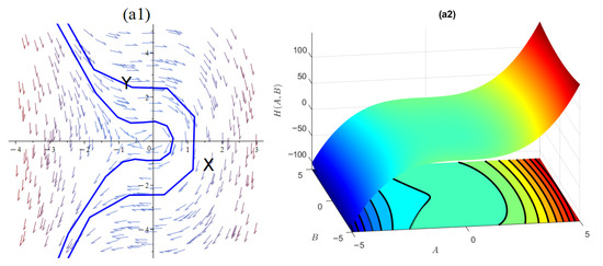
(I): and
If we obtain the amounts , and , we obtain the equilibrium points of and , where is a center point, since , and is saddle point, since , as presented in Figure 1.
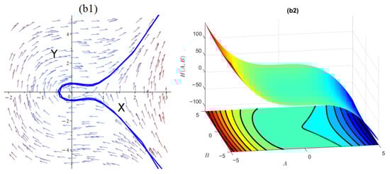
(II): and
If we obtain the amounts , and , we achieve the equilibrium points of and , where is a center point, since , and is saddle point, since , as shown in Figure 2.
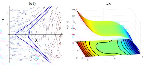
(III): and
If we obtain the amounts , and , we obtain the equilibrium points of and , where is a saddle point, since , and is saddle point, since , as shown in Figure 3.
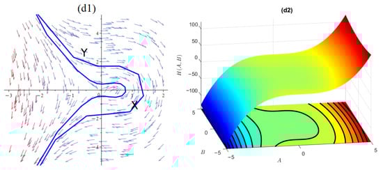
(IV): and
If we obtain the amounts , and , we achieve the equilibrium points of and , where is a saddle point, since , and is center point, since , as shown in Figure 4.
Sensitivity Analysis
This section provides a thorough examination of the sensitivity characteristics of the transformed dynamical system. A numerical approach is adopted to systematically assess how the system reacts to small perturbations in both initial conditions and system parameters. The objective is to quantify the extent to which such perturbations affect the overall evolution of the system. A sensitivity framework is developed to characterize the system’s stability. In this context, low sensitivity implies that minor variations in initial conditions result in proportionally small deviations in the system’s trajectory. To perform this sensitivity study, we solve the parametric form of the transformed dynamical model. The governing equations are represented by the following second-order system:
where the coefficients are defined in terms of system parameters as follows:
The analysis focuses on the sensitivity of the solution to controlled changes in the initial conditions and parameter values. The original system is transformed into the above planar dynamical form using a Galilean transformation, enabling a clearer examination of the solution’s behavior. To systematically evaluate the sensitivity, we consider two sets of initial conditions:
Set 1: ; ;
Set 2: ; .
Numerical simulations reveal that even slight changes in the initial state can lead to significantly different trajectories. Figure 5a illustrates the system’s response under Set 1, showing how an increase in the initial momentum leads to a shift in amplitude and phase of the resulting oscillations. Figure 5b demonstrates similar findings for Set 1, but the divergence between trajectories is more pronounced due to simultaneous variations in both and in Figure 5c and finally a variation in with constant in Figure 5d. Physically, these figures underscore the nonlinearity of the system—where even minor perturbations result in increasingly divergent trajectories over time. This reflects the inherent instability and possible chaotic behavior under specific parameter regimes. Understanding these sensitivities is vital for predicting long-term behavior and for designing control strategies in applications where precision and robustness are critical.
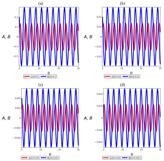
Figure 5.
Time evolution of B versus A for different initial conditions using parameters , , , , , and . (a) Sensitivity to variation in and , (b) sensitivity to variation in and , (c) sensitivity to variation in and , and (d) sensitivity to variation in with constant .
5. The Physical Interpretation of Solutions
This section aims to generate graphical illustrations of the obtained solutions of the combined Kairat-II-X differential equation, which are obtained by the eMTEFM, MTEM, and bifurcation analysis. The results showcase a variety of visual depictions, including 3D, 2D, and density plots. Here, we elaborate and investigate the dynamics of some of the obtained solutions. These results generally show dark, periodic, kink, bright, M-shaped, and W-shaped soliton solutions. The dark soliton solution (20) with suitable values is plotted in Figure 6. The behavior of soliton solution (20) with suitable values , , , , , , , is investigated in Figure 7. And the periodic wave solution (21) is designed in Figure 8 with parameters , , , , , , , . The periodic wave solution (21) with special values is plotted in Figure 9 with parameters , , , , , , , . The dark-singular soliton solution (26) with suitable values is plotted in Figure 10. The behavior of periodic soliton solution (26) with suitable values is investigated in Figure 11. And the periodic-singular wave solution (21) is designed in Figure 12 with parameters . The periodic wave solution (27) with special values is plotted in Figure 13 with parameters . We integrate the solution from Equations (15)–(46) using Maple. The results show equality between the left- and right-hand sides, confirming an exact solution. Comparison with existing literature confirms the novelty of these solutions. Bright solitons are non-dispersive wave solutions, arising in a diverse range of nonlinear, one-dimensional systems, including atomic Bose–Einstein condensates with attractive interactions. Dark solitons are defined as solutions to the nonlinear Schrödinger equation that exhibit a dip in intensity within a uniform background, characterized by an abrupt phase change at the dip center. The singular solution, in mathematics, is a solution of a differential equation that cannot be obtained from the general solution obtained by the usual method of solving the differential equation. When a differential equation is solved, a general solution consisting of a family of curves is obtained.
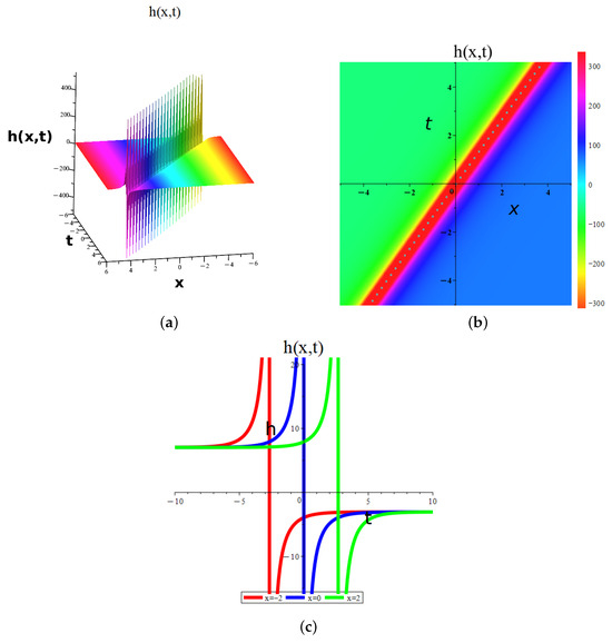
Figure 6.
Dynamic graphical visualization of the obtained result of Equation (20) of eMTEFM, giving dark soliton solutions for a (a) 3D surface, (b) 2D surface, and (c) density plot for , , , , , , , and .
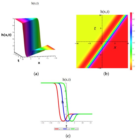
Figure 7.
Dynamic graphical visualization of the obtained result of Equation (20) of eMTEFM, giving dark-bright soliton solutions for a (a) 3D surface, (b) 2D surface, and (c) density plot for , , , and .
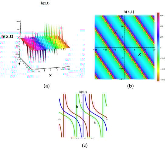
Figure 8.
Dynamic graphical visualization of the obtained result of Equation (21) of eMTEFM, giving periodic wave solutions for a (a) 3D surface, (b) 2D surface, and (c) density plot for , , and .
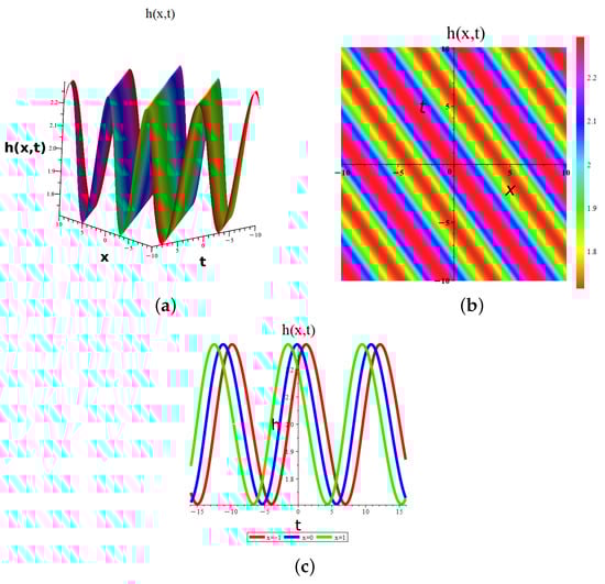
Figure 9.
Dynamic graphical visualization of the obtained result of Equation (21) of eMTEFM, giving periodic wave solutions for a (a) 3D surface, (b) 2D surface, and (c) density plot for , , and .
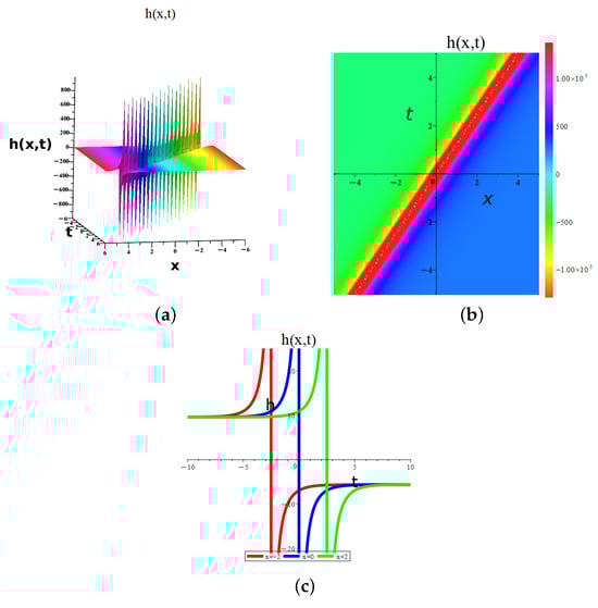
Figure 10.
Dynamic graphical visualization of the obtained result of Equation (26) of eMTEFM, giving singular soliton solutions for a (a) 3D surface, (b) 2D surface, and (c) density plot for , , , , , , , and .
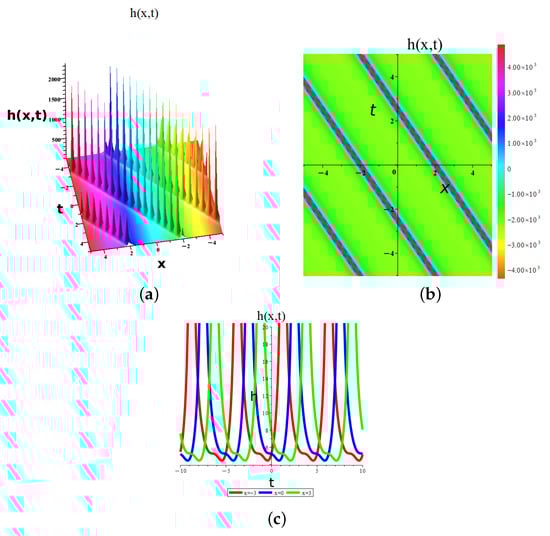
Figure 11.
Dynamic graphical visualization of the obtained result of Equation (26) of eMTEFM, giving periodic soliton solutions for a (a) 3D surface, (b) 2D surface, and (c) density plot for , , , , , , , and .
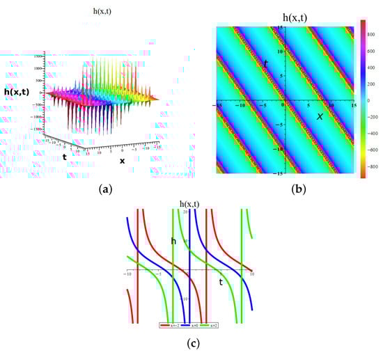
Figure 12.
Dynamic graphical visualization of the obtained result of Equation (27) of eMTEFM, giving singular periodic wave solutions for a (a) 3D surface, (b) 2D surface, and (c) density plot for and .
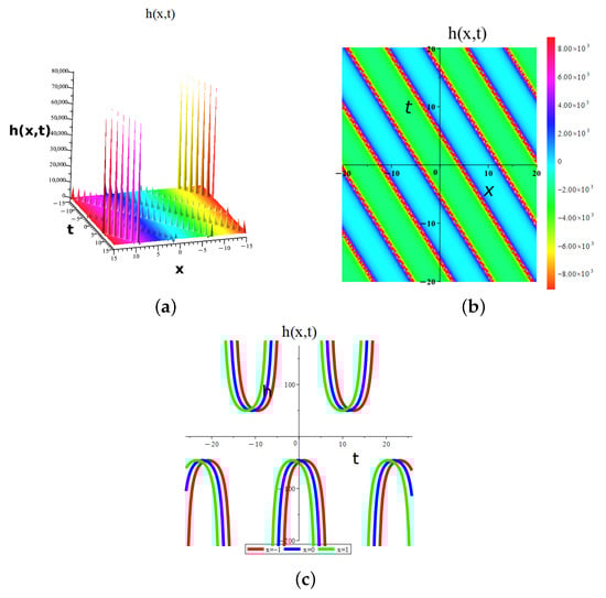
Figure 13.
Dynamic graphical visualization of the obtained result of Equation (27) of eMTEFM, giving periodic wave solutions for a (a) 3D surface, (b) 2D surface, and (c) density plot for , , , , , , , and .
6. Conclusions
We conclude that this study delivered a rigorous analytical examination of the combined Kairat-II-X differential equation. We first assessed the system with a combination of two equations. Upon validating the balance test, we introduced two novel solution techniques, the enhanced modified extended tanh function method and the modified -expansion method, to derive new soliton solutions characterized by distinct dynamic behaviors. Our analysis encompasses a comprehensive characterization of stable and functional soliton structures, including bright, dark, and periodic waves, illustrated via three-dimensional, two-dimensional, and density plots. In addition, the qualitative behavior of the dynamical system at the equilibrium points was investigated via bifurcation analysis. The bifurcation and sensitivity analysis provides crucial insights into the stability and dynamic behavior of these wave solutions under varying physical conditions. The effectiveness of these two methods in addressing the proposed model was demonstrated through both analytical methods and graphical representations, which reveal inherent periodic structures. The solutions were expressed in terms of exponential, trigonometric, and hyperbolic unctions, as well as their combinations, under specific parameter regimes. These soliton solutions offer valuable insights for both physics and mathematics. The results confirm that the employed methodologies were robust and reliable for generating a diverse set of stable, effective solutions applicable to a wide range of nonlinear partial differential equations, and they may be extended to other NLPDE models.
Author Contributions
J.Z.: Conceptualization, Methodology, Software, Writing—Original Draft Preparation; H.B.J.: Data curation, Writing—Original Draft Preparation; R.N.: Writing—Original Draft Preparation, Visualization, Investigation, Resource. All authors have read and agreed to the published version of the manuscript.
Funding
Ongoing Research Funding program (ORF-2025-210), King Saud University, Riyadh, Saudi Arabia.
Data Availability Statement
The original contributions presented in this study are included in the article. Further inquiries can be directed to the corresponding author.
Conflicts of Interest
The authors declare no conflicts of interest.
References
- Xu, X.; Li, B. Semi-global stabilization of parabolic PDE-ODE systems with input saturation. Automatica 2025, 171, 111931. [Google Scholar] [CrossRef]
- Li, Y.; Rui, Z.; Hu, B. Monotone iterative and quasilinearization method for a nonlinear integral impulsive differential equation. Aims Math. 2025, 10, 21–37. [Google Scholar]
- Jin, J.; Zhao, L.; Chen, L.; Chen, W. A robust zeroing neural network and its applications to dynamic complex matrix equation solving and robotic manipulator trajectory tracking. Front. Neurorobot. 2022, 16, 1065256. [Google Scholar] [CrossRef] [PubMed]
- Chong, Z.; Wang, C.; Zhang, H.; Zhang, S. Sine-transform-based dual-memristor hyperchaotic map and analog circuit implementation. IEEE Trans. Instrum. Meas. 2025, 74, 1–14. [Google Scholar] [CrossRef]
- Guo, X.; Zhang, J.; Meng, X.; Li, Z.; Wen, X.; Girard, P.; Yan, A. HALTRAV: Design of a high-performance and area-efficient latch With triple-node-upset recovery and algorithm-based Verifications. IEEE Trans. Comput.-Aided Des. Integr. Circuits And Syst. 2025, 44, 2367–2377. [Google Scholar]
- Lakestani, M.; Manafian, J. Analytical treatments of the space-time fractional coupled nonlinear Schrödinger equations. Opt. Quant. Elec. 2018, 50, 396. [Google Scholar]
- Dehghan, M.; Manafian, J.; Saadatmandi, A. Solving nonlinear fractional partial differential equations using the homotopy analysis method. Numer. Methods Partial. Differ. Equ. Int. J. 2010, 26, 448–479. [Google Scholar] [CrossRef]
- Dehghan, M.; Manafian, J. The solution of the variable coefficients fourth–order parabolic partial differential equations by homotopy perturbation method. Z. Naturforschung A 2009, 64a, 420–430. [Google Scholar]
- Dehghan, M.; Manafian, J.; Saadatmandi, A. Application of the Exp-function method for solving a partial differential equation arising in biology and population genetics. Int. Numer. Methods Heat Fluid Flow 2011, 21, 736–753. [Google Scholar] [CrossRef]
- Zhang, M.; Xie, X.; Manafian, J.; Ilhan, O.A.; Singh, G. Characteristics of the new multiple rogue wave solutions to the fractional generalized CBS-BK equation. J. Adv. Res. 2022, 38, 131–142. [Google Scholar]
- Liu, H.-Z. A modification to the first integral method and its applications. Appl. Math. Comput. 2022, 419, 126855. [Google Scholar] [CrossRef]
- Vakhnenko, V.O.; Parkes, E.J. The calculation of multi-soliton solutions of the vakhnenko equation by the inverse scattering method. Chaos Solitons Fractals 2002, 13, 1819–1826. [Google Scholar] [CrossRef]
- Moustafa, M.; Amin, A.M.; Laouini, G. New exact solutions for the nonlinear schrdinger’s equation with anti-cubic nonlinearity term via lie group method. Optik 2021, 248, 168205. [Google Scholar] [CrossRef]
- Liu, S.; Fu, Z.; Liu, S.; Zhao, Q. Jacobi elliptic function expansion method and periodic wave solutions of nonlinear wave equations. Phys. Lett. A 2001, 289, 69–74. [Google Scholar] [CrossRef]
- Dehghan, M.; Manafian, J. Study of the wave-breaking’s qualitative behavior of the Fornberg-Whitham equation via quasi-numeric approaches. Int. J. Num. Meth. Heat Fluid Flow 2012, 22, 537–553. [Google Scholar] [CrossRef]
- Oqielat, M.N.; Eriqat, T.; Ogilat, O.; El-Ajou, A.; Alhazmi, S.E.; Al-Omari, S. Laplace-residual power series method for solving time-fractional reaction-diffusion model. Fractal Fract. 2023, 7, 309. [Google Scholar] [CrossRef]
- Aghazadeh, A.; Mahmoudi, Y.; Saei, F.D. Legendre approximation method for computing eigenvalues of fourth order fractional Sturm-Liouville problem. Math. Comput. Simul. 2023, 206, 286–301. [Google Scholar] [CrossRef]
- Manafian, J.; Mohammadi-Ivatlo, B.; Abapour, M. Breather wave, periodic, and cross-kink solutions to the generalized Bogoyavlensky-Konopelchenko equation. Math. Meth. Appl. Sci. 2019, 43, 1753–1774. [Google Scholar] [CrossRef]
- Shen, X.; Manafian, J.; MJiang, M.; Ilhan, O.A.; Shafikk, S.S.; Zaidi, M. Abundant wave solutions for generalized Hietarinta equation with Hirota’s bilinear operator. Mod. Phys. Lett. B 2022, 36, 2250032. [Google Scholar] [CrossRef]
- Rao, X.; Manafian, J.; Mahmoud, K.H.; Hajar, A.; AB Mahdi, A.B.; Zaidi, M. The nonlinear vibration and dispersive wave systems with extended homoclinic breather wave solutions. Open Phys. 2022, 20, 795–821. [Google Scholar] [CrossRef]
- Pan, Y.; Manafian, J.; Zeynalli, S.M.; Al-Obaidi, R.; Sivaraman, R.; Kadi, A. N-Lump Solutions to a (3+1)-Dimensional Variable-Coefficient Generalized Nonlinear Wave Equation in a Liquid with Gas Bubbles. Qual. Theory Dyn. Syst. 2022, 21, 127. [Google Scholar] [CrossRef]
- Zou, Q.; Manafian, J.; Malmir, S.; Mahmoud, K.H.; Alsubaie, A.S.A.; Ewadh, N.A.; Alrekabi, I. Exact breather waves solutions in a spatial symmetric nonlinear dispersive wave model in (2+1)-dimensions. Sci. Rep. 2024, 14, 31718. [Google Scholar] [CrossRef] [PubMed]
- Gu, Y.; Zhang, X.; Huang, Z.; Peng, L.; Lai, Y.; Aminakbari, N. Soliton and lump and travelling wave solutions of the (3+1) dimensional KPB like equation with analysis of chaotic behaviors. Sci. Rep. 2024, 14, 20966. [Google Scholar] [CrossRef] [PubMed]
- Jin, Y.; Lu, G.; Liu, Y.; Sun, W. Stabilizer testing and central limit theorem. Phys. Rev. A 2025, 111, 32421. [Google Scholar] [CrossRef]
- Gu, C. (Ed.) Soliton Theory and Its Applications; Springer Science & Business Media: Berlin/Heidelberg, Germany, 2013. [Google Scholar]
- Myrzakulova, Z.; Manukure, S.; Myrzakulov, R.; Nugmanova, G. Integrability, geometry and wave solutions of some Kairat equations. arXiv 2023, arXiv:2307.00027. [Google Scholar] [CrossRef]
- Faridi, W.A.; Wazwaz, A.M.; Mostafa, A.M.; Myrzakulov, R.; Umurzakhova, Z. The Lie point symmetry criteria and formation of exact analytical solutions for Kairat-II equation: Paul-Painleve approach. Chaos Solitons Fractals 2024, 182, 114745. [Google Scholar] [CrossRef]
- Awadalla, M.; Zafar, A.; Taishiyeva, A.; Raheel, M.; Myrzakulov, R.; Bekir, A. The analytical solutions to the M-fractional Kairat-II and Kairat-X equations. Front. Phys. 2023, 11, 1335423. [Google Scholar]
- Xiao, Y.; Barak, S.; Hleili, M.; Shah, K. Exploring the dynamical behaviourofoptical solitons in integrable kairat II and kairat-X equations. Phys. Scr. 2024, 99, 095261. [Google Scholar] [CrossRef]
- Aldwoah, K.; Mustafa, A.; Aljaaidi, T.; Mohamed, K.; Alsulami, A.; Hassan, M. Exploring the impact of Brownian motion on novel closed-form solutions of the extended Kairat-II equation. PLoS ONE 2025, 20, e0314849. [Google Scholar] [CrossRef]
- Wazwaz, A.M.; Alhejaili, W.; El-Tantawy, S. Study of a combined Kairat II-X equation: Painleve integrability, multiple kink, lump and other physical solutions. Int. J. Numer. Methods Heat Fluid Flow 2024, 34, 3715–3730. [Google Scholar] [CrossRef]
- Liang, Y.H.; Wang, K.J. Bifurcation analysis, chaotic phenomena, variational principle, Hamiltonian, solitary and periodic wave solutions of the fractional Benjamin Ono equation. Fractals 2025, 33, 2550016. [Google Scholar] [CrossRef]
- He, J.H.; Sun, C. A variational principle for a thin film equation. J. Math. Chem. 2019, 57, 2075–2081. [Google Scholar] [CrossRef]
- Fugarov, D.; Dengaev, A.; Drozdov, I.; Shishulin, V.; Ostrovskaya, A. Application of tan(ϕ/2)-expansion method for solving the fractional Biswas-Milovic equation for Kerr law nonlinearity. Comput. Methods Differ. Equ. 2025, 13, 1408–1424. [Google Scholar] [CrossRef]
- Khan, U.; Irshad, A.; Ahmed, N.; Mohyud-Din, S.T. Improved tan tan(ϕ(ξ)/2)-expansion method for (2+1)-dimensional KP-BBM wave equation. Opt. Quant. Elec. 2018, 50, 135. [Google Scholar] [CrossRef]
- Younas, U.; Muhammad, J.; Ismael, H.F.; Sulaiman, T.A.; Emadifar, H.; Ahmed, K.K. The New Combined Kairat-II-X Differential Equation: Diversity of Solitary Wave Structures via New Techniques. J. Nonlinear Math. Phys. 2025, 32, 55. [Google Scholar] [CrossRef]
- Younas, U.; Muhammad, J.; Ismael, H.F.; Sulaiman, T.A.; Emadifar, H.; Ahmed, K.K. Extended (3+1)-dimensional Kairat–II and Kairat–X equations: Painlevé integrability, multiple soliton solutions, lump solutions, and breather wave solutions. Int. J. Numer. Methods Heat Fluid Flow 2024, 34, 2177–2194. [Google Scholar]
- Rizvi, S.T.R.; Jlali, L.; Anjum, I.; Abad, H.; Solouma, E.; Seadawy, A.R. Nonlinear Stochastic Wave Behavior: Soliton Solutions and Energy Analysis of Kairat-II and Kairat-X Systems. Fractal Fract. 2025, 9, 728. [Google Scholar] [CrossRef]
- Mathanaranjan, T. Lie Symmetries, Soliton Solutions, Conservation Laws, and Stability Analysis of the Combined Kairat-II-X Equation. Math. Meth. Appl. Sci. 2025, 48, 16722–16729. [Google Scholar] [CrossRef]
- Mehanna, M.S.; Wazwaz, A.M. Tri-analytical approach to Kairat–II and Kairat–X equations. Rom. Rep. Phys. 2025, 77, 107. [Google Scholar] [CrossRef]
- Liu, X.; Zhao, L.; Jin, J. A noise-tolerant fuzzy-type zeroing neural network for robust synchronization of chaotic systems. Concurr. Comput. Pract. Exp. 2024, 36, e8218. [Google Scholar] [CrossRef]
- Alam, N.; Ullah, M.S.; Manafian, J.; Mahmoud, K.H.; Alsubaie, A.S.A.; Ahmed, H.M.; Ahmed, K.K.; Khatib, S.A. Bifurcation analysis, chaotic behaviors, and explicit solutions for a fractional two-mode Nizhnik-Novikov-Veselov equation in mathematical physics. AIMS Math. 2025, 10, 4558–4578. [Google Scholar] [CrossRef]
- Tariq, K.U.; Manafian, J.; Malmir, S.; Tufail, R.N.; Ilhan, O.A.; Mahmoud, K.H. On the structure of the higher dimensional Date-Jimbo-Kashiwara-Miwa model emerging in water waves. Discov. Appl. Sci. 2025, 7, 576. [Google Scholar] [CrossRef]
- Ahmed, A.I.; Elbadri, M.; Al-Kuleab, N.; AlMutairi, D.M.; Taha, N.E.; Dafaalla, M.E. Chaos and Bifurcations in the Dynamics of the Variable-Order Fractional Rössler System. Mathematics 2025, 13, 3695. [Google Scholar] [CrossRef]
- Allogmany, R.; Alzahrani, S.S. Dynamic, Bifurcation, and Lyapunov Analysis of Fractional Rössler Chaos Using Two Numerical Methods. Mathematics 2025, 13, 3642. [Google Scholar] [CrossRef]
- Wang, K.J.; Liu, X.L.; Shi, F.; Li, G. Bifurcation and sensitivity analysis, chaotic behaviors, variational principle, Hamiltonian and diverse wave solutions of the new extended integrable Kadomtsev-Petviashvili equation. Phys. Let. A 2025, 534, 130246. [Google Scholar] [CrossRef]
- Wang, K.J.; Liu, J.H. Mathematical model and the solution of the capillary vibration in a nanoscale deformable. Math. Methods Appl. Sci. 2025, 48, 8480–8486. [Google Scholar] [CrossRef]
- Nan, T.; Manafian, J.; Ilhan, O.A.; Malmir, S.; Fattah, A.A.; Mahmoud, K.H.; Ahmed, A.M.; Nasr, Y.M. Generalized trial equation scheme and enhance modified extended tanh function method with Nonparaxial pulse propagation to the cubic-quintic nonlinear Helmholtz equation. Qual. Theory Dyn. Syst. 2025, 24, 183. [Google Scholar] [CrossRef]
- Ozisik, M.; Bayram, M.; Secer, A.; Cinar, M. On the analytical soliton solutions of (1+1)-dimensional complex coupled nonlinear Higgs field model. Eur. Phys. J. Spec. Top. 2023, 10, 1140. [Google Scholar] [CrossRef]
- Manafian, J.; Lakestani, M. Optical solitons with Biswas-Milovic equation for Kerr law nonlinearity. Eur. Phys. J. Plus 2015, 130, 61. [Google Scholar] [CrossRef]
- Gu, Y.; Manafian, J.; Malmir, S.; Eslami, B.; Ilhan, O.A. Lump, lump-trigonometric, breather waves, periodic wave and multi-waves solutions for a Konopelchenko-Dubrovsky equation arising in fluid dynamics. Int. J. Modern Phys. B 2023, 37, 2350141. [Google Scholar] [CrossRef]
- Wang, W.; Hasanirokh, K.; Manafian, J.; Abotaleb, M.; Yang, Y. Analytical approach for polar magnetooptics in multilayer spin-polarized light emitting diodes based on InAs quantum dots. Opt. Quantum Electron. 2022, 54, 137. [Google Scholar] [CrossRef]
- Ali, N.H.; Mohammed, S.A.; Manafian, J. New explicit soliton and other solutions of the Van der Waals model through the ESHGEEM and the IEEM. J. Modern Tech. Eng. 2023, 8, 5–18. [Google Scholar]


Disclaimer/Publisher’s Note: The statements, opinions and data contained in all publications are solely those of the individual author(s) and contributor(s) and not of MDPI and/or the editor(s). MDPI and/or the editor(s) disclaim responsibility for any injury to people or property resulting from any ideas, methods, instructions or products referred to in the content. |
© 2025 by the authors. Licensee MDPI, Basel, Switzerland. This article is an open access article distributed under the terms and conditions of the Creative Commons Attribution (CC BY) license (https://creativecommons.org/licenses/by/4.0/).