Reconstruction of the Initial Data and Source Functions for a Wave Equation with Nonlocal Boundary Condition

Abstract

This paper addresses multiple inverse source problems linked to the wave equation under nonlocal boundary conditions. A bi-orthogonal functional framework is adopted to represent the solutions through series expansions. The analysis establishes that these problems are ill-posed in the Hadamard sense. Three main reconstruction tasks are considered: identification of an unknown space-dependent source, recovery of the initial data, and estimation of a time-varying source term. For each case, suitable additional conditions are introduced to ensure the uniqueness of the unknown quantities. Existence and uniqueness theorems are proved under specific smoothness requirements. Finally, the theoretical developments are validated through numerical computations.

1. Introduction

In the domain

$$\mathsf{\Omega }:=\left\{\right(x,t):0<x<1,0<t<T\},$$

we study three types of inverse source problems (ISPs) associated with the wave equation

$$\begin{array}{c}\hfill U_{tt}(x,t)-U_{xx}(x,t)=F(x,t),\end{array}$$

(1)

subject to the initial conditions

$$\begin{array}{c}\hfill U(x,0)=\varphi \left(x\right),U_t(x,0)=\psi \left(x\right),x\in [0,1],\end{array}$$

(2)

and the nonlocal boundary conditions

$$\begin{array}{c}\hfill U(0,t)=0,U(1,t)+U(\alpha ,t)=0,\alpha \in (0,1),t\in [0,T].\end{array}$$

(3)

We begin by formulating the direct problem and then examine three associated ISPs derived from the given system (1)–(3).

1.1. Direct Problem (DP) 

We consider the system (1)–(3). The direct problem is to find the function $U(x,t)$. The data $\varphi \left(x\right),\psi \left(x\right)$ and $F(x,t)$ are given.

A regular solution of the direct problem is a function $U(x,t)$ such that

$$U(x,t)\in C\left(\overline{\mathsf{\Omega }}\right);\overline{\mathsf{\Omega }}=[0,1]\times [0,T],U_{xx}(·,t)\in C\left([0,1]\right),U_{tt}(x,·)\in C\left([0,T]\right).$$

1.2. Inverse Source Problem-I (ISP-I)

In ISP-I, we consider a spatially dependent source term, i.e., $F(x,t)=f\left(x\right)$, for the system (1)–(3). The objective is to determine the pair of functions $\left\{U\right(x,t),f(x\left)\right\}$. To identify the function $f\left(x\right)$, we impose the additional condition

$$\begin{array}{c}\hfill U(x,T)=\rho \left(x\right),x\in [0,1].\end{array}$$

(4)

A function pair $\left\{U\right(x,t),f(x\left)\right\}$ is referred to as a regular solution of ISP-I if it satisfies the system (1)–(3) together with the above condition and the following regularity properties:

$$f\left(x\right)\in C\left([0,1]\right),U(x,t)\in C\left(\overline{\mathsf{\Omega }}\right),U_{xx}(.,t)\in C\left([0,1]\right),U_{tt}(x,.)\in C\left([0,T]\right).$$

1.3. Inverse Source Problem-II (ISP-II)

In ISP-II, our objective is to determine the pair of functions $\left\{U\right(x,t),\varphi (x\left)\right\}$, where $\varphi \left(x\right)$ represents the unknown initial condition.

Regular solution of ISP-II is defined as the pair $\left\{U\right(x,t),\varphi (x\left)\right\}$ that satisfies the system (1)–(3) together with the additional condition (4), under the following regularity assumptions:

$$\varphi \left(x\right)\in C\left([0,1]\right),U(x,t)\in C\left(\overline{\mathsf{\Omega }}\right),U_{xx}(·,t)\in C\left([0,1]\right),U_{tt}(x,·)\in C\left([0,T]\right).$$

The additional conditions in ISP-I and ISP-II are essential for ensuring the uniqueness and stability of solutions. Specifically, the additional condition in Equation (4) serves as a necessary constraint for determining the unknown functions $f\left(x\right)$ and $\varphi \left(x\right)$. While these conditions may appear idealized, they are commonly used in practical applications such as seismology, acoustics, and medical imaging, where full data may be sparse and additional constraints are needed to recover unknown parameters. The regularity assumptions ensure that the problem remains well-posed, even with incomplete or noisy data. These conditions align with those typically used in real-world experiments, based on principles such as conservation laws or symmetry. Recent studies, such as [1,2,3], emphasize the importance of these constraints in improving the stability and convergence of ISPs.

1.4. Inverse Source Problem-III (ISP-III)

In ISP-III, the source function is expressed as $F(x,t)=a\left(t\right)f(x,t)$, where $f(x,t)$ is known, and the objective is to identify the pair $\left\{a\right(t),U(x,t\left)\right\}$ for the given system (1)–(3). To determine $a\left(t\right)$, we impose an additional integral constraint of the form

$${\int }_0^{1}U(x,t)dx=E\left(t\right),t\in [0,T].$$

(5)

The pair $\left\{a\right(t),U(x,t\left)\right\}$ is termed a regular solution of ISP-III if it fulfills the following regularity properties:

$$a\left(t\right)\in C\left([0,T]\right),U(x,t)\in C\left(\overline{\mathsf{\Omega }}\right),U_{xx}(.,t)\in C\left([0,1]\right),U_{tt}(x,.)\in C\left([0,T]\right).$$

The additional condition in ISP-III, given by the integral constraint in Equation (5), is introduced to uniquely determine the unknown function $a\left(t\right)$. This constraint ensures that the integral of the solution $U(x,t)$ over the spatial domain equals a prescribed function $E\left(t\right)$, which is often a measurable quantity in real-world applications, such as total mass or energy in physical systems. Such integral conditions are frequently employed in ISPs where global measurements are available, but the spatial distribution of the source is unknown. This condition reflects practical scenarios in fields like fluid dynamics and material science, where macroscopic quantities are easier to measure than local sources. As with ISP-I and ISP-II, the regularity assumptions on $a\left(t\right)$ and $U(x,t)$ ensure the existence and uniqueness of the solution, making the problem mathematically well-posed.

Partial differential equations (PDEs) play a central role in mathematical modeling and physical sciences, providing the framework for describing many natural and engineering processes. Among these equations, the one-dimensional wave equation is particularly important because it accurately represents the motion of wave phenomena in time and space. It is fundamental in diverse applications, including vibration analysis, acoustics, electromagnetism, and fluid mechanics. In this study, we examine the one-dimensional wave equation under specific initial and nonlocal boundary conditions to highlight how these constraints influence both the analytical formulation and the underlying physical interpretation of the model.

In mathematical modeling, nonlocal boundary conditions describe situations where the value of a system at a boundary point depends on the solution’s behavior at multiple locations within the domain, not solely on its nearby values. Such conditions typically involve integrals or derivatives evaluated over a spatial interval, introducing a nonlocal influence into the formulation. Due to this property, the spatial differential operator associated with the second boundary condition in (3) becomes non-self-adjoint, making the standard eigenfunction expansion method inapplicable. Non-self-adjoint operators often arise in models that include dissipative effects [4]. Several investigations addressing ISPs with nonlocal boundary conditions can be found in [5].

This paper focuses on the realm of ISPs, where the goal is to recover vital parameters from observed data. The first ISP centers on determining the source term $f\left(x\right)$, which characterizes the external influences driving the wave equation. The second ISP involves retrieving the initial conditions $\varphi \left(x\right)$, establishing the starting point for the wave’s evolution. Lastly, the third ISP addresses the reconstruction of the time-dependent source term, enabling the investigation of evolving external forces. These ISPs hold immense significance in practical applications, such as medical imaging [6], seismology [7], geophysics ([8,9]) and material science [10], where the ability to infer concealed properties from observable effects shapes our understanding of complex systems.

In this study, we explore ISPs for the wave equation under nonlocal boundary conditions, a topic that has not been extensively addressed in the existing literature. While ISPs in wave equations have been studied in various forms, such as identifying unknown sources or initial conditions, the use of nonlocal boundary conditions introduces challenges that are not fully covered by traditional methods. Most existing work on ISPs has focused on either local boundary conditions or methods that do not account for nonlocal influences, such as those seen in seismic or acoustic tomography (see [11]). Our work introduces a novel approach by employing a bi-orthogonal system of functions to reconstruct spatially dependent sources, initial data, and time-dependent source terms in wave equations. This method improves upon classical eigenfunction expansions, which struggle with non-self-adjoint operators that arise in nonlocal problems [12,13]. The bi-orthogonal framework offers a more robust and efficient solution to these ill-posed problems, ensuring better convergence and accuracy. Unlike conventional eigenfunction expansions, which are not directly applicable to non-self-adjoint operators, the bi-orthogonal system overcomes these limitations and enables more reliable solutions. Our contributions are distinct in that they specifically address nonlocal boundary conditions in the context of ISPs for wave equations, a topic that has been explored in various forms but not directly tackled with the same methodology or scope as in our study. The introduction of the bi-orthogonal system offers significant advantages over standard methods, such as eigenfunction expansions, which are unsuitable for non-self-adjoint operators typically encountered in nonlocal problems [14]. Furthermore, we provide a detailed theoretical analysis, including existence and uniqueness results, supported by numerical simulations that validate our findings.

Let us briefly outline the relevance of analyzing direct problems (DPs) and ISPs. A DP is well-posed, whereas an ISP is ill-posed in the sense of Hadamard, as it may lack a solution, admit multiple solutions, or exhibit instability with respect to data perturbations. The major challenge in studying such problems arises from their inherent instability. Sadybekov et al. [11] investigated nonlocal heat equations with periodic boundary conditions for DP and ISP formulations. Huntul et al. [15] recovered a time-dependent potential in a fourth-order pseudo-hyperbolic model using additional measurements. Kirane et al. [16] reconstructed a sub-diffusion process from nonlocal observations, while in another work, Kirane et al. [17] reviewed ISPs related to nonlocal wave equations with involution effects. Ahmad et al. [18] addressed the identification of a space–time fractional source term in a fractional evolution model with involution. The study in [19] addressed the joint reconstruction of the diffusion concentration profile and a time-dependent source term in a diffusion equation. Sadybekov and Sarsenbi [20] studied spectral problems related to boundary value formulations of first-order differential equations. Further investigations by Sadybekov et al. [21] analyzed the regularity of boundary problems for second-order equations with deviating arguments. Ruzhansky, Tokmagambetov, and Torebek [22] developed ISP results for hypoelliptic and subdiffusion operators. In [23], the authors discussed boundary problems for differential equations involving reflection arguments, while Burlutskaya [24] studied mixed problems with periodic and involution boundary conditions. Gupta [25] proved the existence and uniqueness of boundary value problems involving reflection of the argument.

The structure of this article is organized as follows. Section 2 introduces the spectral problem and outlines its principal results. Section 3, Section 4 and Section 5 present the formulation of the inverse source problems ISP-I, ISP-II, and ISP-III, together with the analysis of solution construction, ill-posedness, and the existence-uniqueness results for each case. In Section 6, several numerical tests corresponding to the three inverse problems are provided to illustrate the theoretical findings. The last section summarizes the key conclusions of the study.

2. Spectral Problem

In this section, we analyze the spectral characteristics of problem (1)–(3), previously examined in related literature [26]. For clarity and completeness, the spectral formulation and its associated conjugate problem corresponding to (1)–(3) can be expressed as follows:

$$X^{″}\left(x\right)+\lambda X\left(x\right)=0,X\left(0\right)=0,X\left(1\right)+X\left(\alpha \right)=0,\alpha \in (0,1),$$

(6)

$$Y^{″}\left(x\right)+\lambda Y\left(x\right)=0,Y\left(0\right)=Y\left(1\right)=Y\left[\alpha \right]=0,Y^{\prime }\left[\alpha \right]=-Y^{\prime }\left[1\right],$$

(7)

where $\lambda ={\sigma }^2$ ($Re\sigma \ge 0$) is a spectral parameter and $y\left[\alpha \right]=y(\alpha +0)-y(\alpha -0)$ denote the jump of function $y\left(x\right)$ at the point $x=\alpha$, see [26]. After resolving the problem, the following two sequences of numbers ${\sigma }_n$ and eigenfunctions of (6) are obtained:

$$\begin{array}{cc}\hfill {\sigma }_{1n}=& {\displaystyle \frac{2\pi n}{1+\alpha }},n\ge 1,X_{1n}\left(x\right)=sin\left({\sigma }_{1n}x\right),\hfill \\ \hfill {\sigma }_{2n}=& {\displaystyle \frac{\pi +2\pi n}{1-\alpha }},n\ge 0,X_{2n}\left(x\right)=sin\left({\sigma }_{2n}x\right).\hfill \end{array}$$

The eigenfunctions of (7) are given by

$$Y_{1n}\left(x\right)=\left\{{\displaystyle \begin{array}{c}{d}_{1n}sin\left({\sigma }_{1n}x\right),x\in [0,\alpha ],\hfill \\ d_{1n}\frac{cos\left({\sigma }_{1n}\alpha \right)}{2{(-1)}^{n}cos\left({\sigma }_{1n}(1-\alpha /2)\right)}(sin\left({\sigma }_{1n}x\right)-tan{\sigma }_{1n}cos\left({\sigma }_{1n}x\right)),x\in (\alpha ,1],\hfill \end{array}}\right.$$

(8)

and

$$\begin{array}{c}\hfill Y_{2n}\left(x\right)=\left\{{\displaystyle \begin{array}{c}0,x\in [0,\alpha ],\hfill \\ d_{2n}(sin\left({\sigma }_{2n}x\right)-tan{\sigma }_{2n}cos\left({\sigma }_{2n}x\right)),x\in (\alpha ,1].\hfill \end{array}}\right.\end{array}$$

The set of functions $X_{in}\left(x\right)$ and $Y_{in}\left(x\right),i=1,2,$ form a bi-orthogonal system of functions; see [26]. The variables $d_{1n}$ and $d_{2n}$ are selected to ensure the equality $⟨X_{in}\left(x\right),Y_{in}\left(x\right)⟩=1,$$i=1,2,$ holds true for all n and $⟨.,.⟩$ stand for the inner product, i.e., defined as

$$\begin{array}{c}\hfill ⟨.,.⟩={\int }_0^1{s}_1\left(x\right)s_2\left(x\right)dx.\end{array}$$

Lemma 1.

Let the function $g\left(x\right)\in C^4\left([0,1]\right)$ such that $g^m\left(0\right)=g^m\left(1\right)=0$ and $g^m\left(\alpha \right)=-g^m\left(1\right)$, $m=1,2,3$ then, we have

$$\begin{array}{cc}\hfill \mid g_{1n}\mid \le & {\displaystyle \frac{d_{1n}}{{\sigma }_{1n}^4}}\left(1+{\displaystyle \frac{cos\left({\sigma }_{1n}\alpha \right)}{{(-1)}^{n}cos\left({\sigma }_{1n}(1-\alpha /2)\right)}}\right){\parallel g^{\left(iv\right)}\left(x\right)\parallel }_{C^4\left([0,1]\right)},\hfill \\ \hfill \mid g_{2n}\mid \le & {\displaystyle \frac{2d_{2n}}{{\sigma }_{2n}^4}}{\parallel g^{\left(iv\right)}\left(x\right)\parallel }_{C^4\left([0,1]\right)},\hfill \end{array}$$

where $g_{1n}$ and $g_{2n}$ are Fourier coefficients of $g\left(x\right)$,

$$g_{1n}={\int }_0^{1}g\left(x\right)Y_{1n}\left(x\right)dx,\mathit{and}{g}_{2n}={\int }_0^{1}g\left(x\right)Y_{2n}\left(x\right)dx.$$

(9)

Proof. 

From the first part of (9), and using the value of $Y_{1n}\left(x\right)$ in (8), we have

$$\begin{array}{ccc}\hfill g_{1n}& =& {\int }_0^{\alpha }{d}_{1n}g\left(x\right)sin\left({\sigma }_{1n}x\right)dx+{\int }_{\alpha }^1{\displaystyle \frac{d_{1n}cos\left({\sigma }_{1n}\alpha \right)g\left(x\right)}{2{(-1)}^{n}cos\left({\sigma }_{1n}(1-\alpha /2)\right)}}(sin\left({\sigma }_{1n}x\right)\hfill \\ & -& tan{\sigma }_{1n}cos\left({\sigma }_{1n}x\right))dx,\hfill \\ \hfill g_{1n}:& =& {}_{\left(1\right)}g_{1n}+{}_{\left(2\right)}g_{1n}.\hfill \end{array}$$

(10)

Let

$${}_{\left(1\right)}g_{1n}={\int }_0^{\alpha }{d}_{1n}g\left(x\right)sin\left({\sigma }_{1n}x\right)dx.$$

Integrating by part the above equation, one obtains the following expression

$${}_{\left(1\right)}g_{1n}={\displaystyle \frac{d_{1n}}{{\sigma }_{1n}}}{\int }_0^{\alpha }{g}^{\prime }\left(x\right)cos\left({\sigma }_{1n}x\right)dx.$$

By repeating this process, we get

$${}_{\left(1\right)}g_{1n}={\displaystyle \frac{d_{1n}}{{\sigma }_{1n}^4}}{\int }_0^{\alpha }{g}^{\left(iv\right)}\left(x\right)sin\left({\sigma }_{1n}x\right)dx.$$

(11)

Next, we consider

$$\begin{array}{cc}\hfill {}_{\left(2\right)}g_{1n}=& {\displaystyle {\int }_{\alpha }^1\frac{d_{1n}cos\left({\sigma }_{1n}\alpha \right)g\left(x\right)}{2{(-1)}^{n}cos\left({\sigma }_{1n}(1-\alpha /2)\right)}(sin\left({\sigma }_{1n}x\right)-tan{\sigma }_{1n}cos\left({\sigma }_{1n}x\right))dx.}\hfill \end{array}$$

Integrating by part the above expression, we obtain

$$\begin{array}{cc}\hfill {}_{\left(2\right)}g_{1n}=& {\displaystyle \frac{d_{1n}cos\left({\sigma }_{1n}\alpha \right)}{2{(-1)}^{n}cos\left({\sigma }_{1n}(1-\alpha /2)\right){\sigma }_{1n}}}({\int }_{\alpha }^1{g}^{\prime }\left(x\right)cos\left({\sigma }_{1n}x\right)dx\hfill \\ \hfill -& tan{\sigma }_{1n}{\int }_{\alpha }^1{g}^{\prime }\left(x\right)sin\left({\sigma }_{1n}x\right)dx).\hfill \end{array}$$

By repeating this process, we have

$$\begin{array}{cc}\hfill {}_{\left(2\right)}g_{1n}=& {\displaystyle \frac{d_{1n}cos\left({\sigma }_{1n}\alpha \right)}{2{(-1)}^{n}cos\left({\sigma }_{1n}(1-\alpha /2)\right){\sigma }_{1n}^4}}({\int }_{\alpha }^1{g}^{\left(iv\right)}\left(x\right)sin\left({\sigma }_{1n}x\right)dx\hfill \\ \hfill -& tan{\sigma }_{1n}{\int }_{\alpha }^1{g}^{\left(iv\right)}\left(x\right)cos\left({\sigma }_{1n}x\right)dx).\hfill \end{array}$$

(12)

By plugging Equations (11) and (12) into (10), we get

$$\begin{array}{cc}\hfill g_{1n}=& {\displaystyle \frac{d_{1n}}{{\sigma }_{1n}^4}}\{{\int }_0^{\alpha }{g}^{\left(iv\right)}\left(x\right)sin\left({\sigma }_{1n}x\right)dx+{\displaystyle \frac{cos\left({\sigma }_{1n}\alpha \right)}{2{(-1)}^{n}cos\left({\sigma }_{1n}(1-\alpha /2)\right)}}\hfill \\ \hfill \times & \left({\int }_{\alpha }^1{g}^{\left(iv\right)}\left(x\right)sin\left({\sigma }_{1n}x\right)dx-tan{\sigma }_{1n}{\int }_{\alpha }^1{g}^{\left(iv\right)}\left(x\right)cos\left({\sigma }_{1n}x\right)dx\right)\}.\hfill \end{array}$$

Using the Cauchy–Schwartz inequality, we have

$$\mid g_{1n}\mid \le {\displaystyle \frac{d_{1n}}{{\sigma }_{1n}^4}}\left(1+{\displaystyle \frac{cos\left({\sigma }_{1n}\alpha \right)}{{(-1)}^{n}cos\left({\sigma }_{1n}(1-\alpha /2)\right)}}\right){\parallel g^{\left(iv\right)}\left(x\right)\parallel }_{C^4\left([0,1]\right)}.$$

Similarly, we get

$$\mid g_{2n}\mid \le {\displaystyle \frac{2d_{2n}}{{\sigma }_{2n}^4}}{\parallel g^{\left(iv\right)}\left(x\right)\parallel }_{C^4\left([0,1]\right)}.$$

□

The proof of (1) is complete.

3. Inverse Source Problem-I (ISP-I)

In the ISP-I, the source term in Equation (1) is assumed to depend only on the spatial variable, that is, $F(x,t)=f\left(x\right)$. The objective is to determine the pair of functions $\left\{U\right(x,t),f(x\left)\right\}$ satisfying the system (1)–(3) together with the additional condition (4).

3.1. Construction of the Solution of ISP-I

The eigenfunctions expansion method is used to write the solution in the form of a series as

$$\begin{array}{cc}\hfill U(x,t)=& U_{20}\left(t\right)X_{20}\left(x\right)+\sum _{n=1}^{\infty }\left[\sum _{j=1}^2\left(U_{jn}\left(t\right)X_{jn}\left(x\right)\right)\right],\hfill \end{array}$$

(13)

$$\begin{array}{cc}\hfill f\left(x\right)=& f_{20}{X}_{20}\left(x\right)+\sum _{n=1}^{\infty }\left[\sum _{j=1}^2\left(f_{jn}{X}_{jn}\left(x\right)\right)\right],\hfill \end{array}$$

(14)

where the temporal functions $U_{20}\left(t\right)$ and $U_{jn}\left(t\right)$ for $j=1,2$, together with the coefficients $f_{20}$ and $f_{jn}$ for $j=1,2$, are the unknown quantities to be evaluated. Using the bi-orthogonality property of the basis functions, Equation (13) can be reformulated as

$$U_{20}\left(t\right)=⟨U(x,t),Y_{20}\left(x\right)⟩.$$

From Equation (1), the following ordinary differential equation is obtained

$$\begin{array}{c}\hfill U_{20}^{″}\left(t\right)=-{\sigma }_{20}{U}_{20}\left(t\right)+f_{20}.\end{array}$$

(15)

Similarly, we can obtain the following expression:

$$\begin{array}{c}\hfill U_{jn}^{″}\left(t\right)=-{\sigma }_{jn}{U}_{jn}\left(t\right)+f_{jn},j=1,2.\end{array}$$

(16)

Applying Laplace transform (LT) on (15) and initial conditions (2), we obtain

$$\mathcal{L}\{U_{20}\left(t\right);s\}={\displaystyle \frac{s{\varphi }_{20}}{s^2+{\sigma }_{20}}}+{\displaystyle \frac{{\psi }_{20}}{s^2+{\sigma }_{20}}}+{\displaystyle \frac{f_{20}}{s(s^2+{\sigma }_{20})}},$$

(17)

where

$$\begin{array}{c}\hfill {\varphi }_{20}=⟨\varphi \left(x\right),Y_{20}\left(x\right)⟩,\mathit{and}{\psi }_{20}=⟨\psi \left(x\right),Y_{20}\left(x\right)⟩.\end{array}$$

Taking the inverse LT in (17), then we get the following expression

$$\begin{array}{cc}\hfill U_{20}\left(t\right)=& {\varphi }_{20}cos\left(\sqrt{{\sigma }_{20}}t\right)+{\psi }_{20}\sqrt{{\sigma }_{20}}sin\left(\sqrt{{\sigma }_{20}}t\right)+f_{20}\sqrt{{\sigma }_{20}}{\int }_0^{t}sin\left(\sqrt{{\sigma }_{20}}\tau \right)d\tau .\hfill \end{array}$$

(18)

Similarly, using the LT technique of (16) and initial conditions (2), we have

$$\begin{array}{cc}\hfill U_{jn}\left(t\right)=& {\varphi }_{jn}cos\left(\sqrt{{\sigma }_{jn}}t\right)+{\psi }_{jn}\sqrt{{\sigma }_{jn}}sin\left(\sqrt{{\sigma }_{jn}}t\right)+f_{jn}\sqrt{{\sigma }_{jn}}{\int }_0^{t}sin\left(\sqrt{{\sigma }_{jn}}\tau \right)d\tau ,\hfill \end{array}$$

(19)

$j=1,2.$ Additionally, ${\varphi }_{jn}$, and ${\psi }_{jn},j=1,2$ are the coefficients of the series expansion of $\varphi \left(x\right)$ and $\psi \left(x\right)$, and these are defined as follows:

$$\begin{array}{c}\hfill {\varphi }_{jn}=⟨\varphi \left(x\right),Y_{jn}\left(x\right)⟩,\mathit{and}{\psi }_{jn}=⟨\psi \left(x\right),Y_{jn}\left(x\right)⟩.\end{array}$$

Due to the additional condition (4) and the results of Equations (18) and (19), we have

$$\begin{array}{c}\hfill f_{20}={\displaystyle \frac{{\rho }_{20}-{\varphi }_{20}cos\left(\sqrt{{\sigma }_{20}}T\right)-{\psi }_{20}\sqrt{{\sigma }_{20}}sin\left(\sqrt{{\sigma }_{20}}T\right)}{{\displaystyle \sqrt{{\sigma }_{20}}{\int }_0^{T}sin\left(\sqrt{{\sigma }_{20}}\tau \right)d\tau }}},\end{array}$$

(20)

$$\begin{array}{c}\hfill f_{jn}={\displaystyle \frac{{\rho }_{jn}-{\varphi }_{jn}cos\left(\sqrt{{\sigma }_{jn}}T\right)-{\psi }_{jn}\sqrt{{\sigma }_{jn}}sin\left(\sqrt{{\sigma }_{jn}}T\right)}{{\displaystyle \sqrt{{\sigma }_{jn}}{\int }_0^{T}sin\left(\sqrt{{\sigma }_{jn}}\tau \right)d\tau }}},j=1,2,\end{array}$$

(21)

where the series expansion coefficients of $\rho \left(x\right)$ are ${\rho }_{20}$, and ${\rho }_{jn},j=1,2$, and these are defined as

$$\begin{array}{c}\hfill {\rho }_{20}=⟨\rho \left(x\right),Y_{20}\left(x\right)⟩,\mathit{and}{\rho }_{jn}=⟨\rho \left(x\right),Y_{jn}\left(x\right)⟩.\end{array}$$

3.2. Ill-Posedness of ISP-I

In this section, the instability characteristics of ISP-I are examined. To support the analysis, several auxiliary lemmas are first presented.

Lemma 2

([16]). For $0<\eta <1,\tau ,\sigma >0,$ we have $0<E_{\eta ,1}(\tau ,\sigma )<1.$ Moreover $E_{\eta ,1}(\tau ,\sigma )$ is completely monotonic that is

$$\begin{array}{c}\hfill {(-1)}^n{\left[E_{\eta ,1}(\tau ,\sigma )\right]}^{\left(n\right)}\ge 0,\forall n\in N.\end{array}$$

Lemma 3

([27]). If $\eta <2,\alpha$ is an arbitrary real number, μ is such that $\pi \alpha /2<\mu <min\{\pi ,\pi \alpha \},$ $z\in \mathbb{C}$ such that $\left|z\right|\ge 0,$ $\mu \le \left|arg\right(z\left)\right|\le \pi$ and $D_1$ is a real constant, then

$$\begin{array}{c}\hfill |E_{\eta ,\alpha }\left(z\right)|\le {\displaystyle \frac{D_1}{1+\left|z\right|}}.\end{array}$$

Consider an example to illustrate the instability of ISP-I. Assume the final and initial data are given by

$$\begin{array}{c}\hfill \tilde{\rho }\left(x\right)={\displaystyle \frac{1}{\sqrt{{\sigma }_{in}}}}sin\left({\sigma }_{in}x\right),\tilde{\varphi }\left(x\right)=\tilde{\psi }\left(x\right)=0,i=1,2.\end{array}$$

The corresponding source function becomes

$$\begin{array}{c}\hfill \tilde{f}\left(x\right)={\displaystyle \frac{1}{{\displaystyle {\sigma }_{in}{\int }_0^{T}sin\left(\sqrt{{\sigma }_{in}\tau }\right)d\tau }}}sin\left({\sigma }_{in}x\right).\end{array}$$

Next, consider another case with the final data $\rho \left(x\right)=0$ and the same initial conditions $\varphi \left(x\right)=\psi \left(x\right)=0$, which gives $f\left(x\right)=0$. We now compute the $L^2$-error between the two sets of final data:

$$\begin{array}{c}\hfill \parallel \tilde{\rho }{-\rho \parallel }_{L^2(0,1)}=\parallel {\displaystyle \frac{1}{\sqrt{{\sigma }_{in}}}}{\parallel }_{L^2(0,1)}={\displaystyle \frac{1}{\sqrt{{\sigma }_{in}}}}.\end{array}$$

Thus,

$$\begin{array}{c}\hfill \underset{n\to \infty }{lim}{\parallel \tilde{\rho }-\rho \parallel }_{L^2(0,1)}=\underset{n\to \infty }{lim}{\displaystyle \frac{1}{\sqrt{{\sigma }_{in}}}}=0.\end{array}$$

Additionally, by determining the norm error between the corresponding source terms, we obtain

$$\begin{array}{cc}\hfill \parallel \tilde{f}{-f\parallel }_{L^2(0,1)}=& \parallel {\displaystyle \frac{1}{{\sigma }_{in}{\int }_0^{T}sin\left(\sqrt{{\sigma }_{in}\tau }\right)d\tau }}sin\left({\sigma }_{in}x\right){\parallel }_{L^2(0,1)}\hfill \\ \hfill =& {\displaystyle \frac{1}{2{\sigma }_{in}{\int }_0^{T}sin\left(\sqrt{{\sigma }_{in}\tau }\right)d\tau }}\left(1-{\displaystyle \frac{sin\left(2{\sigma }_{in}\right)}{2{\sigma }_{in}}}\right).\hfill \end{array}$$

From Lemma 2, we have

$$\begin{array}{cc}\hfill {\int }_0^{T}sin\left(\sqrt{{\sigma }_{in}\tau }\right)d\tau =& \sqrt{{\sigma }_{in}}{t}^2{E}_{2,3}(-{\sigma }_{in}t)={\displaystyle \frac{1}{\sqrt{{\sigma }_{in}}}}{\int }_0^T{\displaystyle \frac{d}{ds}}{E}_{2,1}(-{\sigma }_{in}{s}^2)ds\hfill \\ \hfill =& {\displaystyle \frac{1-E_{2,1}(-{\sigma }_{in}{T}^2)}{{\sigma }_{in}}}\le {\displaystyle \frac{1}{{\sigma }_{in}}}.\hfill \end{array}$$

(22)

By using the estimate of (22), we obtain

$$\begin{array}{c}\hfill \parallel \tilde{f}{-f\parallel }_{L^2(0,1)}\ge \left(1-{\displaystyle \frac{sin\left(2{\sigma }_{in}\right)}{2{\sigma }_{in}}}\right),\end{array}$$

Hence,

$$\begin{array}{c}\hfill \underset{n\to \infty }{lim}{\parallel \tilde{f}-f\parallel }_{L^2(0,1)}\ge \underset{n\to \infty }{lim}\left(1-{\displaystyle \frac{sin\left(2{\sigma }_{in}\right)}{2{\sigma }_{in}}}\right)=-\infty .\end{array}$$

(23)

From (23), we assume that ISP-I is ill-posed.

3.3. Existence of the Solution of ISP-I

We now recall a useful auxiliary result that will be employed in the subsequent analysis.

Lemma 4

([28]). Let $h\in C^1\left([0,T]\right)$ and $\lambda \in \mathbb{R}\setminus \left\{0\right\}$. Then there exists a constant $C_1>0$ such that

$$\left|(h\ast sin\left(\sqrt{{\sigma }_{jn}t}\right))\left(t\right)\right|\le {\displaystyle \frac{C_1}{|{\sigma }_{jn}|}}{\parallel h\parallel }_{C^1\left([0,T]\right)},j=1,2,$$

(24)

where ${\displaystyle {\parallel h\parallel }_{C^1\left([0,T]\right)}=\underset{0\le t\le T}{max}\left|h\left(t\right)\right|}$, and the operator ∗ denotes the Laplace convolution defined by

$$(f\ast g)\left(t\right)={\int }_0^{t}f(t-\tau )g\left(\tau \right)d\tau .$$

Theorem 1.

There exists a regular solution of IP-I, if $\varphi \left(x\right)\in C^4\left([0,1]\right)$, $\psi \left(x\right)\in C^4\left([0,1]\right)$, $\rho \left(x\right)\in C^4\left([0,1]\right)$ and the function $\varphi \left(x\right)$, $\psi \left(x\right)$ and $\rho \left(x\right)$ satisfy the following conditions:

1. 

${\varphi }^m\left(0\right)={\varphi }^m\left(1\right)=0$ and ${\varphi }^m\left(\alpha \right)=-{\varphi }^m\left(1\right)$, $m=1,2,3$;

2. 

${\psi }^m\left(0\right)={\psi }^m\left(1\right)=0$ and ${\psi }^m\left(\alpha \right)=-{\psi }^m\left(1\right)$, $m=1,2,3$;

3. 

${\rho }^m\left(0\right)={\rho }^m\left(1\right)=0$ and ${\rho }^m\left(\alpha \right)=-{\rho }^m\left(1\right)$, $m=1,2,3$;

4. 

${\displaystyle \frac{1}{|{\int }_0^{T}sin\left({\sigma }_{in}\tau \right)d\tau |}\le C_2,T>0,i=1,2.}$

Proof. 

For establishing the existence result stated in Theorem 1, it is required to demonstrate the uniform convergence of the involved series $U(x,t)$, $f\left(x\right)$, $U_{tt}(x,t)$, and $U_{xx}(x,t)$. We begin with the convergence of $f\left(x\right)$. From expression (21) with $j=1$, we have

$$\begin{array}{c}\hfill |f_{1n}|=\left|{\displaystyle \frac{{\rho }_{1n}-{\varphi }_{1n}cos\left(\sqrt{{\sigma }_{1n}}T\right)-{\psi }_{1n}\sqrt{{\sigma }_{1n}}sin\left(\sqrt{{\sigma }_{1n}}T\right)}{{\displaystyle \sqrt{{\sigma }_{1n}}{\int }_0^{T}sin\left(\sqrt{{\sigma }_{1n}}\tau \right)d\tau }}}\right|.\end{array}$$

Since

$$cos\left(\sqrt{{\sigma }_{1n}}T\right)<1,\mathit{and}sin\left(\sqrt{{\sigma }_{1n}}T\right)<1,$$

the above expression gives

$$\begin{array}{c}\hfill |f_{1n}|\le {\displaystyle \frac{C_2}{\sqrt{{\sigma }_{1n}}}}\left(|{\rho }_{1n}|-|{\varphi }_{1n}|-|{\psi }_{1n}|\sqrt{|{\sigma }_{1n}|}\right).\end{array}$$

Using Lemma 1, we obtain

$$\begin{array}{cc}\hfill \mid f_{1n}\mid \le & {\displaystyle \frac{C_2{d}_{1n}}{|{\sigma }_{1n}{|}^{9/2}}}\left(1+{\displaystyle \frac{cos\left({\sigma }_{1n}\alpha \right)}{{(-1)}^{n}cos\left({\sigma }_{1n}(1-\alpha /2)\right)}}\right)({\parallel {\rho }^{\left(iv\right)}\left(x\right)\parallel }_{C^4\left([0,1]\right)}\hfill \\ \hfill +& \parallel {\varphi }^{\left(iv\right)}{\left(x\right)\parallel }_{C^4\left([0,1]\right)}+\sqrt{{\sigma }_{1n}}{\parallel {\psi }^{\left(iv\right)}\left(x\right)\parallel }_{C^4\left([0,1]\right)}).\hfill \end{array}$$

(25)

Similarly, by using Lemma 1 and (21) for $j=2$, we get

$$|f_{2n}|\le {\displaystyle \frac{2C_2{d}_{2n}}{|{\sigma }_{2n}{|}^{9/2}}}\left(\parallel {\rho }^{\left(iv\right)}{\left(x\right)\parallel }_{C^4\left([0,1]\right)}+\parallel {\varphi }^{\left(iv\right)}{\left(x\right)\parallel }_{C^4\left([0,1]\right)}+\sqrt{{\sigma }_{2n}}{\parallel {\psi }^{\left(iv\right)}\left(x\right)\parallel }_{C^4\left([0,1]\right)}\right).$$

(26)

From inequalities (25) and (26), it follows that the series expansion of $f\left(x\right)$ defines a continuous function. This result is established through the application of the Weierstrass M-test.

Next, we establish the uniform convergence of $U(x,t)$. From the expression (19) with $j=1$, we have

$$\begin{array}{cc}\hfill |U_{1n}\left(t\right)|=& \left|{\varphi }_{1n}cos\left(\sqrt{{\sigma }_{1n}}t\right)+{\psi }_{1n}\sqrt{{\sigma }_{1n}}sin\left(\sqrt{{\sigma }_{1n}}t\right)+f_{1n}\sqrt{{\sigma }_{1n}}{\int }_0^{t}sin\left(\sqrt{{\sigma }_{1n}}\tau \right)d\tau \right|,\hfill \end{array}$$

We know that

$$cos\left(\sqrt{{\sigma }_{1n}}T\right)<1,\mathit{and}sin\left(\sqrt{{\sigma }_{1n}}T\right)<1.$$

Using Lemma 4, the above expression yields

$$\begin{array}{cc}\hfill |U_{1n}\left(t\right)|\le & |{\varphi }_{1n}|+|{\psi }_{1n}|\sqrt{|{\sigma }_{1n}|}+\left|f_{jn}\right|{\displaystyle \frac{C_1}{\sqrt{|{\sigma }_{1n}|}}},\hfill \end{array}$$

Due to Lemma 1, we obtain

$$\begin{array}{cc}\hfill |U_{1n}\left(t\right)|\le & {\displaystyle \frac{d_{1n}}{|{\sigma }_{1n}{|}^4}}\left(1+{\displaystyle \frac{cos\left({\sigma }_{1n}\alpha \right)}{{(-1)}^{n}cos\left({\sigma }_{1n}(1-\alpha /2)\right)}}\right)({\parallel {\varphi }^{\left(iv\right)}\left(x\right)\parallel }_{C^4\left([0,1]\right)}\hfill \\ \hfill +& \sqrt{|{\sigma }_{1n}|}{\parallel {\psi }^{\left(iv\right)}\left(x\right)\parallel }_{C^4\left([0,1]\right)})+{\displaystyle \frac{C_1}{\sqrt{|{\sigma }_{1n}|}}}\mid f_{1n}\mid .\hfill \end{array}$$

(27)

Similarly, for $j=2$, one gets the following inequality:

$$\mid U_{2n}\left(t\right)\mid \le {\displaystyle \frac{2C_2{d}_{2n}}{|{\sigma }_{2n}{|}^{9/2}}}\left(\parallel {\varphi }^{\left(iv\right)}{\left(x\right)\parallel }_{C^4\left([0,1]\right)}+{\parallel {\psi }^{\left(iv\right)}\left(x\right)\parallel }_{C^4\left([0,1]\right)}\right)+{\displaystyle \frac{C_1}{|{\sigma }_{2n}{|}^{3/2}}}\left|f_{2n}\right|.$$

(28)

From Equations (27) and (28), the series expression $U(x,t)$ in Equation (13) is shown to converge uniformly as verified through the Weierstrass M-test.

Next, we verify that $U_{tt}(x,t)$ defines a continuous function. To examine the uniform convergence of $U_{tt}(x,t)$, we differentiate Equation (13) twice with respect to the time variable t

$$U_{tt}(x,t)=U_{20}^{″}\left(t\right)X_{20}\left(x\right)+\sum _{n=1}^{\infty }\left[\sum _{j=1}^2\left(U_{jn}^{″}\left(t\right)X_{jn}\left(x\right)\right)\right],$$

(29)

where

$$\begin{array}{c}\hfill U_{20}^{″}\left(t\right)=-{\sigma }_{20}cos\left(\sqrt{{\sigma }_{20}}t\right){\varphi }_{20}-{\psi }_{20}{\sigma }_{20}^{3/2}sin\left(\sqrt{{\sigma }_{20}}t\right)+f_{2,0}{\sigma }_{20}cos\left(\sqrt{{\sigma }_{20}}t\right)),\end{array}$$

$$\begin{array}{c}\hfill U_{jn}^{″}\left(t\right)=-\left({\sigma }_{jn}cos\left(\sqrt{{\sigma }_{jn}}t\right){\varphi }_{jn}+{\psi }_{j,n}{\sigma }_{jn}^{3/2}sin\left(\sqrt{{\sigma }_{jn}}t\right)-f_{1n}{\sigma }_{j,n}cos\left(\sqrt{{\sigma }_{jn}}t\right)\right).\end{array}$$

Taking the absolute of the above equality for $j=1,2$ and using Lemmas 1 and 4, we get

$$\begin{array}{cc}\hfill |U_{1n}^{″}\left(t\right)|\le & {\displaystyle \frac{d_{1n}}{|{\sigma }_{1n}{|}^3}}\left(1+{\displaystyle \frac{cos\left({\sigma }_{1n}\alpha \right)}{{(-1)}^{n}cos\left({\sigma }_{1n}(1-\alpha /2)\right)}}\right)({\parallel {\varphi }^{\left(iv\right)}\left(x\right)\parallel }_{C^4\left([0,1]\right)}\hfill \\ \hfill +& \sqrt{|{\sigma }_{1n}|}{\parallel {\psi }^{\left(iv\right)}\left(x\right)\parallel }_{C^4\left([0,1]\right)})+{\displaystyle \frac{C_1}{|{\sigma }_{1n}|}}\mid f_{1n}\mid \hfill \\ \hfill |U_{2n}^{″}\left(t\right)|\le & {\displaystyle \frac{2d_{2n}}{|{\sigma }_{{2n|}^3}}}\left(\parallel {\varphi }^{\left(iv\right)}{\left(x\right)\parallel }_{C^4\left([0,1]\right)}+\sqrt{|{\sigma }_{2n}|}{\parallel {\psi }^{\left(iv\right)}\left(x\right)\parallel }_{C^4\left([0,1]\right)}\right)+{\displaystyle \frac{C_1}{|{\sigma }_{2n}|}}\left|f_{2n}\right|.\hfill \end{array}$$

From the above bounds for $|U_{1n}^{″}\left(t\right)|$ and $|U_{2n}^{″}\left(t\right)|$, it follows that the series representation of $U_{tt}(x,t)$ in Equation (29) converges uniformly. Hence, by the Weierstrass M-test, $U_{tt}(x,t)$ defines a continuous function.

To verify the continuity of $U_{xx}(x,t)$, we differentiate Equation (13) twice with respect to x

$$U_{xx}(x,t)=U_{20}\left(t\right)X_{20}^{″}\left(x\right)+\sum _{n=1}^{\infty }\left[\sum _{j=1}^2\left(U_{jn}\left(t\right)X_{jn}^{″}\left(x\right)\right)\right].$$

By taking the absolute of above expression, using Lemmas 1 and 4, one gets

$$\begin{array}{cc}\hfill |U_{xx}(x,t)|\le & \sum _{n=1}^{\infty }\left[{\displaystyle \frac{d_{1n}}{|{\sigma }_{1n}{|}^2}}\left(1+{\displaystyle \frac{cos\left({\sigma }_{1n}\alpha \right)}{{(-1)}^{n}cos\left({\sigma }_{1n}(1-\alpha /2)\right)}}\right)\right({\parallel {\varphi }^{\left(iv\right)}\left(x\right)\parallel }_{C^4\left([0,1]\right)}\hfill \\ \hfill +& \parallel {\psi }^{\left(iv\right)}{\left(x\right)\parallel }_{C^4\left([0,1]\right)})+\sqrt{|{\sigma }_{1n}|}{C}_1\mid f_{1n}\mid +{\displaystyle \frac{2d_{2n}}{|{\sigma }_{2n}{|}^2}}({\parallel {\varphi }^{\left(iv\right)}\left(x\right)\parallel }_{C^4\left([0,1]\right)}\hfill \\ \hfill +& \parallel {\psi }^{\left(iv\right)}{\left(x\right)\parallel }_{C^4\left([0,1]\right)})+C_1\sqrt{|{\sigma }_{2n}|}\left|f_{2n}\right|].\hfill \end{array}$$

By applying the Weierstrass M-test, it follows that the series representing $U_{xx}(x,t)$ converges uniformly. □

Remark 1.

For the DP governed by Equations (1)–(3), where the function $F(x,t)$ in Equation (1) is known, one can establish the existence of a solution using the same reasoning as before. The result is summarized below.

Theorem 2.

Assume that the following conditions hold:

(C1) 

$\varphi \left(x\right)\in C^4\left([0,1]\right)$, ${\varphi }^m\left(0\right)={\varphi }^m\left(1\right)=0$ and ${\varphi }^m\left(\alpha \right)=-{\varphi }^m\left(1\right)$, $m=1,2,3$;

(C2) 

$\psi \left(x\right)\in C^4\left([0,1]\right)$, ${\psi }^m\left(0\right)={\psi }^m\left(1\right)=0$ and ${\psi }^m\left(\alpha \right)=-{\psi }^m\left(1\right)$, $m=1,2,3$;

(C3) 

$F(x,t)\in C^4\left([0,1]\right)$, $F^m(0,t)=F^m(1,t)=0$ and $F^m(\alpha ,t)=-F^m(1,t)$, $m=1,2,3$.

Given these assumptions, a regular solution to the DP for the system (1)–(3) exists.

3.4. Uniqueness of the Solution of ISP-I

Theorem 3.

Let $\left\{U\right(x,t),f(x\left)\right\}$ and $\{\widehat{U}(x,t),\widehat{f}\left(x\right)\}$ be two regular solutions of the ISP-I. If there exists a point $x_0\in (0,1)$ such that $U(x_0,t)=\widehat{U}(x_0,t)$ for all $t\in [0,T]$, then it follows that $U(x,t)=\widehat{U}(x,t)$ and $f\left(x\right)=\widehat{f}\left(x\right)$ for every $x\in (0,1)$ and $(x,t)\in \mathsf{\Omega }$.

Proof. 

Suppose the following functions are defined:

$$U_{20}\left(t\right)={\int }_0^{1}U(x,t)Y_{20}\left(x\right)dx,\mathit{and}{\tilde{U}}_{20}\left(t\right)={\int }_0^1\tilde{U}(x,t)Y_{20}\left(x\right)dx.$$

Similarly, we define

$$\begin{array}{cc}\hfill U_{jn}\left(t\right)=& {\int }_0^{1}U(x,t)Y_{jn}\left(x\right)dx,\hfill \end{array}$$

(30)

$$\begin{array}{cc}\hfill {\tilde{U}}_{jn}\left(t\right)=& {\int }_0^1\tilde{U}(x,t)Y_{jn}\left(x\right)dx,j=1,2.\hfill \end{array}$$

(31)

Taking twice derivative on both sides of Equation (30), then by virtue of (1), using LT and initial conditions (2), we have

$$U_{jn}\left(t\right)={\varphi }_{jn}cos\left(\sqrt{{\sigma }_{jn}}t\right)+\sqrt{{\sigma }_{jn}}{\psi }_{jn}sin\left(\sqrt{{\sigma }_{jn}}t\right)+\sqrt{{\sigma }_{jn}}{f}_{jn}\left({\int }_0^{t}sin\left(\sqrt{{\sigma }_{jn}}\tau \right)d\tau \right).$$

Similarly, one obtains the following expression for the equation given in (31)

$${\tilde{U}}_{jn}\left(t\right)={\varphi }_{jn}cos\left(\sqrt{{\sigma }_{jn}}t\right)+\sqrt{{\sigma }_{jn}}{\psi }_{jn}sin\left(\sqrt{{\sigma }_{jn}}t\right)+\sqrt{{\sigma }_{jn}}{\tilde{f}}_{jn}\left({\int }_0^{t}sin\left(\sqrt{{\sigma }_{jn}}\tau \right)d\tau \right).$$

As we have $U(x,t)=\tilde{U}(x,t)$ such that $U_{jn}\left(t\right)={\tilde{U}}_{jn}\left(t\right)$ at $x\in x_0$, we get

$$\sqrt{{\sigma }_{1n}}\left(f_{1n}-{\tilde{f}}_{1n}\right)\left({\int }_0^{t}sin\left(\sqrt{{\sigma }_{1n}}\tau \right)d\tau \right)=0.$$

Taking LT, we get

$${\displaystyle \frac{f_{1n}-{\tilde{f}}_{1n}}{s(s^2+{\sigma }_{1n})}}=0,Re\left(s\right)\ge 0\Rightarrow {\displaystyle \frac{f_{1n}-{\tilde{f}}_{1n}}{(\gamma +{\sigma }_{1n})}}=0,$$

(32)

Since $\gamma =s^2$, consider a small circular contour that contains the eigenvalue ${\lambda }_1$. Integrating Equation (32) over this contour and applying Cauchy’s integral theorem yields

$$f_{j1}={\tilde{f}}_{j1},j=1,2.$$

Repeating this procedure for the contours corresponding to $n=2,3,\dots ,$ we obtain

$$f_{jn}={\tilde{f}}_{jn},j=1,2,n\in \mathbb{N}.$$

In addition, the same argument gives

$$f_{2,0}={\tilde{f}}_{2,0}.$$

Therefore, all coefficients coincide and we have $f\left(x\right)=\tilde{f}\left(x\right)$. Consequently, the solutions satisfy $U(x,t)=\tilde{U}(x,t)$. □

4. Inverse Source Problem-II (ISP-II)

This section studies the recovery of the initial state $\varphi \left(x\right)$ together with the solution $U(x,t)$ for the wave model. To reconstruct the unknown initial data, we use an extra condition (4).

4.1. Construction of the Solution of ISP-II

Using the eigenfunction expansion method, the solution of the ISP-II can be written as

$$\begin{array}{cc}\hfill U(x,t)=& U_{20}\left(t\right)X_{20}\left(x\right)+\sum _{n=1}^{\infty }\left[\sum _{j=1}^2\left(U_{jn}\left(t\right)X_{jn}\left(x\right)\right)\right],\hfill \end{array}$$

(33)

$$\begin{array}{cc}\hfill F(x,t)=& F_{20}\left(t\right)X_{20}\left(x\right)+\sum _{n=1}^{\infty }\left[\sum _{j=1}^2\left(F_{jn}\left(t\right)X_{jn}\left(x\right)\right)\right],\hfill \end{array}$$

$$\begin{array}{cc}\hfill \varphi \left(x\right)=& {\varphi }_{20}{X}_{20}\left(x\right)++\sum _{n=1}^{\infty }\left[\sum _{j=1}^2\left({\varphi }_{jn}{X}_{jn}\left(x\right)\right)\right].\hfill \end{array}$$

(34)

Here, $U_{20}\left(t\right)$, $U_{jn}\left(t\right)$, ${\varphi }_{20}$ and ${\varphi }_{jn}$ represent unknown coefficients, and $F_{20}\left(t\right)$ and $F_{jn}\left(t\right)$ are known functions. By exploiting the bi-orthogonality property of the system, Equations (1) and (33) reduce to

$$U_{20}^{″}\left(t\right)=-{\sigma }_{20}{U}_{20}\left(t\right)+F_{20}\left(t\right),$$

$$U_{jn}^{″}\left(t\right)=-{\sigma }_{jn}{U}_{jn}\left(t\right)+F_{jn}\left(t\right).$$

(35)

Using the LT and inverse LT of (35), we obtain

$$U_{jn}\left(t\right)={\varphi }_{jn}cos\left(\sqrt{{\sigma }_{jn}}t\right)+{\psi }_{jn}\sqrt{{\sigma }_{jn}}sin\left(\sqrt{{\sigma }_{1n}}t\right)+F_{jn}\left(t\right)\ast \sqrt{{\sigma }_{jn}}sin\left(\sqrt{{\sigma }_{jn}}t\right),$$

(36)

where

$$\begin{array}{c}\hfill {\varphi }_{jn}=⟨\varphi \left(x\right),Y_{jn}\left(x\right)⟩,{\psi }_{jn}=⟨\psi \left(x\right),Y_{jn}\left(x\right)⟩.\end{array}$$

Similarly, one gets

$$U_{20}\left(t\right)={\varphi }_{20}cos\left(\sqrt{{\sigma }_{20}}t\right)+{\psi }_{20}\sqrt{{\sigma }_{20}}sin\left(\sqrt{{\sigma }_{20}}t\right)+F_{20}\left(t\right)\ast \sqrt{{\sigma }_{20}}sin\left(\sqrt{{\sigma }_{20}}t\right).$$

For determining the initial data, we use the additional condition that is given in (4), and we have

$${\varphi }_{jn}={\displaystyle \frac{{\rho }_{jn}-F_{jn}\left(t\right)\ast \sqrt{{\sigma }_{jn}}sin\left(\sqrt{{\sigma }_{jn}}t\right)-{\psi }_{jn}\sqrt{{\sigma }_{jn}}sin\left(\sqrt{{\sigma }_{jn}}T\right)}{{\displaystyle cos\left(\sqrt{{\sigma }_{jn}}T\right)}}},j=1.2,$$

(37)

$${\varphi }_{20}={\displaystyle \frac{{\rho }_{20}-F_{20}\left(t\right)\ast \sqrt{{\sigma }_{20}}sin\left(\sqrt{{\sigma }_{20}}t\right)-{\psi }_{20}\sqrt{{\sigma }_{20}}sin\left(\sqrt{{\sigma }_{20}}T\right)}{{\displaystyle cos\left(\sqrt{{\sigma }_{20}}T\right)}}}.$$

4.2. Ill-Posedness of ISP-II

To show that ISP-II is ill-posed, consider the following test case. Assume that the final condition and the source term are chosen as

$$\begin{array}{c}\hfill \tilde{\rho }\left(x\right)=0,\tilde{\psi }\left(x\right)={\displaystyle \frac{T^{\alpha }3!}{\sqrt{{\sigma }_{in}}}}sin\left({\sigma }_{in}x\right)and\tilde{F}(x,t)=0.\end{array}$$

where $i=1,2,$ and $3!$ is the factorial function. For this data, the corresponding initial condition becomes

$$\begin{array}{c}\hfill \tilde{\varphi }\left(x\right)={\displaystyle \frac{T^{\alpha }3!sin\left(\sqrt{{\sigma }_{in}}T\right)}{cos\sqrt{{\sigma }_{in}}T}}sin\left({\sigma }_{in}x\right).\end{array}$$

Suppose $\psi \left(x\right)$, $\rho \left(x\right)$ and $F(x,t)$ are equal to zero. Then, we obtain the initial condition $\varphi \left(x\right)=0$. The $L^2$-norm error between two input initial data $\psi \left(x\right)$ is

$$\begin{array}{c}\hfill \parallel \tilde{\psi }{-\psi \parallel }_{L^2(0,1)}=\parallel {\displaystyle \frac{T^{\alpha }3!}{\sqrt{{\sigma }_{in}}}}{\parallel }_{L^2(0,1)}={\displaystyle \frac{T^{\alpha }3!}{\sqrt{{\sigma }_{in}}}}.\end{array}$$

Consequently, one obtains

$$\begin{array}{c}\hfill \underset{n\to \infty }{lim}{\parallel \tilde{\psi }-\psi \parallel }_{L^2(0,1)}=\underset{n\to \infty }{lim}{\displaystyle \frac{T^{\alpha }3!}{\sqrt{{\sigma }_{in}}}}=0.\end{array}$$

(38)

In addition, the $L^2$ norm of the difference between the associated initial data takes the form

$$\begin{array}{ccc}\hfill \parallel \tilde{\varphi }{-\varphi \parallel }_{L^2(0,1)}& =& \parallel {\displaystyle \frac{3!T^{\alpha }sin\left(\sqrt{{\sigma }_{in}}T\right)}{cos\sqrt{{\sigma }_{in}}T}}sin\left({\sigma }_{in}x\right){\parallel }_{L^2(0,1)}\hfill \\ & =& {\displaystyle \frac{T^{\alpha }3!sin\left(\sqrt{{\sigma }_{in}}T\right)}{cos\sqrt{{\sigma }_{in}}T}}\left(1-{\displaystyle \frac{sin\left(2{\sigma }_{in}\right)}{2{\sigma }_{in}}}\right).\hfill \end{array}$$

From Lemma 3, we have

$$\begin{array}{c}\hfill cos\left(\sqrt{{\sigma }_{in}}T\right)=E_{2,1}(-{\sigma }_{in}{T}^2),sin\left(\sqrt{{\sigma }_{in}}T\right)=\sqrt{{\sigma }_{in}}T{E}_{2,2}(-{\sigma }_{in}{T}^2),\end{array}$$

$$\begin{array}{c}\hfill \parallel E_{2,1}(-{\sigma }_{in}{T}^2)\parallel \le {\displaystyle \frac{D_1}{1+{\sigma }_{in}{T}^2}}\le {\displaystyle \frac{D_1}{{\sigma }_{in}{T}^2}},\end{array}$$

(39)

$$\begin{array}{c}\hfill \sqrt{{\sigma }_{in}}T\parallel E_{2,2}(-{\sigma }_{in}{T}^2)\parallel \le {\displaystyle \frac{\sqrt{{\sigma }_{in}}T{D}_1}{1+{\sigma }_{in}{T}^2}}\le {\displaystyle \frac{D_1}{\sqrt{{\sigma }_{in}}T}}.\end{array}$$

(40)

Using the estimates of Equations (39) and (40), we get

$$\begin{array}{c}\hfill \parallel \tilde{\varphi }{-\varphi \parallel }_{L^2(0,1)}\ge T^{\alpha +1}3!\sqrt{{\sigma }_{in}}\left(1-{\displaystyle \frac{sin\left(2{\sigma }_{in}\right)}{2{\sigma }_{in}}}\right),\end{array}$$

which implies

$$\begin{array}{c}\hfill \underset{n\to \infty }{lim}{\parallel \tilde{\varphi }-\varphi \parallel }_{L^2(0,1)}\ge \underset{n\to \infty }{lim}{T}^{\alpha +1}3!\sqrt{{\sigma }_{in}}\left(1-{\displaystyle \frac{sin\left(2{\sigma }_{in}\right)}{2{\sigma }_{in}}}\right)=\infty .\end{array}$$

(41)

From Equation (41), it is evident that the ISP-II does not satisfy the conditions of well-posedness and is therefore ill-posed.

4.3. Existence of the Solution of ISP-II

Theorem 4.

Assume that the hypotheses of Lemma 1 and Theorem 1 hold, and in addition:

1. 

$F(x,t)\in C^4\left([0,1]\right)$, $\rho \left(x\right)\in C^4\left([0,1]\right)$, $\psi \left(x\right)\in C^4\left([0,1]\right);$

2. 

${\displaystyle \frac{1}{cos\left(\sqrt{{\sigma }_{in}}T\right)}\le C_3,i=1,2.}$

Then the ISP-II admits a unique regular solution.

Proof. 

To establish the uniqueness of the solution to ISP-II, it is sufficient to verify that the series representations of $U(x,t)$, $\phi \left(x\right)$, $U_{tt}(x,t)$, and $U_{xx}(x,t)$ converge uniformly on their domains. We begin by proving the uniform convergence of $U(x,t)$. Consider the expression (36) with $j=1$, we have

$$|U_{1n}\left(t\right)|=\left|{\varphi }_{1n}cos\left(\sqrt{{\sigma }_{jn}}t\right)+{\psi }_{jn}\sqrt{{\sigma }_{jn}}sin\left(\sqrt{{\sigma }_{1n}}t\right)+F_{jn}\left(t\right)\ast \sqrt{{\sigma }_{jn}}sin\left(\sqrt{{\sigma }_{jn}}t\right)\right|,$$

Since the sine and cosine functions are bounded, and using Lemma 3, we obtain

$$|U_{1n}\left(t\right)|\le |{\varphi }_{1n}|+|{\psi }_{1n}|\sqrt{|{\sigma }_{1n}|}+{\displaystyle \frac{C_1}{\sqrt{|{\sigma }_{1n}|}}}{\parallel F_{1n}^{\left(iv\right)}\left(t\right)\parallel }_{C^4\left([0,1]\right)},$$

Applying Lemma 1, we get

$$\begin{array}{cc}\hfill |U_{1n}\left(t\right)|\le & {\displaystyle \frac{d_{1n}}{|{\sigma }_{1n}{|}^4}}\left(1+{\displaystyle \frac{cos\left({\sigma }_{1n}\alpha \right)}{{(-1)}^{n}cos\left({\sigma }_{1n}(1-\alpha /2)\right)}}\right)({\parallel {\varphi }^{\left(iv\right)}\left(x\right)\parallel }_{C^4\left([0,1]\right)}\hfill \\ \hfill +& \parallel {\psi }^{\left(iv\right)}{\left(x\right)\parallel }_{C^4\left([0,1]\right)}+{\displaystyle \frac{C_1}{\sqrt{|{\sigma }_{1n}|}}}{\parallel F_{1n}^{\left(iv\right)}\left(t\right)\parallel }_{C^4\left([0,1]\right)}).\hfill \end{array}$$

(42)

Similarly, using Lemma 1 in (36) for $j=2$, one gets

$$|U_{2n}\left(t\right)|\le {\displaystyle \frac{2C_2{d}_{2n}}{|{\sigma }_{2n}{|}^{9/2}}}\left(\parallel {\varphi }^{\left(iv\right)}{\left(x\right)\parallel }_{C^4\left([0,1]\right)}+\parallel {\psi }^{\left(iv\right)}{\left(x\right)\parallel }_{C^4\left([0,1]\right)}+{\displaystyle \frac{C_1}{\sqrt{|{\sigma }_{2n}|}}}{\parallel F_{2n}^{\left(iv\right)}\left(t\right)\parallel }_{C^4\left([0,1]\right)}\right).$$

(43)

Based on Equations (27) and (28), we conclude that the series representation of $U(x,t)$ given in (33) converges uniformly. Uniform convergence implies the continuity of $U(x,t)$. This follows from the Weierstrass M–test.

Next, we prove that $\varphi \left(x\right)$ is also continuous. Using Lemmas 1 and 4, together with the assumptions of Theorem 4, and applying these results to (37) for $j=1,2$, we obtain

$$\begin{array}{cc}\hfill \parallel {\varphi }_{1n}\parallel \le & {\displaystyle \frac{C_3{d}_{1n}}{{\sigma }_{1n}^4}}\left(1+{\displaystyle \frac{cos\left({\sigma }_{1n}\alpha \right)}{{(-1)}^{n}cos\left({\sigma }_{1n}(1-\alpha /2)\right)}}\right)({\parallel {\rho }^{\left(iv\right)}\left(x\right)\parallel }_{C^4\left([0,1]\right)}\hfill \\ \hfill +& \sqrt{{\sigma }_{1n}}\parallel {\psi }^{\left(iv\right)}{\left(x\right)\parallel }_{C^4\left([0,1]\right)}+{\displaystyle \frac{C_1}{\sqrt{{\sigma }_{1n}}}}{\parallel F_{1n}^{\left(iv\right)}\left(t\right)\parallel }_{C^4\left([0,1]\right)}),\hfill \end{array}$$

(44)

and

$$\begin{array}{cc}\hfill |{\varphi }_{2n}\parallel \le & {\displaystyle \frac{2d_{2n}{C}_3}{{\sigma }_{2n}^4}}(\parallel {\rho }^{\left(iv\right)}{\left(x\right)\parallel }_{C^4\left([0,1]\right)}+\sqrt{{\sigma }_{2n}}{\parallel {\psi }^{\left(iv\right)}\left(x\right)\parallel }_{C^4\left([0,1]\right)}\hfill \\ \hfill +& {\displaystyle \frac{C_1}{\sqrt{{\sigma }_{2n}}}}{\parallel F_{2n}^{\left(iv\right)}\left(t\right)\parallel }_{C^4\left([0,1]\right)}).\hfill \end{array}$$

(45)

By applying Theorem 1 together with Equations (44) and (45), it follows that the series expression of $\varphi \left(x\right)$ in (34) converges uniformly. Hence, according to the Weierstrass M-test, $\varphi \left(x\right)$ defines a continuous function.

Following the same reasoning, one can demonstrate the uniform convergence of the second derivatives $U_{tt}(x,t)$ and $U_{xx}(x,t)$. The detailed justification for these results is presented in Section 3.3. □

4.4. Uniqueness of the Solution of ISP-II

Assume that the inverse source problem ISP-II has two regular solutions, denoted by $\{U_1(x,t),{\varphi }_1\left(x\right)\}$ and $\{U_2(x,t),{\varphi }_2\left(x\right)\}$. Define

$$\tilde{U}(x,t)=U_1(x,t)-U_2(x,t),\tilde{\varphi }\left(x\right)={\varphi }_1\left(x\right)-{\varphi }_2\left(x\right).$$

These functions satisfy the homogeneous system

$${\tilde{U}}_{tt}(x,t)-{\tilde{U}}_{xx}(x,t)=0,(x,t)\in \mathsf{\Omega },$$

together with the conditions

$$\tilde{U}(x,0)=\tilde{\varphi }\left(x\right),{\tilde{U}}_t(x,0)=0,\tilde{U}(x,T)=0,x\in [0,1],$$

and boundary conditions in (3). Introduce the coefficients

$${\tilde{U}}_{1n}\left(t\right)={\int }_0^1\tilde{U}(x,t)Y_{1n}\left(x\right)dx,{\tilde{\varphi }}_{1n}\left(t\right)={\int }_0^1\tilde{\varphi }(x,t)Y_{1n}\left(x\right)dx.$$

Taking the twice derivative with respect to time, we get

$${\tilde{U}}_{1n}^{″}\left(t\right)=-{\sigma }_{1n}{\tilde{U}}_{1n}\left(t\right).$$

Taking LT and inverse LT, we obtain

$${\tilde{U}}_{1n}\left(t\right)={\varphi }_{1n}cos\left(\sqrt{{\sigma }_{1n}}t\right).$$

Using the over-specified condition in (4), we have ${\varphi }_n=0$, $\forall n\in N$. Therefore,

$${\tilde{U}}_{1n}\left(t\right)=0,\forall n\in N.$$

In the same way, we have

$${\tilde{U}}_{2n}\left(t\right)=0,{\tilde{U}}_{20}\left(t\right)=0.$$

Hence, we prove the uniqueness result by using the basis property of eigenfunction implies $\tilde{U}(x,t)=0$.

5. Inverse Source Problem-III (ISP-III)

This section focuses on the inverse source problem involving a time-dependent source term of the form $F(x,t)=a\left(t\right)f(x,t)$, where $f(x,t)$ is known. The objective is to determine the pair of functions $\left\{U\right(x,t),a(t\left)\right\}$ for the problems (1)–(3) whenever the over-specified condition which is defined in (4).

5.1. Construction of the Solution of ISP-III

The solution of ISP-III can be constructed through the eigenfunction expansion method

$$\begin{array}{cc}\hfill U(x,t)=& U_{2,0}\left(t\right)X_{20}\left(x\right)+\sum _{n=1}^{\infty }\left[\sum _{j=1}^2\left(U_{jn}\left(t\right)X_{jn}\left(x\right)\right)\right],\hfill \end{array}$$

(46)

$$\begin{array}{cc}\hfill f(x,t)=& f_{2,0}\left(t\right)X_{20}\left(x\right)+\sum _{n=1}^{\infty }\left[\sum _{j=1}^2\left(f_{jn}\left(t\right)X_{jn}\left(x\right)\right)\right],\hfill \end{array}$$

(47)

where $U_{2,0}\left(t\right)$ and $U_{jn}\left(t\right)$ are unknown and the functions $f_{20}\left(t\right)$ and $f_{jn}\left(t\right)$ are known. By virtue of (1), we get the following ordinary differential equations:

$$\begin{array}{cc}\hfill U_{20}^{″}\left(t\right)=& -{\sigma }_{20}{U}_{20}\left(t\right)+a\left(t\right)f_{20}\left(t\right),\hfill \\ \hfill U_{jn}^{″}\left(t\right)=& -{\sigma }_{jn}{U}_{jn}\left(t\right)+a\left(t\right)f_{jn}\left(t\right),j=1,2.\hfill \end{array}$$

By using LT and inverse LT of the above equations, we get

$$U_{20}\left(t\right)={\varphi }_{20}cos\left(\sqrt{{\sigma }_{20}}t\right)+{\psi }_{20}\sqrt{{\sigma }_{20}}sin\left(\sqrt{{\sigma }_{20}}t\right)+a\left(t\right)f_{20}\left(t\right)\ast \sqrt{{\sigma }_{20}}sin\left(\sqrt{{\sigma }_{20}}t\right),$$

$$U_{jn}\left(t\right)={\varphi }_{jn}cos\left(\sqrt{{\sigma }_{jn}}t\right)+{\psi }_{jn}\sqrt{{\sigma }_{jn}}sin\left(\sqrt{{\sigma }_{jn}}t\right)+a\left(t\right)f_{jn}\left(t\right)\ast \sqrt{{\sigma }_{jn}}sin\left(\sqrt{{\sigma }_{jn}}t\right),$$

where $a\left(t\right)$ is still to be determined.

5.2. Existence of the Solution of ISP-III

In this part, we analyze the solvability of the ISP-III. We establish a condition that guarantees both the existence and the uniqueness of its solution.

Theorem 5.

Let $\varphi \left(x\right)\in C^4\left([0,1]\right)$ and $f(x,t)\in C^4([0,1]\times [0,T])$. Assume that there exists a positive constant $N_1$ such that

$${\left({\int }_0^{1}f(x,t)dx\right)}^{-1}\le N_1,$$

and suppose $E\left(t\right)\in C\left(\right[0,T\left]\right)$ satisfies the compatibility condition

$${\int }_0^1\varphi \left(x\right)dx=E\left(0\right).$$

Then, the solution of the ISP-III is regular.

Proof. 

To derive the expression for $a\left(t\right)$, we employ the additional condition associated with ISP-III. Differentiating the additional condition twice with respect to t, and substituting the governing equation

$$a\left(t\right)={\left({\int }_0^{1}f(x,t)dx\right)}^{-1}\left(E^{″}\left(t\right)-{\int }_0^1{U}_{xx}(x,t)dx\right),$$

which yields the following expression

$$\begin{array}{cc}\hfill a\left(t\right)=& {\left({\int }_0^{1}f(x,t)dx\right)}^{-1}(E^{″}\left(t\right)-({\varphi }_{20}cos\left(\sqrt{{\sigma }_{20}}t\right)+{\psi }_{20}\sqrt{{\sigma }_{20}}sin\left(\sqrt{{\sigma }_{20}}t\right)\hfill \\ \hfill +& a\left(t\right)f_{20}\left(t\right)\ast \sqrt{{\sigma }_{20}}sin\left(\sqrt{{\sigma }_{20}}t\right)){\int }_0^1{X}_{20}^{″}\left(x\right)dx-\sum _{n=1}^{\infty }[\sum _{j=1}^2({\varphi }_{jn}cos\left(\sqrt{{\sigma }_{jn}}t\right)\hfill \\ \hfill +& {\psi }_{jn}\sqrt{{\sigma }_{jn}}sin\left(\sqrt{{\sigma }_{jn}}t\right)+a\left(t\right)f_{jn}\left(t\right)\ast \sqrt{{\sigma }_{jn}}sin\left(\sqrt{{\sigma }_{jn}}t\right)\left){\int }_0^1{X}_{jn}^{″}\left(x\right)dx\right]).\hfill \end{array}$$

Let

$$\begin{array}{cc}\hfill \mathcal{F}\left(t\right)=& \left({\varphi }_{20}cos\left(\sqrt{{\sigma }_{20}}t\right)+{\psi }_{20}\sqrt{{\sigma }_{20}}sin\left(\sqrt{{\sigma }_{20}}t\right)\right)\left({\sigma }_{20}(cos{\sigma }_{20}-1)\right)\hfill \\ \hfill +& \sum _{n=1}^{\infty }\left[\sum _{j=1}^2\left({\varphi }_{jn}cos\left(\sqrt{{\sigma }_{jn}}t\right)+{\psi }_{jn}\sqrt{{\sigma }_{jn}}sin\left(\sqrt{{\sigma }_{jn}}t\right)\right)\left({\sigma }_{jn}(cos{\sigma }_{jn}-1)\right)\right],\hfill \\ \hfill \mathcal{K}(t,\tau )=& \left(f_{20}\left(t\right)\sqrt{{\sigma }_{20}}sin\left(\sqrt{{\sigma }_{20}}t\right)\right)\left({\sigma }_{20}(cos{\sigma }_{20}-1)\right)\hfill \\ \hfill +& \sum _{n=1}^{\infty }\left[\sum _{j=1}^2\left(f_{jn}\left(t\right)\sqrt{{\sigma }_{jn}}sin\left(\sqrt{{\sigma }_{jn}}t\right)\right)\left({\sigma }_{jn}(cos{\sigma }_{jn}-1)\right)\right].\hfill \end{array}$$

Consequently, $a\left(t\right)$ becomes

$$a\left(t\right)={\left({\int }_0^{1}f(x,t)dx\right)}^{-1}\left(E^{″}\left(t\right)+\mathcal{F}\left(t\right)+{\int }_0^t\mathcal{K}(t,\tau )a\left(\tau \right)d\tau \right).$$

(48)

Let us define the operator

$$E:C\left(\right[0,T\left]\right)\to C\left(\right[0,T\left]\right),$$

such that for any $a\left(t\right)\in C\left(\right[0,T\left]\right)$,

$$E\left(a\left(t\right)\right)={\left({\int }_0^{1}f(x,t)dx\right)}^{-1}\left(E^{″}\left(t\right)+\mathcal{F}\left(t\right)+{\int }_0^t\mathcal{K}(t,\tau )a\left(\tau \right)d\tau \right).$$

(49)

To show that $E\left(a\right(t\left)\right)$ is well defined, we employ Lemmas 1 and 3. There exist positive constants $N_2>0$ and $N_3>0$ such that

$${\parallel \mathcal{F}\left(t\right)\parallel }_{C\left(\right[0,T\left]\right)}\le N_2,{\parallel \mathcal{K}(t,\tau )\parallel }_{C\left(\right[0,T\left]\right)\times C\left(\right[0,T\left]\right)}\le N_3.$$

Hence, both $\mathcal{F}\left(t\right)$ and $\mathcal{K}(t,\tau )$ are bounded and continuous, which ensures that the right-hand side of Equation (49) belongs to $C\left(\right[0,T\left]\right)$. Thus, $E:C\left(\right[0,T\left]\right)\to C\left(\right[0,T\left]\right)$ is well defined.

Now, we prove the mapping $E:C\left(\right[0,T\left]\right)\to C\left(\right[0,T\left]\right)$ is contraction under the assumption of $T<1/N_1{N}_3$. Consider

$$\mid E\left(a_1\left(t\right)\right)-E\left(a_2\left(t\right)\right)\mid ={\left({\int }_0^{1}f(x,t)dx\right)}^{-1}\left({\int }_0^t\mathcal{K}(t,\tau )\mid a_1\left(\tau \right)-a_2\left(\tau \right)\mid d\tau \right).$$

Using Theorem 5, then we obtain

$$\underset{0\le t\le T}{max}\mid E\left(a_1\left(t\right)\right)-E\left(a_2\left(t\right)\right)\mid \le N_1{N}_{3}T\underset{0\le t\le T}{max}\mid a_1\left(\tau \right)-a_2\left(\tau \right)\mid .$$

Using the Chebyshev norm in the above expression then, we get

$$\parallel E\left(a_1\left(t\right)\right)-E\left(a_2\left(t\right)\right){\parallel }_{C\left(\right[0,T\left]\right)}\le N_1{N}_{3}T{\parallel a_1\left(\tau \right)-a_2\left(\tau \right)\parallel }_{C\left(\right[0,T\left]\right)}.$$

This shows that the mapping $E\left(a\right(t\left)\right)$ given by Equation (49) is a contraction mapping. By the Banach fixed-point theorem, there exists a unique fixed point $a\left(t\right)\in C\left(\right[0,T\left]\right)$ satisfying

$$E\left(a\right(t\left)\right)=a\left(t\right).$$

Therefore, a unique continuous function $a\left(t\right)$ exists on $[0,T]$. Assume that there exists a constant $N>0$ such that

$${\parallel a\parallel }_{C\left(\right[0,T\left]\right)}\le N.$$

Following the same reasoning as in Section 3.3, one can establish the uniform convergence of $U(x,t)$, $U_{tt}(x,t)$, and $U_{xx}(x,t)$. Hence, these functions are continuous. □

5.3. Ill-Posedness of ISP-III

To illustrate the instability of ISP-III, choose two fixed frequencies ${\sigma }_{jn}$, $j=1,2$. Define the trial forcing term by

$$\tilde{f}(x,t)=\sum _{j=1}^2\left({\displaystyle \frac{2}{t^2}}+{\sigma }_{jn}\right)sin\left({\sigma }_{jn}x\right).$$

Assume the initial data is zero. Prescribe the additional condition

$${\int }_0^1\tilde{U}(x,t)dx=\sum _{j=1}^2{\displaystyle \frac{-t^2}{{\sigma }_{jn}}}\left(cos\left({\sigma }_{jn}\right)-1\right).$$

With this choice, the corresponding solution takes the form

$$\tilde{U}(x,t)=\sum _{j=1}^2{t}^{2}sin\left({\sigma }_{jn}x\right).$$

The auxiliary time-dependent function $a\left(t\right)$, appearing in relation (48), satisfies

$$a\left(t\right)={\left({\int }_0^{1}f(x,t)dx\right)}^{-1}\left(E^{″}\left(t\right)+\mathcal{F}\left(t\right)+{\int }_0^t\mathcal{K}(t,\tau )a\left(\tau \right)d\tau \right),$$

(50)

where

$$\begin{array}{cc}\hfill {\int }_0^{l}f(x,t)dx=& \sum _{j=1}^2{\displaystyle \frac{-1}{{\sigma }_{jn}}}\left({\displaystyle \frac{2}{t^2}}+{\sigma }_{jn}\right)(cos{\sigma }_{jn}-1),E^{″}\left(t\right)=\sum _{j=1}^2{\displaystyle \frac{-2}{{\sigma }_{jn}}}(cos{\sigma }_{jn}-1),\hfill \\ \hfill \mathcal{F}\left(t\right)=& 0,\mathcal{K}(t,\tau )=\sum _{j=1}^2{t}^2{\sigma }_{jn}(cos{\sigma }_{jn}-1).\hfill \end{array}$$

Hence, one obtains

$$a\left(t\right)=t^2.$$

We now take the source term $f(x,t)=0$. Then the associated solution is $U(x,t)=0$. Let $U(x,t)$ and $\tilde{U}(x,t)$ be two solutions. The error over the space-time domain is measured by

$$\parallel \tilde{U}{-U\parallel }_{L^2([0,T]\times (0,1))}={\int }_0^T{\parallel \tilde{U}(·,t)-U(·,t)\parallel }_{L^2(0,1)}dt.$$

Consider perturbations built from the eigenfunctions $sin\left({\sigma }_{jn}x\right)$, $j=1,2$. For this choice, the time-dependent factor behaves like $t^2$. Hence

$$\parallel \tilde{U}{-U\parallel }_{L^2([0,T]\times (0,1))}\le \sum _{j=1}^{2}sin\left({\sigma }_{jn}x\right){\int }_0^T{t}^{2}dt={\displaystyle \frac{T^3}{3}}\sum _{j=1}^{2}sin\left({\sigma }_{jn}x\right).$$

Letting $n\to \infty$ and using the fact that $sin\left({\sigma }_{jn}x\right)$ oscillates without decay, we get

$$\underset{n\to \infty }{lim}{\parallel \tilde{U}-U\parallel }_{L^2([0,T]\times (0,1))}={\displaystyle \frac{T^3}{3}}\sum _{j=1}^2\underset{n\to \infty }{lim}sin\left({\sigma }_{jn}x\right)=+\infty .$$

Thus, arbitrarily small changes in the data may lead to unbounded changes in the solution. Therefore, the ISP-III is ill-posed.

5.4. Uniqueness of the Solution of ISP-III

In Theorem 5, we have already shown that the function $a\left(t\right)$ is uniquely determined. Now take two regular solutions of the problem, denoted by $U_1(x,t)$ and $U_2(x,t)$. Define the difference

$$\tilde{U}(x,t)=U_1(x,t)-U_2(x,t).$$

Then $\tilde{U}(x,t)$ satisfies

$${\tilde{U}}_{tt}(x,t)-{\tilde{U}}_{xx}(x,t)=0,(x,t)\in \mathsf{\Omega },$$

(51)

with the initial data

$$\tilde{U}(x,0)=0,{\tilde{U}}_t(x,0)=0,x\in [0,1],$$

(52)

and the boundary conditions

$$\tilde{U}(0,t)=0,\tilde{U}(1,t)+\tilde{U}(\alpha ,t)=0,\alpha \in (0,1),t>0.$$

(53)

The above system has only the zero solution. Hence

$$\tilde{U}(x,t)=0\mathrm{for} \mathrm{all}(x,t)\in \mathsf{\Omega },$$

which implies

$$U_1(x,t)=U_2(x,t).$$

Thus, the solution $U(x,t)$ is unique.

6. Numerical Experiments

This section reports numerical tests for ISP-I, ISP-II, and ISP-III. The experiments confirm the performance of the developed methods through various benchmark cases.

6.1. Example

Consider the test case of ISP-I with initial and overspecified data given by

$$\varphi \left(x\right)=T^{\alpha }sin\left({\sigma }_{j1}x\right),n=1,\psi \left(x\right)=0,\rho \left(x\right)=1,j=1,2.$$

Using the spectral expansions of $\varphi \left(x\right)$ and $\psi \left(x\right)$, we obtain

$${\varphi }_{20}={\psi }_{20}=0,{\varphi }_{j1}=T^{\alpha },and{\psi }_{j1}=0.$$

The coefficients for $\rho \left(x\right)$ are computed as

$$\begin{array}{cc}\hfill {\rho }_{11}=& {\displaystyle \frac{-d_{11}}{{\sigma }_{11}}}(cos\left({\sigma }_{11}\alpha \right)-1-{\displaystyle \frac{cos\left({\sigma }_{11}\alpha \right)}{2cos\left({\sigma }_{11}(1-\alpha /2)\right)}}(cos\left({\sigma }_{11}\alpha \right)\hfill \\ \hfill -& cos\left({\sigma }_{11}\right)+tan\left({\sigma }_{11}\right)\left(sin\left({\sigma }_{11}\right)-sin\left({\sigma }_{11}\alpha \right)\right)\left)\right),\hfill \end{array}$$

and

$${\rho }_{21}={\displaystyle \frac{-c_2}{{\sigma }_{21}}}\left(cos\left({\sigma }_{21}\right)-cos\left({\sigma }_{21}\right)\alpha -tan\left({\sigma }_{21}\right)\left(sin\left({\sigma }_{21}\right)-sin\left({\sigma }_{21}\alpha \right)\right)\right),{\rho }_{20}=0.$$

Using the above values, then we obtain the expression for coefficients of source term as

$$\begin{array}{cc}\hfill f_{11}=& {\displaystyle \frac{-d_{11}}{{\displaystyle {\sigma }_{11}^{3/2}{\int }_0^{T}sin\left(\sqrt{{\sigma }_{11}}\tau \right)d\tau }}}(cos\left({\sigma }_{11}\alpha \right)-1-{\displaystyle \frac{cos\left({\sigma }_{11}\alpha \right)}{2cos\left({\sigma }_{11}(1-\alpha /2)\right)}}(cos\left({\sigma }_{11}\alpha \right)\hfill \\ \hfill -& cos\left({\sigma }_{11}\right)+tan\left({\sigma }_{11}\right)\left(sin\left({\sigma }_{11}\right)-sin\left({\sigma }_{11}\alpha \right)\right)-T^{\alpha }cos\left(\sqrt{{\sigma }_{11}}T\right)\left)\right),\hfill \end{array}$$

$$f_{21}={\displaystyle \frac{-c_2\left(cos{\sigma }_{21}-cos\left({\sigma }_{21}\alpha \right)-tan\left({\sigma }_{21}\right)\left(sin\left({\sigma }_{21}\right)-sin\left({\sigma }_{21}\alpha \right)\right)\right)-T^{\alpha }cos\left(\sqrt{{\sigma }_{21}}T\right)}{{\displaystyle {\sigma }_{21}^{3/2}{\int }_0^{T}sin\left(\sqrt{{\sigma }_{21}}\tau \right)d\tau }}},$$

$f_{20}=0.$ Similarly, $U_{20}\left(t\right)$, $U_{1n}\left(t\right)$ and $U_{2n}\left(t\right)$ are given by

$$\begin{array}{cc}\hfill U_{11}\left(t\right)=& T^{\alpha }cos\left(\sqrt{{\sigma }_{11}}t\right)+f_{11}\sqrt{{\sigma }_{11}}\left({\int }_0^{t}sin\left(\sqrt{{\sigma }_{11}}\tau \right)d\tau \right)\hfill \\ \hfill U_{21}\left(t\right)=& T^{\alpha }cos\left(\sqrt{{\sigma }_{21}}t\right)+f_{21}\sqrt{{\sigma }_{21}}\left({\int }_0^{t}sin\left(\sqrt{{\sigma }_{21}}\tau \right)d\tau \right),U_{20}\left(t\right)=0.\hfill \end{array}$$

For ISP-I, the reconstructed spatial source function $f\left(x\right)$ corresponding to different values of the parameter a is displayed in Figure 1. This figure illustrates how variations in a affect the amplitude and shape of the recovered source term.

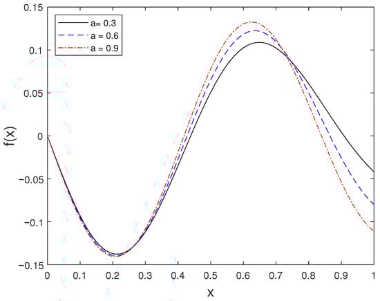
Figure 1. Source profile $f\left(x\right)$ for several values of a.

The numerical solution $U(x,t)$ computed at $a=0.3$ for several time levels is shown in Figure 2. This figure highlights the temporal evolution of the solution and confirms the stability of the reconstruction for a fixed value of a.

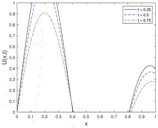
Figure 2. Solution $U(x,t)$ computed at $a=0.3$ for selected time levels t.

Figure 3 presents the solution $U(x,t)$ at the fixed time $t=0.1$ for different values of a. The comparison demonstrates the sensitivity of the solution profile with respect to changes in the parameter a.

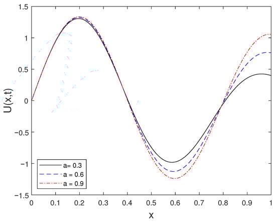
Figure 3. Solution $U(x,t)$ at $t=0.1$ for different a values.

The time dependent behavior of the solution $U(x,t)$ for $a=0.3$ is illustrated in Figure 4. As time increases, the figure shows the propagation characteristics of the wave under the imposed nonlocal boundary condition.

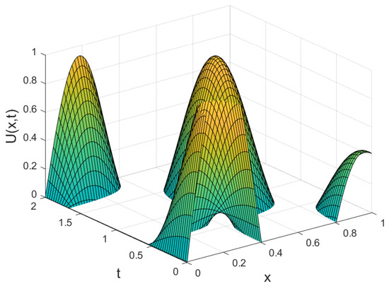
Figure 4. Behavior of $U(x,t)$ at $a=0.3$ as time increases.

6.2. Example

For the numerical illustration related to ISP II, we take

$$\psi \left(x\right)={\displaystyle \frac{sin\left({\sigma }_{j1}x\right)}{5!+T}},j=1,2,n=1,\rho \left(x\right)=1,F(x,t)=0.$$

By applying the spectral expansion technique, the coefficients become

$${\psi }_{20}=F_{20}\left(t\right)=0,{\psi }_{j1}={\displaystyle \frac{1}{5!+T}},F_{j1}\left(t\right)=0.$$

Similarly, the coefficients of $\rho \left(x\right)$ are given as follows:

$$\begin{array}{cc}\hfill {\rho }_{11}=& {\displaystyle \frac{-d_{11}}{{\sigma }_{11}}}(cos\left({\sigma }_{11}\alpha \right)-{\displaystyle \frac{cos\left({\sigma }_{11}\alpha \right)}{2cos\left({\sigma }_{11}(1-\alpha /2)\right)}}(cos\left({\sigma }_{11}\alpha \right)-cos\left({\sigma }_{11}\right)\hfill \\ \hfill +& tan\left({\sigma }_{11}\right)\left(sin\left({\sigma }_{11}\right)-sin\left({\sigma }_{11}\alpha \right)\right)\left)\right),\hfill \\ \hfill {\rho }_{21}=& {\displaystyle \frac{-c_2}{{\sigma }_{21}}}\left(cos\left({\sigma }_{21}\right)-cos\left({\sigma }_{21}\alpha \right)-tan\left({\sigma }_{21}\right)\left(sin\left({\sigma }_{21}\right)-sin\left({\sigma }_{21}\alpha \right)\right)\right),{\rho }_{20}=0.\hfill \end{array}$$

Consequently, the coefficients of $\varphi \left(x\right)$ are given by

$$\begin{array}{cc}\hfill {\varphi }_{11}=& {\displaystyle \frac{1}{cos\left(\sqrt{{\sigma }_{11}}T\right)}}\left({\displaystyle \frac{d_{11}}{{\sigma }_{11}}}\right(cos\left({\sigma }_{11}\alpha \right)-1-{\displaystyle \frac{cos\left({\sigma }_{11}\alpha \right)}{2cos\left({\sigma }_{11}(1-\alpha /2)\right)}}(cos\left({\sigma }_{11}\alpha \right)\hfill \\ \hfill -& cos\left({\sigma }_{11}\right)+tan\left(sin\left({\sigma }_{11}\right)-sin\left({\sigma }_{11}\alpha \right)\right)\left)\right)+{\displaystyle \frac{\sqrt{{\sigma }_{11}}sin\left(\sqrt{{\sigma }_{11}}T\right)}{5!+T}}),\hfill \end{array}$$

and

$$\begin{array}{cc}\hfill {\varphi }_{21}=& {\displaystyle \frac{-1}{cos\left(\sqrt{{\sigma }_{21}}T\right)}}\left({\displaystyle \frac{c_2}{{\sigma }_{21}}}\right(cos\left({\sigma }_{21}\right)-cos\left({\sigma }_{21}\alpha \right)-tan\left({\sigma }_{21}\right)(sin\left({\sigma }_{21}\right)\hfill \\ \hfill -& sin\left({\sigma }_{21}\alpha \right)\left)\right)-{\displaystyle \frac{\sqrt{{\sigma }_{21}}sin\left(\sqrt{{\sigma }_{21}}T\right)}{5!+T}}),\hfill \end{array}$$

${\varphi }_{20}=0,$ and the $U_{11}$, $U_{21}\left(t\right)$ and $U_{20}\left(t\right)$ are given by

$$U_{11}\left(t\right)={\rho }_{11}+{\displaystyle \frac{\sqrt{{\sigma }_{11}}sin\left(\sqrt{{\sigma }_{11}}t\right)}{5!+T}},and{U}_{21}\left(t\right)={\rho }_{21}+{\displaystyle \frac{\sqrt{{\sigma }_{21}}sin\left(\sqrt{{\sigma }_{21}}t\right)}{5!+T}}.$$

For ISP-II, the reconstructed initial condition $\varphi \left(x\right)$ for several values of a is plotted in Figure 5. The figure confirms that the recovered initial data is consistent with the imposed final condition.

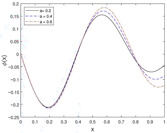
Figure 5. Source function $\varphi \left(x\right)$ plotted for several values of a.

The numerical solution $U(x,t)$ at $a=0.8$ for selected time instances is depicted in Figure 6. This figure demonstrates the effect of time evolution on the reconstructed solution for ISP-II.

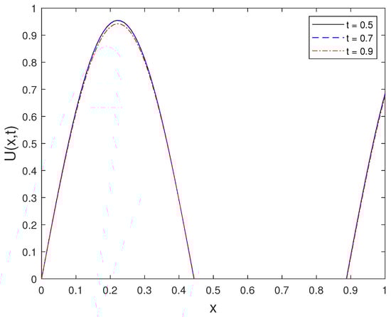
Figure 6. Numerical solution $U(x,t)$ at $a=0.8$ for selected times t.

Figure 7 shows the solution $U(x,t)$ at $t=0.1$ for different values of a. The results emphasize the influence of the parameter a on the spatial behavior of the solution.

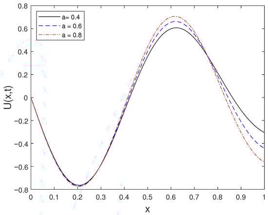
Figure 7. Solution $U(x,t)$ at $t=0.1$ for different values of a.

The evolution of the solution $U(x,t)$ for the fixed value $a=0.3$ is illustrated in Figure 8. This figure provides additional insight into the dynamic response of the system for ISP-II.

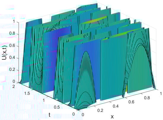
Figure 8. Solution $U(x,t)$ for $a=0.3$.

6.3. Example

For ISP-III, let the function $f(x,t)$ be defined as

$$f(x,t)=\sum _{j=1}^2\left({\displaystyle \frac{2}{t^2}}+{\sigma }_{j1}\right)sin\left({\sigma }_{j1}x\right),n=1,j=1,2.$$

Assume the initial condition in (2) and boundary conditions in (3) are zero. The additional integral condition takes the form

$${\int }_0^{1}U(x,t)dx=E\left(t\right)=\sum _{j=1}^2{\displaystyle \frac{-t^2}{{\sigma }_{j1}}}(cos{\sigma }_{j1}-1).$$

For $n=1$, we get the following solution

$$U(x,t)=\sum _{j=1}^2\left(a\left(t\right)f_{j1}\left(t\right)\ast \sqrt{{\sigma }_{j1}}sin\left(\sqrt{{\sigma }_{j1}}t\right)\right)X_{j1}\left(x\right),$$

where

$$f_{j1}\left(t\right)=\sum _{j=1}^2\left({\displaystyle \frac{2}{t^2}}+{\sigma }_{j1}\right).$$

For the term occurring in (48), then we obtain the following expression

$$\begin{array}{ccc}\hfill {\int }_0^{1}f(x,t)dx& =& \sum _{j=1}^2{\displaystyle \frac{-1}{{\sigma }_{j1}}}\left({\displaystyle \frac{2}{t^2}}+{\sigma }_{j1}\right)(cos{\sigma }_{j1}-1),E^{″}\left(t\right)=\sum _{j=1}^2{\displaystyle \frac{-2}{{\sigma }_{j1}}}(cos{\sigma }_{j1}-1),\hfill \\ \hfill \mathcal{F}\left(t\right)& =& 0,\mathcal{K}(t,\tau )=\sum _{j=1}^2{t}^2{\sigma }_{j1}(cos{\sigma }_{j1}-1).\hfill \end{array}$$

In this case, we can consider the expression of $a\left(t\right)$ that is

$$a\left(t\right)=2t^2.$$

Hence, we obtain

$$U(x,t)=\sum _{j=1}^2{t}^{2}sin\left({\sigma }_{j1}x\right).$$

For ISP-III, the reconstructed time dependent source term $a\left(t\right)$ for different powers of t is presented in Figure 9. This figure confirms the analytical expression obtained for $a\left(t\right)$ and validates the reconstruction procedure.

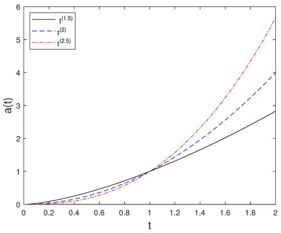
Figure 9. Source term $a\left(t\right)$ for several powers of t.

Finally, Figure 10 displays the numerical solution $U(x,t)$ corresponding to different time values. The figure illustrates the growth behavior of the solution and highlights the instability characteristics discussed in the theoretical analysis.

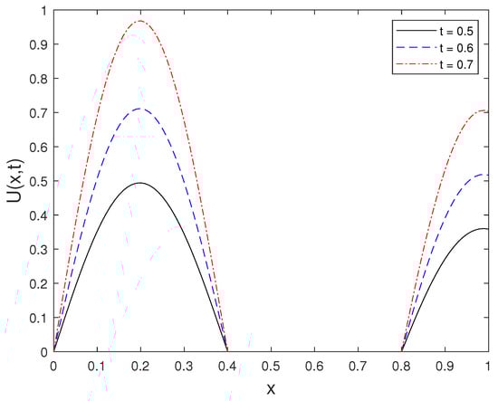
Figure 10. Numerical solution $U(x,t)$ for different values of t.

6.4. Numerical Example with Noisy Data

In this subsection, we construct a numerical example featuring noisy data. The final data $E\left(t\right)$ in Example Section 6.3 is intentionally perturbed to generate the resulting noisy data $\tilde{E}\left(t\right)$. The solution $a\left(t\right)$ is assessed using the final data $E\left(t\right)$, while the function derived from the noisy or perturbed data $\tilde{E}\left(t\right)$ is denoted as $\tilde{a}\left(t\right)$. Graphs illustrating the solution are generated for various orders of t at the time $T=1$. Figure 11 displays the plot of $E\left(t\right)$ alongside the noisy data $\tilde{E}\left(t\right)$. Figure 12 depicts the plot of the perturbed solution at $t=0.3$, while Figure 13 illustrates the perturbed solutions at $t=0.6$. Additionally, the plot at $t=0.9$ is shown in Figure 14. Outputs corresponding to noisy data are represented by dashed lines, while plots with solid lines depict solutions without noise.

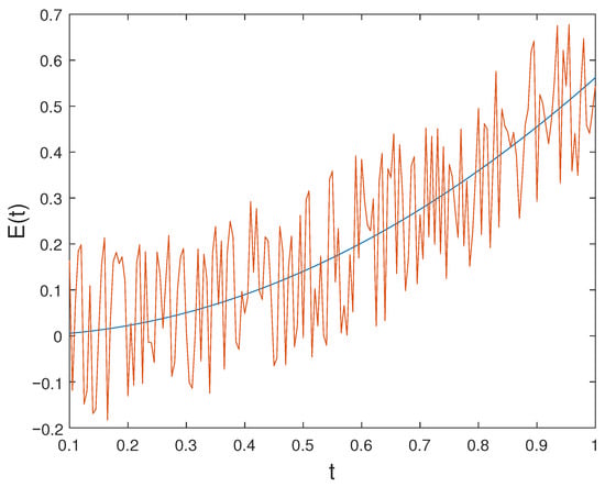
Figure 11. Exact data $E\left(t\right)$ and noisy observations $\tilde{E}\left(t\right)$.

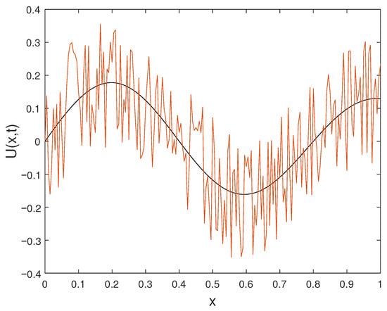
Figure 12. Exact solution $U(x,t)$ and noisy data $\tilde{U}(x,t)$ at $t=0.3$.

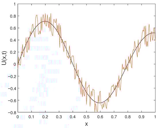
Figure 13. Exact and noisy solution profiles at $t=0.6$.

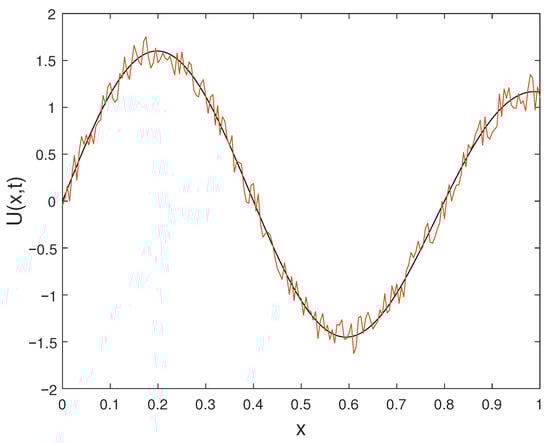
Figure 14. Exact and noisy solution profiles at $t=0.9$.

7. Conclusions

This study examined three ISPs associated with a wave equation subject to nonlocal boundary conditions. The solution methodology relied on series representations generated from a bi-orthogonal eigenfunction system. In the first problem, the spatial source term $f\left(x\right)$ was reconstructed by employing a final-time observation together with the state function $U(x,t)$, and existence and uniqueness were established under suitable regularity assumptions. In the second problem, the initial profile $\varphi \left(x\right)$ was recovered by using overspecified data at time T, and a unique regular solution was confirmed. In the third problem, the Banach fixed-point theorem was used to determine a time-dependent source function $a\left(t\right)$, ensuring the existence and uniqueness of the solution. Numerical experiments were provided for all three inverse problems to validate the theoretical findings.

References

- Chitorkin, E.E.; Bondarenko, N.P. Inverse Sturm-Liouville problem with polynomials in the boundary condition and multiple eigenvalues. J. Inv. Ill-Posed Prob. 2025, 33, 319–338. [Google Scholar] [CrossRef]
- Engl, H.W.; Groetsch, C.W. Inverse and Ill-Posed Problems; Elsevier: Amsterdam, The Netherlands, 2014; Volume 4. [Google Scholar]
- Romanov, V.; Hasanov, A. Uniqueness and stability analysis of final data inverse source problems for evolution equations. J. Inv. Ill-Posed Prob. 2022, 30, 425–446. [Google Scholar] [CrossRef]
- Il’in, V.A. How to express basis conditions and conditions for the equiconvergence with trigonometric series of expansions related to non-self-adjoint differential operators. Comput. Math. Appl. 1997, 34, 641–647. [Google Scholar] [CrossRef]
- Ilyas, A.; Khalid, R.A.; Malik, S.A. Identifying temperature distribution and source term for generalized diffusion equation with arbitrary memory kernel. Math. Methods Appl. Sci. 2024, 47, 5894–5915. [Google Scholar] [CrossRef]
- Friedman, A. Inverse Problems in Wave Propagation; Springer: New York, NY, USA, 1997. [Google Scholar]
- Roy, D.N.G. Methods of Inverse Problems in Physics; CRC Press: Boca Raton, FL, USA, 1991. [Google Scholar]
- Zhdanov, M.S. Inverse Theory and Applications in Geophysics; Elsevier: Amsterdam, The Netherlands, 2015. [Google Scholar]
- Evans, L.C. Partial Differential Equations; American Mathematical Society: Providence, RI, USA, 2022. [Google Scholar]
- Bertero, M.; Boccacci, P.; De Mol, C. Introduction to Inverse Problems in Imaging; CRC Press: Boca Raton, FL, USA, 2021. [Google Scholar]
- Sadybekov, M.; Dildabek, G.; Ivanova, M. Direct and inverse problems for nonlocal heat equation with boundary conditions of periodic type. Bound. Value Probl. 2022, 2022, 53. [Google Scholar] [CrossRef]
- Bazhlekova, E. Regarding a Class of Nonlocal BVPs for the General Time-Fractional Diffusion Equation. Fractal Fract. 2025, 9, 613. [Google Scholar] [CrossRef]
- Ilyas, A.; Malik, S.A.; Suhaib, K. Existence and Uniqueness Results for Generalized Non-local Hallaire-Luikov Moisture Transfer Equation. Acta Appl. Math. 2025, 195, 9. [Google Scholar] [CrossRef]
- Wei, T.; Xu, J.; Yue, X. Identifying the Order and a Space Source Term in a Time Fractional Diffusion-Wave Equation. East Asian J. Appl. Math. 2026, 16, 168–203. [Google Scholar] [CrossRef]
- Huntul, M.J.; Tamsir, M.; Dhiman, N. Identification of time-dependent potential in a fourth-order pseudo-hyperbolic equation from additional measurement. Math. Methods Appl. Sci. 2022, 45, 5249–5266. [Google Scholar] [CrossRef]
- Kirane, M.; Sadybekov, M.A.; Sarsenbi, A.A. On an inverse problem of reconstructing a subdiffusion process from nonlocal data. Math. Methods Appl. Sci. 2019, 42, 2043–2052. [Google Scholar] [CrossRef]
- Kirane, M.; Al-Salti, N. Inverse problems for a nonlocal wave equation with an involution perturbation. J. Nonlinear Sci. Appl. 2016, 9, 1243–1251. [Google Scholar] [CrossRef]
- Ahmad, B.; Alsaedi, A.; Kirane, M.; Tapdigoglu, R.G. An inverse problem for space and time fractional evolution equations with an involution perturbation. Quaest. Math. 2017, 40, 151–160. [Google Scholar] [CrossRef]
- Samreen, A.; Ilyas, A.; Ould Beinane, S.A.; Mansoor, L.B.E. Identifying the Anomalous Diffusion Process and Source Term in a Space-Time Fractional Diffusion Equation With Sturm-Liouville Operator. Math. Meth. Appl. Sci. 2025, 48, 12749–12760. [Google Scholar] [CrossRef]
- Sadybekov, M.A.; Sarsenbi, A.M. Solution of fundamental spectral problems for all the boundary value problems for a first-order differential equation with a deviating argument. Uzbek Math. J. 2007, 3, 88–94. [Google Scholar]
- Sadybekov, M.A.; Sarsenbi, A.M. On notion of regularity of boundary value problems for a second order differential equation with deviating argument. Math. J. 2007, 7, 18. [Google Scholar]
- Ruzhansky, M.; Tokmagambetov, N.; Torebek, B.T. Inverse source problems for positive operators I: Hypoelliptic diffusion and subdiffusion equations. J. Inverse Ill-Posed Probl. 2019, 27, 891–911. [Google Scholar] [CrossRef]
- Wiener, J.; Aftabizadeh, A.R. Boundary value problems for differential equations with reflection of the argument. Int. J. Math. Math. Sci. 1985, 8, 151–163. [Google Scholar] [CrossRef]
- Burlutskaya, M.S. Mixed problem for a first-order partial differential equation with involution and periodic boundary conditions. Comput. Math. Math. Phys. 2014, 54, 1–10. [Google Scholar] [CrossRef]
- Gupta, C.P. Existence and uniqueness theorems for boundary value problems involving reflection of the argument. Nonlinear Anal. Theory Methods Appl. 1987, 11, 1075–1083. [Google Scholar] [CrossRef]
- Lomov, I.S. Construction of a generalized solution of a mixed problem for the telegraph equation: Sequential and axiomatic approaches. Differ. Equ. 2022, 58, 1468–1481. [Google Scholar] [CrossRef]
- Podlubny, I. Fractional Differential Equations; Academic Press: San Diego, CA, USA, 1999. [Google Scholar]
- Podlubny, I. Fractional Differential Equations; Elsevier: Amsterdam, The Netherlands, 1998. [Google Scholar]
Disclaimer/Publisher’s Note: The statements, opinions and data contained in all publications are solely those of the individual author(s) and contributor(s) and not of MDPI and/or the editor(s). MDPI and/or the editor(s) disclaim responsibility for any injury to people or property resulting from any ideas, methods, instructions or products referred to in the content. |
© 2025 by the authors. Licensee MDPI, Basel, Switzerland. This article is an open access article distributed under the terms and conditions of the Creative Commons Attribution (CC BY) license (https://creativecommons.org/licenses/by/4.0/).