Two-Stage Analysis for Supply Chain Disruptions Considering the Trade-Off Between Profit Maximization and Adaptability

Abstract

Considering the trade-off between profit maximization and adaptability to supply chain disruptions, we examine herein the decision-making for configuration and distribution plans in a supply chain. Supply chain disruptions are caused by facility accidents and disasters. In this work, we investigate an optimal configuration and distribution plan in the supply chain with disruptions, including the opening of additional facilities while maintaining the optimum supply amounts to customers in the profit maximization plan when no such disruptions occur. Assuming the existence of uncertainties in demands and supplies, we formulate a two-stage model with a simple recourse, in which decisions on the supply chain configuration are made at the first stage. Decisions on the distribution are made at the second stage after the demands and supplies are realized. For such a configuration and distribution in the supply chain, we propose TSA-SCD (Two-Stage Analysis for Supply Chain Disruptions), a novel decision-making framework considering the trade-off between profit maximization and adaptability to supply chain disruptions. Accordingly, we perform numerical experiments with different degrees of disruptions to verify the effectiveness of the proposed decision method.

1. Introduction

When investigating the designs, operations, and management of supply chains considering the disruptions caused by facility accidents and disasters, we should also consider the trade-off between profit maximization or cost minimization and adaptability to supply chain disruptions. In this study, we evaluate supply chain management from two key criteria: profit maximization and adaptability to supply chain disruptions. These two criteria often conflict with each other, and balancing them is a critical issue for effective and resilient supply chain operations. Addressing this trade-off is the primary motivation of our research. Various aspects of evaluation criteria are considered for the designs, operations, and management of supply chains, and researchers investigate multiobjective decision problems in supply chains. This study focuses on maximizing the profit and adapting to supply chain disruptions.

During the 1980s and early 1990s, several fundamental methods for multiobjective decision-making were developed. Wierzbicki [1] introduced the reference point approach, while Ignizio [2] and Zeleny [3] provided systematic treatments of multiobjective optimization. Further methodological contributions were given by Chankong and Haimes [4], Sawaragi et al. [5], and Yu [6], who helped to disseminate the theoretical foundations of multiobjective decision-making. Subsequent works by Steuer [7], Seo and Sakawa [8], and Stadler [9] extended the field by presenting computational techniques and engineering applications. Haimes et al. [10] introduced hierarchical analysis for large-scale systems, and Sakawa [11] incorporated fuzzy set theory into interactive multiobjective optimization. Since the 1990s, research attention has increasingly turned toward supply chain management. Weber and Current [12] pioneered a multiobjective approach to vendor selection. Jayaraman [13] and Korpela et al. [14] applied multiobjective methods to logistics facility location and production capacity allocation in supply chains. Further studies by Erol and Ferrell Jr. [15,16] developed methodologies for selection and decision-making problems under multiple, conflicting objectives, while Zhou et al. [17] proposed a genetic algorithm for multiobjective customer-to-warehouse allocation. More recent contributions explicitly considered uncertainty and risk in supply chain design and supplier selection. Azaron et al. [18] proposed a stochastic programming approach to supply chain design under risk. Liao and Rittscher [19] developed a supplier selection model under stochastic demand conditions, and Demirtas and Ustun [20] presented an integrated multiobjective process for supplier selection and order allocation.

Looking back on the studies after 2010, Franca et al. [21] focused on two objectives, that is, maximizing the total profit of a supply chain and raising the quality level (i.e., minimizing the number of defects). They employed a two-stage model to deal with uncertainty and proposed a solution method using the $ϵ$-constraint method. Assuming that parameters such as demands can be represented by possibility distributions, Pishvaee and Torabi [22] formulated a fuzzy programming problem minimizing two objectives. The first objective is the total cost, including facility opening, transportation, and processing costs. The second one is the delivery delay time. They used an interactive method to find a satisfactory solution. Focusing on agrichemical supply chains, Liu and Papageorgiou [23] formulated a three-objective optimization problem, in which the total cost, weighted transportation time, and opportunity loss were minimized. They adopted the $ϵ$-constraint and minimax methods with the lexicographic order to obtain a satisfactory solution.

Huang and Goetschalckx [24] employed a two-stage model, in which the supply chain configuration is determined at the first stage, and the production and distribution are optimized at the second stage. They investigated the mean-standard deviation robust design problem, which is a type of two-objective problem formulated by subtracting $\kappa$ times the standard deviation from the expected return. They then developed a branch-and-reduce algorithm to solve the problem. Zhuang et al. [25] developed a two-stage stochastic programming approach with robust constraints for post-disruption logistics network design. Yang et al. [26] also used a two-stage model assuming joint possibility distributions for the transportation cost and demand and formulated a two-objective problem with the expected cost as a risk-neutral criterion and the weighted mean deviation as a risk-averse criterion. They found the Pareto front in the two-dimensional objective space by using a metaheuristic. Pasandideh et al. [27] dealt with a three-level supply chain consisting of factories, distribution centers, and customers and formulated a two-objective optimization problem with respect to the expected value and the total cost variance, assuming that the production and transportation costs, demand, and so on can be represented by normal probability distributions. They computed Pareto optimal solutions using NSGA-II and NRGA. Furthermore, approaches have been developed that integrate environmental impacts and profit objectives under both demand and supply uncertainty using multi-objective two-stage stochastic programming [28]. They computed Pareto optimal solutions using NSGA-II and NRGA.

Although the increasing investment in supply chain facilities promises greater resilience to disruptions, the total cost becomes larger. Supply chain managers must evaluate the trade-off between the ability to adapt to disruption risks in the supply chain and the corresponding cost. Nooraie and Parast [29] formulated a two-objective optimization problem, in which the total revenue is maximized, and the total cost, including the cost of opening facilities, is minimized to analyze the trade-off between the two objectives. The authors developed a decision-making model for the trade-off analysis between disruption mitigation by facility investments and profit and examined how much facility investment is justified in a supply chain with disruption risk. Given the scenarios of facility failures and uncertain demand, Refs. [30,31,32] also considered the cost minimization problem for opening reliable and unreliable facilities and product transportation.

In recent years, the growing attention to environmental issues, such as the reduction of greenhouse gas (GHG) emissions, has led to many studies on supply chain management considering the minimization of environmental impacts and the maximization of profit. Santibanez-Aguilar et al. [33] considered a two-objective stochastic programming problem with respect to profit and the environmental impacts in supply chain management for biorefineries, while Taghvaei et al. [34] developed a bi-objective two-stage stochastic programming model for resilient humanitarian relief supply chains under uncertainty. Assuming that the amount of biomass, fossil fuel production costs, and so on are uncertain parameters, Hombach et al. [35] modeled a sustainable supply chain by formulating a three-objective stochastic optimization problem. The first economic objective is the discounted net present value. The second environmental objective is the life cycle GHG emission. The third social objective is the land use change. Sawik [36] further addressed stochastic optimization of supply chain resilience under disruption risk. At the policy level, the need to strengthen supply chain resilience has also been highlighted internationally [37]. Nicoletti and You [38] investigated a two-level multiobjective programming problem, in which an oil refiner, as an upper-level decision-maker, considers the two objectives of profit and environmental impact, while an oil producer, as a lower-level decision-maker, aims to maximize profit. Karimi et al. [39] and Meng et al. [40] dealt with the supply chain of power generation using biomass and formulated a two-objective optimization problem of profit and GHG emission considering the uncertainty in the energy amount of biomass. In recent years, comprehensive reviews have also emerged from the inventory management perspective on supply chain resilience [41].

Based on our review of the abovementioned literature on supply chain management, many multiobjective problems under uncertainty from diverse perspectives have been investigated. Similar to the work of [29], we attempt herein to analyze the trade-off between profit maximization and adaptability to supply chain disruptions. Supply chain disruptions are assumed to be attributed to facility accidents and disasters. Recent case studies have shown that locally embedded supply chains can play a vital role during crises [42]. After obtaining the optimal configuration and distribution plan for the supply chain without any disruption, we consider an appropriate supply chain configuration, including opening additional facilities for the disrupted supply chain to maintain the optimal supply levels to customers, even during disruptions. We deal with a supply chain consisting of five layers: suppliers, factories, warehouses, distribution centers, and customers. Introducing external suppliers in addition to the usual suppliers, we also consider a multiperiod planning that considers product storage in warehouses and distribution centers.

Considering the multiperiod planning for a supply chain, we assume uncertainties in the amounts of supply and demand. We formulate a two-stage model, in which decisions on opening facilities are made at the first stage, and the distribution plan is determined at the second stage after the amounts of supply and demand are realized. From the standpoint of a supply chain manager, we develop a two-stage analysis approach for managing the supply chain that is prepared for disruptions while maximizing profit. After randomly sampled facilities become unavailable according to the specified degree of disruption, we solve the configuration and distribution planning problem for the supply chain. To eliminate bias in the computational result, unavailable facilities are randomly selected, and the problem is repeatedly solved. The same procedure is repeated after the degree of disruption is updated. Considering the trade-off between profit maximization and adaptability to supply chain disruptions, the supply chain manager finally chooses the appropriate degree of disruption and can obtain the preferable configuration and distribution plan for the supply chain with the anticipated disruption. We propose a two-stage analysis approach for configuration and distribution planning for the supply chain through a trade-off analysis by the supply chain manager.

The novelty of this paper is summarized as follows: First, we propose TSA-SCD (two-stage analysis for supply chain disruptions), a decision framework that jointly optimizes network configuration and multiperiod distribution while explicitly preparing for disruption levels chosen by the manager. Second, TSA-SCD integrates a two-stage (expectation/quantile) stochastic optimization model with Monte-Carlo disruption simulation, enabling quantitative trade-off analysis between profit and adaptability. Third, we provide actionable guidance on how the assured probability level $\theta$ (risk attitude) and the disruption degree $\mathrm{\Lambda }$ (preparedness) shape facility opening, inventory, and external sourcing decisions. Positioning with recent literature. Over the last decade, studies have advanced stochastic and robust models for supply chain design under uncertainty, as well as risk-aware formulations and disruption analytics. However, most approaches either optimize expected performance or adopt a single risk measure without offering a manager-driven mechanism to co-tune the disruption exposure and risk attitude within one optimization framework. By unifying an expectation model and a fractile (quantile) model under a service-preservation constraint, TSA-SCD fills this gap: it produces a profit–adaptability frontier indexed by disruption degree ($\mathrm{\Lambda }$) and risk attitude ($\theta$), and thus links modeling choices to actionable policies (facility openings, external contracting, and inventories) in a multi-echelon network. Our research question is how a supply chain manager can determine a configuration and distribution plan that balances profit maximization with adaptability to facility disruptions under joint demand–supply uncertainty.

In Section 2, we first revisit a representative two-objective formulation and clarify its limitations regarding explicit disruption representation. We then introduce TSA-SCD, which unifies an expectation model and a fractile (quantile) model under a service-preservation constraint to analyze the profit–adaptability trade-off transparently. Section 3 presents our numerical experiments to show the validity and effectiveness of the proposed decision method. Section 4 presents the concluding remarks.

2. Model

2.1. Formulation in Nooraie and Parast

In their study, Nooraie and Parast [29] considered the configuration of facilities (i.e., factories, warehouses, and distribution centers) and the distribution plan for a five-level supply chain consisting of suppliers, factories, warehouses, distribution centers, and customers. Assuming that parameters, such as prices and demands, are discrete random variables, they dealt with the two-objective problem of maximizing total profit and minimizing total cost, including transportation and facility opening costs.

The first objective function to be maximized is the sum of the expected sales revenue of the products and the expected revenue from the opened facilities. The second objective function to be minimized is the sum of the expected transportation cost and the expected facility opening cost. The facility flow constraints, capacity constraints of the facilities, supply capacity constraints, and demand constraints are imposed for each scenario of uncertainty. The two objective functions are the expected values of income and cost, and the supply chain disruptions are not well represented in their formulation; hence, the disruption risk in the supply chain may not always be fully evaluated. In the numerical example given by Nooraie and Parast [29], the complexity is reduced by formulating the problem as a single-objective problem by simply defining the objective function as cost minus income. Specifically, their bi-objective model optimizes expected profit and expected cost across scenarios but does not include explicit scenario-wise facility failure states (e.g., binary availability shocks or capacity-loss constraints) nor a service-preservation requirement under disruptions. Consequently, feasibility losses and tail outcomes induced by facility outages cannot be examined within their formulation. Numerically analyzing the trade-off between the two objectives by solving such a single-objective problem is not necessarily easy. Furthermore, the numerical example only has one parameter set, and the computational result indicates that all facilities are opened. Unfortunately, it is difficult to say that the trade-off between disruption risk in the supply chain and total cost can be adequately analyzed with this computational experiment.

2.2. Model for Representing Supply Chain Disruptions

Similar to [29], in the proposed method TSA-SCD (two-stage analysis for supply chain disruptions), we deal with a five-level supply chain consisting of suppliers, factories, warehouses, distribution centers, and customers (Figure 1) to analyze the trade-off between profit maximization and adaptability to supply chain disruptions. Furthermore, we assume that the warehouses and distribution centers have inventory storage capacities, and uncertainties exist in supplies and demands. We also introduce external suppliers [43] to adapt to supply uncertainties and formulate a two-stage model with a simple recourse to represent the uncertainties in supplies and demands.

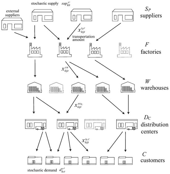
Figure 1. Supply Chain Model.

Let $S_P$, F, W, $D_C$, and C denote the sets of suppliers, factories, warehouses, distribution centers, and customers, respectively. Assume that a supply chain manager makes decisions about opening factories, warehouses, and distribution centers. Let $M=F\cup W\cup D_C$ be the set of facilities that the supply chain manager can open. Moreover, let K, T, and N be the set of products, periods, and external suppliers, respectively.

Let $S^S$ and $S^D$ be the sets of scenarios for supply and demand, respectively. We assume that the supply and demand depend on uncertain events and are represented by the following discrete random variables as shown in Equations (1) and (2), respectively:

$$\begin{array}{cc}\hfill & ((su{p}_{klt}^{s^s},{\pi }_s^{s^s}),s^s\in S^S),k\in K,l\in S_P,t\in T\hfill \end{array}$$

(1)

$$\begin{array}{cc}\hfill & ((d_{kct}^{s^d},{\pi }_d^{s^d}),s^d\in S^D),k\in K,c\in C,t\in T,\hfill \end{array}$$

(2)

where $su{p}_{klt}^{s^s}$ and $d_{kct}^{s^d}$ are the realized values of supply and demand at scenarios $s^s$th and $s^d$, respectively, and ${\pi }_s^{s^s}$ and ${\pi }_d^{s^d}$ are the corresponding occurrence probabilities.

The parameters and decision variables are defined below:

Parameters
$P{r}_{kct}$:	Unit price of product k for customer c in period t
$T{r}_{klit}^{S_{P}F}$:	Unit transportation cost of product k from supplier l to factory i in period t
$T{r}_{kijt}^{FW}$:	Unit transportation cost of product k from factory i to warehouse j in period t
$T{r}_{kijt}^{W{D}_C}$:	Unit transportation cost of product k from warehouse i to distribution center j in period t
$T{r}_{kict}^{D_{C}C}$:	Unit transportation cost of product k from distribution center i to customer c in period t
$C{o}_{it}$:	Opening cost of facility i in period t
$J_{nt}$:	Contract cost with external supplier n in period t
$V_{knt}$:	Supply capacity of product k of external supplier n in period t
$h_{kit}$:	Unit storage cost of product k in facility i in period t
$ca{p}_{kit}$:	Capacity for product k in facility i in period t
$su{p}_{klt}^{s^s}$:	Supply of product k from supplier l at scenario $s^s$ in period t
${\pi }^{s^s}$:	Probability that supply scenario $s^s$ occurs
$d_{kct}^{s^d}$:	Demand of product k for customer c at scenario $s^d$ in period t
${\pi }^{s^d}$:	Probability that demand scenario $s^d$ occurs
$P{e}_{klt+}^{S_P}$:	Penalty for undersupply of product k by supplier l in period t
$P{e}_{klt-}^{S_P}$:	Penalty for oversupply of product k by supplier l in period t
$P{e}_{kct+}^C$:	Penalty for undersupply of product k to customer c in period t
$P{e}_{kct-}^C$:	Penalty for oversupply of product k to customer c in period t

Decision variables
$x_{klit}^{S_{P}F}$:	Transportation amount of product k from supplier l to factory i in period t
$x_{kijt}^{FW}$:	Transportation amount of product k from factory i to warehouse j in period t
$x_{kijt}^{W{D}_C}$:	Transportation amount of product k from warehouse i to distribution center j in period t
$x_{kict}^{D_{C}C}$:	Transportation amount of product k from distribution center i to customer c in period t
$y_i$:	Open status of facility i (1 if open, otherwise 0)
$z_{nt}$:	Contract status with external supplier n in period t (1 if contracted, otherwise 0)
$I_{kit}$:	Inventory amount of product k in facility i in period t

Throughout Section 2, we use consistent subscripts: $l\in SP$ (suppliers), $i\in F$ (factories), $j\in W$ (warehouses), $m\in D_C$ (distribution centers), $c\in C$ (customers), $n\in N$, $k\in K$, and $t\in T$. Transportation variables follow the arc direction: $x_{klit}^{SPF}$ (SP→F), $x_{kijt}^{FW}$ (F→W), $x_{kjmt}^{W{D}_C}$ (W→DC), and $x_{kmct}^{D_{C}C}$ (DC→C).

Suppose that demand $d_{kct}^{s^d}$ at scenario $s^d$ is realized. ${\sum }_{i\in D_C}{x}_{kict}\ge d_{kct}^{s^d}$ implies an oversupply of product k to customer c in period t, and ${\sum }_{i\in D_C}{x}_{kict}\le d_{kct}^{s^d}$ depicts an undersupply of product k to customer c in period t, that is, there is residual demand. For any product $k\in K$, customer $c\in C$, period $t\in T$, introducing nonnegative variables ${\delta }_{kct+}^{s^d}$, ${\delta }_{kct-}^{s^d}$, $s^d\in S^D$, such that one of the two variables must be zero, we can describe the relationship between the supply amount of product k to customer c and the demand of customer c as Equation (3):

$$\sum _{i\in D_C}{x}_{kict}+{\delta }_{kct+}^{s^d}-{\delta }_{kct-}^{s^d}=d_{kct}^{s^d},s^d\in S^D,$$

(3)

where ${\delta }_{kct+}^{s^d}$ and ${\delta }_{kct-}^{s^d}$ represent the amounts of undersupply and oversupply, respectively, of product k to consumer c in period t.

The same applies to supply. For any product $k\in K$, supplier $l\in S_P$, period $t\in T$, introducing nonnegative variables ${\sigma }_{klt+}^{s^s}$, ${\sigma }_{klt-}^{s^s}$, $s^s\in S^S$, such that one of the two variables must be zero, we can describe the relationship between the supply amount $su{p}_{klt}^{s^s}$ of product k from supplier l and the transportation amount of product k from supplier l to all factories ${\sum }_{i\in F}{x}_{klit}^{S_{P}F}$ as Equation (4):

$$su{p}_{klt}^{s^s}+{\sigma }_{klt+}^{s^s}-{\sigma }_{klt-}^{s^s}=\sum _{i\in F}{x}_{klit}^{S_{P}F},s^s\in S^S,$$

(4)

where ${\sigma }_{klt+}^{s^s}$ and ${\sigma }_{klt-}^{s^s}$ represent the amounts of undersupply and oversupply, respectively, of product k by supplier l in period t. In case of an undersupply (i.e., ${\sigma }_{klt+}^{s^s}\ge 0$), the shortage of product k by supplier l in period t is provided by an external supplier. For example, when resolving the undersupply by supplier l by receiving the shortage from external supplier n, the following supply capacity constraint must be satisfied for any product $k\in K$ and period $t\in T$.

$${\sigma }_{klt+}^{s^s}\le \sum _{n\in N}{V}_{knt}{z}_{nt},s^s\in S^S.$$

(5)

2.2.1. Expectation Model

We consider the expectation model assuming that the supply chain manager is risk-neutral. The objective function of the expectation model is to maximize the expected profit calculated by subtracting the total cost comprising the transportation costs, facility opening costs, contract costs with external suppliers, storage costs in warehouses and distribution centers, and penalties for undersupply and oversupply at suppliers and consumers from the sales revenue from consumers. The penalties for the undersupply and oversupply are their expected values for all scenarios. We formulate the supply chain configuration and distribution planning problem in the expectation model as Equation (6):

$$\begin{array}{cc}\hfill \mathrm{maximize}& \sum _{k\in K}\sum _{c\in C}\sum _{t\in T}P{r}_{kct}\sum _{i\in D_C}{x}_{kijt}^{D_{C}C}-\sum _{k\in K}\sum _{t\in T}\left(\sum _{i\in S_P}\sum _{j\in F}T{r}_{kijt}^{S_{P}F}{x}_{kijt}^{S_{P}F}+\sum _{i\in F}\sum _{j\in W}T{r}_{kijt}^{FW}{x}_{kijt}^{FW}\right.\hfill \\ \hfill & \left.+\sum _{i\in W}\sum _{j\in D_C}T{r}_{kijt}^{W{D}_C}{x}_{kijt}^{W{D}_C}+\sum _{i\in D_C}\sum _{c\in C}T{r}_{kict}^{D_{C}C}{x}_{kict}^{D_{C}C}\right)-\sum _{i\in M}\sum _{t\in T}C{o}_{it}{y}_i-\sum _{n\in N}\sum _{t\in T}{J}_{nt}{z}_{nt}\hfill \\ \hfill & -\sum _{k\in K}\sum _{t\in T}\left(\sum _{i\in W}{h}_{kit}{I}_{kit}+\sum _{i\in D_C}{h}_{kit}{I}_{kit}\right)-\sum _{s^s\in S^S}{\pi }_s^{s^s}\sum _{k\in K}\sum _{l\in S_P}\sum _{t\in T}(P{e}_{klt+}^{S_P}{\sigma }_{klt+}^{s^s}+P{e}_{klt-}^{S_P}{\sigma }_{klt-}^{s^s})\hfill \end{array}$$

$$\begin{array}{cc}\hfill & -\sum _{s^d\in S^D}{\pi }_d^{s^d}\sum _{k\in K}\sum _{c\in C}\sum _{t\in T}(P{e}_{kct+}^C{\delta }_{kct+}^{s^d}+P{e}_{kct-}^C{\delta }_{kct-}^{s^d})\hfill \end{array}$$

(6a)

$$\begin{array}{cc}\hfill \mathrm{subject}\mathrm{to}& su{p}_{klt}^{s^s}+{\sigma }_{klt+}^{s^s}-{\sigma }_{klt-}^{s^s}=\sum _{j\in F}{x}_{kljt}^{S_{P}F},s^s\in S^S,k\in K,l\in S_P,t\in T\hfill \end{array}$$

(6b)

$$\begin{array}{cc}\hfill & \sum _{l\in S_P}{\sigma }_{klt+}^{s^s}\le \sum _{n\in N}{V}_{knt}{z}_{nt},s^s\in S^S,k\in K,t\in T\hfill \end{array}$$

(6c)

$$\begin{array}{cc}\hfill & \sum _{i\in S_P}{x}_{klmt}^{S_{P}F}=\sum _{j\in W}{x}_{kmjt}^{FW},k\in K,m\in F,t\in T\hfill \end{array}$$

(6d)

$$\begin{array}{cc}\hfill & \sum _{i\in S_P}{x}_{kljt}^{S_{P}F}\le ca{p}_{kjt}{y}_{jt},k\in K,j\in F,t\in T\hfill \end{array}$$

(6e)

$$\begin{array}{cc}\hfill & I_{kjt}=I_{kj(t-1)}+\sum _{i\in F}{x}_{kijt}^{FW}-\sum _{j\in D_C}{x}_{kjmt}^{W{D}_C},k\in K,m\in W,t\in T\hfill \end{array}$$

(6f)

$$\begin{array}{cc}\hfill & I_{km(t-1)}+\sum _{i\in F}{x}_{kimt}^{FW}\le ca{p}_{kmt}{y}_{mt},k\in K,m\in W,t\in T\hfill \end{array}$$

(6g)

$$\begin{array}{cc}\hfill & I_{kmt}=I_{km(t-1)}+\sum _{i\in W}{x}_{kimt}^{W{D}_C}-\sum _{c\in C}{x}_{kmct}^{D_{C}C},k\in K,m\in D_C,t\in T\hfill \end{array}$$

(6h)

$$\begin{array}{cc}\hfill & I_{km(t-1)}+\sum _{i\in W}{x}_{kimt}^{W{D}_C}\le ca{p}_{kmt}{y}_{mt},k\in K,m\in D_C,t\in T\hfill \end{array}$$

(6i)

$$\begin{array}{cc}\hfill & \sum _{i\in D_C}{x}_{kmct}^{D_{C}C}+{\delta }_{kct+}^{s^d}-{\delta }_{kct-}^{s^d}=d_{kct}^{s^d},s^d\in S^D,k\in K,c\in C,t\in T\hfill \end{array}$$

(6j)

$$\begin{array}{cc}\hfill & y_{it}\in \{0,1\},i\in M,t\in T\hfill \end{array}$$

(6k)

$$\begin{array}{cc}\hfill & z_{nt}\in \{0,1\},n\in N,t\in T\hfill \end{array}$$

(6l)

$$\begin{array}{cc}\hfill & x_{kljt}^{S_{P}F}\ge 0,x_{kijt}^{FW}\ge 0,x_{kijt}^{W{D}_C}\ge 0,x_{kict}^{D_{C}C}\ge 0,k\in K,l\in S_P,i,j\in M,c\in C,t\in T.\hfill \end{array}$$

(6m)

The first term of the objective function (6a) is sales revenue. The second term is all transportation costs from suppliers to customers. The third term is the opening cost of facilities. The fourth term is the contract cost with external suppliers. The fifth term is the inventory storage cost in warehouses and distribution centers. The sixth and seventh terms are the expected penalties for undersupply and oversupply, respectively, at suppliers and customers. Equation (6b) presents the constraint on uncertain supply, as described in (4). Inequality (6c) is a constraint on external suppliers, as described in (5). Equation (6d) is a flow constraint at factory m, which means that the amount of products shipped from all suppliers to factory m is equal to the amount of products shipped from factory m to all warehouses. Inequality (6e) is a capacity constraint for factory j. Equation (6f) is an inventory flow constraint at warehouse m. Inequality (6g) is a capacity constraint for warehouse m. Equation (6h) is an inventory flow constraint at distribution center m. Inequality (6i) is a capacity constraint for distribution center m. Equation (6j) is a constraint on uncertain demand, as described in (3).

2.2.2. Fractile Model

We employed the fractile model [44,45] to deal with the risk attitude of the supply chain manager, who is a decision maker for the profit maximization problem with uncertain supply and demand. We adopt Value at Risk (VaR) primarily for managerial interpretability and tactical decision transparency: it encodes an assured probability level $\mathrm{\theta }$ by maximizing a profit threshold f with $\mathbb{P}\{\mathrm{\Pi }(x,y)\ge f\}\ge \theta$ (cf. Equations (8) and (11)), under the service-preservation constraint (Equation (9)). While modern MILP solvers facilitate computation, our choice is driven by this assurance-based control of the lower tail of profit rather than implementation convenience [46,47,48,49,50,51].

Let us suppose that the supply chain manager maximizes the stochastic profit $\tilde{R}$. In the fractile model, the target variable f as a proxy for the stochastic profit $\tilde{R}$ is maximized under the condition that the probability that the profit $\tilde{R}$ is larger than or equal to the target variable f is larger than or equal to the assured probability level $\theta$ specified by the supply chain manager. The fractile model is formulated as (7):

$$\mathrm{maximize}f\mathrm{subject}\mathrm{to}P(\tilde{R}\ge f)\ge \theta .$$

(7)

The supply chain manager can obtain an effectual configuration and distribution plan for a supply chain according to his or her risk attitude by appropriately specifying the assured probability level $\theta$. That is, the supply chain manager can assess tail risk under the risk-averse preference or pursue a high profit potential under risk-prone preference.

In the fractile model (7), the supply chain manager specifies the assured probability level $\theta$ considering stochastically fluctuating profit and his or her own risk attitude. If the assured probability level $\theta$ is specified at a relatively large value, say 0.9, the supply chain manager can be interpreted as risk-averse because the profit level of the bottom 10% is maximized when $\theta =0.9$. Assuming that the realized profit is unfavorable, that is, if the profit is realized to be small (e.g., bottom 10% profit level), it is considered appropriate for the supply chain manager who wants to increase such a low profit level to set the assured probability level as $\theta =0.9$.

Conversely, if the assured probability level $\theta$ is a relatively small value, say 0.1, the supply chain manager can be interpreted as risk-prone because the profit level of the top 10% is maximized when $\theta =0.1$. Assuming that the realized profit is favorable, that is, if the profit level is realized to be large (e.g., top 10% profit level), it is considered appropriate for the supply chain manager who wants to increase such a high profit level to set the assured probability level as $\theta =0.1$. In this case, although the bottom profit levels may be quite small, it is considered appropriate for the supply chain manager who wants to maximize a high profit level.

The supply chain configuration and distribution problem is formulated according to the fractile model focusing on demand fluctuations, as shown in Equation (8):

$$\begin{array}{cc}\hfill \mathrm{maximize}& f\hfill \end{array}$$

(8a)

$$\begin{array}{cc}\hfill \mathrm{subject}\mathrm{to}& f-R^{s^d}\le \mathcal{M}{e}^{s^d},s^d\in S^D\hfill \end{array}$$

(8b)

$$\sum _{s^d\in S^D}{\pi }_d^{s^d}{e}^{s^d}\le 1-\theta$$

(8c)

$$\begin{array}{cc}\hfill & R^{s^d}=\sum _{k\in K}\sum _{c\in C}\sum _{t\in T}P{r}_{kct}\sum _{i\in D_C}{x}_{kijt}^{D_{C}C}-\sum _{k\in K}\sum _{t\in T}\left(\sum _{i\in S_P}\sum _{j\in F}T{r}_{kijt}^{S_{P}F}{x}_{kijt}^{S_{P}F}\right.\hfill \\ \hfill & \left.+\sum _{i\in F}\sum _{j\in W}T{r}_{kijt}^{FW}{x}_{kijt}^{FW}+\sum _{i\in W}\sum _{j\in D_C}T{r}_{kijt}^{W{D}_C}{x}_{kijt}^{W{D}_C}+\sum _{i\in D_C}\sum _{c\in C}T{r}_{kict}^{D_{C}C}{x}_{kict}^{D_{C}C}\right)\hfill \\ \hfill & -\sum _{i\in M}\sum _{t\in T}C{o}_{it}{y}_i-\sum _{n\in N}\sum _{t\in T}{J}_{nt}{z}_{nt}-\sum _{k\in K}\sum _{t\in T}\left(\sum _{i\in W}{h}_{kit}{I}_{kit}+\sum _{i\in D_C}{h}_{kit}{I}_{kit}\right)\hfill \\ \hfill & -\sum _{s^s\in S^S}{\pi }_s^{s^s}\sum _{k\in K}\sum _{l\in S_P}\sum _{t\in T}(P{e}_{klt+}^{S_P}{\sigma }_{klt+}^{s^s}+P{e}_{klt-}^{S_P}{\sigma }_{klt-}^{s^s})\hfill \end{array}$$

$$\begin{array}{cc}\hfill & -\sum _{k\in K}\sum _{c\in C}\sum _{t\in T}(P{e}_{kct+}^C{\delta }_{kct+}^{s^d}+P{e}_{kct-}^C{\delta }_{kct-}^{s^d})\hfill \end{array}$$

(8d)

$$\begin{array}{cc}\hfill & su{p}_{klt}^{s^s}+{\sigma }_{klt+}^{s^s}-{\sigma }_{klt-}^{s^s}=\sum _{j\in F}{x}_{kljt}^{S_{P}F},s^s\in S^S,k\in K,l\in S_P,t\in T\hfill \end{array}$$

(8e)

$$\begin{array}{cc}\hfill & \sum _{l\in S_P}{\sigma }_{klt+}^{s^s}\le \sum _{n\in N}{V}_{knt}{z}_{nt},s^s\in S^S,k\in K,t\in T\hfill \end{array}$$

(8f)

$$\begin{array}{cc}\hfill & \sum _{i\in S_P}{x}_{klmt}^{S_{P}F}=\sum _{j\in W}{x}_{kmjt}^{FW},k\in K,m\in F,t\in T\hfill \end{array}$$

(8g)

$$\begin{array}{cc}\hfill & \sum _{i\in S_P}{x}_{kljt}^{S_{P}F}\le ca{p}_{kjt}{y}_{jt},k\in K,j\in F,t\in T\hfill \end{array}$$

(8h)

$$\begin{array}{cc}\hfill & I_{kjt}=I_{kj(t-1)}+\sum _{i\in F}{x}_{kijt}^{FW}-\sum _{j\in DC}{x}_{kjmt}^{W{D}_C},k\in K,j\in W,t\in T\hfill \end{array}$$

(8i)

$$\begin{array}{cc}\hfill & I_{km(t-1)}+\sum _{i\in F}{x}_{kimt}^{FW}\le ca{p}_{kmt}{y}_{mt},k\in K,m\in W,t\in T\hfill \end{array}$$

(8j)

$$\begin{array}{cc}\hfill & I_{kmt}=I_{km(t-1)}+\sum _{i\in W}{x}_{kimt}^{W{D}_C}-\sum _{c\in C}{x}_{kmct}^{D_{C}C},k\in K,m\in D_C,t\in T\hfill \end{array}$$

(8k)

$$\begin{array}{cc}\hfill & I_{km(t-1)}+\sum _{i\in W}{x}_{kimt}^{W{D}_C}\le ca{p}_{kmt}{y}_{mt},k\in K,m\in D_C,t\in T\hfill \end{array}$$

(8l)

$$\begin{array}{cc}\hfill & \sum _{i\in D_C}{x}_{kmct}^{D_{C}C}+{\delta }_{kct+}^{s^d}-{\delta }_{kct-}^{s^d}=d_{kct}^{s^d},s^d\in S^D,k\in K,c\in C,t\in T\hfill \end{array}$$

(8m)

$$\begin{array}{cc}\hfill & y_{it}\in \{0,1\},i\in M,t\in T\hfill \end{array}$$

(8n)

$$\begin{array}{cc}\hfill & z_{nt}\in \{0,1\},n\in N,t\in T\hfill \end{array}$$

(8o)

$$\begin{array}{cc}\hfill & e^{s^d}\in \{0,1\},s^d\in S^D\hfill \\ \hfill & x_{kljt}^{S_{P}F}\ge 0,x_{kijt}^{FW}\ge 0,x_{kijt}^{W{D}_C}\ge 0,x_{kict}^{D_{C}C}\ge 0,\hfill \end{array}$$

(8p)

$$\begin{array}{cc}\hfill & k\in K,l\in S_P,i,j\in M,c\in C,t\in T\hfill \end{array}$$

(8q)

Equation (8d) presents the profit $R^{s^d}$ at demand scenario $s^d\in S^D$. It is the same as the objective function (6a) of the expectation model, except for the demand penalties. The objective function (8a) is the target variable f to be maximized as a proxy for the stochastic profit $\tilde{R}$. The fractile model is characterized by constraints (8b) and (8c). The supply chain manager specifies parameter $\theta \in (0,1)$. When $\theta$ is set close to 0, the supply chain manager expects as much profit as possible, despite the probability that the obtained large profit may be small. Conversely, setting $\theta$ close to 1 means that the supply chain manager wants to avoid extremely low profits.

In problem (8), we employed a formulation focusing on demand scenarios $s^d\in S^D$ because we handled the supply uncertainty by introducing external suppliers. However, we can also formulate a problem in which we deal with the profit depending on both the supply $s^s\in S^S$ and demand $s^d\in S^D$ scenarios. We will discuss this issue in Section 2.2.4.

2.2.3. Trade-Off Between Profit Maximization and Adaptability to Supply Chain Disruptions

In recent years, concerns about the vulnerability of supply chains have arisen due to the failures and shutdowns of facilities. We analyze the trade-off between profit maximization and adaptability to supply chain disruptions here. First, assuming no disruptions in the supply chain, we obtain an optimal supply chain configuration and distribution plan by solving problem (6) in the expectation model or problem (8) in the fractile model. The expectation model (6) provides a risk-neutral baseline that maximizes expected profit under uncertainty, while the fractile model (8) explicitly incorporates the decision maker’s risk attitude through the assured probability level $\theta$. By considering both formulations in parallel, our approach captures not only the average-case efficiency of the supply chain but also the robustness of decisions under unfavorable scenarios. This integration offers a more comprehensive decision-making framework compared with relying on either model alone. Next, we consider a situation in which some facilities in the supply chain have become unusable for some reason. We specify the degree of disruption indicating how many facilities are unavailable, identify these unavailable facilities, and remove them. Bias exists in unavailable facilities; hence, we use simulation techniques to find the average performance by repeatedly solving problem (6) or (8). We develop a supply chain configuration and distribution plan under the specified degree of disruption, maintaining the supply levels to the customers in the optimal plan obtained by solving problem (6) or (8).

Let ${\sum }_{i\in D_C}{x}_{kict}^{\ast D_{C}C}$ be the optimal transportation amount to customer c in problem (6) or (8). By adding constraints

$$\sum _{i\in D_C}{x}_{kict}^{D_{C}C}\ge \sum _{i\in D_C}{x}_{kict}^{\ast D_{C}C},k\in K,t\in T,c\in C$$

(9)

to problem (6) or (8) where the number of available facilities is reduced according to the specified degree of disruption, we can formulate the problem maximizing the profit of the supply chain under disruptions, maintaining the supply levels when no disruption exists. The degree of disruption $\mathrm{\Lambda }$ is defined as the unusable ratio (%) among all facilities.

The procedure of the TSA-SCD framework considering the trade-off between profit maximization and adaptability to supply chain disruptions is as follows:

Step 1: 

Solve problem (6) or (8) such that all facilities are available.

Step 2: 

The supply chain manager specifies a step size $\lambda$ and the maximum degree of disruption ${\mathrm{\Lambda }}_{max}$. Initialize the degree of disruption as $\mathrm{\Lambda }=\lambda$.

Step 3: 

For the degree of disruption $\mathrm{\Lambda }$, randomly choose facilities that cannot be used and remove them.

Step 4: 

Solve problem (6) or (8) such that constraint (9) is added to maintain the supply levels without disruption obtained in Step 1.

Step 5: 

If the problem solved in Step 4 is infeasible, increase the number of facilities that can be opened until it becomes feasible. The facility opening costs at the time of expansion are set higher than the normal costs.

Step 6: 

If the number of iterations specified in advance is reached, calculate the average values of the profit, costs, etc. Go to Step 7; otherwise, return to Step 3.

Step 7: 

If the degree of disruption $\mathrm{\Lambda }$ reaches the maximum degree ${\mathrm{\Lambda }}_{max}$, go to Step 8; otherwise, increment the degree $\mathrm{\Lambda }$ of disruption (i.e., $\mathrm{\Lambda }=\mathrm{\Lambda }+\lambda$), and then return to Step 3.

Step 8: 

The supply chain manager compares the solutions obtained so far and chooses a satisfactory solution considering the trade-off between profit maximization and adaptability to supply chain disruptions. Terminate the procedure.

Figure 2 summarizes the TSA-SCD workflow in an Inputs → Process → Outputs format, corresponding to Steps 1–8.

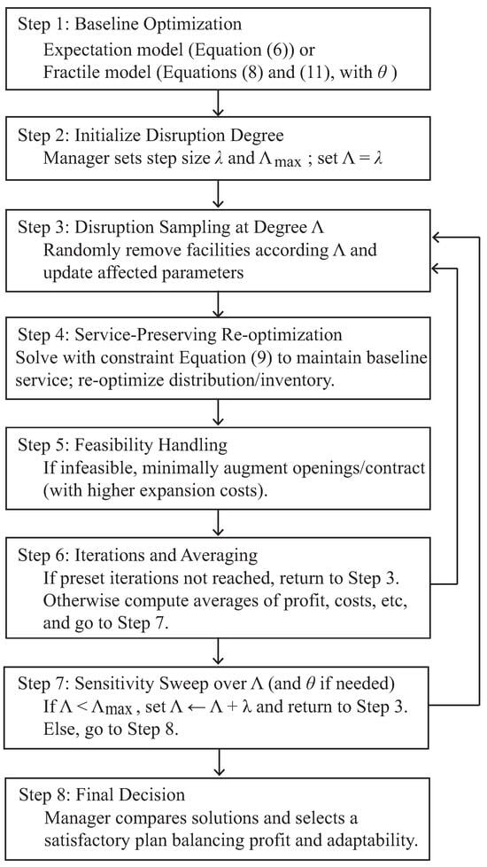
Figure 2. Workflow of TSA-SCD.

TSA-SCD is optimization-centric rather than score-based MCDM. While methods such as AHP, TOPSIS, BWM, ANP, DEMATEL, or VIKOR can support preference elicitation and ex-post ranking, the core engine here is a two-stage stochastic network design with simple recourse that (i) preserves baseline service at an explicit disruption degree via Equation (9) and (ii) controls the lower tail of profit through the fractile model in Equations (8) and (11). MCDM techniques are complementary in three places: before optimization, to elicit managerial preferences and map them into $(\mathrm{\Lambda },\theta )$ and penalty ratios; during model calibration, to prioritize disruption patterns or regions in the biased sampling of Section 2.2.4; and after optimization, to rank a small set of candidate plans using multiple KPIs (e.g., profit mean/variance, added capacity, utilization). In contrast to pure MCDM scoring, TSA-SCD enforces network feasibility, capacity, flow conservation, and inventory dynamics explicitly.

In Step 1, the optimal plan is obtained when no disruption exists in the supply chain. We make certain facilities unavailable in Step 3; thus, by repeating steps 3 to 6, we can obtain the average performance of the optimal plans for all trials with respect to the specified degree of disruption $\mathrm{\Lambda }$. In Step 8, after evaluating the trade-off between profit maximization and adaptability to supply chain disruptions based on the preference of the supply chain manager, the manager finally chooses a satisfactory solution. The supply chain manager can then obtain a supply chain configuration and distribution plan consistent with his or her preference. In the case of the fractile model, the abovementioned procedure is performed for each assured probability level $\theta$.

We adopt a tactical two-stage design in which facility openings and external contracts are first-stage decisions fixed over the planning horizon, whereas distribution and inventories are recourse decisions that adapt to realized demand/supply and simulated disruptions. Allowing period-by-period (re)opening would require a multistage dynamic model; such extensions (e.g., SDDP or the progressive hedging algorithm) are left for future work due to data and computational considerations. Within this tactical scope, Step 5 in Section 2.2.3 restores feasibility under disruptions by minimally augmenting openings/contracts with higher expansion costs, rather than re-optimizing (re)openings every period.

The procedure enables the supply chain manager to make decisions on the supply chain configuration and distribution planning considering the supply chain disruptions. For example, when the degree of disruption is $\mathrm{\Lambda }$, $\mathrm{\Lambda }\%$ of the total available facilities becomes unusable for some reasons. The profit is then maximized under this situation. For the degree of disruption $\mathrm{\Lambda }$, the supply chain manager should consider planning for more or less disruption. In the proposed procedure, after the supply chain manager evaluates the optimal plans for situations corresponding to all the degrees of disruption to determine how much to sacrifice the decrease in the profit to deal with supply chain disruptions, the manager finally decides what level of disruption to assume.

2.2.4. Discussion

Assuming that the supply uncertainty is mitigated by introducing external suppliers, we formulated the fractile model (8) in Section 2.2.2 focusing only on demand uncertainty. Although this formulation can reduce the number of scenarios generated from the discrete probability distribution, it is important to consider the uncertainty of supply and demand at the same time. Here, we take the fractile model complying with the joint probability distributions of supply and demand.

We assume that the amounts of supply and demand depend on uncertain events and are represented by the following discrete random variables:

$$((su{p}_{klt}^{s^{sd}},d_{kct}^{s^{sd}},{\pi }^{s^{sd}}),s^{sd}\in S^{SD}),k\in K,l\in S_P,c\in C,t\in T,$$

(10)

where $su{p}_{klt}^{s^{sd}}$ and $d_{kct}^{s^{sd}}$ are the realized values of supply and demand, respectively, at scenario $s^{s^{sd}}$, and ${\pi }^{s^{sd}}$ is the corresponding occurrence probability. $S^{SD}$ is a set of scenarios, and $s^{sd}$ is an index of a scenario.

The fractile model complying with the joint probability distribution of supply and demand is formulated as follows, as shown in Equation (11):

$$\begin{array}{cc}\hfill \mathrm{maximize}& f\hfill \end{array}$$

(11a)

$$\begin{array}{cc}\hfill \mathrm{subject}\mathrm{to}& f-R^{s^{sd}}\le \mathcal{M}{e}^{s^{sd}},s^{sd}\in S^{SD}\hfill \end{array}$$

(11b)

$$\sum _{s^d\in S^{sd}}{\pi }^{s^{sd}}{e}^{s^{sd}}\le 1-\theta$$

(11c)

$$\begin{array}{cc}\hfill & R^{s^{sd}}=\sum _{k\in K}\sum _{c\in C}\sum _{t\in T}P{r}_{kct}\sum _{i\in D_C}{x}_{kijt}^{D_{C}C}-\sum _{k\in K}\sum _{t\in T}\left(\sum _{i\in S_P}\sum _{j\in F}T{r}_{kijt}^{S_{P}F}{x}_{kijt}^{S_{P}F}+\sum _{i\in F}\sum _{j\in W}T{r}_{kijt}^{FW}{x}_{kijt}^{FW}\right.\hfill \\ \hfill & \left.+\sum _{i\in W}\sum _{j\in D_C}T{r}_{kijt}^{W{D}_C}{x}_{kijt}^{W{D}_C}+\sum _{i\in D_C}\sum _{c\in C}T{r}_{kict}^{D_{C}C}{x}_{kict}^{D_{C}C}\right)-\sum _{i\in M}\sum _{t\in T}C{o}_{it}{y}_i-\sum _{n\in N}\sum _{t\in T}{J}_{nt}{z}_{nt}\hfill \\ \hfill & -\sum _{k\in K}\sum _{t\in T}\left(\sum _{i\in W}{h}_{kit}{I}_{kit}+\sum _{i\in D_C}{h}_{kit}{I}_{kit}\right)-\sum _{k\in K}\sum _{l\in S_P}\sum _{t\in T}(P{e}_{klt+}^{S_P}{\sigma }_{klt+}^{s^{sd}}+P{e}_{klt-}^{S_P}{\sigma }_{klt-}^{s^{sd}})\hfill \end{array}$$

$$\begin{array}{cc}\hfill & -\sum _{k\in K}\sum _{c\in C}\sum _{t\in T}(P{e}_{kct+}^C{\delta }_{kct+}^{s^{sd}}+P{e}_{kct-}^C{\delta }_{kct-}^{s^{sd}})\hfill \end{array}$$

(11d)

$$\begin{array}{cc}\hfill & su{p}_{klt}^{s^{sd}}+{\sigma }_{klt+}^{s^{sd}}-{\sigma }_{klt-}^{s^{sd}}=\sum _{j\in F}{x}_{kljt}^{S_{P}F},s^{sd}\in S^{SD},k\in K,l\in S_P,t\in T\hfill \end{array}$$

(11e)

$$\begin{array}{cc}\hfill & \sum _{l\in S_P}{\sigma }_{klt+}^{s^{sd}}\le \sum _{n\in N}{V}_{knt}{z}_{nt},s^{sd}\in S^{SD},k\in K,t\in T\hfill \end{array}$$

(11f)

$$\begin{array}{cc}\hfill & \sum _{i\in S_P}{x}_{klmt}^{S_{P}F}=\sum _{j\in W}{x}_{kmjt}^{FW},k\in K,m\in F,t\in T\hfill \end{array}$$

(11g)

$$\begin{array}{cc}\hfill & \sum _{i\in S_P}{x}_{kljt}^{S_{P}F}\le ca{p}_{kjt}{y}_{jt},k\in K,j\in F,t\in T\hfill \end{array}$$

(11h)

$$\begin{array}{cc}\hfill & I_{kjt}=I_{kj(t-1)}+\sum _{i\in F}{x}_{kijt}^{FW}-\sum _{m\in DC}{x}_{kjmt}^{W{D}_C},k\in K,j\in W,t\in T\hfill \end{array}$$

(11i)

$$\begin{array}{cc}\hfill & I_{km(t-1)}+\sum _{i\in F}{x}_{kimt}^{FW}\le ca{p}_{kmt}{y}_{mt},k\in K,m\in W,t\in T\hfill \end{array}$$

(11j)

$$\begin{array}{cc}\hfill & I_{kmt}=I_{km(t-1)}+\sum _{i\in W}{x}_{kimt}^{W{D}_C}-\sum _{c\in C}{x}_{kmct}^{D_{C}C},k\in K,m\in D_C,t\in T\hfill \end{array}$$

(11k)

$$\begin{array}{cc}\hfill & I_{km(t-1)}+\sum _{i\in W}{x}_{kimt}^{W{D}_C}\le ca{p}_{kmt}{y}_{mt},k\in K,m\in D_C,t\in T\hfill \end{array}$$

(11l)

$$\begin{array}{cc}\hfill & \sum _{i\in D_C}{x}_{kmct}^{D_{C}C}+{\delta }_{kct+}^{s^{sd}}-{\delta }_{kct-}^{s^{sd}}=d_{kct}^{s^{sd}},s^{sd}\in S^{SD},k\in K,c\in C,t\in T\hfill \end{array}$$

(11m)

$$\begin{array}{cc}\hfill & y_{it}\in \{0,1\},i\in M,t\in T\hfill \end{array}$$

(11n)

$$\begin{array}{cc}\hfill & z_{nt}\in \{0,1\},n\in N,t\in T\hfill \end{array}$$

(11o)

$$\begin{array}{cc}\hfill & e^{s^{sd}}\in \{0,1\},s^{sd}\in S^{SD}\hfill \end{array}$$

(11p)

$$\begin{array}{cc}\hfill & x_{kljt}^{S_{P}F}\ge 0,x_{kijt}^{FW}\ge 0,x_{kijt}^{W{D}_C}\ge 0,x_{kict}^{D_{C}C}\ge 0,k\in K,l\in S_P,i,j\in M,c\in C,t\in T\hfill \end{array}$$

(11q)

The fractile model adopts VaR because it directly encodes a manager-specified assured probability level $\theta$ by maximizing a profit threshold f such that $\mathbb{P}\{\mathrm{\Pi }(x,y)\ge f\}\ge \theta$ (cf. Equations (8) and (11))), under the service-preservation constraint (Equation (9)). This yields an interpretable assurance on the lower tail of profit and a transparent mapping from $(\mathrm{\Lambda },\theta )$ to service-preserving policies. Conditional Value-at-Risk (CVaR), which controls the average loss beyond the VaR quantile, is also suitable when tail-average performance is emphasized; it can replace the objective in our TSA-SCD with no change to the feasibility constraints (see, e.g., [49]). Let ${\ell }_s=-{\mathrm{\Pi }}_s(x,y)$ denote scenario loss and $\alpha \in (0,1)$. A standard ${\mathrm{CVaR}}_{\alpha }$ objective is

$$\underset{x,y,\eta ,\left\{{\xi }_s\right\}}{min}\eta +{\displaystyle \frac{1}{(1-\alpha )\left|\mathcal{S}\right|}}\sum _{s\in \mathcal{S}}{\xi }_s\mathrm{s}.\mathrm{t}.{\xi }_s\ge {\ell }_s(x,y)-\eta ,{\xi }_s\ge 0,$$

together with Equation (9), Equation (6) (or Equations (8) and (11) when used as constraints), and first-stage integrality. This one-line substitution yields a tail-average criterion without altering the disruption-handling structure.

We show herein the differences between problems (11) and (8). In constraints (11b) and (11c), $s^{sd}$ is used as the scenario index. It is essentially the same as $s^d$ in constraints (8b) and (8c). Constraint (11d) indicates the profit at scenario $s^{sd}$. In constraint (8d), the expected value of the penalty for supply is subtracted from the profit, while the penalty at scenario $s^d$ for demand is subtracted. In contrast, in constraint (11d), the penalties at scenario $s^{sd}$ for both supply and demand are subtracted from the profit. In constraints (11e), (11f), (11m), and (11p), $s^{sd}$ is used as the scenario index.

We now consider biased disruptions in a supply chain. In Section 2.2.3, we proposed the TSA-SCD framework considering the trade-off between profit maximization and adaptability to supply chain disruptions. In Step 3 of the algorithm, the number of unusable facilities is determined according to the degree of disruption. Unusable facilities are also randomly specified. However, actual supply chain disruptions can be caused by events such as facility accidents and disasters. In such cases, disruptions are thought to occur disproportionately in specific periods and regions. We consider herein a method that concentrates disruptions in a specific region and period.

Given that the facilities in the supply chain are spread over several regions, we first choose some regions and time periods instead of directly choosing unavailable facilities. The degree of disruption determines the number of unusable facilities; hence, we check if the number of facilities in the selected region and time period is greater than the total number of unavailable facilities. If there are not enough facilities to be specified, another area and period are selected, and the remaining facilities that cannot be used are specified. In this way, we can handle cases where disruptions are biased toward specific regions and times. It should also be noted that, in our formulation, the decision variables for facility opening and external supplier contracting are modeled as binary $(0,1)$. This binary representation was adopted for tractability and to highlight worst-case robustness. However, in practice, facilities may be restored gradually, or capacity may be partially available after disruptions. Such realities cannot be fully captured by binary assumptions, and this may lead to overly conservative or optimistic outcomes depending on the context. As an extension, the model could be generalized by introducing multilevel or continuous decision variables to represent partial opening rates or phased recovery processes. Incorporating such features would enhance realism, although at the expense of increased computational complexity.

For fully dynamic, multistage stochastic planning, the stochastic dual dynamic programming (SDDP) and the progressive hedging algorithm (PHA) are well-established approaches; SDDP approximates value functions by a series of linear cuts, and PHA decomposes scenario subproblems with iterative consistency updates [52,53]. In this paper, we focus on a two-stage stochastic program with simple recourse to retain interpretability with mixed-integer first-stage decisions and to enable a transparent analysis of the $(\mathrm{\Lambda },\theta )$–indexed profit–adaptability frontier under the service-preservation constraint (Equation (9)).

3. Computational Experiments

Changing the degree of disruption, we perform computational experiments to verify the effectiveness of the proposed decision method. The number of suppliers, factories, warehouses, distribution centers, customers, and external suppliers is five in the supply chain model for the computational experiments. The number of periods is seven. The number of product types is two. The appendix presents the sale prices of products, costs of opening facilities, supply capacities of suppliers, capacities of facilities, and transportation costs among suppliers, facilities, and customers.

The step size of the degree of disruption is $\lambda =5$, and the maximum degree of disruption is ${\mathrm{\Lambda }}_{max}=30$. The result for the degree of disruption $\mathrm{\Lambda }=0$ can be obtained by solving problem (6) or (8) in Step 1 of the proposed procedure in Section 2.2.3. The unavailable facilities are determined by random numbers for each computational trial. Bias then occurs. We perform 50 trials for each degree of disruption to eliminate the computational result bias. We then calculate the averages of the evaluation indices for the case of the degrees of disruption $\mathrm{\Lambda }=5,10,15,20,25$, and 30. Both the expectation (6) and fractile (8) models are linear programming problems involving binary variables. Thus, we solved them by employing MATLAB for optimization modeling and the Gurobi Optimizer as the optimization solver. All tables and figures report solutions obtained by the Gurobi Optimizer (via the MATLAB R2024a interface).

We solve an infeasible problem by solving it again after adding one factory, one warehouse, and one distribution center. The opening cost of an added facility is approximately twice as much as the normal facility opening cost. The added facilities are assumed to not cause any disruption. This multiplier proxies emergency premiums (e.g., expedited procurement and overtime) and discourages ex post expansions; it is a modeling parameter—any sufficiently larger-than-normal cost produces the same qualitative implications, while empirical calibration is left for future work.

To determine the parameters of the penalties for violating the supply and demand constraints in the two-stage model, we solve a deterministic problem with the supply and demand at scenarios $s^s=3$ and $s^d=3$ that correspond to approximately the mean values of the probability distributions for supply and demand. Dividing the total profit by the total transportation amount, we can obtain the expected profit per unit of product and determine the parameters of the penalties with reference to this value. The total profit and the total transportation amount at the optimal solution to the deterministic problem are $169,139$ and $117,701$, respectively. The expected profit per unit of product is $1.437$.

We specify the parameter of the penalty for the oversupply to customers as $P{e}_{kct-}^C=1.4$ and that of the penalty for undersupply as $P{e}_{kct+}^C=1.6$ based on this expected profit. In a similar manner, we specify the parameter of the penalty for oversupply from suppliers as $P{e}_{klt-}^{S_P}=1.6$ and that of the penalty for the external supply due to the undersupply as $P{e}_{klt+}^{S_P}=1.6$. We specify these penalties as the following equation:

$$\begin{array}{cc}\hfill & P{e}_{kct+}^C=1.6,P{e}_{kct-}^C=1.4,\forall k\in K,c\in C,t\in T,\hfill \\ \hfill & P{e}_{klt+}^{S_P}=1.6,P{e}_{klt-}^{S_P}=1.4,\forall k\in K,l\in S_P,t\in T.\hfill \end{array}$$

3.1. Expectation Model

In the expectation model, problem (6) with the supply-level constraint (9) became infeasible at $\mathrm{\Lambda }=20$. We then added one factory, one warehouse, and one distribution center and again solved problem (6) with (9). Problem (6) with problem (9) was feasible for $\mathrm{\Lambda }=25$ and 30 after the facilities were added. Table 1 shows the computational results, including the sales, costs, number of opening facilities, and utilization rate of the facilities for the degrees of disruption $\mathrm{\Lambda }=0,5,10,15,20,25$, and 30. The utilization rate of the facilities is defined as the average number of opening facilities divided by the number of available facilities. Figure 3 depicts the relationship between the degree of disruption and the utilization rate of facilities. Under the service-preservation constraint (Equation (9)), contracts with external suppliers are first used to secure the baseline (no-disruption) service level; when external capacities are nonbinding, this decision typically saturates at relatively small values of the disruption degree $\mathrm{\Lambda }$. As $\mathrm{\Lambda }$ increases further, additional robustness is achieved mainly by (i) rerouting transportation flows, (ii) buffering inventories, and (iii) selectively opening facilities with higher expansion costs (Step 5), rather than by expanding external contracts. Consequently, the contract-cost series varies only mildly compared with transportation, opening, and inventory costs. Table 1 should be interpreted in light of this mechanism.

Table 1. Expectation model results. Monetary values are expressed in monetary units [MU], transportation amounts are in product units [PU], utilization rates are expressed in [%].

Degree of Disruption	Profit	Sales	Cost				Number of Opening Facilities	Utilization Rate of Facilities
			Transportation	Opening	Contract	Inventory
0	155,636	579,375	236,489	103,000	13,700	810	46.0	43.8
5	148,792	601,026	247,978	109,406	12,516	1225	48.7	48.7
10	141,611	606,153	255,296	109,406	12,944	1476	49.7	52.3
15	133,992	606,019	261,825	110,068	12,979	1744	50.3	55.9
20	121,014	600,224	271,144	110,146	12,949	1855	50.2	47.8
25	111,681	598,005	276,293	111,576	12,934	1820	50.3	50.3
30	98,158	592,755	28,4548	111,724	12,710	2427	50.2	52.9

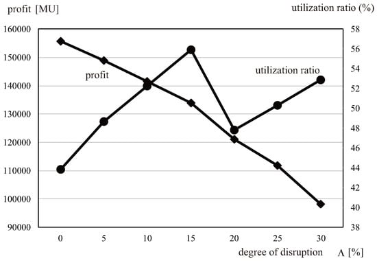
Figure 3. Profit and utilization ratio of facilities. Profit is expressed in monetary units [MU] and utilization ratio is expressed in percentages [%].

Table 1 and Figure 3 show that the profit decreases as the degree of disruption increases. In other words, a trade-off exists between profit maximization and adaptability to supply chain disruptions. When the degree of disruption is $\mathrm{\Lambda }=20$, the utilization ratio of the facilities decreases because the facilities are added. By contrast, the utilization ratio of the facilities increases as the degree of disruption increases. This indicates that more facilities are opened to deal with the supply chain disruptions. Although the number of opening facilities is generally restrained because lower costs are preferable for profit maximization, more facilities must be opened to deal with the supply chain disruptions and perform proper product delivery to customers. Even if the degree of disruption and the number of unavailable facilities increase, the number of facilities to be opened must be increased to maintain the supply levels to customers.

For example, if the degree of disruption is $\mathrm{\Lambda }=10$, profit is maximized on the assumption that 10% of all the available facilities are unusable for some reason. While the profit is 155,636 when the degree of disruption is $\mathrm{\Lambda }=0$, when $\mathrm{\Lambda }=10$, we can obtain a supply chain configuration and distribution plan assuming that 10% of the available facilities are unusable. In this case, the profit becomes 141,611, decreasing by approximately 10%. The supply chain manager should then consider the following: whether it is only necessary for the manager to prepare a plan assuming 10% of the facilities are unusable, or whether the manager should examine a plan that can handle even if 15% of the facilities are unusable. In this computational experiment, the manager makes plans from the degrees of disruption $\mathrm{\Lambda }=5$ to $\mathrm{\Lambda }=30$ to determine how much profit reduction is to be sacrificed in response to the supply chain disruptions. Finally, the manager must decide what level of disruption to expect.

Table 1 shows that sales tend to slightly increase until the degrees of disruption $\mathrm{\Lambda }=15$, but decrease after $\mathrm{\Lambda }=20$. This phenomenon is presumed to occur due to the following reason: while profit is maximized by supplying more products, including external supply when the degree of disruption is relatively small, it is thought that if the degree of disruption is larger than $\mathrm{\Lambda }=15$, the sales decreases because the transportation ability decreases as the disruption increases. As for the transportation cost, the transportation cost increases as the degree of disruption increases. The opening cost of facilities and the inventory cost also increase as the degree of disruption increases. In contrast, under the service-preservation constraint (Equation (9)), external contracting tends to saturate early to secure the baseline service level; subsequent robustness at higher $\mathrm{\Lambda }$ is achieved mainly via rerouting, inventory buffers, and selective openings, so the contract cost varies only mildly compared with transportation, opening, and inventory costs. From these facts, as the number of unusable facilities increases, the supply chain disruptions can be managed by selecting more costly routes compared to transportation by the optimal route in case no disruptions exist and by holding more inventory.

Table 1 shows that sales tend to slightly increase until the degree of disruption reaches $\mathrm{\Lambda }=15$, but decrease thereafter. This non-monotonic behavior can be explained by threshold effects embedded in the optimization structure. For low to moderate disruption levels ($\mathrm{\Lambda }\le 15$), the model reallocates flows to alternative transportation routes and external suppliers, which can temporarily sustain or even increase sales despite higher costs. Beyond this threshold, three interacting mechanisms dominate: (i) transportation capacity constraints become binding, limiting feasible reallocations; (ii) the penalty terms for under- and oversupply magnify marginal losses as deviations accumulate; and (iii) reliance on newly added facilities—which incur higher opening costs by design in our procedure—reduces net profitability. Together, these effects generate an inflection around $\mathrm{\Lambda }=15$, after which both sales and profits decline, even if service levels are maintained via more expensive configurations.

For the sensitivity analysis, we provide additional probability distributions of supply and demand, such that the average is the same as in the abovementioned standard case. The variance is, however, doubled. In the standard case, the supply chain configuration and distribution planning problem (6) with constraint (9) becomes infeasible at $\mathrm{\Lambda }=25$. Furthermore, one factory, one warehouse, and one distribution center are added. In both cases of larger supply and demand variances, problem (6) with constraint (9) also becomes infeasible at $\mathrm{\Lambda }=25$. One factory, one warehouse, and one distribution center are also added. At $\mathrm{\Lambda }=30$, problem (6) with constraint (9) also becomes infeasible. Therefore, more facility capacities are required compared to the standard case.

Table 2 shows each term of the objective function and the utilization rate of the facilities for case of larger supply and demand variances. With nonbinding external capacities, contracting saturates early under Equation (9), so contract cost remains comparatively flat across $\mathrm{\Lambda }$ (see the note before Table 1).

Table 2. Cases of larger supply and demand variances. Monetary values are expressed in monetary units [MU], transportation amounts in product units [PU], and percentages in [%].

Degree of Disruption	Profit	Sales	Cost				Number of Facilities Opened	Utilization Rate of Facilities
			Transportation	Opening	Contract	Inventory
Case of Larger Demand Variance
0	147,993	582,875	235,538	103,000	12,150	844	46.0	43.8
5	140,287	601,387	246,695	109,018	12,315	1294	48.7	48.7
10	133,821	607,315	254,167	109,018	12,849	1435	49.6	52.2
15	124,341	605,721	262,202	109,080	12,949	1578	50.0	45.0
20	114,421	602,956	269,018	109,630	12,962	1816	50.1	47.7
25	98,773	597,433	277,123	110,138	12,911	2190	50.2	50.2
30	87,487	595,476	284,053	112,482	12,800	2135	50.3	52.9
Cases of Larger Supply Variance
0	144,699	662,675	262,368	119,300	22,050	1548	54.0	51.4
5	136,663	671,054	271,972	122,398	22,931	1699	54.9	54.9
10	126,717	678,068	281,945	122,398	23,247	1969	56.0	59.0
15	114,870	674,374	289,729	123,498	23,008	2267	56.4	50.8
20	102,731	674,084	298,005	125,202	23,306	2556	56.9	54.2
25	91,958	674,010	303,281	130,308	23,402	2572	57.0	47.1
30	83,460	672,921	310,382	132,680	23,446	2254	55.8	48.1

Comparing Table 1 and Table 2, in the case of larger supply and demand variances, profit becomes smaller because larger uncertainties are dealt with. This impact is particularly greater in the case of the larger supply variance. The sales and costs considerably increase in the case of the larger supply variance compared to those in the case of demand variance. This is assumed to be due to the fact that the number of contracts with external suppliers increases to cope with the larger stochastic fluctuations in the supply. The number of opening facilities also increases in the case of the larger supply variance. More facilities must be opened for the larger stochastic fluctuations in the supply; hence, the supply chain manager must make plans that pay more attention to supply fluctuations.

3.2. Fractile Model

Similar to the expectation model, we perform 50 trials for each degree of disruption $\mathrm{\Lambda }$ in the fractile model. We change the assured probability level, which is a parameter for controlling the risk attitude of the supply chain manager, to $\theta =0.2,0.4,0.6$, and $0.8$.

Although a sensitivity analysis for more extreme values of $\theta$ (e.g., $\theta =0.1$ and $\theta =0.9$) was suggested, the computational burden for these extreme cases is significantly high due to the large-scale stochastic programming nature of the model, particularly when multiple disruption levels are considered. Therefore, instead of performing full numerical experiments, we provide a qualitative discussion of the expected tendencies: smaller $\theta$ values are likely to lead to configurations that maximize expected profit at the expense of increased variability, whereas larger $\theta$ values are expected to yield more conservative configurations with reduced variability in outcomes.

As a computational result of the fractile model without any disruption in the supply chain, Table 3 shows the profit, objective function value f, number of opening facilities, and number of contracts with external suppliers in each demand scenario. The numbers of opening facilities and contracts with external suppliers are represented by fractions. The denominator is the number of facilities that can be opened and the number of external suppliers that can be contracted. The numerator is the number of facilities that have been opened and the number of contracted external suppliers.

Table 3. Fractile model without any disruption. Monetary values are expressed in monetary units [MU], transportation amounts in product units [PU], and percentages in [%]. Values in “Number of Opening Facilities” and “Number of Contracts with External Suppliers” are written as numerator/denominator, where the numerator denotes the number actually opened (or contracted) and the denominator denotes the total number available.

$\theta$	0.2	0.4	0.6	0.8
f	163,785	161,170	158,738	156,154
$R^1$	128,185	134,470	140,938	147,254
$R^2$	137,085	143,370	149,838	156,154
$R^3$	145,985	152,270	158,738	156,354
$R^4$	154,885	161,170	159,138	156,254
$R^5$	163,785	161,170	158,738	156,154
expectation	145,985	150,490	153,478	154,434
Number of Opening Facilities
F	20/35	18/35	18/35	18/35
W	17/35	15/35	15/35	14/35
$D_C$	17/35	15/35	15/35	14/35
sum	54/105	48/105	48/105	46/105
Number of Contracts with External Suppliers
z	16/35	12/35	12/35	11/35

In Table 3, the assured probability level $\theta$ is smaller, which means the risk attitude of the supply chain manager becomes more risk-prone; therefore, the objective function value f is larger, and profit fluctuation for each scenario also becomes large. For example, when $\theta =0.2$, the objective function value is $f=163,785$, which is the largest compared to the other $\theta$ values. The profit at scenario $s^d=1$ is $R^1=128,185$, which is the minimum among all scenarios and is 78% of $f=163,785$. In contrast, when $\theta =0.8$, the objective function value is $f=156,154$, which is the smallest compared to the other $\theta$ values. The profit at scenario $s^d=1$ is $R^1=147,254$, which is the minimum and is 94% of $f=156,154$. If the manager who is risk-prone specifies a small assured probability level, say $\theta =0.2$, although the profit may be large at a certain scenario, it might be quite small at the other scenarios. Conversely, if the manager who is risk-averse specifies a large assured probability level, say $\theta =0.8$, the risk of an extremely small profit is reduced. The results in Table 3 imply that the fractile model represented by problem (8) works appropriately.

The non-monotonic tendencies observed in the expectation model also appear under the fractile model. At moderate disruption levels, the feasible reallocation of flows—now conditioned by the assured probability level $\theta$—can sustain sales, whereas at higher $\mathrm{\Lambda }$ values the compounded effects of binding capacity constraints, amplified penalty costs, and elevated opening costs of added facilities dominate. This indicates that the observed patterns are structural properties of the formulations rather than artifacts of particular simulation draws.

The numbers of opening facilities and contracts with external suppliers increase as the $\theta$ value decreases. A small $\theta$ value shows that the manager is risk-prone. Accordingly, the profit at a scenario with a larger demand is maximized. To deal with this situation, the numbers of opening facilities and contracts with external suppliers are increased.

As in the expectation model, we change the degree of disruption $\mathrm{\Lambda }$ from 0% to 30% by 5%, perform 50 trials for each degree of disruption $\mathrm{\Lambda }$, and discuss the computational results. When $\theta =0.2$, problem (8) becomes infeasible in the case of the degree of disruption $\mathrm{\Lambda }=20$. It becomes infeasible in the case of $\mathrm{\Lambda }=25$ again, and then we solve problem (8) with additional facilities. When $\theta =0.4,0.6$, and $0.8$, problem (8) becomes infeasible in cases $\mathrm{\Lambda }=20$ and 30. Problem (8) with additional facilities is solved in a similar manner.

Figure 4 shows the boxplots of 250 data points on the profits for the five scenarios in the 50 trials in the case of the minimum degree of disruption $\mathrm{\Lambda }=5$ and the maximum degree of disruption $\mathrm{\Lambda }=30$. The upper end of a boxplot represents the maximum value. The lower end represents the minimum value. Four intervals can be found between the minimum and maximum values, and each contains 25% of the total data. The horizontal axis depicts the assured probability level (i.e., $\theta =0.2,0.4,0.6$, and $0.8$). For comparison, the far right shows the result of the expectation model. Figure 5 illustrates the maximum, average, and minimum profits for all degrees of disruption $\mathrm{\Lambda }$ when $\theta =0.2$ and $\theta =0.8$.

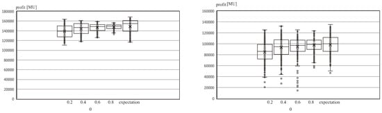
Figure 4. Profit distribution: $\mathrm{\Lambda }=5$ (left) and $\mathrm{\Lambda }=30$ (right). Profit is expressed in monetary units [MU].

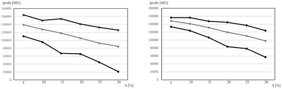
Figure 5. Distribution of profit: $\theta =0.2$ (left) and $\theta =0.8$ (right). Profit is expressed in monetary units [MU].

In Figure 4 and Figure 5, the profit decreases as the degree $\mathrm{\Lambda }$ increases. Its variance also becomes large. The profit variance is suppressed as the assured probability level $\theta$ increases (i.e., the manager is more risk-averse). If the manager with a risk-averse preference specifies a large assured probability level (e.g., $\theta =0.8$), the variance of the bottom 25% of profit is considerably suppressed. Moreover, the profit minimum becomes large compared to the other assured probability levels.

The abovementioned result depicts that the supply chain manager, who does not want to take the risk of extremely small profits, can make decisions that match his or her own preference by specifying a relatively large assured probability level (e.g., $\theta =0.8$). Conversely, if the risk-prone manager specifies a small assured probability level (e.g., $\theta =0.2$), a high profit can be obtained despite the increasing profit variance. However, as can be seen from the right side of Figure 4 for the case of $\mathrm{\Lambda }=30$, compared to the result of the expected value model, the values of the top 25% of profits do not increase, and the profit minimum is smaller. Therefore, the risk-prone manager should pay attention to the risk of low profits when the supply chain disruptions become too large. In particular, with relatively large disruptions in the supply chain (e.g., degree of disruption $\mathrm{\Lambda }=20$ and so on), the profit maximum for $\theta =0.2$ and that for $\theta =0.8$ are almost at the same level. The profit minimum for $\theta =0.8$ is rather larger than that for $\theta =0.2$. The advantage for the manager to specify a small value of the assured probability level (e.g., $\theta =0.2$) is quite small when the manager should prepare for relatively large disruptions.

Regarding the utilization ratio of the facilities, problem (8) is infeasible in the case of $\mathrm{\Lambda }=20$. We add facilities and show the results of the case of $\mathrm{\Lambda }=5$ and $\mathrm{\Lambda }=15$ in Figure 6, where the number of data for boxplots is 50 data points of 50 trials because the decisions on opening facilities are variables at the first stage.

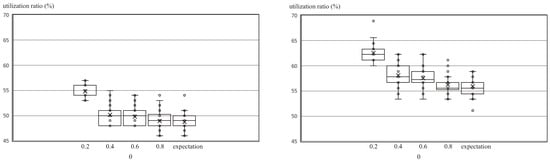
Figure 6. Distributions of Utilization Ratio of Facilities: $\mathrm{\Lambda }=5$ (left) and $\mathrm{\Lambda }=15$ (right). Utilization ratio is expressed in percentages [%].

Figure 6 shows that, compared to that in the case of $\mathrm{\Lambda }=5$, the utilization ratio of the facilities in the case of $\mathrm{\Lambda }=15$ increases along with its variance. As the assured probability level $\theta$ increases with a stronger risk-averse preference, the utilization ratio of the facilities decreases. As shown by the computational result of the profit, for the utilization ratio of the facilities, the manager can make decisions according to his/her own preference by appropriately specifying the assured probability level.

Figure 7 illustrates the maximum, average, and minimum numbers of opening facilities for $\theta =0.2$ and $\theta =0.8$. For reference, the number of opening facilities without disruptions is indicated by a dashed line.

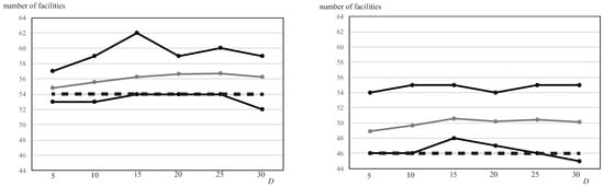
Figure 7. Distributions of utilization ratio of facilities: $\theta =0.2$ (left) and $\theta =0.8$ (right). Utilization ratio is expressed in percentages [%].

The dashed lines for both $\theta =0.2$ and $\theta =0.8$ are around the minimum number; hence, more facilities are needed if supply chain disruptions occur. When $\theta =0.2$, in which the manager is risk-prone, and as analyzed for the optimal solution in the case without disruption, it is necessary to open more facilities to pursue profit maximization compared to $\theta =0.8$.

3.3. Theoretical and Practical Implications

This subsection explains how our results answer the research question and what they imply for theory and practice. Recall that the disruption degree $\mathrm{\Lambda }$ denotes the share of facilities that become unavailable (we vary $\mathrm{\Lambda }\in \{0,5,\dots ,30\}\%$), and the assured probability level $\theta \in (0,1]$ controls risk in the fractile model. Equation (9) is the service-preservation constraint that enforces, for each product–customer–period, the shipped amount under disruptions to be no smaller than the baseline (no-disruption) plan.

• Theoretical implications

(i)

Enforcing Equation (9) under exogenous $\mathrm{\Lambda }$ yields a transparent profit–adaptability frontier that is distinct from classic expected-value bi-objective (cost vs. revenue) formulations. Empirically, profit decreases monotonically as $\mathrm{\Lambda }$ increases, while the utilization of opened facilities rises (Table 1; Figure 3), making the preparedness–profit trade-off explicit rather than implicit in the objective.

(ii)

The fractile (quantile) formulation (Equations (8) and (11)) provides a tunable risk device. Increasing $\theta$ tightens the lower tail of the profit distribution (i.e., raises the minimum and reduces dispersion), whereas smaller $\theta$ may improve the upper tail at the expense of higher variability (Figure 4 and Figure 5). Thus, managerial risk attitude is mapped directly to outcome distributions through $\theta$.

(iii)

Combining two-stage recourse (first-stage openings/contracts; second-stage routing/inventory) with disruption simulation (Section 2.2.3) offers a tractable way to approximate biased, region/time-clustered outages (Section 2.2.4) without exploding joint scenario counts, preserving solvability on multiperiod, multi-echelon instances.

(iv)

Sensitivity analysis shows that supply-side variance is more damaging than demand-side variance of similar magnitude (Table 2), theoretically motivating asymmetric hedging on the supply side (e.g., standby capacity or contracts).

• Practical implications

(i)

Managers can co-tune $(\mathrm{\Lambda },\theta )$ to align preparedness and risk attitude: pick $\mathrm{\Lambda }$ as the target disruption level (e.g., 15–$20\%$) and set $\theta$ to cap downside profit. In our baseline expectation model, feasibility pressure emerges around $\mathrm{\Lambda }\approx 20\%$ (Table 1), indicating where contingency capacity is likely required.

(ii)

Service preservation as $\mathrm{\Lambda }$ grows is primarily achieved by (a) opening more facilities, (b) using costlier routes, and (c) holding additional inventory (Table 1). On average, the number of external contracts increases only mildly, suggesting that capacity and routing buffers are the first-order levers.

(iii)

When supply variance doubles, both external contracts and openings rise more sharply than under increased demand variance (Table 2). A practical rule-of-thumb is to prioritize upstream (supply-side) hedges—e.g., standby contracts and additional DC capacity—over purely demand-side buffers when upstream uncertainty dominates.

(iv)

If infeasibility appears at higher $\mathrm{\Lambda }$ levels, adding one facility per layer at a surcharge restored feasibility in our setting (Section 3.1), providing a budgetary stress-test guideline for minimal augmentation.

4. Conclusions

This study develops TSA-SCD (Two-Stage Analysis for Supply Chain Disruptions), a two-stage stochastic optimization framework for supply chain network design under disruption risks. The framework comprises an expectation model (Equation (6)) and a fractile (quantile) model (Equations (8) and (11)), and enforces a service-preservation constraint (Equation (9)) at an exogenously chosen disruption degree $\mathrm{\Lambda }$. Decision-making explicitly considers the trade-off between profit maximization and the ability to adapt to supply chain disruptions, while the assured probability level $\theta$ in the fractile model maps managerial risk attitude to the lower tail of profit.

We model the problem as a two-stage stochastic program with simple recourse. In the first stage, facility openings and contracts with external suppliers are selected. In the second stage, after demand (and optionally supply; see Section 2.2.4) scenarios are realized and disruptions are simulated according to $\mathrm{\Lambda }$, distribution and inventory decisions are optimized subject to Equation (9).

We conduct computational experiments varying the disruption degree $\mathrm{\Lambda }\in \{0,5,\dots ,30\}\%$ and the assured probability level $\theta \in \{0.2,0.4,0.6,0.8\}$. The results reveal: (i) higher $\mathrm{\Lambda }$ reduces profit monotonically and increases utilization, highlighting the economic cost of preparedness; (ii) larger $\theta$ (more risk-averse) tightens the lower tail of profit and suppresses dispersion; (iii) smaller $\theta$ (more risk-prone) can raise the upper tail but increases the chance of poor outcomes under severe disruptions; and (iv) feasibility pressure emerges near $\mathrm{\Lambda }\approx 20\%$, where minimal capacity augmentation restores feasibility.

The contributions are threefold: (1) an integrated framework that unifies expected-value and quantile-based decision-making, allowing managers to co-tune $(\mathrm{\Lambda },\theta )$; (2) a practical instantiation of the fractile model that tunes downside profit through $\theta$ and reveals a profit–adaptability frontier induced by Equation (9); and (3) quantitative insights into how disruption degree and risk preference shape openings, external contracts, routing, inventory, and profit distributions in multiperiod, five-echelon networks with external suppliers.

Future research should address several limitations and extensions of the present study. First, the model assumes binary treatment of facility opening and contracting decisions. While this assumption facilitated tractable optimization and clear interpretation of disruption scenarios, it does not capture partial capacity restoration or phased reopening. Introducing multilevel or continuous decision variables could better represent practical recovery processes in disrupted supply chains. In addition, promising directions include modeling correlated and cascading disruptions, incorporating dynamic recovery and relocation processes, conducting empirical validations, exploring alternative risk measures such as CVaR, and integrating more deeply with inventory policies, demand management, and mode selection. Beyond the tactical scope adopted here, a natural extension is a genuinely multistage design with period-by-period reopening/closure and dynamic recovery; promising directions include SDDP-/PHA-based implementations of these variants and the integration of CVaR (and other coherent risk measures) into TSA-SCD to explicitly manage tail-average losses under severe disruptions.

References

- Wierzbicki, A.P. The use of reference objectives in multiobjective optimization. In Multiple Criteria Decision Making: Theory and Application; Fandel, G., Gal, T., Eds.; Springer: Berlin/Heidelberg, Germany, 1980; pp. 468–486. [Google Scholar]
- Ignizio, J.P. Linear Programming in Single- & Multiple Systems; Prentice-Hall: Englewood Cliffs, NJ, USA, 1982. [Google Scholar]
- Zeleny, M. Multiple Criteria Decision Making; McGraw-Hill: New York, NY, USA, 1982. [Google Scholar]
- Chankong, V.; Haimes, Y.Y. Multiobjective Decision Making: Theory and Methodology; Dover Publications: Mineola, NY, USA, 1983. [Google Scholar]
- Sawaragi, Y.; Nakayama, H.; Tanino, T. Theory of Multiobjective Optimizations; Academic Press: New York, NY, USA, 1985. [Google Scholar]
- Yu, P.L. Multiple-Criteria Decision Making: Concepts, Techniques, and Extensions; Plenum Press: New York, NY, USA, 1985. [Google Scholar]
- Steuer, R.E. Multiple Criterion Optimization: Theory, Computation, and Application; John Wiley & Sons: New York, NY, USA, 1986. [Google Scholar]
- Seo, F.; Sakawa, M. Multiple Criteria Decision Analysis in Regional Planning: Concepts, Methods and Applications; D. Reidel Publishing Company: Dordrecht, The Netherlands, 1988. [Google Scholar]
- Stadler, W. (Ed.) Multicriteria Optimization in Engineering and in the Sciences; Plenum Press: New York, NY, USA, 1988. [Google Scholar]
- Haimes, Y.Y.; Tarvainen, K.; Shima, T.; Thadathil, J. Hierarchical Multiobjective Analysis of Large-Scale Systems; Hemisphere: New York, NY, USA, 1990. [Google Scholar]
- Sakawa, M. Fuzzy Sets and Interactive Multiobjective Optimization; Plenum Press: New York, NY, USA, 1993. [Google Scholar]
- Weber, C.A.; Current, J.R. A multi-objective approach to vendor selection. Eur. J. Oper. Res. 1993, 68, 173–184. [Google Scholar] [CrossRef]
- Jayaraman, V. A multi-objective logistics model for a capacitated service facility problem. Int. J. Phys. Distrib. Logist. Manag. 1999, 29, 65–81. [Google Scholar] [CrossRef]
- Korpela, J.; Kylaheiko, K.; Lehmusvaara, A.; Touminen, M. An analytic approach to production capacity allocation and supply chain design. Int. J. Prod. Econ. 2002, 78, 187–195. [Google Scholar] [CrossRef]
- Erol, I.; Ferrell, W.G., Jr. A methodology to support decision making across the supply chain of an industrial distributor. Int. J. Prod. Econ. 2004, 89, 119–129. [Google Scholar] [CrossRef]
- Erol, I.; Ferrell, W.G., Jr. A methodology for selection problems with multiple, conflicting objectives and both qualitative and quantitative criteria. Int. J. Prod. Econ. 2003, 86, 187–199. [Google Scholar] [CrossRef]
- Zhou, G.; Min, H.; Gen, M. A genetic algorithm approach to the bi-criteria allocation of customers to warehouses. Int. J. Prod. Econ. 2003, 86, 35–45. [Google Scholar] [CrossRef]
- Azaron, A.; Brown, K.N.; Tarim, S.A.; Modarres, M. A multi-objective stochastic programming approach for supply chain design considering risk. Int. J. Prod. Econ. 2008, 116, 129–138. [Google Scholar] [CrossRef]
- Liao, Z.; Rittscher, J. A multi-objective supplier selection model under stochastic demand conditions. Int. J. Prod. Econ. 2007, 105, 150–159. [Google Scholar] [CrossRef]
- Demirtas, E.A.; Ustun, O. An integrated multiobjective decision making process for supplier selection and order allocation. Omega 2008, 111, 378–388. [Google Scholar] [CrossRef]
- Franca, R.B.; Jones, E.C.; Richards, C.N.; Carlson, J.P. Multi-objective stochastic supply chain modeling to evaluate tradeoffs between profit and quality. Int. J. Prod. Econ. 2010, 127, 292–299. [Google Scholar] [CrossRef]
- Pishvaee, M.S.; Torabi, S.A. A possibilistic programming approach for closed-loop supply chain network design under uncertainty. Fuzzy Sets Syst. 2010, 161, 2668–2683. [Google Scholar] [CrossRef]
- Liu, S.; Papageorgiou, L.G. Multiobjective optimisation of production, distribution and capacity planning of global supply chains in the process industry. Omega 2013, 41, 369–382. [Google Scholar] [CrossRef]
- Huang, E.; Goetschalckx, M. Strategic robust supply chain design based on the Pareto-optimal tradeoff between efficiency and risk. Eur. J. Oper. Res. 2014, 237, 508–518. [Google Scholar] [CrossRef]
- Zhuang, X.; Wang, Y.; Li, J. Two-stage stochastic programming with robust constraints for post-disruption logistics network design. Asia-Pac. J. Oper. Res. 2023, 40, 2350032. [Google Scholar]
- Yang, G.-Q.; Liu, Y.-K.; Yang, K. Multi-objective biogeography-based optimization for supply chain network design under uncertainty. Comput. Ind. Eng. 2015, 85, 145–156. [Google Scholar] [CrossRef]
- Pasandideh, S.H.R.; Niaki, S.T.A.; Asadi, K. Bi-objective optimization of a multi-product multi-period three-echelon supply chain problem under uncertain environments: NSGA-II and NRGA. Inf. Sci. 2015, 292, 57–74. [Google Scholar] [CrossRef]
- Moayedi, M.; Rasti-Barzoki, M.; Sadeghi, H. Multi-objective stochastic programming for sustainable supply chain design under demand and supply uncertainty. J. Clean. Prod. 2023, 382, 135375. [Google Scholar]
- Nooraie, S.V.; Parast, M.M. Mitigating supply chain disruptions through the assessment of trade-offs among risks, costs and investments in capabilities. Int. J. Prod. Econ. 2016, 171, 8–21. [Google Scholar] [CrossRef]
- Hu, H.; Feng, Y.; Chen, X.; Wang, Z. Two-stage stochastic programming model for resilient supply chain network design under facility disruptions. Comput. Ind. Eng. 2023, 177, 108044. [Google Scholar]
- Kungwalsong, K. Two-stage stochastic program for multi-layer supply chain network design under facility disruptions. Sustainability 2021, 13, 12654. [Google Scholar] [CrossRef]
- Tolooie, A.; Maity, M.; Sinha, A.K. A two-stage stochastic mixed-integer program for reliable supply chain network design under uncertain disruptions and demand. Comput. Ind. Eng. 2020, 148, 106722. [Google Scholar] [CrossRef]
- Santibañez-Aguilar, J.E.; Morales-Rodriguez, R.; González-Campos, J.B.; Ponce-Ortega, J.M. Stochastic design of biorefinery supply chains considering economic and environmental objectives. J. Clean. Prod. 2016, 136, 224–245. [Google Scholar] [CrossRef]
- Taghvaei, D.; Rezapour, S.; Samani, M. Bi-objective two-stage stochastic programming for resilient humanitarian relief supply chains under uncertainty. Comput. Ind. Eng. 2025, 192, 109089. [Google Scholar]
- Hombach, L.E.; Büsing, C.; Walther, G. Robust and sustainable supply chains under market uncertainties and ds—A case study of the German biodiesel market. Eur. J. Oper. Res. 2018, 269, 302–312. [Google Scholar] [CrossRef]
- Sawik, T. Stochastic optimization of supply chain resilience with disruption risk. Omega 2022, 110, 102614. [Google Scholar]
- OECD. Supply Chain Resilience Review; Organisation for Economic Co-operation and Development: Paris, France, 2025. [Google Scholar]
- Nicoletti, J.; You, F. Multiobjective economic and environmental optimization of global crude oil purchase and sale planning with noncooperative stakeholders. Appl. Energy 2020, 259, 114222. [Google Scholar] [CrossRef]
- Karimi, H.; Ekşioğlu, S.D.; Carbajales-Dale, M. A biobjective chance constrained optimization model to evaluate the economic and environmental impacts of biopower supply chains. Ann. Oper. Res. 2021, 296, 95–130. [Google Scholar] [CrossRef]
- Meng, L.; Yang, H.; Zhang, C. Two-stage chance constrained stochastic programming for humanitarian relief logistics under uncertainty. Transp. Res. Part E Logist. Transp. Rev. 2023, 167, 102957. [Google Scholar]
- Guo, Y.; Wang, H.; Chen, F. Supply chain resilience: A review from inventory management perspective. Sustain. Oper. Comput. 2025, 6, 200046. [Google Scholar] [CrossRef]
- McDougall, N.; Bell, S.; Howard, L. The local supply chain during disruption: Lessons from recent crises. J. Clean. Prod. 2024, 430, 139515. [Google Scholar]
- Alvarez, A.; Cordeau, J.-F.; Jans, R.; Munari, P.; Morabito, R. Inventory routing under stochastic supply and demand. Omega 2021, 102, 102304. [Google Scholar] [CrossRef]
- Geoffrion, A.M. Stochastic programming with aspiration or fractile criteria. Manag. Sci. 1967, 31, 672–679. [Google Scholar] [CrossRef]
- Kataoka, S. A stochastic programming model. Econometrica 1967, 31, 181–196. [Google Scholar] [CrossRef]
- Das, D.; Bandyopadhyay, S.; Bhattacharya, A. Risk-averse two-stage stochastic programming using CVaR for closed-loop supply chain network design. Comput. Ind. Eng. 2022, 165, 107929. [Google Scholar]
- Pavlikov, K.; Veremyev, A.; Pasiliao, E.L. Optimization of Value-at-Risk: Computational aspects of MIP formulations. J. Oper. Res. Soc. 2018, 69, 676–690. [Google Scholar] [CrossRef]
- Moorad, C. An Introduction to Value-at-Risk, 5th ed.; Wiley: Hoboken, NJ, USA, 2013. [Google Scholar]
- Pflug, G.C. Some remarks on the value-at-risk and the conditional value-at-risk. In Probabilistic Constrained Optimization; Kluwer: Alphen aan den Rijn, The Netherlands, 2000; pp. 271–281. [Google Scholar]
- Rahimi, M.; Baboli, S.; Dolgui, A. Risk-averse sustainable supply chain network design with CVaR and reliability considerations. Comput. Ind. Eng. 2019, 129, 512–526. [Google Scholar]
- Romanko, O.; Mausser, H. Robust scenario-based value-at-risk optimization. Ann. Oper. Res. 2016, 237, 203–218. [Google Scholar] [CrossRef]
- Zou, J.; Ahmed, S.; Sun, X.A. Stochastic dual dynamic programming. Math. Program. Ser. A 2019, 175, 461–502. [Google Scholar] [CrossRef]
- Rockafellar, R.T. Progressive Hedging in Stochastic Optimization; Tutorial Notes; Department of Mathematics, University of Washington: Seattle, WA, USA, 2017. [Google Scholar]
Disclaimer/Publisher’s Note: The statements, opinions and data contained in all publications are solely those of the individual author(s) and contributor(s) and not of MDPI and/or the editor(s). MDPI and/or the editor(s) disclaim responsibility for any injury to people or property resulting from any ideas, methods, instructions or products referred to in the content. |
© 2025 by the authors. Licensee MDPI, Basel, Switzerland. This article is an open access article distributed under the terms and conditions of the Creative Commons Attribution (CC BY) license (https://creativecommons.org/licenses/by/4.0/).