A Simulated Weather-Driven Bio-Economic Optimization Model for Agricultural Planning

Abstract

This study develops a weather-driven bio-economic optimization framework for agricultural planning in Guyana by integrating weather simulation, crop modeling, and multi-objective optimization. Precipitation was modeled using a first-order Markov chain with fitted distribution, while temperature and relative humidity were simulated using stochastic differential equations. Reference evapotranspiration was estimated using an artificial neural network. These simulated weather variables were then used as inputs to AquaCrop to estimate rice, maize, and soybean yields across multiple planting intervals. A multi-objective optimization model was then applied to optimize gross profit, economic water productivity, and land use efficiency. Validation at the Rose Hall Estate showed strong accuracy for rice and maize (MAPE < 10%) and moderate accuracy for soybeans. Scenario analyses for the 2024–2025 season, assuming 25% and 50% export targets, revealed that rice–maize double cropping produced the highest profitability, while soybean–maize combinations were less favorable. The framework replaces static yield assumptions with dynamic, simulation-driven models that incorporate price forecasts and allow substitution of alternative forecasting or crop simulators to enhance precision. The scenario-based design provides a flexible decision-support platform for optimizing crop selection, planting intervals, and resource allocation under climate variability and market uncertainty. Moreover, the framework is scalable and well-suited for evidence-based agricultural planning.

1. Introduction

Agricultural crop production is a cornerstone of food security, sustainable development, and economic stability. In tropical countries, where climatic conditions support year-round cultivation, farming serves as the primary livelihood for much of the population and remains a key driver of rural economies. In the tropical nation of Guyana, agriculture plays a vital role in the national economy, employing approximately 17% of the labor force and accounting for nearly 25% of non-oil GDP [1]. Historically, traditional farming practices dominated crop production across the country. However, over the past two decades, there has been a significant transition toward more modern and technology-driven approaches. This transition reflects the growing need to enhance productivity, improve resource efficiency, and ensure sustainability. Key transformations include the adoption of mechanization, expanded large-scale crop production for export, and the implementation of precision agriculture techniques to improve efficiency and resource management.

Precision agriculture, which emphasizes the use of technology and data analytics and simulation tools, is therefore essential for optimizing crop production and ensuring long-term agricultural resilience. A core component of precision agriculture is agricultural planning, which addresses strategic questions regarding what crops to plant, when to plant them, where to allocate land, and how much to produce. In Guyana, as in many other tropical countries, these decisions present significant challenges for both farmers and policymakers, who must balance economic objectives with effective use of land, water, and other critical resources.

Optimizing profit and economic productivity from water resources, while efficiently using available land, are central objectives for agricultural decision-makers. In practice, however, these objectives often conflict, resulting in trade-offs between profitability and resource sustainability. Addressing agricultural planning under such competing objectives naturally leads to a multi-objective optimization problem, which provides a structured and quantitative framework for exploring these trade-offs.

When attempting to optimize profit, economic water productivity, and land use, several interrelated factors must be considered. These include crop yield, unit price of output, production costs, and the crop’s evapotranspiration rate during growth. Among these, accurately determining crop yield is often the most complex and influential task, as it depends on a wide range of supplemental variables such as soil type, field management practices, crop characteristics, cultivar selection, irrigation method, planting date, and, most critically, weather conditions. Because weather is highly variable and beyond human control, it introduces substantial uncertainty that must be explicitly accounted for in any agricultural planning framework.

These uncertainties, however, can be effectively addressed through statistical, mathematical, and machine learning approaches that simulate weather behavior and generate reliable projections of key climatic variables. By accurately capturing the temporal dynamics of weather conditions and integrating these results with other agronomic and management factors in a crop growth simulator, it becomes possible to estimate both current and future crop yields under varying environmental scenarios.

Crop growth simulators, which are used to simulate crop yield and biomass development, can estimate yields across different planting periods and climatic conditions while also computing the corresponding total evapotranspiration. By linking the projected yields generated by these simulators together with simulated weather data, market prices, and production costs, agricultural planners can better address fundamental questions regarding optimal crop selection and planting schedules. Through this integration, agricultural planning can transition from static, assumption-based frameworks to dynamic, scenario-driven systems that better capture environmental variability and risk.

Recent works in stochastic agricultural modeling have demonstrated the value of incorporating weather uncertainty, scenario ensembles, and optimization techniques into farm- and regional-level decision-making. For instance, stochastic programming has been used to optimize irrigation and agronomic decisions under uncertain precipitation, crop prices, and water availability [2]. Weather-driven scenario analysis has been applied to irrigation scheduling, combining multiple stochastic climate realizations with crop simulation models to improve risk-aware water management [3]. Bio-economic simulation under uncertainty has also been explored by integrating stochastic environmental states with crop–soil process models to evaluate irrigation profitability and farm-scale outcomes [4]. Similarly, stochastic statistical models have been applied to crop planning and agricultural resource management [5], while scenario-based stochastic optimization combined with crop simulation has been employed to assess planting strategies, nitrogen management, and cultivar choice [6].

Despite these contributions, no studies have yet integrated stochastic climate simulation, crop modeling, and multi-objective optimization into a single unified framework. This integrated approach, combining climate modeling, yield simulation, and optimization, holds significant promise as a decision-support tool to guide agricultural planning, resource allocation, and policy formulation in the face of climate variability and economic uncertainty.

Building upon these insights and addressing the identified research gap, this study develops a weather-driven bio-economic optimization model to support agricultural planning and decision-making in tropical contexts such as Guyana, where decisions are often made with limited integration of analytical, statistical, or model-based insights. The model integrates the following three major components: (i) stochastic weather modeling using Markov chains for precipitation and Ornstein–Uhlenbeck processes for temperature and humidity [7,8,9]; (ii) artificial neural network (ANN)-based estimation of reference evapotranspiration (ETo) [10,11,12,13,14,15,16,17,18]; and (iii) a multi-objective optimization (MOO) framework utilizing the NSGA-II algorithm to maximize profitability, optimize ET economic water productivity (EEWP), and minimize land use [19,20]. Unlike previous agricultural optimization models that rely on historical or static yield data and deterministic inputs [19,20,21], this framework dynamically integrates simulated weather, AquaCrop-based yield predictions, and time-series price forecasts to provide a more realistic and forward-looking planning tool.

Applied to Rose Hall Estate in East Berbice-Corentyne, Guyana, this research demonstrates how integrating weather simulations, crop growth modeling, and optimization enables actionable insights for both farmers and policymakers. By presenting a modular framework that can incorporate alternative forecasting techniques, weather models, crop simulators, and optimization algorithms, this study contributes a flexible decision-support platform designed to enhance agricultural resilience in the face of climate variability and market uncertainty.

The remainder of this paper is organized as follows: Section 2 outlines the study area, data, model design, and a description of AquaCrop; Section 3 presents the results of the weather models, crop simulations, and multi-objective optimization; Section 4 discusses the findings, limitations, and future work; and Section 5 concludes the study.

2. Materials and Methods

2.1. Study Area and Weather Data

The weather data used for this study’s simulations were obtained from the New Amsterdam weather station and Climate Engine’s reanalysis dataset. Crop yield simulations and multi-objective optimization testing were conducted for agricultural lands in Rose Hall Estate, located approximately 4 km from the New Amsterdam station. This coastal site, situated in Guyana’s East Canje Berbice-Corentyne region, experiences two distinct rainy seasons from May to July and December to January. Temperatures remain relatively stable year-round, with monthly maximums consistently averaging 30 °C or higher. Rose Hall Estate, a former sugar plantation, spans roughly 3808 ha and is predominantly characterized by Whittaker 37 clay soils.

Precipitation simulations were based on reanalysis dataset from 1981 to 2022 due to the unavailability of long-term station rainfall records. The CHIRPS dataset, selected for its high spatial resolution ($4.8\mathrm{km}, 1/20°$), was used to construct the precipitation model. Observed weather data from the New Amsterdam station (2001–2022) were used for temperature and humidity modeling, as well as for reference evapotranspiration (ETo) estimation. These dataset included daily maximum and minimum temperatures, average dew point, and 2 m wind speed measurements.

The data needed for estimating ETo were calculated using [22] (Appendix A). The daily extraterrestrial radiation used was obtained from the Sirad package in R [23]. This function requires the Julian day and Latitude in radians as input parameters. Our study used latitudes of 6.243 (radians). About 0.5 percent of the data in the New Amsterdam dataset was missing. This was addressed using a K-nearest neighbour algorithm with K set to 5.

2.2. Crops Used in Simulation

The GRDB 10, a local rice variety with a yield potential of 6.8–7 tons per hectare, will be used along with corn and soybeans for the simulation. As there is no available information on the varieties of corn and soybeans currently under mass cultivation in Guyana, information concerning these crops will be sourced from the literature. Specifically for simulation purposes, the open-field Pollinated Yellow corn variety and the MSOY 9144 variety will be used for Maize and Soybeans, respectively. The parameters employed for the AquaCrop simulations are detailed in Table A9 and Table A10.

2.3. Schematic Diagram of Model Structure

Figure 1 illustrates the schematic structure of the modeling framework. The first stage represents the four climatic variables modeled: minimum temperature, maximum temperature, precipitation, and relative humidity. These variables were selected based on AquaCrop’s input requirements, with relative humidity additionally modeled to enhance the accuracy of the artificial neural network (ANN) used for estimating reference evapotranspiration (ETo).

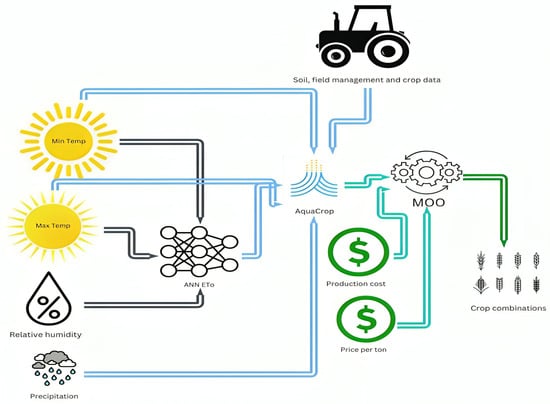
Figure 1. Schematic diagram of the weather-driven bio-economic optimization model.

The second stage of the framework depicts the ANN component for estimating ETo. After being trained and calibrated on observed data, the ANN was supplied with simulated data from the temperature and relative humidity models, together with solar radiation values estimated from the temperature data. This integration enabled the generation of simulated ETo values. The simulated ETo, along with simulated precipitation and temperature data, was then formatted into a text file and imported into AquaCrop to create a climate file. With this climate file in place, AquaCrop was configured with information on soil properties for the study area, crop parameters, and field management practices. Using these inputs, yields for each crop were simulated across multiple planting dates spaced approximately seven to eight days apart. The resulting outputs were then averaged to produce mean yield estimates for several planting intervals, each approximately 14–16 days in length.

Finally, the yield data for the various planting intervals, together with the corresponding ETo, production cost, and yield prices associated with each interval, were used to construct a dataset for the multi-objective optimization (MOO) model. In these dataset, each row represented a specific crop, its planting interval, and the associated cost and water use. The MOO model then simultaneously optimized three objectives: maximizing gross profit, maximizing ET-based economic water productivity, and minimizing total land use, subject to constraints on land availability, water resources, and market demand. The optimization process generated a set of Pareto-optimal cropping combinations that balanced profitability, water efficiency, and land utilization.

2.4. Precipitation Model

Daily precipitation was simulated using a stochastic two-step approach: (i) a first-order Markov chain to model rainfall occurrence, and (ii) probability distributions to estimate rainfall amounts on wet days. Four candidate distributions; the lognormal, Weibull, and two- and three-parameter gamma, were evaluated. To account for seasonal rainfall variability, the dataset was divided into 12 monthly subsets, with separate fits performed for each month. The best-fitting distribution was selected using the Akaike Information Criterion (AIC) [24] and probability–probability (PP) plots, ensuring an accurate representation of seasonal precipitation patterns.

2.4.1. Precipitation Occurrence Model

Rainfall occurrence was modeled as a binary sequence of wet (1) and dry (0) days, where transition probabilities between states were estimated using a first-order Markov chain. Higher-order chains can marginally improve performance, but their added computational complexity provides minimal benefit. Thus, a first-order model was selected [9]. The Markov property states that the probability of precipitation on day $t+1$ depends only on the state of day t:

$$P(X_{t+1}=s_{t+1}\mid X_t=s_t,X_{t-1}=s_{t-1},\dots )=P(X_{t+1}=s_{t+1}\mid X_t=s_t),$$

(1)

where $s\in \{d,w\}$ denotes dry (d) and wet (w) states, and $t\in \{0,1,2,\dots ,T\}$.

The transition probabilities are summarized in the matrix P:

$$\mathbf{P}=\left[\begin{array}{cc}{p}_{dd}& p_{dw}\\ p_{wd}& p_{ww}\end{array}\right],0\le p_{ij}\le 1,$$

(2)

with row sums constrained to one:

$$\sum _{j=1}^S{P}_{ij}=1,i\in \{d,w\}.$$

(3)

The elements are defined as:

$$P_{dd}=P(\mathrm{dry}\mathrm{on}\mathrm{day}t+1\mid \mathrm{dry}\mathrm{on}\mathrm{day}t),P_{dw}=P(\mathrm{wet}\mathrm{on}\mathrm{day}t+1\mid \mathrm{dry}\mathrm{on}\mathrm{day}t),$$

$$P_{wd}=P(\mathrm{dry}\mathrm{on}\mathrm{day}t+1\mid \mathrm{wet}\mathrm{on}\mathrm{day}t),P_{ww}=P(\mathrm{wet}\mathrm{on}\mathrm{day}t+1\mid \mathrm{wet}\mathrm{on}\mathrm{day}t).$$

Because only two states exist, probabilities are complementary; for example, $p_{ww}=1-p_{wd}$.

The stationary distribution $\pi =({\pi }_d,{\pi }_w)$ satisfies $\pi =\pi \mathbf{P}$, where ${\pi }_d$ and ${\pi }_w$ represent the long-term probabilities of dry and wet states, respectively:

$${\pi }_d={\displaystyle \frac{p_{wd}}{p_{wd}+p_{dw}}},{\pi }_w={\displaystyle \frac{p_{dw}}{p_{wd}+p_{dw}}}.$$

(4)

2.4.2. Rainfall Amount Modeling

Rainfall amounts on wet days were modeled by fitting candidate parametric distributions to the stratified monthly datasets. Although the gamma distribution is widely used for precipitation modeling [8,25,26,27,28], precipitation in tropical climates exhibits strong seasonal variability. Several hydrological studies have shown that no single probability distribution consistently fits rainfall across all months or regions. Consequently, the suitability of a distribution often depends on the rainfall regime and the statistical characteristics of wet-day amounts. This variability has been demonstrated in tropical rainfall analyses using satellite-derived rain rates [29], in monthly rainfall modeling across Bangladesh where the best-fit distribution varied with climatic conditions [30], and in studies from the Lake Toba region where Gamma, Lognormal, and Weibull distributions performed best in different months and locations [31].

Given the positive skewness observed in rainfall amounts—as seen in Figure 2, the Weibull, two-parameter gamma, three-parameter gamma, and lognormal distributions were selected as candidate distributions because of their theoretical suitability for positively skewed precipitation data and their widespread use in tropical rainfall modeling. Each of these four distributions was fitted to every month of the dataset, and the best-fitting distribution for each month was determined using the Akaike Information Criterion (AIC) and probability–probability (P–P) plots. Parameters for each distribution were estimated via maximum likelihood estimation (MLE) [8,9,25,26,28].

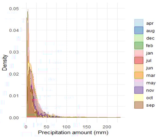
Figure 2. Density plot of precipitation over Rose Hall (1981–2022).

2.4.3. Probability Distributions

• Lognormal Distribution

The lognormal distribution is a positively skewed continuous probability distribution commonly used to model variables such as precipitation amounts, where values are strictly non-negative. If a random variable X is lognormally distributed, then $Y=ln\left(X\right)$ follows a normal distribution. The probability density function (PDF) is given by:

$$f_{LN}(x;\mu ,\sigma )={\displaystyle \frac{1}{x\sigma \sqrt{2\pi }}}exp\left(-{\displaystyle \frac{{(lnx-\mu )}^2}{2{\sigma }^2}}\right),$$

(5)

where $x>0$, $\mu \in \mathbb{R}$, and $\sigma >0$ represent the location and scale parameters, respectively. The mean and variance are:

$$E\left[X\right]=exp\left(\mu +{\displaystyle \frac{{\sigma }^2}{2}}\right),\mathrm{Var}\left(X\right)=\left(e^{{\sigma }^2}-1\right)exp\left(2\mu +{\sigma }^2\right).$$

(6)

Parameter estimates for $\mu$ and ${\sigma }^2$ using maximum likelihood estimation (MLE) are:

$$\widehat{\mu }={\displaystyle \frac{1}{n}}\sum _{k=1}^{n}ln{x}_k,{\widehat{\sigma }}^2={\displaystyle \frac{1}{n}}\sum _{k=1}^n{(ln{x}_k-\widehat{\mu })}^2.$$

(7)

• Gamma Distribution (Two- and Three-Parameter)

The gamma distribution is widely used for modeling precipitation amounts due to its flexibility in capturing skewness [25,28]. The two-parameter gamma PDF is:

$$f_{G2}(x;\alpha ,\beta )={\displaystyle \frac{x^{\alpha -1}{e}^{-x/\beta }}{{\beta }^{\alpha }\Gamma \left(\alpha \right)}},x>0,$$

(8)

where $\alpha >0$ is the shape parameter and $\beta >0$ is the scale parameter. The mean and variance are:

$$E\left[X\right]=\alpha \beta ,\mathrm{Var}\left(X\right)=\alpha {\beta }^2.$$

(9)

The three-parameter gamma distribution introduces a threshold (location) parameter $\lambda$:

$$f_{G3}(y;\lambda ,\alpha ,\beta )={\displaystyle \frac{{(y-\lambda )}^{\alpha -1}{e}^{-(y-\lambda )/\beta }}{\Gamma \left(\alpha \right){\beta }^{\alpha }}},y>\lambda ,$$

(10)

with mean $E\left[X\right]=\lambda +\alpha \beta$ and variance $\mathrm{Var}\left(X\right)=\alpha {\beta }^2$ [32].

• Weibull Distribution

The Weibull distribution is another flexible model often applied to precipitation, reliability analysis, and life data modeling [33]. Its PDF is:

$$f_W(x;\lambda ,k)=\left\{\begin{array}{cc}\hfill {\displaystyle \frac{k}{\lambda }}{\left({\displaystyle \frac{x}{\lambda }}\right)}^{k-1}{e}^{-{(x/\lambda )}^k},\hfill & \hfill x\ge 0,\hfill \\ \hfill 0,\hfill & \hfill x<0,\hfill \end{array}\right.$$

(11)

where $\lambda >0$ is the scale parameter and $k>0$ is the shape parameter. The mean and variance are:

$$E\left[X\right]=\lambda \Gamma \left(1+{\displaystyle \frac{1}{k}}\right),\mathrm{Var}\left(X\right)={\lambda }^2\left[\Gamma \left(1+{\displaystyle \frac{2}{k}}\right)-{\Gamma }^2\left(1+{\displaystyle \frac{1}{k}}\right)\right].$$

(12)

After characterizing precipitation dynamics, the next step involved modeling temperature and relative humidity, which influences evapotranspiration and crop water demand.

2.5. Temperature and Relative Humidity Model with Mean Reversion

For modeling and simulating daily temperature and relative humidity at New Amsterdam, we used a mean reverting Ornstein Uhlenbeck process. As suggested by [9], this process is defined as follows:

$$d{X}_t=\left[\lambda \left(\mu -X_t\right)+{\displaystyle \frac{d\mu }{dt}}\right]dt+\gamma d{W}_t,$$

(13)

where $X_t$ represents the daily temperature (minimum and maximum) and relative humidity, $\mu$ is the mean where the process reverts to, $\lambda$ is the speed of mean reversion, $\gamma$ is the volatility of the model, and $W_t$ is Wiener process. This process is normally distributed with a mean of 0 and standard deviation of $\sqrt{t}$. A large value of $\lambda$, means that the values are quickly pulled back to their mean value $\mu$.

This adjusted Ornstein Uhlenbeck (O-U) process can be solved using Itô’s Lemma [9,34] (see Appendix B).

2.5.1. Least Squares Method for Parameter Estimation

The least squares approach assumes that successive observations demonstrate a linear relationship with normally distributed errors. This relationship is described by the equation: $X_t=a+b{X}_{t-1}+ϵ$ [9,34].

Where $X_t$ is the temperature/relative humidity at time t. The derivation and description of the link between the parameters of the linear equation and the solution of the stochastic differential Equation (SDE) are shown below.

$$a=\mu \left(1-e^{-\lambda \delta }\right),b=e^{-\lambda \delta },\mathrm{and}sd\left(ϵ\right)=\gamma \sqrt{{\displaystyle \frac{1-e^{-2\lambda \delta }}{2\lambda }}}$$

(14)

In the above equations, $\delta$ represents the time step between time t and time $t-1$; for estimating and simulating daily temperature and humidity, $\delta$ is set to 1. Transposing with respect to parameters in the $\mathrm{SDE}$, we have

$$\lambda =-{\displaystyle \frac{lnb}{\delta }},\mu ={\displaystyle \frac{a}{1-b}},\mathrm{and}\gamma =sd\left(ϵ\right)\sqrt{{\displaystyle \frac{-2lnb}{\delta \left(1-b^2\right)}}}$$

(15)

The parameters of the least square fit were calculated as follows

$$\begin{array}{cc}\hfill a& \hfill ={\displaystyle \frac{S_y-b{S}_x}{n}},\hfill \\ \hfill b& \hfill ={\displaystyle \frac{n{S}_{xy}-S_x{S}_y}{n{S}_{xx}-S_x^2}},\hfill \\ \hfill sd\left(ϵ\right)& \hfill =\sqrt{{\displaystyle \frac{n{S}_{yy}-S_y^2-b(n{S}_{xy}-S_x{S}_y)}{n(n-2)}}}\hfill \end{array}$$

(16)

where $S_x={\sum }_{t=1}^n{X}_{t-1}$, $S_y={\sum }_{t=1}^n{X}_t$, $S_{xx}={\sum }_{t=1}^n{X}_{t-1}^2$, $S_{xy}={\sum }_{t=1}^n{X}_{t-1}{X}_t$ and $S_{yy}={\sum }_{t=1}^n{X}_{\mathrm{t}}^2$ [9,34].

2.5.2. Equation for Simulation of Temperature and Relative Humidity

The solution of the SDE, $X_t=\mu -\left(\mu -X_{t-1}\right)e^{-\lambda \delta }+\gamma \sqrt{{\displaystyle \frac{1-e^{-2\lambda \delta }}{2\lambda }}}{N}_{0,1}$, was used to conduct simulations for minimum and maximum temperatures and relative humidity.

After defining the approach used to simulate temperature and relative humidity, the next step was to develop the artificial neural network (ANN) model to receive the simulated time-series data and estimate reference evapotranspiration (ETo).

2.6. Estimating Reference Evapotranspiration Using ANN

The PM-56 equation was used to estimate ETo per FAO’s accepted practice [22] for training and testing the artificial neural network. This approach combines energy balance and aerodynamics and was applied in daily time steps. The PM56 is given as follows

$$\mathrm{ETo}={\displaystyle \frac{0.408·\Delta ·(R_n-G)+\gamma ·\frac{960}{T+273}·u_2·(e_s-e_a)}{\Delta +\gamma ·(1+0.34·u_2)}}$$

(17)

where, $\Delta =$ slope of the vapor pressure curve (kPa/°C), $R_n=$ net radiation ($\mathrm{MJ}/{\mathrm{m}}^2/\mathrm{day}$), $G=$ soil heat flux density ($\mathrm{MJ}/{\mathrm{m}}^2/\mathrm{day}$), $\gamma =$ psychrometric constant (kPa/°C), $T=$ mean daily air temperature (°C), $u_2=$ wind speed at 2 m above ground ($\mathrm{m}/\mathrm{s}$), $e_s=$ saturation vapor pressure ($\mathrm{kPa}$), and $e_a=$ actual vapor pressure ($\mathrm{kPa}$). For the computation of daily ETo, the value of G in the PM56 formula can be treated as zero.

2.6.1. Solar Radiation

The following equation is used to approximate solar radiation, $R_s$, from available weather data [35]

$$R_s={\mathrm{K}}_{\mathrm{R}\mathrm{s}}\sqrt{\left(T_{max}-T_{min}\right)}·R_a$$

(18)

where ${\mathrm{K}}_{\mathrm{R}\mathrm{s}}$ is set at 0.19 for coastal regions and 0.16 for inland locations. $R_a=$ Extraterrestrial radiaition was calculated using the $\mathrm{R}$ sirad package in $\mathrm{Mj}/{\mathrm{m}}^2/$ day [23].

2.6.2. Input Variables for ANN

Several studies have identified the key meteorological parameters required for accurate reference evapotranspiration (ETo) estimation using artificial neural networks. Jain et al. [16] highlighted temperature, radiation, and humidity as crucial input variables influencing ANN-based ETo predictions. Similarly, Antonopoulos and Antonopoulos [11], Elbeltagi et al. [36] demonstrated that minimum temperature, maximum temperature, and solar radiation are among the most effective predictors for achieving high-accuracy ETo estimation under limited data conditions.

In light of these findings, the present study employs minimum temperature (Tmin), maximum temperature (Tmax), solar radiation, and relative humidity (RH) as the input variables to the artificial neural network model. These inputs capture the key climatic drivers of evapotranspiration while maintaining model simplicity and minimizing data requirements.

2.6.3. Architectural Structure of ANN

Determining an optimal neural network architecture often involves a trial-and-error process to select the appropriate number of hidden neurons [16,37]. However, Sheela and Deepa [38] proposed a formula to estimate the number of hidden neurons:

$${\displaystyle \frac{4n^2+3}{n^2-8}},$$

where n is the number of input variables. Using $n=4$, this formula suggests approximately eight hidden neurons (rounded), resulting in a (4-8-1) architectural structure.

This configuration was subsequently compared with several other architectures—(4-4-1), (4-5-1), (4-6-1), (4-7-1), (4-9-1), (4-10-1), and (4-11-1), to assess performance. The (4-8-1) structure derived from the Sheela and Deepa [38] formula produced the best results among all tested models.

This outcome is consistent with the findings of Ranganayaki and Deepa [39], who compared multiple heuristic criteria for determining the number of neurons in a single hidden layer. In their study, the [38] formula achieved the second-lowest mean squared error (MSE = 0.0587) among existing methods, further validating its robustness. Consequently, this study adopts the (4-8-1) neural network architecture.

2.7. Artificial Neural Network Training Parameters

To ensure effective model training, several parameters were optimized, including the number of epochs, batch size, learning algorithm, activation function, standardization procedure, and loss function.

• Epochs, Batch Size, and Learning Algorithm

The number of epochs determines how many times the full training dataset passes through the network during forward and backward propagation. Too few epochs can lead to underfitting, while too many risk overfitting. A fixed value of 500 epochs was chosen to balance training time and convergence, with a small batch size of 10 samples per iteration [15].

Model optimization was performed using the Root Mean Square Propagation (RMSprop) algorithm, selected for its stability and faster convergence compared to traditional gradient descent [40]. The RMSprop update rule is:

$$w_{\mathrm{new}}=w_{\mathrm{old}}-{\displaystyle \frac{\alpha }{\sqrt{MS(w,t)}}}\nabla E\left(w_{\mathrm{old}}\right),$$

(19)

where $w_{\mathrm{new}}$ and $w_{\mathrm{old}}$ represent updated and current weights, $\alpha$ is the learning rate (set to 0.0001), $\nabla E$ is the gradient of the cost function, and $MS(w,t)$ is the exponentially weighted mean square of past gradients:

$$MS(w,t)={\gamma }_{d}MS(w,t-1)+(1-{\gamma }_d){(\nabla E\left(w\right))}^2,$$

(20)

with decay parameter ${\gamma }_d=0.9$, and t denoting the target output.

• Activation Function

Although the sigmoid function has been commonly applied in ANN-based ETo models [10,11,12,13,14,15], it often results in slow training for large datasets. This study uses the Rectified Linear Unit (ReLU), defined as:

$$f\left(x\right)=max(0,x),$$

which improves convergence speed and training efficiency [15,41].

• Standardization and Loss Function

To ensure balanced scaling of variables and faster convergence, all input and output variables were normalized using min-max standardization:

$$x_{ni}={\displaystyle \frac{x_i-x_{min}}{x_{max}-x_{min}}},$$

(21)

where $x_{ni}$ is the normalized value, $x_i$ the original observation, and $x_{min}$ and $x_{max}$ are the minimum and maximum observed values [11].

Model performance was evaluated using the Mean Squared Error (MSE), which measures the difference between observed ($y_i$) and predicted (${\widehat{y}}_i$) ETo values:

$$\mathrm{MSE}={\displaystyle \frac{1}{n}}\sum _{i=1}^n{(y_i-{\widehat{y}}_i)}^2,$$

(22)

where n is the number of observations.

• Training and Testing

The ANN model will be trained using observed data from 2001 to 2018. The remaining observed data will be used for testing; this split gives a train-to-test ratio of 81:19.

2.8. AquaCrop Simulator

AquaCrop is a process-based crop growth model developed by the FAO to simulate crop development, yield, water use, and soil water balance under varying environmental and management conditions [42]. It is designed to balance simplicity and accuracy, requiring relatively few parameters and largely intuitive inputs compared to more data-intensive models. The model considers key factors such as rainfall, temperature, reference evapotranspiration (ETo), soil characteristics, management practices, and atmospheric CO² concentration to simulate crop productivity. A schematic overview of AquaCrop is presented in Figure 3.

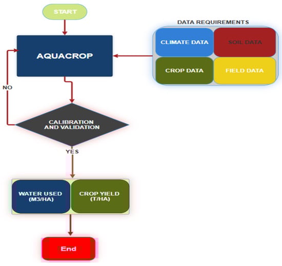
Figure 3. Schematic representation of the AquaCrop model.

For this study, AquaCrop was parameterized for rice (GRDB 10), maize, and soybean, and simulations were performed using observed weather data from 2014 to 2022 for calibration and validation, while simulated weather data were used to project crop performance for 2014–2025. Model inputs included daily rainfall, maximum and minimum temperatures, ETo, soil profiles, management practices, and CO² levels.

Biomass production in AquaCrop is based on normalized water productivity ($W{P}^{*}$) and crop transpiration, which is linked to ETo; yield is then calculated from the harvest index (HI) adjusted for water or temperature stress [42,43]. Full details of the AquaCrop algorithms are provided in the model documentation [43].

2.8.1. Soil Data and Irrigation

The dominant soil at Rose Hall Estate belongs to the Whittaker Series, 37, as documented by Steele [44]. This soil type covers approximately 45,800 acres (about 6.4% of the national area) and extends along the coast from Rose Hall Sugar Estate in the northwest to Number 51 Village in Leeds in the southeast. Key characteristics of the Whittaker soil are summarized in Table 1.

Table 1. Measured soil properties of Whittaker 37 soil series (n = 12 samples) [45].

Layer	Depth (cm)	Particle Size Distribution (%)			USDA Texture	Bulk Density ($\mathbf{g}{\mathbf{cm}}^3$)	Ksat (mm/day)
		Clay	Silt	Sand
1	0–22	63	35	2	Clay	1.23	237.6
2	22–65	65	32	3	Clay	1.29	129.6
3	65–100	66	32	2	Clay	0.94	79.2
4	100–141	45	45	10	Silty-Clay	1.11	984

Agricultural lands at Rose Hall Estate are irrigated primarily by the Canje River, which provides a reliable water source for crop production. For this study, rice yield simulations assumed basin irrigation with a fixed schedule of 50 mm every eight days.

2.8.2. Calibration and Validation

AquaCrop was calibrated and validated using weather data from 2014 to 2022. The calibration process relied on observed weather data from 2014 and 2015, while the validation phase used data from 2016 and 2022. However, due to the recent large-scale production of soybeans and corn in Guyana, relevant historical yield data for these crops during the simulation period was unavailable for validation. Consequently, validation was exclusively performed for rice simulations in the Rosehall area.

The calibration of AquaCrop focused on refining non-conservative parameters within the system. Its primary goal was to minimize key performance metrics such as root mean square error, mean absolute error, and mean absolute percentage error between simulated and observed yields while maintaining physiologically realistic crop growth behaviour. Additionally, the calibration and validation process expanded to specific crop cultivation locations. In the case of rice simulations in Rosehall, calibration used yield data obtained from the Blackbush Polder rice region (an area that is close to Rosehall), covering the May–June planting season from 2014 to 2022.

In the absence of corresponding historical yield data for corn and soy within this timeframe, calibration relied on research experiments conducted on these crops on clay soils.Wahab [46], Wahab and Hassan [47] focused their research on soybean yields across Guyana’s clay (Inki and Whittaker 37 series) and peat soils, demonstrating that optimal conditions, including adequate drainage, fertilizer application, and effective crop and soil management, led to favourable yields ranging from 2.0 to 2.4 t ha⁻¹ and reaching as high as 4.9 t ha⁻¹. Leveraging this valuable insight, AquaCrop underwent calibration in clay soils against these obtained yields. Meanwhile, Singh et al. [48], Moonilall et al. [49] investigated corn productivity under varying management and soil conditions, reporting yields ranging from 5.6 to 10.5 t ha⁻¹ under optimal conditions with proper spacing, drainage, and fertilization.

For soybean and corn, calibration focused on refining non-conservative parameters governing canopy development, rooting depth, and phenological timing to ensure model realism under Guyana’s agro-climatic conditions. For soybean, adjustments were made to the initial canopy cover (1.43%), maximum canopy cover (99%), canopy expansion period (65 days), flowering duration (62 days), and maximum rooting depth (0.6 m) until simulated yields under Whittaker clay soil stabilized between 2.0 and 2.4 t ha⁻¹, consistent with reported values [47]. For corn, the canopy development period (50 days), maximum canopy cover (90%), rooting depth (1 m), and harvest index (40%) were iteratively tuned to match reported yields of 5.6 to 10.5 t ha⁻¹ [48,49].

2.8.3. Planting Windows and Intervals

Table 2 and Table 3 display the planting windows, planting intervals, and corresponding planting dates for the crops used in the simulations. As the time during which these crops are planted can affect yields, the planting windows were subdivided into smaller intervals spanning 14–16 days. These smaller windows also facilitate better comparisons of yields obtained under observed and simulated weather conditions. The yield for a given planting interval was defined as the arithmetic mean of the simulated yields for the three distinct planting dates that define that interval.

Table 2. Planting intervals.

Planting Intervals	Planting Dates in Interval
15 May–30 May	M15, M23, M30
23 May–7 Jun	M23, M30, J7
30 May–15 Jun	$\mathrm{M}30,\mathrm{J}7,\mathrm{J}15$
7 Jun–23 Jun	$\mathrm{J}7,\mathrm{J}15,\mathrm{J}23$
15 Jun–30 Jun	$\mathrm{J}15,\mathrm{J}23,\mathrm{J}30$
15 Oct–30 Oct	$\mathrm{O}15, \mathrm{O}23, \mathrm{O}30$
23 Oct–7 Nov	$\mathrm{O}23, \mathrm{O}30, \mathrm{O}7$
30 Oct–15 Nov	$\mathrm{O}30,\mathrm{N}7,\mathrm{N}15$
7 Nov–23 Nov	$\mathrm{N}7,\mathrm{N}15,\mathrm{N}23$
15 Nov–30 Nov	$\mathrm{N}15,\mathrm{N}23,\mathrm{N}30$

Table 3. Planting windows.

Crop	Planting-Window	# of Intervals
Rice (irrigated)	15 May–30 Jun	5
Rice (rain-fed)	15 May–15 Jun	3
Soy	30 May–30 Jun	3
Corn	15 Oct–30 Nov	5

2.9. Multi-Objective Optimization

This study employs multi-objective optimization (MOO) to identify optimal crop planning strategies that balance competing goals, such as maximizing profit and water productivity while minimizing land use. A general MOO problem can be expressed as:

$$Max/Min\mathbf{U}\left(\mathbf{x}\right)={\left(U_1\left(\mathbf{x}\right),U_2\left(\mathbf{x}\right),\dots ,U_k\left(\mathbf{x}\right)\right)}^T,\mathbf{x}={(x_1,x_2,\dots ,x_n)}^T,$$

$$g_i\left(\mathbf{x}\right)\le h_i,i=1,2,\dots ,m,$$

where $U_j\left(\mathbf{x}\right)$ are the objective functions to be optimized simultaneously, $\mathbf{x}$ represents decision variables (e.g., crop choices, planting intervals), and $g_i\left(\mathbf{x}\right)$ are problem-specific constraints.

• Pareto-based Optimization:

A Pareto dominance approach was used to explore trade-offs between objectives [50,51]. In this approach, a solution ${\mathbf{x}}^{*}$ is Pareto optimal if no other feasible solution improves one objective without degrading another. The resulting Pareto front consists of all non-dominated solutions, offering decision-makers a range of trade-off options.

This framework provides a systematic way to evaluate cropping strategies under multiple constraints, ensuring that economic, agronomic, and environmental objectives are considered simultaneously.

Model Index and Parameters

• i: A crop which can be considered for production.
• j: A crop combination made up from i.
• l: A crop planting interval combination dependent upon j.
• n: The number of crops in a single combination determined by j.
• $Y_{ijkl}$: The average yield in metric tons of crop i in crop combination j for crop planting interval combination l.
• $P_{il}$: Export price per metric ton of crop i in crop planting interval combination l.
• $Q_{il}$: Local price per metric ton of crop i in crop planting interval combination l.
• $X_i$: The percentage of crop i to be exported.
• $P{C}_{ijl}$: Cost to produce 1 hectare of crop i in crop combination j for crop planting interval combination l.
• $EPR{T}_{ijl}$: Export profit obtained from producing 1 hectare of crop i in crop combination j for crop planting interval combination l$m.=\left(X_i\times P_{il}\times Y_{ijl}-P{C}_{ijl}\right)$.
• $DPR{T}_{ijl}$: Domestic profit obtained from producing 1 hectare of crop i in crop combination j for crop planting interval combination l, $.=\left(\left(1-X_i\right)\times P_{il}\times Y_{ijl}-P{C}_{ijl}\right)$.
• $E{T}_{ijl}$: Average evapotranspiration in cubic meters per hectare of crop i, in crop combination j for crop planting interval combination l.
• $D_i$: Demand for crop i in metric tons of crop land.
• L: The amount of land in hectares.
• TI: Total investment.
• TD: Total demand.

• Decision variable

$A_{ijl}$: The area of land in hectares to be cultivated for crop i in crop combination $\mathrm{j}$ for crop planting interval combination l.

2.10. Multi-Objective Optimization Model

The multi-objective optimization (MOO) framework was designed to determine optimal crop planning strategies by balancing three competing objectives: (i) maximizing gross profit, (ii) maximizing evapotranspiration (ET) economic water productivity, and (iii) minimizing total land use. These objectives and constraints are defined as follows.

Objectives:

• Maximize gross profit:
  Profit is computed as the total revenue minus production costs across all crops, planting dates, and land units:

  $$\mathrm{Profit}=\sum _{i=1}^k{\mathrm{EPRT}}_{ijl}·A_{ijl}+\sum _{i=1}^k{\mathrm{DPRT}}_{ijl}·A_{ijl},$$

  (23)

  where ${\mathrm{EPRT}}_{ijl}$ and ${\mathrm{DPRT}}_{ijl}$ are early and delayed planting revenue per hectare, and $A_{ijl}$ is the allocated area for crop i in location j at planting time l.
• Maximize ET economic water productivity:
  This metric reflects the economic return per unit of crop water use:

  $$\mathrm{ET}\mathrm{economic}\mathrm{water}\mathrm{productivity}=\sum _{i=1}^n{\displaystyle \frac{\mathrm{Profit}}{E{T}_{ijl}·A_{ijl}}},$$

  (24)

  where $E{T}_{ijl}$ is the total evapotranspiration for crop i in location j at planting time l.
• Minimize land use:
  To promote efficient resource allocation, total cultivated area is minimized as follows:

  $$\mathrm{Land}\mathrm{use}=\sum _{i=1}^n{A}_{ijl}.$$

  (25)

Constraints:

• Investment constraint:
  Total production costs must not exceed the available investment budget ($\mathrm{TI}$):

  $$\sum _{i=1}^{n}P{C}_{ijl}·A_{ijl}\le \mathrm{TI}.$$

  (26)
• Land constraint:
  The cultivated area per region cannot exceed the available land ($L_k$):

  $$\sum _{i=1}^n{W}_k·A_{ijl}\le L_k,\forall k,$$

  (27)

  where $W_k=1$ for monoculture and $W_k=0.5$ for double cropping.
• Demand constraint:
  Total yield must meet or exceed a target production level (T):

  $$\sum _{i=1}^k{Y}_{ijl}·A_{ijl}\ge T.$$

  (28)

This formulation enables the exploration of trade-offs between profit, water productivity, and land use, generating Pareto-optimal solutions to guide decision-making.

2.10.1. Domestic and Export Prices

The export prices used in the study for simulation were obtained from the World Bank commodity prices database. To forecast prices for 2024, the R package auto. arima (version 2022.02.4+500) was employed to derive ARIMA models for forecasting international rice, corn, and soy prices on Monthly data from January 1988 to March 2024. The auto. arima function in R applies a modified version of the Hyndman-Khandakar method, which incorporates unit root testing, AICc minimization, and maximum likelihood estimation to formulate an ARIMA model [52]. Following data assimilation, the optimal ARIMA models for forecasting were determined to be ARIMA (1,1,2), ARIMA (2,1,2), and ARIMA (2,1,3) for rice, soy, and corn, respectively. Price projections were made for 14 months extending to May 2025.

Only two years’ worth of domestic pricing data were available for each crop, which was derived from local market data (rice) and feasibility studies conducted by organizations such as NAREI for soy and corn (see Appendix A). A conversion rate of GYD 204 = USD 1 was consistently applied throughout the study. As domestic prices (like international prices) fluctuate over time, it is imperative to integrate fluctuating costs into the optimization model for a more realistic representation. Due to limited data, achieving dynamic domestic pricing necessitated an assumption of fixed price changes. This involved calculating the difference between prices and dividing the result by the number of months between data collection periods to achieve a fixed value. This fixed value was added to domestic prices on a monthly basis to create non-stationary price changes. To maintain consistency in how the dynamic pricing data for export and production costs are determined, all prices provided are assumed to represent year-end prices. The formula used to achieve dynamic pricing can be seen below.

Let $P_{\mathrm{start}}$ and $P_{\mathrm{end}}$ denote the domestic prices observed at two data collection points separated by M months. The fixed monthly change $\Delta P$ was computed as follows:

$$\Delta P={\displaystyle \frac{P_{\mathrm{end}}-P_{\mathrm{start}}}{M}}.$$

The dynamic monthly domestic price series was then generated as follows:

$$P_t=P_{\mathrm{start}}+t\Delta P,t=0,1,\dots ,M,$$

so that prices evolve linearly over time while remaining consistent with the observed endpoints. Having defined the approach for dynamic price generation, it was also necessary to account for temporal variations in production costs, since the profitability objectives depends jointly on both price and cost behaviour.

2.10.2. Production Cost Estimates

Local production cost data were only available for rice (four years) and corn (one year), respectively. To establish dynamic production cost data for rice over time, a similar approach to that used for domestic pricing was employed. Given that only one year of corn and no years’ worth of soybean production data were available, Iowa State’s historical cost of production data were used. To convert these prices to ones suitable for use in Guyana, the cost of producing 1 hectare of corn along Guyana’s coast (of which Rose Hall is a part) in 2013 was compared to the cost of producing 1 hectare of corn in Iowa in 2013. It was then deduced that the cost of producing 1 hectare of corn on the coast was approximately $67.72\%$ of the cost of producing the same hectare in Iowa. Since the Iowa dataset provided historical yearly average production costs from 1975 to 2024 for both corn and soybeans, the estimated $67.72\%$ cost of production was used to estimate costs for both crops (Appendix A). Since the data were collected on a yearly time frame, the same procedure used for determining domestic pricing was applied.

The milling cost for rice was estimated to be about USD 49 per ton, with a paddy-to-mill rice conversion rate of $0.65\%$. The cost for drying corn and soybeans was estimated to be USD 25 and USD 20, respectively.

With both the price and production cost components established, the next step was to formulate the complete optimization model, integrating these economic variables with the agronomic data and hydrological constraints described earlier.

2.10.3. Model Description

This multi-objective optimization model aims to determine the optimal amount of land to allocate for various crop-planting interval combinations (for polyculture, sequential double cropping, triple cropping, and N-cropping) that simultaneously optimize model objectives. Considering the study location, climatic conditions, soil types, and the crops used for modeling, simulations are limited to sequential double cropping only.

In this system, two crops are cultivated on the same land within a single year, one right after the other’s harvest. Within the optimization model, the decision variable $A_{ijl}$ represents the area of land (in hectares) allocated to crop i in crop combination j for planting interval l. The land constraint includes a proportional coefficient $W_k$, which scales total land use according to the cropping system. For sequential double cropping, $W_k=0.5$, ensuring that the combined annual land use of both crops does not exceed the available physical area. Because the same land is used sequentially rather than simultaneously, a nominal total of 5000 ha was used in the simulations to represent the potential sequential use of 2500 ha within a single production year. This adjustment preserves the integrity of the land-use constraint while allowing both crops to be optimized across their planting intervals.

The crops used for simulations have several potential planting intervals, each approximately two weeks wide (Appendix A). Upon initiation, the model first determines whether simulations will be conducted for polyculture or sequential double cropping. Following this determination, the appropriate cropping combination mix is identified based on the chosen cropping method. For instance, the model identifies suitable cropping combinations when sequential double cropping is selected. For this research, the double cropping combinations are rice and corn and soy and corn. Each of these crops has M, N, and O planting intervals, which generate $M\times O$ and $N\times O$ possible combinations. The model finds these individual combinations and runs the multi-objective optimization for each, generating $(M\times O)+(N\times O)$ different Pareto fronts. Each Pareto front comprises the optimal land sizes (the decision variable) necessary to optimize all three objectives for a specific crop combination, subject to the defined constraints. This separation allows for the comparison of different crop combinations and enables specific objectives to be isolated; for example, identifying the crop interval combination that yields the highest profit or the greatest ET economic water productivity.

2.11. NSGA-II Algorithm

The Non-dominated Sorting Genetic Algorithm II (NSGA-II) is a second-generation multi-objective evolutionary algorithm (MOEA) developed by Deb et al. [53]. It improves upon the original NSGA through a more efficient non-dominated sorting procedure, removal of the sharing parameter, and the introduction of an elitist selection mechanism, all of which enhance convergence toward the Pareto-optimal front [53,54]. In NSGA-II, candidate solutions are ranked based on non-domination levels, and a crowding distance metric is applied to preserve diversity. A binary tournament selection is then performed, prioritizing solutions with lower rank and greater diversity [53,55]. This algorithm was chosen for the present study due to its proven effectiveness in crop planning and agricultural optimization problems [19,54]. Parameter settings were based on recommendations from the literature [19,54,56], with a crossover probability of $P_c=0.9$, a mutation probability of $P_m=1/DV$ (where $DV$ is the number of decision variables), a population size of $N=200$ (within the recommended range of 100–300), and distribution indices of $C{D}_i=20$ and $M{D}_i=20$ for crossover and mutation, respectively.

2.12. Simulation Scenarios and Interval Overlaps

This study includes four simulation scenarios for the 2024/25 crop season, conducted over 2500 hectares of farmland, with a focus on export targets of approximately 25% and 50% of total crop production. To address overlapping planting intervals, results from the earlier interval are used when dates intersect. For example, the planting windows from 15 May–30 May and 22 May–7 June overlap between 22 May–30 May; in such cases, outcomes from the 15 May–30 May interval are applied to ensure consistency in interpreting results.

Performance Metrics

The performance of the temperature and relative humidity models was assessed using summary statistics as well as the RMSE (root mean square), MAE (mean absolute error), and MAPE (mean absolute percentage error). Performance assessment of the ANN model for ETo estimation was carried out using RSME, MAE, $R^2$ (coefficient of determination), and a regression coefficient-based method given by Equation (29) [57,58].

$${\mathrm{ET}}_{ES}=\mathrm{A}·{\mathrm{ET}}_{\mathrm{P}\mathrm{M}56}+\mathrm{B}$$

(29)

where A is the regression gradient, and B is the intercept. A and B values closer to unity and zero are deemed optimal [58].

3. Results

3.1. Results of Precipitation Simulation

Analysis of the transition probability matrices (Table 4) reveals seasonal rainfall patterns at Rose Hall consistent with Guyana’s established bimodal precipitation regime [59]. May and June exhibited the lowest probability of transitioning from a wet to a dry day ($p_{wd}<0.4$), aligning with the onset of the primary rainy season. These months, along with July, showed the highest likelihood of consecutive wet days ($p_{ww}>0.5$), indicating persistent rainfall events. In contrast, January and February recorded the highest wet-to-dry day transition probabilities ($p_{wd}\ge 0.6$), marking the mid-dry season.

Table 4. Transition probability matrix for Rose Hall (1981–2022).

State	Dry	Wet	Month	State	Dry	Wet	Month
Dry	0.836	0.164	Jan	Dry	0.565	0.435	Jul
Wet	0.607	0.393		Wet	0.463	0.537
Dry	0.829	0.171	Feb	Dry	0.666	0.334	Aug
Wet	0.619	0.381		Wet	0.502	0.498
Dry	0.858	0.142	Mar	Dry	0.776	0.225	Sep
Wet	0.573	0.427		Wet	0.612	0.388
Dry	0.827	0.173	Apr	Dry	0.774	0.226	Oct
Wet	0.513	0.487		Wet	0.594	0.406
Dry	0.669	0.331	May	Dry	0.791	0.209	Nov
Wet	0.396	0.604		Wet	0.549	0.451
Dry	0.526	0.474	Jun	Dry	0.796	0.204	Dec
Wet	0.392	0.608		Wet	0.557	0.443

Overall, the probability of transitioning from a dry to a wet day was consistently lower than that of consecutive wet days ($p_{dw}<{\pi }_w<p_{ww}$), confirming seasonal rainfall persistence [60].

3.1.1. Steady-State Probabilities and Rainfall Regime

The steady-state vectors derived from the Markov chains (Table 5) quantify the long-term probabilities of wet and dry conditions. May, June, and July each exhibited wet-day probabilities exceeding 0.45, with June showing the highest (0.61), corresponding to the peak rainy season. Conversely, September through November were characterized by lower wet-day probabilities (<$0.28$), reflecting Guyana’s dry season.

Table 5. Steady-state probability vectors for wet and dry days at Rose Hall (1981–2022).

Jan	Feb	Mar	Apr
$[0.788,0.212]$	$[0.783,0.217]$	$[0.801,0.199]$	$[0.748,0.252]$
May	Jun	Jul	Aug
$[0.545,0.456]$	$[0.392,0.608]$	$[0.516,0.484]$	$[0.600,0.400]$
Sep	Oct	Nov	Dec
$[0.732,0.268]$	$[0.725,0.275]$	$[0.724,0.276]$	$[0.732,0.268]$

3.1.2. Monthly Rainfall Distribution

Descriptive statistics from 1981 to 2022 (Appendix A) highlight pronounced variability in monthly rainfall. The primary rainy season extended from May through July, while September–November marked a relatively dry period. October recorded the lowest mean rainfall per wet day (8.96 mm) and the lowest maximum daily rainfall (48.93 mm), while January exhibited the highest maximum daily rainfall (233.02 mm). The number of wet days also varied, ranging from only 257 in February to over 600 in June and July. Interestingly, months with fewer rainy days, such as December and January, tended to have heavier rainfall on those days, reinforcing the need for month-specific probability distribution fitting.

3.2. Distribution Fitting and Precipitation Simulation

• Distribution parameter estimation and selection

Maximum Likelihood Estimation (MLE) was used to estimate parameters for all candidate distributions, with the best-fitting models for each month identified using Akaike Information Criterion (AIC) values and Probability–Probability (PP) plots. Distributions with the lowest AIC values and PP plots that closely aligned with the reference line were selected as optimal fits. Table 6 summarizes the chosen distributions, parameter estimates, and corresponding AIC values. Fits were generally strong across most months, although January and February achieved only moderate fits, requiring additional simulation iterations to align with observed patterns. Full PP plots for all months are provided in Appendix A.

Table 6. Best-fitting probability distributions, parameter estimates, and AIC values by month.

Month	Distribution	Loc	Shape	Scale	Threshold	AIC
Jan	Lognormal	2.667	–	1.002	–	2260.7
Feb	Lognormal	2.491	–	0.784	–	1889.0
Mar	Gamma	–	0.687	23.62	–	1944.7
Apr	Gamma	–	2.043	9.687	–	2460.8
May	Gamma (3p)	–	1.879	9.000	1.562	4436.6
Jun	Gamma	–	2.297	7.577	–	5115.2
Jul	Lognormal	2.730	–	0.660	–	4708.2
Aug	Lognormal	2.624	–	0.636	–	3738.8
Sep	Gamma	–	2.432	4.736	–	2212.4
Oct	Gamma (3p)	–	1.746	4.966	0.285	2211.9
Nov	Lognormal	2.482	–	0.718	–	2488.5
Dec	Lognormal	2.746	–	0.828	–	2780.7

Loc = Location, Scale = Sc, Threshold = Th.

• Simulation of precipitation occurrence and amounts

The calibrated first-order Markov chain model was used to simulate precipitation occurrence over a 50-year period (1981–2030). Simulated results for 1981–2022 closely matched observed values (Table 7), with strong agreement in most months. May through July and November showed particularly high simulation accuracy, confirming the model’s ability to replicate seasonal rainfall persistence.

Table 7. Observed vs. simulated monthly precipitation occurrence (wet days) at Rose Hall (1981–2022).

Month	Observed	Simulated
Jan	276	282
Feb	257	265
Mar	260	261
Apr	318	315
May	594	603
Jun	691	699
Jul	631	626
Aug	520	527
Sep	338	335
Oct	358	345
Nov	348	340
Dec	350	360

Comparison of simulated and observed precipitation amounts shows strong agreement in central tendencies, with similar means, medians, and quartile ranges, while some discrepancies were observed in extreme values—likely due to outliers or model limitations, the quartile spread indicates that the model reliably captures typical precipitation patterns (Appendix A). Overall, the precipitation model demonstrates high fidelity in replicating observed seasonal rainfall characteristics, supporting its use for forward-looking simulations.

• Projections for 2023–2030

Using the same calibrated model, precipitation was simulated for 2023–2030. Seasonal patterns remained consistent with historical data, with May, June, and July recording the highest number of wet days (138, 150, and 126, respectively). September and October continued to exhibit the lowest rainfall frequency. Some months showed lower average precipitation per wet day than the historical period, although December, January, and April remained relatively high, reflecting observed trends. January also retained the highest variability, with a standard deviation of 24.58. Differences in simulated mean precipitation for January, February, and April highlight areas where further refinement may enhance long-term projections.

3.3. Stochastic Differential Equation (SDE) Model for Temperature and Relative Humidity

• Parameter estimation

Attempts to estimate Ornstein–Uhlenbeck (O–U) parameters for minimum and maximum temperature by month were unsuccessful, likely due to limited variability in monthly data. Instead, parameters were estimated using the full dataset (2001–2020). As shown in Table 8, the minimum temperature exhibited higher volatility ($\gamma =1.0563$) and a faster mean reversion rate ($\lambda =0.5764$) than the maximum temperature, suggesting quicker stabilization around its long-term mean. Seasonal variations were not explicitly captured due to the inability to parameterize the SDE model at the monthly level. For simulation, the annual values of $\lambda$, $\mu$, and $\gamma$ from Table 8 were applied uniformly throughout the simulation period. The inability to compute monthly parameters likely resulted from the small inter-month temperature differences observed in Guyana (approximately 3 °C between the warmest and coolest months), which provided insufficient variability for reliable estimation.

Table 8. SDE parameters for maximum and minimum temperature (2001–2020). Minimum temperatures revert faster and show greater volatility.

Temperature	$\mathsf{\mu }$	$\mathsf{\lambda }$	$\mathsf{\gamma }$
Maximum	31.406	0.4573	1.0066
Minimum	23.611	0.5764	1.0563

For relative humidity, parameters were successfully derived for each month (Table 9). Humidity showed distinct seasonality, with mean values ranging from 74.17% in October to 81.66% in June. The highest mean reversion speeds ($\lambda >13$) and volatility ($\gamma >9$) were recorded in June, July, and August, reflecting greater variability during the mid-year rainy season. For simulation, the corresponding monthly values of $\lambda$, $\mu$, and $\gamma$ from Table 9 were applied according to the simulated day of the year, allowing the model to represent both the seasonal and stochastic behavior of humidity.

Table 9. Monthly SDE parameters for relative humidity (2001–2020). Highest variability observed in June–August.

Month	$\mathsf{\mu }$	$\mathsf{\lambda }$	$\mathsf{\gamma }$
Jan	77.82	0.62	5.42
Feb	77.14	0.79	6.14
Mar	75.53	0.58	5.02
Apr	77.07	0.70	5.67
May	80.61	1.99	8.49
Jun	81.66	13.82	15.97
Jul	80.69	13.19	12.29
Aug	78.49	12.22	9.63
Sep	75.71	2.05	6.60
Oct	74.17	1.45	6.83
Nov	76.07	1.27	6.94
Dec	79.36	0.83	6.65

• Model validation

Simulated temperature and humidity were compared with observed data (Table 10 and Table 11). The O–U model reproduced the statistical properties of both variables, with strong agreement in mean and median values. Quartile spreads were consistent, indicating the model’s reliability in capturing central tendencies. However, some underestimation of extreme values was observed, particularly for maximum temperatures and humidity extremes, suggesting a limitation in modeling tails of the distributions.

Table 10. Simulated vs. observed temperature summary statistics (2001–2020).

Metric	Sim (Max)	Sim (Min)	Obs (Max)	Obs (Min)
Mean	31.37	23.58	31.39	23.60
Median	31.37	23.60	31.40	23.70
Std Dev	1.06	0.99	1.44	1.24
Min	27.51	19.15	24.10	15.10
Max	34.95	28.09	36.20	26.80
Q1	30.64	22.92	30.50	22.90
Q3	31.37	23.60	31.40	23.70

Table 11. Simulated vs. observed relative humidity summary statistics (2001–2020).

Metric	Observed	Simulated
Mean	77.68	77.94
Median	77.81	78.00
Std Dev	6.06	4.61
Min	56.25	60.00
Max	103.91	96.00
Q1	73.75	75.00
Q3	81.42	81.00

Figure 4 and Figure 5 show time–series comparisons of observed and simulated values for 2015–2020, confirming the model’s ability to reproduce variability patterns.

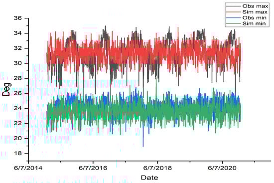
Figure 4. Observed vs. simulated minimum and maximum temperatures at New Amsterdam (2015–2020).

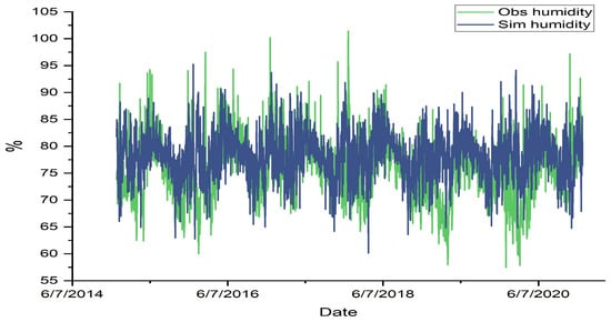
Figure 5. Observed vs. simulated relative humidity at New Amsterdam (2015–2020).

• Future simulations (2021–2030)

The SDE model was applied to simulate temperature and humidity for 2021–2030. Model performance was validated for 2021–2022 using MAE, RMSE, and MAPE, all of which indicated strong agreement. RMSE and MAE remained below 1.9 and 1.5, respectively, for temperature, while humidity RMSE remained under 7%. Projections for 2023–2030 showed similar statistical patterns, reinforcing the model’s reliability for medium-term forecasting.

3.4. ETo Estimation

Daily reference evapotranspiration (ETo) was estimated for New Amsterdam between 2019 and 2022 using the PM-56 method. During this period, daily ETo values ranged from 1.71 mm (15 January 2021) to 6.34 mm (3 March 2020), with an overall mean of 4.57 mm day⁻¹ and a standard deviation of 0.69 mm. August and September consistently recorded the highest monthly averages, reflecting Guyana’s peak warm period, while January and February had the lowest mean ETo values.

The Artificial Neural Network (ANN) model was trained on historical data and tested on previously unseen data from 2019 to 2022. Evaluation metrics confirmed excellent performance, with RMSE and MAE values of 0.1373 mm and 0.123 mm, respectively, and a coefficient of determination ($R^2$) of 98.76%. Regression coefficients were $A=0.99$ and $B=0.161$, indicating a near 1:1 relationship between ANN predictions and PM-56 estimates. The ANN accurately captured the distribution of ETo, with a mean of 4.68 mm, a standard deviation of 0.68 mm, and a maximum of 6.28 mm, closely matching PM-56 results (Figure 6).

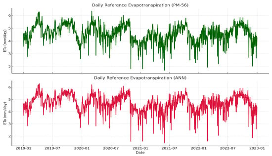
Figure 6. Comparison of daily ETo estimates by PM-56 and ANN for New Amsterdam (2019–2022).

ETo Simulation Using Weather Model Data

The trained ANN model was then coupled with simulated weather inputs: minimum and maximum temperatures, relative humidity, and solar radiation (computed using Equation (27)), to produce ETo estimates. Simulated values for 2019–2022 demonstrated strong alignment with PM-56 results, with summary statistics showing a mean of 4.59 mm day⁻¹, a standard deviation of 0.46 mm, and a range of 2.92–5.97 mm. Time-series comparisons (Figure 7) confirm that the weather-driven ANN model successfully reproduces temporal variability in ETo, validating its utility for subsequent crop growth simulations.

Figure 7. Time series comparison of simulated ANN-derived ETo and PM-56 estimates (2019–2022).

3.5. Crop Yield Simulations Using AquaCrop

3.5.1. Observed and Simulated Climatic Conditions

The observed monthly maximum and minimum temperatures at Rose Hall remained relatively stable during the testing period, ranging from 30.73 °C to 33.28 °C for maximum and 24.41 °C to 24.74 °C for minimum temperatures. Observed precipitation averaged $204.15\mathrm{mm}$ per month, while daily reference evapotranspiration (ETo) averaged $4.69\mathrm{mm}$.

Simulated climate variables closely matched observed conditions. Simulated maximum and minimum temperatures ranged from 31.17 °C to 31.60 °C and 23.49 °C to 23.74 °C, respectively. Simulated precipitation averaged $206\mathrm{mm}$ per month, with daily ETo of $4.61\mathrm{mm}$.

3.5.2. Calibration and Validation of AquaCrop Yields

Calibration of AquaCrop parameters was performed using observed field data (2014–2017) and weather records, supplemented with published data sources [61,62,63] and local farmer records. Calibrated parameters resulted in at least $90\%$ maximum canopy cover and a harvest index above $36\%$ for all crops.

Following calibration, AquaCrop accurately reproduced irrigated rice yields using both observed and simulated climate data. The Root Mean Square Error (RMSE) was below $0.65\mathrm{t}/\mathrm{ha}$, and the Mean Absolute Percentage Error (MAPE) remained under $8\%$. Average yearly yields were computed by averaging across planting dates within the designated planting window. Table 12 presents the performance metrics for the calibration period (2014–2017).

Table 12. Performance metrics of yield simulations after calibration for 15 May–30 June window.

Year	Yield (ton/ha)			RMSE (ton/ha)		MAE	MAPE %
	2014	2015	2016	2017
Actual	6.1	6	5.2	5.9
Obs wthr	6.11	6.22	6.35	6.45	0.642	0.478	7.518
Sim wthr	6.27	6.27	6.38	6.445	0.618	0.456	7.237

Obs wthr = simulations using observed weather; Sim wthr = simulations using simulated weather.

Validation was performed for 2018–2022 using both observed and simulated weather data. Results demonstrate strong agreement between predicted and actual irrigated rice yields, confirming that simulated climate data can reliably reproduce historical yield trends. Validation data are presented in Table 13 and Table 14.

Table 13. Yield simulations from 2018 to 2022 (observed vs. simulated weather).

	Yield (ton/ha)
Year	2018	2019	2020	2021	2022
Actual	6.55	6.8	6.1	6	6.3
Obs wthr	6.45	6.42	6.39	6.55	6.59
Sim wthr	6.35	6.49	6.52	6.55	6.53

Table 14. Performance metrics for yield simulations from 2018 to 2022.

RMSE	MAE	MAPE
0.32	0.282	4.35
0.312	0.29	4.49

3.5.3. Simulated and Projected Yields for All Crops (2014–2025)

Following calibration and validation, AquaCrop was applied to simulate yields for irrigated rice, rain-fed rice, soybeans, and maize across all planting intervals, integrating both observed and model-generated weather inputs (Appendix C). Under observed weather conditions, yields were generally stable, with irrigated rice consistently achieving $5.9$–$6.6\mathrm{t}{\mathrm{ha}}^{-1}$, rain-fed rice $5.2$–$6.7\mathrm{t}{\mathrm{ha}}^{-1}$, soybeans $2.1$–$3.3\mathrm{t}{\mathrm{ha}}^{-1}$, and maize $7.7$–$10.0\mathrm{t}{\mathrm{ha}}^{-1}$.

Performance evaluation showed strong model fidelity for irrigated rice, where predictions under simulated weather closely mirrored observed-weather results (MAPE $<3\%$, RMSE $<0.21\mathrm{t}{\mathrm{ha}}^{-1}$). rain-fed rice yields were also reliable, though slightly more variable (MAPE up to $8.6\%$), while maize simulations exhibited similarly strong alignment (MAPE 6–$9.6\%$). Soybean simulations were moderately accurate (MAPE 10–$13\%$), reflecting the crop’s sensitivity to rainfall and seasonal variability, as also noted in similar studies.

Average annual yields aggregated across all planting intervals revealed modest to good agreement between values simulated under model-generated weather and those produced using observed weather data (Figure 8 and Figure 9) for rice. For irrigated rice, yields under simulated weather ranged from $6.3$–$6.6\mathrm{t}{\mathrm{ha}}^{-1}$, while those under observed weather varied between $6.2$–$6.6\mathrm{t}{\mathrm{ha}}^{-1}$, reflecting less than $5\%$ interannual deviation. Rain-fed rice exhibited lesser stability, with simulated yields between $6.0$–$6.5\mathrm{t}{\mathrm{ha}}^{-1}$ and observed yields between $5.9$–$6.6\mathrm{t}{\mathrm{ha}}^{-1}$, though the latter displayed slightly greater sensitivity to rainfall variation during 2015–2019.

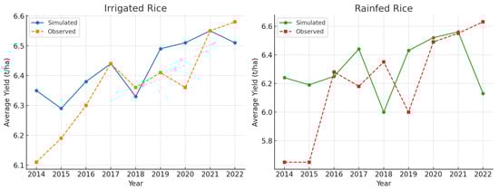
Figure 8. Comparison between irrigated and rain-fed rice yields under simulated and observed weather conditions at Rose Hall. Simulated and observed yields exhibit close agreement, confirming the robustness of the AquaCrop simulations across planting intervals (2014–2022).

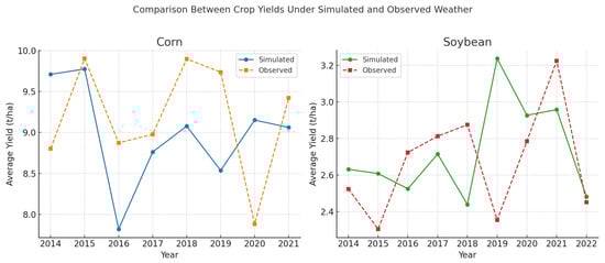
Figure 9. Comparison between maize and soybean yields under simulated and observed weather conditions at Rose Hall. Both crops show good agreement between simulated and observed values, with minor deviations attributed to rainfall sensitivity and planting date variability.

For maize, simulated yearly average yields fluctuated between $8.0$–$9.5\mathrm{t}{\mathrm{ha}}^{-1}$, while observed yields ranged from $8.5$–$9.9\mathrm{t}{\mathrm{ha}}^{-1}$. The strongest correspondence occurred in 2015–2018, where both datasets followed close year-to-year patterns. Over the years, soybean yields averaged $2.6$–$3.2\mathrm{t}{\mathrm{ha}}^{-1}$ under simulated weather and $2.5$–$3.2\mathrm{t}{\mathrm{ha}}^{-1}$ under observed weather, with the largest divergence occurring in 2018–2019 due to rainfall anomalies captured by the AquaCrop model. Overall, the simulated and observed series tracked each other well across all crops and years, maintaining some interannual trends and magnitudes. This consistency highlights the robustness of the ANN–AquaCrop framework in reproducing annual yield dynamics under both historical and stochastically generated climatic conditions.

Projections for 2023–2025, based on weather simulations, indicate that rice yields should remain relatively stable, with irrigated rice projected between $6.51$–$6.64\mathrm{t}{\mathrm{ha}}^{-1}$ and rain-fed rice between $6.08$–$6.62\mathrm{t}{\mathrm{ha}}^{-1}$. Maize is expected to yield $7.5$–$10.1\mathrm{t}{\mathrm{ha}}^{-1}$, while soybeans maintain $2.1$–$3.3\mathrm{t}{\mathrm{ha}}^{-1}$. These findings demonstrate AquaCrop’s robustness as part of the broader modeling framework, which links stochastic weather simulations, ETo estimation, and crop modeling to generate actionable insights.

3.6. Multi-Objective Optimization: Simulation Scenarios and Constraint Settings

The multi-objective optimization (MOO) model was applied to identify optimal double-cropping strategies that maximize gross profit, improve evapotranspiration-based economic water productivity (EEWP), and ensure efficient land use under production and investment constraints. Demand constraints were fixed at 4000 t of rice, 2000 t of soybeans, and 7000 t of maize, while investment constraints were defined as the total variable costs of all selected crop combinations plus a USD 10,000 buffer. Simulations explored two double-cropping systems: (1) rain-fed rice with corn or soybeans and (2) irrigated rice with corn or soybeans, with soybeans grown exclusively under rain-fed conditions.

A total of 70 double-cropping combinations were evaluated (40 for irrigated systems and 30 for rain-fed systems), each producing its own Pareto front. These fronts illustrate trade-offs between maximizing profit and optimizing EEWP. Figure 10 and Figure 11 show representative Pareto fronts for rain-fed and irrigated rice systems, demonstrating non-dominated solutions where improvement in one objective comes at the expense of the other. These results provide decision-makers with a portfolio of viable solutions tailored to their priorities and constraints.

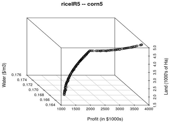
Figure 10. Pareto optimal front for double-cropping irrigated rice (Interval 1) and corn (Interval 5) under 25% export scenario.

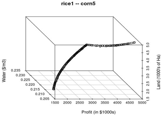
Figure 11. Pareto optimal front for double-cropping rain-fed rice (Interval 1) and corn (Interval 5) under 25% export scenario.

3.7. Optimal Double-Cropping Strategies Under 25% Export Scenario

Under the baseline assumption of 25% exports of rice, corn, and soybeans, double-cropping systems demonstrated strong profitability and high water-use efficiency, especially for rain-fed rice. The combination of rain-fed rice planted 15–30 May 2024 and corn planted 15–30 November 2024 generated the highest projected gross profit of USD 4,788,175 and an EEWP of USD 0.208 per m³ of water (Table 15). In contrast, the least profitable combination, soy, was planted 1–15 June and corn planted 15–30 October, yielded USD 2,214,882 (EEWP: USD 0.101 per m³), a reduction of 53.7% compared to the top-performing system. These results highlight the superior profitability of rice-corn rotations relative to soy-corn systems.

Table 15. Top five and bottom five double-cropping combinations with rain-fed rice for 2024/25 (25% export scenario).

Crop 1	Crop 2	Area 1	Area 2	Profit	EWP
rice1	corn5	2500	2500	4788.175	0.208
rice2	corn5	2500	2500	4732.885	0.205
rice3	corn5	2500	2500	4648.740	0.202
rice1	corn4	2500	2500	4621.205	0.199
rice2	corn4	2500	2500	4565.914	0.197
soy2	corn1	2500	2500	2454.721	0.109
soy1	corn4	2500	2500	2427.223	0.114
soy1	corn3	2500	2500	2353.372	0.109
soy1	corn2	2500	2500	2251.659	0.103
soy1	corn1	2500	2500	2214.882	0.101

For irrigated rice, the most profitable schedule involved planting rice 15–30 June and corn 15–30 November, producing USD 3,874,280 (EEWP: USD 0.165 per m³). Although this represents a 19.1% decrease compared to rain-fed rice under optimal conditions, irrigated systems provide stability and resilience in the face of rainfall uncertainty. Table 15 and Table 16 and Figure 12 and Figure 13, summarizes the five best- and worst-performing combinations for both systems, illustrating that top-performing strategies consistently feature early rice planting and late corn planting, while soybeans show greater variability and lower profitability.

Table 16. Top five and bottom five double-cropping combinations with irrigated rice for 2024/25 (25% export scenario).

Crop 1	Crop 2	Area 1	Area 2	Profit	EWP
riceIR5	corn5	2500	2500	3874.280	0.165
riceIR1	corn5	2500	2500	3834.000	0.165
riceIR4	corn5	2500	2500	3803.716	0.163
riceIR3	corn5	2500	2500	3784.442	0.165
riceIR2	corn5	2500	2500	3783.737	0.163
soy2	corn1	2500	2500	2454.721	0.109
soy1	corn4	2500	2500	2427.223	0.114
soy1	corn3	2500	2500	2353.372	0.109
soy1	corn2	2500	2500	2251.659	0.103
soy1	corn1	2500	2500	2214.882	0.101

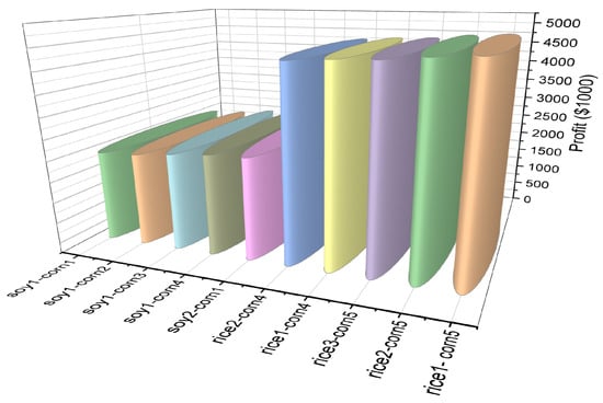
Figure 12. Best and worst-performing double-crop combinations with rain-fed rice under 25% export scenario.

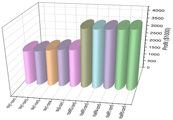
Figure 13. Best and worst-performing double-crop combinations with irrigated rice under 25% export scenario.

3.8. Sensitivity Analysis Under 50% Export Scenario

When exports were increased to 50% of total production, profits declined across all crop combinations due to lower projected export prices relative to domestic prices. For rain-fed rice, the top combination (rice: 15–30 May; corn: 15–30 November) yielded USD 4,216,054, a 12% reduction from the baseline scenario, while the least profitable soybean–corn combination fell to USD 1,505,402, a 32% drop. EEWP decreased correspondingly, with values ranging from USD 0.183 per m³ (best case) to USD 0.069 per m³ (worst case).

Irrigated rice combinations displayed a similar trend, with the highest-performing strategy (rice: 15–30 June; corn: 15–30 November) decreasing from USD 3,874,280 to USD 3,282,160, a 15.3% decline. The consistent ranking of crop-interval combinations across both export scenarios demonstrates the robustness of optimal planting schedules while highlighting the significant influence of market conditions on profitability. These results emphasize the utility of MOO frameworks for testing agricultural planning scenarios under fluctuating prices, land availability, and export targets.

4. Discussion

4.1. Integrating Dynamic Simulations and Optimization for Agricultural Planning

The modeling framework developed combined stochastic weather simulation, a process-based crop growth simulator, and multi-objective optimization (MOO) to guide agricultural decision-making in Guyana. Unlike traditional approaches that rely on static historical yield data or deterministic climate assumptions, our model uses dynamically simulated weather variables to drive crop yield estimation, resulting in a system that is both predictive and adaptable to future climate variability. The integration of a first-order Markov chain for precipitation occurrence, Ornstein–Uhlenbeck (O–U) stochastic differential equations for temperature and relative humidity, and an artificial neural network (ANN) for reference evapotranspiration (ETo) provides a robust foundation for simulating site-specific agro-climatic conditions. When combined with the FAO AquaCrop model, these simulations enable time-sensitive, location-specific crop yield estimates, capturing inter-annual variability and seasonal patterns that are essential for realistic agricultural planning.

This integration represents a significant advancement over prior agricultural planning models, many of which used static or aggregated yield statistics from national surveys, field trials, or literature values [19,64]. While these earlier works provided valuable insights into crop mix optimization and resource allocation, they often lacked the ability to represent weather-driven variability, limiting their predictive utility in regions like Guyana, where seasonal climate patterns strongly influence agricultural productivity. By contrast, this research leverages dynamic simulations to generate scenario-based yield predictions, thereby making the optimization component of the model responsive to changing environmental and economic conditions. Additionally, this approach captures temporal variability in weather patterns, such as fluctuations in rainfall distribution or shifts in evapotranspiration rates, which deterministic models cannot easily incorporate.

Beyond its weather modeling capabilities, this framework extends optimization objectives beyond simple profit maximization. Many agricultural optimization studies focus exclusively on profit outcomes, occasionally incorporating land or water-use constraints [51]. Our model expands this scope by simultaneously optimizing three critical objectives: maximizing gross profit, maximizing ET economic water productivity (EEWP), and minimizing land use. These objectives reflect the interconnected goals of modern agricultural planning, balancing economic returns with environmental stewardship. The use of the NSGA-II algorithm enables the generation of Pareto fronts that reveal trade-offs among these objectives, offering decision-makers a transparent view of alternative strategies. This multi-objective formulation supports both farm-level planning and regional agricultural policy design, as it identifies solutions that balance profitability with resource efficiency.

The modularity of the modeling framework also enhances its future applicability. While AquaCrop was selected for its simplicity, calibration flexibility, and proven reliability in simulating staple crops, the framework is not limited to this simulator. Advanced crop models such as DSSAT, APSIM, or CropSyst could be integrated to capture additional physiological processes or to evaluate more complex cropping systems. Similarly, while precipitation, temperature, and humidity simulations were modeled using Markov chains and O–U processes, more sophisticated climate modeling approaches (e.g., coupled stochastic weather generators, machine learning-driven downscaling) could be incorporated to improve predictive accuracy. Likewise, while ARIMA time-series forecasting was used to project commodity prices, hybrid approaches such as ARIMA–GARCH models, Bayesian dynamic regression, or neural-network-based price forecasting could further refine the economic dimension of the model. The flexible design of this framework makes it scalable and adaptable, allowing future researchers or policymakers to replace any of its modules with more advanced techniques without redesigning the overall system.

4.2. Decision-Making Implications and Future Directions

The integration of weather simulation, dynamic crop yield estimation, and MOO enables this model to address four fundamental agricultural planning questions: what to plant, where to plant, when to plant, and how much to plant. By incorporating location-specific soil data, irrigation strategies, and crop characteristics into AquaCrop, the model provides spatially explicit yield projections that allow policymakers to compare outcomes between different regions, such as Guyana’s coastal estates and the Intermediate Savannahs. This capacity supports decisions about resource allocation, land-use zoning, and investment prioritization. The temporal component of the model, which simulates yield outcomes for different planting intervals, adds another layer of decision support by enabling farmers to select optimal planting windows based on predicted weather conditions and commodity price trends.

The inclusion of ET water use data and EEWP as optimization criteria makes this model particularly relevant for sustainable agriculture planning. In regions like Guyana, where irrigation infrastructure development is costly and climate variability is increasing, optimizing water productivity is essential for long-term resilience. By simulating evapotranspiration dynamics and linking them to profitability metrics, the model provides actionable insights for irrigation scheduling, crop choice, and double-cropping strategies. For example, the Pareto analysis demonstrated that irrigated rice combined with corn consistently produced high returns but required careful water management, while soybean–corn rotations offered lower profit margins but may contribute to crop diversification goals. Such trade-off information is crucial for stakeholders balancing short-term profitability with long-term sustainability.

This modeling framework also creates opportunities for strategic planning at the national level. Integrating price forecasts allows policymakers to evaluate future export-oriented scenarios, assessing how changes in trade policies or international market prices may influence local profitability. The scenario analysis under 25% and 50% export assumptions illustrates how commodity price fluctuations could shift optimal land allocation strategies, helping to anticipate market shocks and ensure food security. By linking production outcomes to both domestic and export market conditions, the model becomes a decision-support tool not only for individual farmers but also for regional agricultural planners, commodity boards, and policymakers seeking to optimize Guyana’s agricultural value chains.

While the model effectively integrates weather simulation, crop modeling, and optimization, several limitations should be acknowledged. Feasibility studies for soybean cultivation were conducted in the 1970s; however, large-scale planting was never implemented. It was not until 2022, through collaboration between the Government of Guyana and several private companies, that large-scale production of soybeans and maize officially began. Given this recent planting history, historical yield data were unavailable. Additionally, acquiring crop-specific data for both crops proved challenging, as many private companies and stakeholders were unwilling to disclose that information. Consequently, calibration and validation relied on findings and parameters reported in the literature.

For the stochastic differential equation (SDE) model, it was not possible to estimate monthly parameters for temperature for every month, and therefore the entire dataset was used. This limitation likely resulted from the relative stability of Guyana’s climate, where average monthly temperatures vary by only about three degrees between the warmest and coolest months. The Ornstein–Uhlenbeck process used for temperature modeling depends on sufficient variability around the mean to estimate its mean-reversion and volatility parameters, and the narrow range of temperature fluctuations reduced parameter identifiability. Although temperature also enters the modeling chain indirectly through the Hargreaves-type solar radiation estimate, the resulting crop yields indicated that this limitation did not substantially affect model performance. To further evaluate this, an additional sensitivity test was performed in which simulated precipitation data were replaced with observed rainfall while retaining simulated temperature and ETo. The resulting yields were nearly identical to those obtained using fully observed weather data, confirming that rainfall exerted the dominant influence on yield variability. This is consistent with previous findings by Dale et al. [65], who, citing Eitzinger et al. [66], noted that AquaCrop is relatively insensitive to temperature changes but highly responsive to precipitation, since it is a “water-driven” crop model rather than a carbon- or radiation-driven one [67]. Because most simulations in this study were conducted under rain-fed conditions, rainfall served as the primary driver of crop growth and yield outcomes. Consequently, even though the SDE temperature model was unable to fully replicate seasonal temperature fluctuations, variations in crop yield were far more influenced by rainfall dynamics than by temperature patterns.

Future research should focus on further improving model accuracy and expanding its functionality. A key area involves using a more suitable temperature modeling approach capable of capturing seasonal variations in regions where intra-annual variability is subtle—something the current Ornstein–Uhlenbeck formulation could not fully represent. In this regard, the Lévy-driven continuous-time autoregressive model with seasonal mean and variance developed by [68] can be used. Similarly, improvements to the precipitation model should be explored, such as adopting higher-order Markov chain formulations or hybrid approaches that combine stochastic and machine learning methods to simulate precipitation occurrence and amount more accurately. Incorporating real-time environmental monitoring and remote sensing data would allow dynamic model calibration and validation, making predictions more robust and responsive to ongoing climate variability. Likewise, uncertainty quantification methods, such as stochastic programming or robust optimization, could explicitly account for model and parameter uncertainty, providing confidence intervals for planning decisions. The integration of additional crops and management practices, as well as finer-scale soil and hydrological datasets, would extend the applicability of this framework to other regions and cropping systems. By combining dynamic simulation capabilities with optimization and economic forecasting, this research lays the groundwork for a scalable, adaptive decision-support platform capable of guiding investment, resource allocation, and climate resilience planning in Guyana and similar agro-ecological settings.

5. Conclusions

This study developed a weather-driven bio-economic optimization framework to support agricultural planning, policy, and decision-making in Guyana. The model integrates three core components: weather simulations, crop yield modeling, and multi-objective optimization (MOO). This was done to provide a dynamic, data-driven alternative to traditional planning methods that often rely on static or deterministic inputs. The component is a weather simulator that combines a first-order Markov chain for precipitation occurrence, stochastic differential equation (SDE) models for temperature and relative humidity, and an artificial neural network (ANN) for reference evapotranspiration (ETo) estimation. While precipitation and relative humidity models effectively captured seasonal and statistical patterns, temperature simulations lacked some seasonal variability due to challenges in estimating SDE parameters. Nevertheless, the ANN-based ETo model showed high accuracy and successfully integrated simulated weather variables to produce realistic evapotranspiration estimates for AquaCrop simulations.

The second component, the AquaCrop crop growth simulator, was used to dynamically estimate yields for irrigated rice, rain-fed rice, maize, and soybeans under both observed and simulated weather conditions. The calibration and validation results demonstrated excellent agreement between observed and simulated yield performance, particularly for rice and maize, with soybeans showing moderate sensitivity to weather variability. Forward simulations for 2023–2025 provided confidence in AquaCrop’s capacity to produce robust yield predictions, supporting informed decision-making on planting windows and irrigation strategies.

The third component of the framework involved the development of a constrained multi-objective optimization model. This model simultaneously maximized gross profit, optimized ET economic water productivity (EEWP), and minimized land use, subject to investment, land, and demand constraints. The integration of dynamic yield simulations, water use metrics, and ARIMA-based price forecasting allowed for scenario-based analyses under different export rates (25% and 50%).

Importantly, the Pareto-optimal solutions emerging from the NSGA-II optimization provide a practical decision space for agricultural managers and policymakers. Each point on the Pareto front represents a feasible trade-off among profit, water use, and land allocation, allowing planners to identify strategies that align with available resources and policy goals. For instance, solutions emphasizing high profitability favor rice–maize rotations under moderate water demand, whereas those prioritizing sustainability highlight soybean-inclusive systems that reduce water stress and enhance soil nitrogen balance. Such interpretation transforms the optimization outcomes from purely computational results into actionable strategies, guiding land allocation, crop diversification programs, and adaptive irrigation scheduling under climate considerations.

Overall, this framework demonstrates the benefits of coupling stochastic weather models, process-based crop growth simulators, and multi-objective optimization into a single decision-support system. This approach can be extended to other tropical regions to promote climate-resilient, economically viable, and resource-efficient agricultural systems.

References

- International Trade Administration, U.D.o.C. Guyana–Agriculture Sector. 2023. Available online: https://www.trade.gov/country-commercial-guides/guyana-agriculture-sector (accessed on 1 September 2025).
- Li, M.; Zhou, Y.; Wang, Y.; Singh, V.P.; Li, Z.; Li, Y. An ecological footprint approach for cropland use sustainability based on multi-objective optimization modeling. J. Environ. Manag. 2020, 273, 111147. [Google Scholar] [CrossRef]
- Linker, R. Stochastic model-based optimization of irrigation scheduling. Agric. Water Manag. 2021, 243, 106480. [Google Scholar] [CrossRef]
- Hadebe, R.; Grové, B.; Matthews, N.; Barnard, J. Bio-economic analysis of irrigation schedules considering shallow groundwater: Lessons from South Africa. Appl. Water Sci. 2024, 14, 190. [Google Scholar] [CrossRef]
- Reddy, D.V.H.; Padi, T.R. Stochastic Models for Optimal Crop Planning and Management of Agricultural Resources. In Proceedings of the ICBBD 2017—International Conference on Business and Business Development, Bangkok, Thailand, 21–23 January 2017; pp. 160–173. [Google Scholar]
- Akhavizadegan, F.; Ansarifar, J.; Wang, L.; Archontoulis, S.V. Risk-averse Stochastic Optimization for Farm Management Practices and Cultivar Selection Under Uncertainty. arXiv 2022, arXiv:2208.04840. [Google Scholar] [CrossRef]
- Chin, E.H. Modeling Daily Precipitation Occurrence Process with Markov Chain. Water Resour. Res. 1977, 13, 949–956. [Google Scholar] [CrossRef]
- Dash, P.R. A Markov Chain modeling of Daily Precipitation Occurrences of Odisha. Int. J. Adv. Comput. Math. Sci. 2012, 3, 482–486. [Google Scholar]
- Paek, J.; Pollanen, M.; Abdella, K. A Stochastic Weather Model for Drought Derivatives in Arid Regions: A Case Study in Qatar. Mathematics 2023, 11, 1628. [Google Scholar] [CrossRef]
- Alves, W.B.; Rolim, G.D.S.; Aparecido, L.E.O. Reference evapotranspiration forecasting by artificial neural networks. Eng. Agric. 2017, 37, 1116–1125. [Google Scholar] [CrossRef]
- Antonopoulos, V.Z.; Antonopoulos, A.V. Daily reference evapotranspiration estimates by artificial neural networks technique and empirical equations using limited input climate variables. Comput. Electron. Agric. 2017, 132, 86–96. [Google Scholar] [CrossRef]
- Genaidy, M.A. Estimating of Evapotranspiration Using Artificial Neural Network. Misr J. Agric. Eng. 2020, 37, 81–94. [Google Scholar] [CrossRef]
- Kişi, Ö. Evapotranspiration estimation using feed-forward neural networks. Nord. Hydrol. 2006, 37, 247–260. [Google Scholar] [CrossRef]
- Makwana, J.J.; Tiwari, M.K.; Deora, B.S. Development and comparison of artificial intelligence models for estimating daily reference evapotranspiration from limited input variables. Smart Agric. Technol. 2023, 3, 100115. [Google Scholar] [CrossRef]
- Walls, S.; Binns, A.D.; Levison, J.; MacRitchie, S. Prediction of actual evapotranspiration by artificial neural network models using data from a Bowen ratio energy balance station. Neural Comput. Appl. 2020, 32, 14001–14018. [Google Scholar] [CrossRef]
- Jain, S.K.; Nayak, P.C.; Sudheer, K.P. Models for estimating evapotranspiration using artificial neural networks, and their physical interpretation. Hydrol. Process. 2008, 22, 2225–2234. [Google Scholar] [CrossRef]
- Kumar, M.; Raghuwanshi, N.S.; Singh, R.; Wallender, W.W.; Pruitt, W.O. Estimating Evapotranspiration using Artificial Neural Network. J. Irrig. Drain. Eng. 2002, 128, 224–233. [Google Scholar] [CrossRef]
- Chowdhary, A.; Shrivastava, R. Reference Crop Evapotranspiration estimation using Artificial Neural Networks. Int. J. Eng. Sci. Technol. 2010, 2, 4205–4212. [Google Scholar]
- Adeyemo, J.; Otieno, F. Differential evolution algorithm for solving multi-objective crop planning model. Agric. Water Manag. 2010, 97, 848–856. [Google Scholar] [CrossRef]
- Adekanmbi, O.; Olugbara, O. Multiobjective Optimization of Crop-mix Planning Using Generalized Differential Evolution Algorithm. J. Agric. Sci. Technol. 2015, 17, 1103–1114. [Google Scholar]
- Sarker, R.; Ray, T. An improved evolutionary algorithm for solving multi-objective crop planning models. Comput. Electron. Agric. 2009, 68, 191–199. [Google Scholar] [CrossRef]
- Allen, R.G. Crop evapotranspiration. FAO Irrig. Drain. Pap. 1998, 56, 60–64. [Google Scholar]
- Bojanowski, J.S. sirad: Functions for Calculating Daily Solar Radiation and Evapotranspiration; R Package Version 2.3-3. 2016. Available online: https://cran.r-project.org/web/packages/sirad/sirad.pdf (accessed on 10 December 2025).
- Akaike, H. A new look at the statistical model identification. IEEE Trans. Autom. Control 1974, 19, 716–723. [Google Scholar] [CrossRef]
- Geng, S.; de Vries, F.W.T.P.; Supit, I. A Simple Method for Generating Daily Rainfall Data. Agric. For. Meteorol. 1986, 36, 363. [Google Scholar] [CrossRef]
- Kleiber, W.; Katz, R.W.; Rajagopalan, B. Daily spatiotemporal precipitation simulation using latent and transformed Gaussian processes. Water Resour. Res. 2012, 48, W01523. [Google Scholar] [CrossRef]
- Neykov, N.M.; Neytchev, P.N.; Zucchini, W. Stochastic daily precipitation model with a heavy-tailed component. Nat. Hazards Earth Syst. Sci. 2014, 14, 2321–2335. [Google Scholar] [CrossRef]
- Schoof, J.T.; Pryor, S.C. On the proper order of Markov chain model for daily precipitation occurrence in the contiguous United States. J. Appl. Meteorol. Climatol. 2008, 47, 2477–2486. [Google Scholar] [CrossRef]
- Cho, H.K.; Bowman, K.P.; North, G.R. A Comparison of Gamma and Lognormal Distributions for Characterizing Satellite Rain Rates from the Tropical Rainfall Measuring Mission. J. Appl. Meteorol. 2004, 43, 1586–1597. [Google Scholar] [CrossRef]
- Alam, M.A.; Emura, K.; Farnham, C.; Yuan, J. Best-fit probability distributions and return periods for maximum monthly rainfall in Bangladesh. Climate 2018, 6, 9. [Google Scholar] [CrossRef]
- Rafhida, S.; Nurdiati, S.; Budiarti, R.; Najib, M. Evaluation of Best-Fit Probability Distribution Models for Monthly Rainfall in the Lake Toba Region. ZERO J. Sains Mat. Dan Terap. 2025, 9, 324–334. [Google Scholar] [CrossRef]
- Basak, I.; Balakrishnan, N. Estimation for the three-parameter gamma distribution based on progressively censored data. Stat. Methodol. 2012, 9, 305–319. [Google Scholar] [CrossRef]
- Zhang, Z.; Mao, H.; Liu, Y.; Jiao, P.; Hu, W.; Shen, P. A risk assessment method of aircraft structure damage maintenance interval Indexed by: Considering fatigue crack growth and detection rate. Eksploat. I Niezawodn.–Maint. Reliab. 2023, 25, 3. [Google Scholar] [CrossRef]
- Van den Berg, T. Calibrating the Ornstein–Uhlenbeck (Vasicek) Model. Statistics How To. 2011. Available online: https://www.statisticshowto.com/wp-content/uploads/2018/09/Calibrating-the-Ornstein.pdf (accessed on 8 August 2023).
- Hargreaves, G.H.; Samani, Z.A. Estimating potential evapotranspiration. J. Irrig. Drain. Div. 1982, 108, 225–230. [Google Scholar] [CrossRef]
- Elbeltagi, A.; Nagy, A.; Mohammed, S.; Pande, C.B.; Kumar, M.; Bhat, S.A.; Zsembeli, J.; Huzsvai, L.; Tamás, J.; Kovács, E.; et al. Combination of Limited Meteorological Data for Predicting Reference Crop Evapotranspiration Using Artificial Neural Network Method. Agronomy 2022, 12, 516. [Google Scholar] [CrossRef]
- Coulibaly, P.; Anctil, F.; Aravena, R.; Bobée, B. Artificial neural network modeling of water table depth fluctuations. Water Resour. Res. 2001, 37, 885–896. [Google Scholar] [CrossRef]
- Sheela, K.G.; Deepa, S.N. Review on methods to fix number of hidden neurons in neural networks. Math. Probl. Eng. 2013, 2013, 885–896. [Google Scholar] [CrossRef]
- Ranganayaki, V.; Deepa, S.N. An intelligent ensemble neural network model for wind speed prediction in renewable energy systems. Sci. World J. 2016, 2016, 9293529. [Google Scholar] [CrossRef] [PubMed]
- Shi, N.; Li, D.; Hong, M.; Sun, R. Rmsprop Converges with Proper Hyper-Parameter. In Proceedings of the International Conference on Learning Representations (ICLR), Online, 3–7 May 2021. [Google Scholar]
- Maqsood, J.; Farooque, A.A.; Abbas, F.; Esau, T.; Wang, X.; Acharya, B.; Afzaal, H. Application of Artificial Neural Networks to Project Reference Evapotranspiration Under Climate Change Scenarios. Water Resour. Manag. 2022, 36, 835–851. [Google Scholar] [CrossRef]
- Steduto, P.; Hsiao, T.C.; Raes, D.; Fereres, E. Aquacrop-the FAO crop model to simulate yield response to water: I. concepts and underlying principles. Agron. J. 2009, 101, 426–437. [Google Scholar] [CrossRef]
- Raes, D.; Fereres, E.; Vila, M.G.; Curnel, Y.; Knoded, D.; Çelik, S.K.; Ucar, Y.; Türk, M.; Wellens, J. Simulation of alfalfa yield with AquaCrop. Agric. Water Manag. 2023, 284, 108341. [Google Scholar] [CrossRef]
- Steele, J.G. Soil Surveys: Report to the Government of Guyana; Technical report; Food and Agriculture Organization: Rome, Italy, 1966. [Google Scholar]
- Gaj, N. An Analysis of the Hydrology of a Sugarcane Field in Guyana. Master’s Thesis, McGill University, Montreal, QC, Canada, 2014. [Google Scholar]
- Wahab, A.H. Performance of Soybean in Guyana’s Peats and Peaty Clays. J. Agric. Univ. Puerto Rico 1979, 63, 443–449. [Google Scholar] [CrossRef]
- Wahab, A.H.; Hassan, I. Soybean Variety Evaluation Under Three Edaphic Conditions in Guyana. J. Agric. Univ. Puerto Rico 1979, 63, 450–459. [Google Scholar] [CrossRef]
- Singh, D.P.; Homenauth, O.; Cumberbatch, N.; Persaud, V.; Benjamin, F. Performance of Corn (Zea mays) Genotypes at Coastal and Savannah Regions and Cost of Cultivation in Guyana. Greener J. Agric. Sci. 2012, 4, 310–320. [Google Scholar] [CrossRef]
- Moonilall, N.; Homenauth, O.; Lal, R. Short-term effects of amendments on soil properties and agronomic productivity for a coastal Guyana soil. Trop. Agric. 2020, 97, 9–31. [Google Scholar]
- Ehrgott, M. Multicriteria Optimization; Lecture Notes in Economics and Mathematical Systems; Springer: Berlin/Heidelberg, Germany, 2005; Volume 491. [Google Scholar]
- Gunantara, N. A review of multi-objective optimization: Methods and its applications. Cogent Eng. 2018, 5, 1502242. [Google Scholar] [CrossRef]
- Hyndman, R.J.; Khandakar, Y. Automatic Time Series Forecasting: The forecast Package for R. J. Stat. Softw. 2008, 27, 1–22. [Google Scholar] [CrossRef]
- Deb, K.; Pratap, A.; Agarwal, S.; Meyarivan, T. A Fast and Elitist Multiobjective Genetic Algorithm: NSGA-II. IEEE Trans. Evol. Comput. 2002, 6, 182–197. [Google Scholar] [CrossRef]
- Adekanmbi, O.A.; Olugbara, O.O.; Adeyemo, J. A Comparative Study of State-of-the-Art Evolutionary Multi-objective Algorithms for Optimal Crop-mix planning. Int. J. Agric. Sci. Technol. 2014, 2, 8. [Google Scholar] [CrossRef]
- Verma, S.; Pant, M.; Snasel, V. A Comprehensive Review on NSGA-II for Multi-Objective Combinatorial Optimization Problems. IEEE Access 2021, 9, 57757–57791. [Google Scholar] [CrossRef]
- Wang, Q.; Wang, L.; Huang, W.; Wang, Z.; Liu, S.; Savić, D.A. Parameterization of NSGA-II for the optimal design of water distribution systems. Water 2019, 11, 971. [Google Scholar] [CrossRef]
- Garcia, M.; Raes, D.; Allen, R.; Herbas, C. Dynamics of reference evapotranspiration in the Bolivian highlands (Altiplano). Agric. For. Meteorol. 2004, 125, 67–82. [Google Scholar] [CrossRef]
- Issaka, A.I.; Paek, J.; Abdella, K.; Pollanen, M.; Huda, A.K.S.; Kaitibie, S.; Goktepe, I.; Haq, M.M.; Moustafa, A.T. Analysis and Calibration of Empirical Relationships for Estimating Evapotranspiration in Qatar: Case Study. J. Irrig. Drain. Eng. 2017, 143, 05016013. [Google Scholar] [CrossRef]
- Pereira, R.; Bovolo, C.I.; Forsythe, N.; Pedentchouk, N.; Parkin, G.; Wagner, T. Seasonal patterns of rainfall and river isotopic chemistry in northern Amazonia (Guyana): From the headwater to the regional scale. J. S. Am. Earth Sci. 2014, 52, 108–118. [Google Scholar] [CrossRef]
- Gabriel, K.R.; Neumann, J. A Markov Chain Model for Daily Rainfall Occurrence at Tel Aviv. Q. J. R. Meteorol. Soc. 1962, 88, 90–95. [Google Scholar] [CrossRef]
- Mortel, G.M.M. Remote Sensing of Crop Inventories and Crop Model Simulations for Irrigation Management Along the Guyana Coastal Plains. Master’s Thesis, McGill University, Montreal, QC, Canada, 2023. [Google Scholar]
- Shan, Y.; Li, G.; Su, L.; Zhang, J.; Wang, Q.; Wu, J.; Mu, W.; Sun, Y. Performance of AquaCrop Model for Maize Growth Simulation under Different Soil Conditioners in Shandong Coastal Area, China. Agronomy 2022, 12, 1541. [Google Scholar] [CrossRef]
- Silva, D.; e Silva, R.A.; Maciel, G.F.; Braga, C.C.; da Silva Júnior, J.L.C.; de Souza, E.P.; Almeida, R.S.R.; Silva, M.T.; de Holanda, R.M. Calibração e validação do modelo AquaCrop para a cultura de soja cultivada mediante diferentes níveis de irrigação na região de Matopiba, Brasil. Cienc. Rural 2018, 48, e20161118. [Google Scholar] [CrossRef]
- Sarker, R.; Quaddus, M. modeling a nationwide crop planning problem using a multiple criteria decision making tool. Comput. Ind. Eng. 2002, 42, 541–553. [Google Scholar] [CrossRef]
- Dale, A.; Fant, C.; Strzepek, K.; Lickley, M.; Solomon, S. Climate model uncertainty in impact assessments for agriculture: A multi-ensemble case study on maize in sub-Saharan Africa. Earth’s Future 2017, 5, 337–353. [Google Scholar] [CrossRef]
- Eitzinger, J.; Thaler, S.; Schmid, E.; Strauss, F.; Ferrise, R.; Moriondo, M.; Bindi, M.; Palosuo, T.; Rötter, R.; Kersebaum, K.C.; et al. Sensitivities of crop models to extreme weather conditions during flowering period demonstrated for maize and winter wheat in Austria. J. Agric. Sci. 2013, 151, 813–835. [Google Scholar] [CrossRef]
- Todorovic, M.; Albrizio, R.; Zivotic, L.; Saab, M.T.A.; Stöckle, C.; Steduto, P. Assessment of AquaCrop, CropSyst, and WOFOST Models in the Simulation of Sunflower Growth under Different Water Regimes. Agron. J. 2009, 101, 509–521. [Google Scholar] [CrossRef]
- Huang, S. Modeling Temperature and Pricing Weather Derivatives. Master’s Thesis, Technische Universität München, Munich, Germany, 2014. [Google Scholar]
Disclaimer/Publisher’s Note: The statements, opinions and data contained in all publications are solely those of the individual author(s) and contributor(s) and not of MDPI and/or the editor(s). MDPI and/or the editor(s) disclaim responsibility for any injury to people or property resulting from any ideas, methods, instructions or products referred to in the content. |
© 2025 by the authors. Licensee MDPI, Basel, Switzerland. This article is an open access article distributed under the terms and conditions of the Creative Commons Attribution (CC BY) license (https://creativecommons.org/licenses/by/4.0/).