Mean-Square Quasi-Consensus for Discrete-Time Multi-Agent Systems with Multiple Uncertainties

Abstract

This study investigates mean-square quasi-consensus for a class of linear discrete-time multi-agent systems with external disturbances, where both the system model and network uncertainties are considered. By introducing adjustable parameters, a more generalized modeling of the internal system uncertainties is achieved, and the network uncertainties among agents are described by Bernoulli variables. This study employs a method combining the parametric algebraic Riccati equation (PARE) and linear matrix inequalities, and a novel auxiliary lemma is developed based on the properties of the PARE. The results demonstrate that, under the designed control protocol, by satisfying the conditions related to the expectations of random uncertainties and network uncertainties, the multi-agent system can achieve mean-square quasi-consensus. Finally, numerical simulation examples are conducted to demonstrate the effectiveness of the results obtained in this study, and the fluctuation in the error trajectory curve is smaller than some existing results.

1. Introduction

Multi-agent systems (MASs) have been increasingly applied in modern society, with growing complexity in related problems such as unmanned aerial vehicle formation, satellite control, and traffic management [1,2,3,4]. Note that, in cooperative control of MASs, consensus is the most popular because it offers strong goal adaptability, good scalability, and so on. The consensus problem forms the theoretical foundation of the MAS analysis and plays a crucial role in these applications. Over the past two decades, numerous consensus studies have been conducted. For example, a theoretical framework for consensus problems was established in [5], while new adaptive protocols were introduced in [6,7].

With the rapid advancement of computer technology, research on discrete-time systems has flourished and gradually expanded to various areas such as control, communication, and multi-agent coordination, making it an active topic of ongoing research. As noted by [8], the discrete-time model is more computationally efficient than its corresponding continuous-time counterpart and is, thus, suitable for numerical studies. Hence, extensive research has been conducted on discrete-time systems over the past two decades. The study of stability in discrete systems forms the foundation of discrete-time control, and several studies have reported significant progress in this area. For instance, ref. [9] proposed a new distributed consensus protocol incorporating relative measurement information and a feed-forward controller, which achieves a mean-square leader-following consensus for discrete multi-agent systems. In addition, ref. [10] investigated the coordinated control problem of discrete-time MASs affected by unknown initial states, using the concepts of synergy and the Lyapunov stability theory.

Despite these advances, most existing studies rely on idealized communication assumptions, in which channels among agents are considered free of errors or attacks. In practical scenarios, however, network topology has a significant influence on the consensus behavior of MASs, while the unavoidable presence of communication uncertainties often degrades the system performance. Such uncertainties may stem from multiple sources, such as device malfunctions [11], packet loss or corruption during data transmission [12,13], and congestion owing to overloaded links [14,15].

Several preliminary investigations have been conducted to address these challenges. For instance, the work in [16] studied the problem of robust consensus under deterministic channel uncertainties, whereas [17,18,19] modeled network uncertainties using bounded disturbance models and white-noise processes, respectively. Although these studies provide new insights into the modeling of network uncertainties, it should be noted that the conclusions in [16,18] depend heavily on the precise computation of system matrix measures. Meanwhile, developing a more reasonable and practical model to characterize network uncertainties remains an open problem. On the other hand, internal uncertainties within the system matrix itself have been extensively investigated; however, most existing results are derived under the assumption that the norm of the time-varying matrix is strictly less than one. This assumption significantly restricts the applicability of theoretical results. Therefore, it is important to explore approaches that can overcome this limitation.

Furthermore, external disturbances are unavoidable in real-world implementations, leading to performance degradation and causing systems to achieve only quasi-consensus, where tracking errors remain within a bounded region. For example, ref. [20] derived sufficient conditions for quasi-consensus in second-order nonlinear MASs with input constraints using the Lyapunov theory, ref. [21] proposed a non-symmetric saturation impulse control scheme for leader–follower quasi-consensus, and [22] analyzed quasi-consensus of nonlinear MASs under stochastic disturbances via parameter variation methods.

In addition, the Riccati equation is often used to simplify the derivation process for consensus problems in discrete multi-agent systems; however, selecting the appropriate parameters is usually challenging. The parametric algebraic Riccati equation (PARE) adopted in this study not only features a concise structure but also provides explicit conditions that ensure the stability of the closed-loop system. In addition, the proposed scheme allows the parameters to be conveniently tuned, enabling the system to maintain global performance even under uncertainties and external disturbances.

Inspired by the above analysis, this study establishes feasible mean-square quasi-consensus criteria for linear discrete-time MASs by employing the parametric algebraic Riccati equation (PARE) and constructing a novel network uncertainty model to design a consensus protocol. The main contributions of this work are summarized as follows:

(a) Unlike [18,19], where network uncertainties were modeled using white-noise processes, this study introduces a modeling approach that combines Bernoulli random variables with time-varying functions.

(b) A novel lemma was derived based on the PARE framework. Furthermore, compared with [16,19], the proposed method eliminates the restrictive assumption that the control matrix must be of full rank.

(c) The time-shifted Lyapunov function does not need to be negative definite, thereby relaxing the stability constraint and allowing greater flexibility in selecting control parameters. On this basis, a new control protocol was designed according to the proposed network uncertainty model, and sufficient conditions were provided to guarantee the mean-square quasi-consensus of the system.

Notation: Let ${\mathbb{R}}^{+}$, ${\mathbb{R}}^n$, and ${\mathbb{R}}^{n\times m}$ be the sets of positive scalars, n-dimensional vectors, and $n\times m$-dimensional real matrices, respectively; $I_{z}N$ represents the N-dimensional identity matrix, and let ${\mathbf{1}}_N$ be an $N\times 1$ column vector with all entries equal to 1. For any complex number y, $\overline{y}$ represents the complex conjugate. For any real symmetric matrix F, ${\lambda }_{max}\left(F\right)$ and ${\lambda }_{min}\left(F\right)$ denote its largest and smallest eigenvalues, respectively. The symbol $\left|V\right|$ represents the Euclidean norm of vector V or the induced norm of matrix V. The notation ★ is used to indicate symmetric terms in a matrix. $z^{\ast }$ denotes the conjugate transpose of z. In addition, $\mathbb{E}\{·\}$ denotes the expectation operator, $Pr\left(Y\right)$ denotes the probability that event Y occurs, ⊗ denotes the Kronecker product, and $\rho (·)$ represents the spectral radius of the matrix; for any square matrix F, $F>0$ denotes that F is a positive-definite matrix, and $det\left(F\right)$ denotes its determinant.

2. Preliminaries

2.1. Graph Theory

Consider a graph $G=(\tilde{V},\tilde{E},\tilde{A})$, where $\tilde{V}=\left\{{\tilde{V}}_1,\dots ,{\tilde{V}}_N\right\}$ denotes the set of N agents in the MASs, and $\tilde{E}\subseteq \tilde{V}\times \tilde{V}$ represents the set of communication links among the agents. $\tilde{A}={\left[a_{ij}\right]}_{N\times N}$ is the adjacency matrix of graph G, where each element $a_{ij}$ denotes the weight of information from agent j to agent i. If a direct communication link exists between agents i and j, then $a_{ij}>0$; otherwise, $a_{ij}=0$. If $a_{ij}=a_{ji}$ holds simultaneously, the communication topology is undirected. The corresponding Laplacian matrix of the graph is defined as $\mathcal{L}={\left[l_{ij}\right]}_{N\times N}$, where $l_{ii}={\sum }_{j\ne i}{a}_{ij}$ and $l_{ij}=-a_{ij}$ for $i\ne j$. Equivalently, it can be expressed as $\mathcal{L}=D-A$, where D is the degree matrix. If graph G is connected, then the eigenvalues of $\mathcal{L}$ satisfy $0={\lambda }_1<{\lambda }_2\le \dots \le {\lambda }_N$.

2.2. Problem Formulation

Consider a linear discrete-time multi-agent system composed of N agents, where the dynamics of the i-th agent $(\forall i=1,2,\dots ,N)$ are described as follows:

$$x_i(k+1)=A\left(k\right)x_i\left(k\right)+B{u}_i\left(k\right)+C{w}_i\left(k\right)$$

(1)

where $x_i\left(k\right)\in {\mathbb{R}}^n,u_i\left(k\right)\in {\mathbb{R}}^m$, and $w_i\left(k\right)\in {\mathbb{R}}^p$ denote the system state, control input, and unknown external disturbance of the i-th agent, respectively. $A\left(k\right)=A_0+\Delta A\left(k\right)$ represents the system matrix with time-varying stochastic uncertainties, whose uncertain component $\Delta A\left(k\right)=\alpha \left(k\right)SH\left(k\right)R$ satisfies a norm-bounded condition, with all matrices $B,C,A_0,S,R$ being known constant matrices. It was assumed that $(A_0,B)$ is controllable. $H\left(k\right)$ is a time-varying matrix function subject to the following inequality constraints: $H^{\mathrm{T}}\left(k\right)QH\left(k\right)\le H_0{I}_n$, where $H_0>0$ is a positive scale and $Q>0$. $\alpha \left(k\right)$ is a Bernoulli random variable, whose probability distribution satisfies

$$\left\{\begin{array}{c}Pr(\alpha \left(k\right)=1)={\alpha }_0,\hfill \\ Pr(\alpha \left(k\right)=0)=1-{\alpha }_0,\hfill \end{array}\right.$$

(2)

where ${\alpha }_0\in \left(0,1\right)$ is a known constant.

2.3. Protocol with Network Uncertainties

In general, the control protocol for agent i takes the following form:

$${\overline{u}}_i\left(k\right)=-K\sum _{j\in N_i}{a}_{ij}\left(x_i\left(k\right)-x_j\left(k\right)\right),$$

(3)

where $K\in {\mathbb{R}}^{m\times n}$ denotes the control gain matrix, and the protocol assumes ideal communication among the agents. This study considers a more general scenario and proposes the following improved protocol:

$$u_i\left(k\right)=-\mu K\sum _{j\in N_i}{a}_{ij}\left(1+{\beta }_i\left(k\right){\Delta }_{ij}\left(k\right)\right)\left(x_i\left(k\right)-x_j\left(k\right)\right),$$

(4)

where K is the feedback gain matrix, $\mu >0$ is the control gain scalar, ${\Delta }_{ij}\left(k\right)$ denotes the network uncertainty between agents i and j, and ${\beta }_i\left(k\right)\left(\forall i=1,2,\dots ,N\right)$ is a Bernoulli random variable independent of $\alpha \left(k\right)$ with the following probability distribution:

$$\left\{\begin{array}{c}Pr({\beta }_i\left(k\right)=1)={\beta }_{0i},\hfill \\ Pr({\beta }_i\left(k\right)=0)=1-{\beta }_{0i},\hfill \end{array}\right.$$

(5)

where ${\beta }_{0i}\in (0,1)$ is a known constant, and ${\beta }_{max}={max}_{i\in \{1,2,\dots ,N\}}\left\{{\beta }_{0\mathrm{i}}\right\}$ denotes the maximum activation probability.

Remark 1.

The modeled network uncertainty can be used to describe some transmission errors in digital networks, e.g., quantization and transmission noises [19,23,24]. In addition, this random variable model is more general than those in [16,18,19]; in particular, the latter models can be derived as a special case when $\beta \left(k\right)\equiv 1$.

Remark 2.

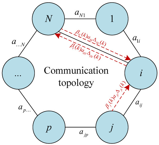
The communication of system (1) with network uncertainties is illustrated in Figure 1. Agent i can receive and transmit information from agents 1, j, and N. However, there may exist some additional communication channels owing to malicious topology attacks and so on. For example, agent i may receive additional information (i.e., $a_{ji}{\Delta }_{ji}\left(k\right)$ and $a_{Ni}{\Delta }_{Ni}\left(k\right)$) from agent j and agent N, whereas agent N can obtain additional information from agent i.

Figure 1. Framework of network uncertainties.

Remark 3.

The modeled uncertainty communication channel exhibits broad applicability, effectively capturing various complex faults within digital networks. For example, precision loss stemming from signal quantization during signal transmission, packet loss, communication noise associated with system states, and malicious topological attacks [25,26,27,28]. Furthermore, by introducing the independent Bernoulli random variables $\alpha \left(k\right)$ and ${\beta }_i\left(k\right)$, different types of uncertainties can be decoupled. This assumption ensures that the model can handle multiple uncertainties. Therefore, the established model has a broad generality.

Let $e_i\left(k\right)=x_i\left(k\right)-{\displaystyle \frac{1}{N}}{\displaystyle \sum _{j=1}^N}{x}_j\left(k\right)$ be the state of system error. Then, by using the Kronecker product, it follows from (4) that

$$u\left(k\right)=-\mu \left((\mathcal{L}+\Theta (k)\Pi (k\left)\right)\otimes K\right)x\left(k\right),$$

(6)

where $\Theta \left(k\right)=\mathrm{diag}\{{\beta }_1\left(k\right),{\beta }_2\left(k\right),\dots ,{\beta }_N\left(k\right)\}$ is a diagonal matrix, and the control input vector, state vector, error vector, and external disturbance are given by $u\left(k\right)={[u_1^T\left(k\right),u_2^T\left(k\right),\dots ,u_N^T\left(k\right)]}^T$, $x\left(k\right)={[x_1^T\left(k\right),x_2^T\left(k\right),\dots ,x_N^T\left(k\right)]}^T$, $w\left(k\right)=[w_1^{\mathrm{T}}\left(k\right),w_2^{\mathrm{T}}\left(k\right),\dots ,$$w_N^{\mathrm{T}}{\left(k\right)]}^{\mathrm{T}}$, $e\left(k\right)={[e_1^T\left(k\right),e_2^T\left(k\right),\dots ,e_N^T\left(k\right)]}^T=(M\otimes I_N)x\left(k\right)$, where $M=I_N-{\displaystyle \frac{1}{N}}{\mathbf{1}}_N{\mathbf{1}}_N^T$ such that $M\mathcal{L}=\mathcal{L}M=\mathcal{L}$. Therefore, the following error system can be obtained:

$$\begin{array}{c}e(k+1)=(I_N\otimes A\left(k\right)-\mu M(\mathcal{L}+\Theta \left(k\right)\Pi \left(k\right))\otimes BK)e\left(k\right)+(M\otimes C)w\left(k\right)\end{array}$$

(7)

and

$$\Pi \left(k\right)=\left[\begin{array}{ccc}{\displaystyle \sum _{j=1}^N}{a}_{1j}{\Delta }_{1j}\left(k\right)& \dots & -a_{1N}{\Delta }_{1N}\left(k\right)\\ ⋮& \ddots & ⋮\\ -a_{N1}{\Delta }_{N1}\left(k\right)& \dots & {\displaystyle \sum _{j=1}^N}{a}_{Nj}{\Delta }_{Nj}\left(k\right)\end{array}\right].$$

(8)

Remark 4.

Note that the network uncertainties modeled in (4) can be different between agent i and agent j, i.e., ${\Delta }_{ij}\left(k\right)\ne {\Delta }_{ji}\left(k\right)$, even if an undirected graph is considered. This results in $\Pi \left(k\right)$ not being a symmetric matrix, which poses some challenges in dealing with such uncertainties. Moreover, this indicates that external edges will not appear if there is originally no communication between any two agents. As illustrated in Figure 1, an undirected graph indicates that $a_{Ni}=a_{iN}$, but the uncertainties ${\Delta }_{Ni}\left(k\right)$ and ${\Delta }_{iN}\left(k\right)$ can be different, or clearly, one can check that ${\Delta }_{ji}\left(k\right)\equiv 0$.

2.4. Necessary Assumptions, Lemmas, and Definitions

Some assumptions, lemmas, and definitions are required to derive the main results.

Definition 1

([29]). System (1) is said to achieve mean-square quasi-consensus for any initial condition:

(1) 

if $w\left(k\right)\equiv 0$, there exist positive scales $M_0$ and ${\lambda }_0\in (0,1)$ such that $\mathbb{E}\left\{\right|e\left(k\right)\left|\right\}\le M_o{\lambda }_0^{k-k_0}$ for any $k>k_0$;

(2) 

if $w\left(k\right)\ne 0$, $e\left(k\right)$ exponentially converges into a bounded compact set $\mathcal{E}$ as $k\to +\infty$, where $\mathcal{E}:=\{e\in {\mathbb{R}}^{Nn}:\mathbb{E}\left\{\right|e\left|\right\}\le \vartheta \}$, and $\vartheta >0$ is called the error boundedness.

Assumption 1.

The communication topology of MAS (1) is represented by an undirected connected graph.

Assumption 2.

$w_i\left(k\right)$ in (1) is bounded, satisfying ${sup}_{k\in \mathbb{N}}\left|w_i\left(k\right)\right|\le w_{sup}<+\infty$.

Assumption 3.

There exists a function $\pi :\mathbb{N}\to \mathbb{R}$ such that $|{\Pi }^T\left(k\right)\Pi \left(k\right)|\le {\pi }^2\left(k\right)$.

Remark 5.

Under the above assumptions, $\Pi \left(k\right)$ characterizes the time-varying nature of the network topology, reflecting the dynamic changes in the network state. The function $\pi \left(k\right)$ represents the absolute upper bound of the uncertainty, ensuring that the system remains bounded under all circumstances.

Lemma 1

([30]). For any $r\in {\mathbb{R}}^q$, $\theta >0$, $v\in {\mathbb{R}}^l$, and $W\in {\mathbb{R}}^{q\times l}$, there always exists a positive-definite matrix $G\in {\mathbb{R}}^{l\times l}$ such that $2r^{T}Wv\le \theta r^{T}WG{W}^{T}r+{\theta }^{-1}{v}^T{G}^{-1}v$.

Lemma 2

([31]). Under Assumption 1, only one eigenvalue of $\mathcal{L}$ is zero, and the real part of the other eigenvalues of $N-1$ is positive. Then, there exists a unitary matrix $U\in {\mathbb{R}}^{N\times N}$, $U=[{\mathbf{1}}_N/\sqrt{N},U_1]$ such that $\Lambda =U^{-1}\mathcal{L}U=\left[\begin{array}{cc}0& 0\\ 0& J\end{array}\right]$, where $J=\mathit{diag}\{{\lambda }_2,{\lambda }_3,\dots ,{\lambda }_N\}$.

Lemma 3

([32]). Let $P\left(\gamma \right)>0$ be the unique solution to the following parametric algebraic Riccati equation

$$A_0^{\mathrm{T}}P\left(\gamma \right)A_0-A_0^{\mathrm{T}}P\left(\gamma \right)BK\left(\gamma \right)=(1-\gamma )P\left(\gamma \right),$$

(9)

where $\gamma \in (0,1)$ and $K\left(\gamma \right)={(B^{T}P\left(\gamma \right)B+I_n)}^{-1}{B}^{T}P\left(\gamma \right)A_0$. For the convenience of calculation, P and K are used to represent $P\left(\gamma \right)$ and $K\left(\gamma \right)$ below. Then,

$$\begin{array}{c}\hfill K^{\mathrm{T}}{B}^{\mathrm{T}}PBK\le {\displaystyle \frac{{\left({det}^2\left(A_0\right)-{(1-\gamma )}^n\right)}^2}{{(1-\gamma )}^{2n-1}}}P,\end{array}$$

(10)

$$\begin{array}{c}\hfill K^{\mathrm{T}}K\le K^{\mathrm{T}}(B^{\mathrm{T}}PB+I)K\le {\displaystyle \frac{{det}^2\left(A_0\right)-{(1-\gamma )}^n}{{(1-\gamma )}^{n-1}}}P.\end{array}$$

(11)

Based on Lemma 3, we can deduce the following lemma:

Lemma 4.

Suppose that $P>0$ is a unique solution to (9) and $K={(B^{\mathrm{T}}PB+I_n)}^{-1}{B}^{\mathrm{T}}P{A}_0$. If scales $\gamma \in (0,1)$ and $\mu >0$ exist such that

$$\begin{array}{c}\underset{i\in \{2,\dots N\}}{max}|\mu {\lambda }_i-1|\le \sqrt{{\displaystyle \frac{(g\left(\gamma \right)+\gamma -1){(1-\gamma )}^{n-1}}{{det}^2\left(A_0\right)-{(1-\gamma )}^n}}}:=\sigma \hfill \end{array},$$

(12)

where $g:{\mathbb{R}}^{+}\to (1-\gamma ,+\infty )$, then we obtain

$$\underset{i\in \{2,\dots N\}}{max}\left\{\rho \left(A_0-\mu {\lambda }_{i}BK\right)\right\}\le \sqrt{g\left(\gamma \right)}.$$

(13)

Proof. 

With the special form of K,

$$A_0^{\mathrm{T}}PBK=A_0^{\mathrm{T}}PB{(B^{\mathrm{T}}PB+I)}^{-1}(B^{\mathrm{T}}PB+I)K=K^{\mathrm{T}}(B^{\mathrm{T}}PB+I)K,$$

(14)

and from (9), we get

$$A_0^{\mathrm{T}}P{A}_0=A_0^{\mathrm{T}}P\left(\gamma \right)BK\left(\gamma \right)+(1-\gamma )P\left(\gamma \right).$$

(15)

   □

For any complex number $s=a+\mathrm{j}b$, from (14) and (15), we obtain

$$\begin{array}{cc}\hfill & {(A_0-s\mu BK)}^{\ast }P(A_0-s\mu BK)\hfill \\ \hfill & ={(A_0-a\mu BK)}^{\mathrm{T}}P(A_0-a\mu BK)+b^2{\mu }^2{K}^{\mathrm{T}}{B}^{\mathrm{T}}PBK\hfill \\ \hfill & =(1-2a\mu +(a^2+b^2){\mu }^2)K^{\mathrm{T}}{B}^{\mathrm{T}}PBK+(1-2a\mu )K^{\mathrm{T}}K-(\gamma -1)P\hfill \\ \hfill & \le ((1-2a\mu )+(a^2+b^2){\mu }^2)K^{\mathrm{T}}(B^{\mathrm{T}}PB+I)K-(\gamma -1)P\hfill \\ \hfill & =((\mu a-1)+\mathrm{j}\mu b))\left(((\mu a-1)-\mathrm{j}\mu b)\right)K^{\mathrm{T}}(B^{\mathrm{T}}PB+I)K-(\gamma -1)P\hfill \\ \hfill & ={\left|s\mu -1\right|}^2{K}^{\mathrm{T}}(B^{\mathrm{T}}PB+I)K-(\gamma -1)P\hfill \\ \hfill & \le {\displaystyle \frac{({det}^2\left(A_0\right)-{(1-\gamma )}^n){\left|s\mu -1\right|}^2}{{(1-\gamma )}^{n-1}}}P-(\gamma -1)P.\hfill \end{array}$$

(16)

where $a^2+b^2\ge 0$ is noted in the first inequality, and (11) is used to obtain the last inequality.

Note that if the condition

$$\left|s\mu -1\right|\le \sqrt{{\displaystyle \frac{(g\left(\gamma \right)+\gamma -1){(1-\gamma )}^{n-1}}{{det}^2\left(A_0\right)-{(1-\gamma )}^n}}}=\sigma$$

(17)

holds, then we get

$${(A_0-s\mu BK)}^{\ast }P(A_0-s\mu BK)\le g\left(\gamma \right)P.$$

(18)

Note that, the complex number s can represent any eigenvalue of the Laplacian matrix $\mathcal{L}$; then, ${max}_{i\in \{2,\dots N\}}\left|\mu {\lambda }_i-1\right|\le \sigma$. As a result, we further obtain

$${(A_0-\mu {\lambda }_{i}BK)}^{\ast }P(A_0-\mu {\lambda }_{i}BK)\le g\left(\gamma \right)P.$$

(19)

Let h be any non-zero vector. Then, conclusion (12) can be derived as follows

$$\begin{array}{cc}\hfill & h^{\ast }{(A_0-\mu {\lambda }_{i}BK)}^{\ast }P(A_0-\mu {\lambda }_{i}BK)h\hfill \\ \hfill & =h^{\ast }\overline{\lambda }(A_0-\mu {\lambda }_{i}BK)P\lambda (A_0-\mu {\lambda }_{i}BK)h\hfill \\ \hfill & ={\rho }^2(A_0-\mu {\lambda }_{i}BK)h^{\ast }Ph\le g\left(\gamma \right)h^{\ast }Ph.\hfill \end{array}$$

(20)

Remark 6.

Because of the characteristics of the parametric algebraic Riccati equation, some simple conditions can be obtained, and the scalar parameter μ can be independent of ${\lambda }_2$, which is different from the conclusions of the existing literature [33]. In addition, compared with the literature [18,19,33], control matrix B in (1) does not need to satisfy the full-rank condition, which makes it more universal and applicable.

3. Main Results

Theorem 1.

Suppose that Assumptions 1–3 are satisfied. Then, MASs (1) can reach the mean-square quasi-consensus under protocol (4) with $K={(B^{\mathrm{T}}PB+I_n)}^{-1}{B}^{\mathrm{T}}P{A}_0$ if the following conditions hold:

$$\left[\begin{array}{cc}-Q& S^{T}P\\ ★& -P\end{array}\right]<0,$$

(21)

$$\left[\begin{array}{cc}{\displaystyle \frac{{\epsilon }_1+2}{{\epsilon }_1}}{K}^T{B}^{T}PBK-{\mu }_{1}P& \sqrt{{\epsilon }_2}{K}^T{B}^{T}PSQ\\ ★& -Q\end{array}\right]<0,$$

(22)

$$\left[\begin{array}{cc}(1+{\epsilon }_1^{-1}+{\epsilon }_1)C^{\mathrm{T}}PC-{\mu }_{2}P& \sqrt{{\epsilon }_2}{C}^{\mathrm{T}}PS\\ ★& -Q\end{array}\right]<0,$$

(23)

$$\prod _{l=s}^{k-1}\overline{g}(\gamma ,l)\le {\overline{g}}_0{\lambda }^{k-s},\forall k>s\ge 0,$$

(24)

where ${\epsilon }_1,{\epsilon }_2,{\mu }_1,{\mu }_2>0$, ${\overline{g}}_0\ge 1$, and $\lambda \in (0,1)$ are some scales, and $\overline{g}:(0,1)\times \mathbb{N}\to {\mathbb{R}}^{+}$, where

$$\begin{array}{c}\hfill \overline{g}(\gamma ,k)=\kappa \overline{\epsilon }+(1+3{\epsilon }_1)g\left(\gamma \right)+{\mu }_1{\mu }^2{\beta }_{max}^2{\pi }^2\left(k\right),\end{array}$$

(25)

where $\kappa ={\alpha }_0^2{H}_0{\lambda }_{max}\left(R^{T}R\right)/{\lambda }_{min}\left(P\right)$, $\overline{\epsilon }=1+{\epsilon }_1^{-1}+2{\epsilon }_2^{-1}$.

Moreover, the upper error boundedness can be estimated as

$$\vartheta =\sqrt{{\displaystyle \frac{{\mu }_2{\overline{g}}_0{\lambda }_{max}\left(P\right)}{{\lambda }_{min}\left(P\right)(1-\lambda )}}}{w}_{sup}.$$

(26)

Proof. 

In this proof, two cases, $w\left(k\right)\ne 0$ and $w\left(k\right)\equiv 0$ are considered. When $w\left(k\right)\ne 0$, let $z\left(k\right)=(U^T\otimes I_n)e\left(k\right)$. It can be seen that

$$(1_N^{\mathrm{T}}/N\otimes I_n)e\left(k\right)=(1_N^{\mathrm{T}}M/N\otimes I_n)x\left(k\right)\equiv 0.$$

(27)

   □

Therefore, $z_1\left(k\right)\equiv 0$ can be obtained, and from Equation (7), we obtain

$$\begin{array}{cc}\overline{z}(k+1)\hfill & =({\overline{A}}_0+\overline{B}\left(k\right)-\overline{C}\left(k\right))\overline{z}\left(k\right)+(U_1^{T}M\otimes C)w\left(k\right),\hfill \end{array}$$

(28)

where

$$\begin{array}{c}\overline{z}\left(k\right)={[z_2^{\mathrm{T}}\left(k\right),z_3^{\mathrm{T}}\left(k\right),\dots ,z_N^{\mathrm{T}}\left(k\right)]}^{\mathrm{T}},{\overline{A}}_0=I_{N-1}\otimes A_0-\mu J\otimes BK,\hfill \\ \overline{B}\left(k\right)=I_{N-1}\otimes \alpha \left(k\right)SH\left(k\right)R,\overline{C}\left(k\right)=\mu U_1^T\Theta \left(k\right)\Pi \left(k\right)U_1\otimes BK.\end{array}$$

(29)

Consider the candidate Lyapunov function

$$V\left(z\left(k\right)\right)=z^T\left(k\right)(I_N\otimes P)z\left(k\right).$$

(30)

From this we can obtain

$$\begin{array}{cc}V\left(z\right(k+1\left)\right)\hfill & ={\overline{z}}^{\mathrm{T}}\left(k\right){\overline{A}}_0^{\mathrm{T}}(I_{N-1}\otimes P){\overline{A}}_0\overline{z}\left(k\right)+{\overline{z}}^{\mathrm{T}}\left(k\right){\overline{B}}^{\mathrm{T}}\left(k\right)(I_{N-1}\otimes P)\overline{B}\left(k\right)\overline{z}\left(k\right)\hfill \\ \hfill & +{\overline{z}}^{\mathrm{T}}\left(k\right){\overline{C}}^{\mathrm{T}}\left(k\right)(I_{N-1}\otimes P)\overline{C}\left(k\right)\overline{z}\left(k\right)+w^{\mathrm{T}}\left(k\right)(M\otimes C^{\mathrm{T}}PC)w\left(k\right)\hfill \\ \hfill & +2{\overline{z}}^T\left(k\right){\overline{A}}_0^{\mathrm{T}}(I_{N-1}\otimes P)\overline{B}\left(k\right)\overline{z}\left(k\right)-2{\overline{z}}^{\mathrm{T}}\left(k\right){\overline{A}}_0^{\mathrm{T}}(I_{N-1}\otimes P)\overline{C}\left(k\right)\overline{z}\left(k\right)\hfill \\ \hfill & +2{\overline{z}}^{\mathrm{T}}\left(k\right){\overline{A}}_0^{\mathrm{T}}\left(U_1^{\mathrm{T}}MPC\right)w\left(k\right)-2{\overline{z}}^{\mathrm{T}}\left(k\right){\overline{B}}^{\mathrm{T}}\left(k\right)(I_{N-1}\otimes P)\overline{C}\left(k\right)\overline{z}\left(k\right)\hfill \\ \hfill & +2{\overline{z}}^{\mathrm{T}}\left(k\right){\overline{B}}^{\mathrm{T}}\left(k\right)(U_1^{\mathrm{T}}M\otimes PC)w\left(k\right)-2{\overline{z}}^{\mathrm{T}}\left(k\right){\overline{C}}^T\left(k\right)(U_1^{\mathrm{T}}M\otimes PC)w\left(k\right).\hfill \end{array}$$

(31)

From Lemma 2, we can easily obtain $U_1{U}_1^{\mathrm{T}}=M$, $MM=M$, and from Lemma 1, we obtain

$$\begin{array}{cc}\hfill & 2{\overline{z}}^{\mathrm{T}}\left(k\right){\overline{A}}_0^{\mathrm{T}}(I_{N-1}\otimes P)\overline{B}\left(k\right)\overline{z}\left(k\right)\hfill \\ \hfill & \le {\epsilon }_1{\overline{z}}^{\mathrm{T}}\left(k\right){\overline{A}}_0^{\mathrm{T}}(I_{N-1}\otimes P){\overline{A}}_0\overline{z}\left(k\right)+{\epsilon }_1^{-1}{\overline{z}}^{\mathrm{T}}\left(k\right){\overline{B}}^{\mathrm{T}}\left(k\right)(I_{N-1}\otimes P)\overline{B}\left(k\right)\overline{z}\left(k\right),\hfill \end{array}$$

(32)

and

$$\begin{array}{cc}\hfill & -2{\overline{z}}^{\mathrm{T}}\left(k\right){\overline{A}}_0^{\mathrm{T}}(I_{N-1}\otimes P)\overline{C}\left(k\right)\overline{z}\left(k\right)\hfill \\ \hfill & \le {\epsilon }_1{\overline{z}}^{\mathrm{T}}\left(k\right){\overline{A}}_0^{\mathrm{T}}(I_{N-1}\otimes P){\overline{A}}_0\overline{z}\left(k\right)+{\epsilon }_1^{-1}{\overline{z}}^{\mathrm{T}}\left(k\right){\overline{C}}^{\mathrm{T}}\left(k\right)(I_{N-1}\otimes P)\overline{C}\left(k\right)\overline{z}\left(k\right),\hfill \end{array}$$

(33)

and

$$\begin{array}{cc}\hfill & 2{\overline{z}}^{\mathrm{T}}\left(k\right){\overline{A}}_0^{\mathrm{T}}(U_1^{\mathrm{T}}M\otimes PC)w\left(k\right)\hfill \\ \hfill & \le {\epsilon }_1{\overline{z}}^{\mathrm{T}}\left(k\right){\overline{A}}_0^{\mathrm{T}}(I_{N-1}\otimes P){\overline{A}}_0\overline{z}\left(k\right)+{\epsilon }_1^{-1}{w}^{\mathrm{T}}\left(k\right)(M\otimes C^{\mathrm{T}}PC)w\left(k\right).\hfill \end{array}$$

(34)

Furthermore, with Lemma 4 and (21), substituting (32)–(34) into (31) yields

$$\begin{array}{cc}V\left(z\right(k+1\left)\right)\hfill & \le \left((1+3{\epsilon }_1)g\left(\gamma \right)+(1+{\epsilon }_1^{-1})\kappa \right)V\left(z\left(k\right)\right)\hfill \\ \hfill & +(1+{\epsilon }_1^{-1}){\overline{z}}^{\mathrm{T}}\left(k\right){\overline{C}}^{\mathrm{T}}\left(k\right)(I_{N-1}\otimes P)\overline{C}\left(k\right)\overline{z}\left(k\right)\hfill \\ \hfill & +(1+{\epsilon }_1^{-1})w^{\mathrm{T}}\left(k\right)(M\otimes C^{\mathrm{T}}PC)w\left(k\right)\hfill \\ \hfill & +2\alpha \left(k\right){\overline{z}}^T\left(k\right)(U_1^{\mathrm{T}}M\otimes R^{\mathrm{T}}{H}^{\mathrm{T}}\left(k\right)S^{\mathrm{T}}PC)w\left(k\right)\hfill \\ \hfill & -2\mu {\overline{z}}^{\mathrm{T}}\left(k\right)(U_1^{\mathrm{T}}\Theta \left(k\right){\Pi }^{\mathrm{T}}\left(k\right)M\otimes K^{\mathrm{T}}{B}^{\mathrm{T}}PC)w\left(k\right)\hfill \\ \hfill & -2\mu \alpha \left(k\right){\overline{z}}^{\mathrm{T}}\left(k\right)(U_1^{\mathrm{T}}\Theta \left(k\right)\Pi \left(k\right)U_1{R}^{\mathrm{T}}{H}^{\mathrm{T}}\left(k\right)S^{\mathrm{T}}PBK)\overline{z}\left(k\right),\hfill \end{array}$$

(35)

where we obtain noted that $M<I$, $U_1^T{U}_1=I_{N-1}$. Since

$$\begin{array}{cc}\hfill U_1^{\mathrm{T}}{\Pi }^{\mathrm{T}}\left(k\right)U_1{U}_1^{\mathrm{T}}\Pi \left(k\right)U_1& =U_1^{\mathrm{T}}{\Pi }^{\mathrm{T}}\left(k\right)M\Pi \left(k\right)U_1\le U_1^{\mathrm{T}}{\Pi }^{\mathrm{T}}\left(k\right)\Pi \left(k\right)U_1\hfill \\ \hfill & \le |{\Pi }^{\mathrm{T}}\left(k\right)\Pi \left(k\right)|I_{N-1},\hfill \end{array}$$

(36)

from which, using Lemma 1, it follows from (2) and (5) that

$$\begin{array}{cc}\hfill & \mathbb{E}\{-2\mu {\overline{z}}^{\mathrm{T}}\left(k\right)(U_1^{\mathrm{T}}\Theta \left(k\right)\Pi \left(k\right)U_1\otimes R^{\mathrm{T}}{H}^{\mathrm{T}}\left(k\right)S^{\mathrm{T}}PBK)\overline{z}\left(k\right)\}\hfill \\ \hfill & \le {\epsilon }_2^{-1}{\alpha }_0^2\mathbb{E}\left\{{\overline{z}}^{\mathrm{T}}\left(k\right)(I_{N-1}\otimes R^{\mathrm{T}}{H}^{\mathrm{T}}\left(k\right)QH\left(k\right)R)\overline{z}\left(k\right)\right\}\hfill \\ \hfill & +{\epsilon }_2{\mu }^2{\beta }_{max}^2|{\Pi }^{\mathrm{T}}\left(k\right)\Pi \left(k\right)|\mathbb{E}\left\{{\overline{z}}^{\mathrm{T}}\left(k\right)(I_{N-1}\otimes K^{\mathrm{T}}{B}^{\mathrm{T}}PS{Q}^{-1}{S}^{\mathrm{T}}PBK)\overline{z}\left(k\right)\right\},\hfill \end{array}$$

(37)

and

$$\begin{array}{cc}\hfill & \mathbb{E}\left\{2\alpha \left(k\right){\overline{z}}^{\mathrm{T}}\left(k\right)(U_1^{\mathrm{T}}M\otimes R^{\mathrm{T}}{H}^{\mathrm{T}}\left(k\right)S^{\mathrm{T}}PC)w\left(k\right)\right\}\hfill \\ \hfill & \le {\epsilon }_2^{-1}{\alpha }_0^2\mathbb{E}\left\{{\overline{z}}^{\mathrm{T}}\left(k\right)(I_{N-1}\otimes R^{\mathrm{T}}{H}^{\mathrm{T}}\left(k\right)QH\left(k\right)R)\overline{z}\left(k\right)\right\}\hfill \\ \hfill & +{\epsilon }_2{w}^{\mathrm{T}}\left(k\right)(I_{N-1}\otimes C^{\mathrm{T}}PS{Q}^{-1}{S}^{\mathrm{T}}PC)w\left(k\right),\hfill \end{array}$$

(38)

and

$$\begin{array}{cc}\hfill & \mathbb{E}\{-2\mu {\overline{z}}^{\mathrm{T}}\left(k\right)(U_1^{\mathrm{T}}\Theta \left(k\right){\Pi }^{\mathrm{T}}\left(k\right)M\otimes K^{\mathrm{T}}{B}^{\mathrm{T}}PC)w\left(k\right)\}\hfill \\ \hfill & \le {\epsilon }_1^{-1}{\mu }^2{\beta }_{max}^2|{\Pi }^{\mathrm{T}}\left(k\right)\Pi \left(k\right)|\mathbb{E}\left\{{\overline{z}}^{\mathrm{T}}\left(k\right)(I_{N-1}\otimes K^{\mathrm{T}}{B}^{\mathrm{T}}PBK)\overline{z}\left(k\right)\right\}\hfill \\ \hfill & +{\epsilon }_1{w}^{\mathrm{T}}\left(k\right)(I_{N-1}\otimes C^{\mathrm{T}}PC)w\left(k\right).\hfill \end{array}$$

(39)

Substituting (37)–(39) into (35) and taking the expectation operation on both sides, we obtain

$$\begin{array}{cc}\hfill \mathbb{E}\left\{V\right(z(k+1)\left)\right\}& \le \left(\kappa \overline{\epsilon }+(1+3{\epsilon }_1)g\left(\gamma \right)\right)\mathbb{E}\left\{V\left(z\left(k\right)\right)\right\}\hfill \\ \hfill & +{\mu }^2{\beta }_{max}^2\left|{\Pi }^{\mathrm{T}}\left(k\right)\Pi \left(k\right)\right|\mathbb{E}\{(1+2{\epsilon }_1^{-1}){\overline{z}}^{\mathrm{T}}\left(k\right)(I_{N-1}\otimes K^{\mathrm{T}}{B}^{\mathrm{T}}PBK)\overline{z}\left(k\right)\hfill \\ \hfill & +{\epsilon }_2{\overline{z}}^{\mathrm{T}}\left(k\right)(I_{N-1}\otimes K^{\mathrm{T}}{B}^{\mathrm{T}}PS{Q}^{-1}{S}^{\mathrm{T}}PBK)\overline{z}\left(k\right)\}\hfill \\ \hfill & +{\epsilon }_2{w}^{\mathrm{T}}\left(k\right)(I_{N-1}\otimes C^{\mathrm{T}}PS{Q}^{-1}{S}^{\mathrm{T}}PC)w\left(k\right)\hfill \\ \hfill & +(1+{\epsilon }_1^{-1}+{\epsilon }_1)w^{\mathrm{T}}\left(k\right)(I_{N-1}\otimes C^{\mathrm{T}}PC)w\left(k\right),\hfill \end{array}$$

(40)

from which by using (22) and (23), we get

$$\begin{array}{c}\mathbb{E}\left\{V\left(z(k+1)\right)\right\}\le \overline{g}(\gamma ,k)\mathbb{E}\left\{V\left(z\left(k\right)\right)\right\}+{\mu }_2{w}^{\mathrm{T}}\left(k\right)(I_N\otimes P)w\left(k\right).\end{array}$$

(41)

Clearly, by iterating and using (24), we can conclude that

$$\begin{array}{cc}\hfill \mathbb{E}\left\{V\right(z\left(k\right)\left)\right\}& \le \prod _{l=0}^{k-1}\overline{g}(\gamma ,l)\mathbb{E}\left\{V\left(z\left(0\right)\right)\right\}+{\mu }_2{w}_{sup}^2{\lambda }_{max}\left(P\right)\sum _{l=0}^{k-1}\prod _{j=l+1}^{k-1}\overline{g}(\gamma ,j)\hfill \\ \hfill & \le {\overline{g}}_0{\overline{\lambda }}^k\mathbb{E}\left\{V\left(z\left(0\right)\right)\right\}+{\displaystyle \frac{{\mu }_2{\overline{g}}_0{\lambda }_{max}\left(P\right)}{1-\overline{\lambda }}}{w}_{sup}^2,\hfill \end{array}$$

(42)

which indicates that

$$\underset{k\to +\infty }{limsup}\mathbb{E}\left\{\right|z\left(k\right)\left|\right\}\le \sqrt{{\displaystyle \frac{{\mu }_2{\overline{g}}_0{\lambda }_{max}\left(P\right)}{{\lambda }_{min}\left(P\right)(1-\overline{\lambda })}}}{w}_{sup}.$$

(43)

And with ${\left|z\left(k\right)\right|}^2=\left|e^{\mathrm{T}}\left(k\right)(U{U}^{\mathrm{T}}\otimes I_n)e\left(k\right)\right|=|e\left(k\right){|}^2$, we can further obtain

$$\underset{k\to +\infty }{limsup}\mathbb{E}\left\{\right|e\left(k\right)\left|\right\}\le \sqrt{{\displaystyle \frac{{\mu }_2{\overline{g}}_0{\lambda }_{max}\left(P\right)}{{\lambda }_{min}\left(P\right)(1-\overline{\lambda })}}}{w}_{sup}:=\vartheta .$$

(44)

On the other hand, when $w\left(k\right)\equiv 0$, we can also derive from (31) that

$$\begin{array}{cc}\hfill V\left(z\right(k+1\left)\right)& ={\overline{z}}^T\left(k\right){\overline{A}}_0^T(I_{N-1}\otimes P){\overline{A}}_0\overline{z}\left(k\right)+{\overline{z}}^T\left(k\right){\overline{B}}^T\left(k\right)(I_{N-1}\otimes P)\overline{B}\left(k\right)\overline{z}\left(k\right)\hfill \\ \hfill & +{\overline{z}}^T\left(k\right){\overline{C}}^T\left(k\right)(I_{N-1}\otimes P)\overline{C}\left(k\right)\overline{z}\left(k\right)+2{\overline{z}}^T\left(k\right){\overline{A}}_0^T(I_{N-1}\otimes P)\overline{B}\left(k\right)\overline{z}\left(k\right)\hfill \\ \hfill & -2{\overline{z}}^T\left(k\right){\overline{A}}_0^T(I_{N-1}\otimes P)\overline{C}\left(k\right)\overline{z}\left(k\right)-2{\overline{z}}^T\left(k\right){\overline{B}}^T\left(k\right)(I_{N-1}\otimes P)\overline{C}\left(k\right)\overline{z}\left(k\right).\hfill \end{array}$$

(45)

Applying Equations (32), (33), (37), and (21) we obtain

$$\begin{array}{c}\mathbb{E}\left\{V\left(z(k+1)\right)\right\}\le \widehat{g}(\gamma ,k)\mathbb{E}\left\{V\left(z\left(k\right)\right)\right\}\le \overline{g}(\gamma ,k)\mathbb{E}\left\{V\left(z\left(k\right)\right)\right\},\hfill \end{array}$$

(46)

where $\widehat{g}(\gamma ,k)=\kappa \tilde{\epsilon }+(1+2{\epsilon }_1)g\left(\gamma \right)+{\overline{\mu }}_1{\mu }^2{\beta }_{max}^2{\pi }^2\left(k\right)$, $\tilde{\epsilon }=1+{\epsilon }_1^{-1}+{\epsilon }_2^{-1}$ and the scalar parameter ${\overline{\mu }}_1>0$ satisfies

$$\left[\begin{array}{cc}\left(1+{\epsilon }_1^{-1}\right)K^{\mathrm{T}}{B}^{\mathrm{T}}PBK-{\overline{\mu }}_{1}P& \sqrt{{\epsilon }_2}{K}^{\mathrm{T}}{B}^{\mathrm{T}}PSQ\\ ★& -Q\end{array}\right]<0.$$

(47)

Hence, we get

$$\begin{array}{c}\mathbb{E}\left\{V\left(z\left(k\right)\right)\right\}\le {\displaystyle \prod _{l=0}^{k-1}}\overline{g}(\gamma ,l)\mathbb{E}\left\{V\left(z\left(0\right)\right)\right\}\le {\overline{g}}_0{\overline{\lambda }}^k\mathbb{E}\left\{V\left(z\left(0\right)\right)\right\},\end{array}$$

(48)

which indicates that $\left|z\right(k\left)\right|$ can exponentially converge to zero when $w\left(k\right)\equiv 0$.

Combining with the above two cases, we can conclude that $\left|e\right(k\left)\right|$ can exponentially converge into a bounded set $\mathcal{E}$ with the converge rate $\lambda$, and the error boundedness can be estimated as $\vartheta$ as $k\to +\infty$, where $\mathcal{E}=\{e\in {\mathbb{R}}^{Nn}:|e|\le \vartheta \}$. Therefore, according to Definition 1, the disturbed discrete-time linear MASs (1) can achieve mean-square quasi-consensus under control protocol (4), and its error upper boundedness can be estimated as $\vartheta$. This completes this proof.

Remark 7.

Compared to the assumptions in [18,19], network uncertainties here are fully used, which leads to the time-shift in the Lyapunov function being non-decreasing when $w\left(k\right)\equiv 0$, i.e.,

$$\begin{array}{cc}\hfill \Delta V\left(z\right(k\left)\right)& =V\left(z(k+1)\right)-V\left(z\left(k\right)\right)=(\widehat{g}(\gamma ,k)-1)V\left(z\left(k\right)\right)\hfill \\ \hfill & \Rightarrow \left\{\begin{array}{c}\Delta V\left(z\left(k\right)\right)\ge 0\mathrm{when}\widehat{g}(\gamma ,k)\ge 1,\\ \Delta V\left(z\left(k\right)\right)<0\mathrm{when}\widehat{g}(\gamma ,k)<1,\end{array}\right.\hfill \end{array}$$

(49)

whereas system (1) can reach a mean-square quasi-consensus with an exponential convergence rate. In addition, conditions in Theorem 4.2 in [18] directly use the Mahler measure of A, which leads to much conservatism when systems are unstable, i.e., eigenvalues outside the unit circle. Therefore, more general results were obtained in this study.

Remark 8.

For Equation (25), appropriate parameters must be selected to satisfy condition (24). Because Equation (25) has a time-varying characteristic, it is difficult to directly obtain the supremum of $\pi \left(k\right)$ in Assumption 3. However, if $k>k_0$ holds for all $\overline{g}\left(\gamma ,k\right)<1$, the supremum of $\pi \left(k\right)$ can be easily determined as $\underset{k\in \mathbb{N}}{sup}\left\{\pi \left(k\right)\right\}<\sqrt{{\displaystyle \frac{\kappa \overline{\epsilon }+(1+3{\epsilon }_1)g\left(\gamma \right)}{{\mu }_1{\mu }^2{\beta }_{max}^2}}}$.

In addition, if ${\Delta }_{ij}\left(k\right)\equiv \overline{\Delta }\in \mathbb{R}$, the following easily verifiable condition can be obtained.

Corollary 1.

Suppose that Assumptions 1–3 are satisfied, ${\beta }_i\left(k\right)\equiv 1$, and ${\Delta }_{ij}\left(k\right)\equiv \overline{\Delta }$. Then, MASs (1) can reach the mean-square quasi-consensus under protocol (4) with $K={(B^{\mathrm{T}}PB+I_n)}^{-1}{B}^{\mathrm{T}}P{A}_0$ if (21) and the following conditions hold

$$\left[\begin{array}{cc}(1+{\epsilon }_1^{-1})C^{T}PC-{\widehat{\mu }}_{2}P& \sqrt{{\epsilon }_2}{C}^{T}PS\\ ★& -Q\end{array}\right]<0,$$

(50)

$$\tilde{g}\left(\gamma \right)<1,$$

(51)

where ${\epsilon }_1,{\epsilon }_2,{\widehat{\mu }}_2>0$ are scalar parameters, and $\tilde{g}\left(\gamma \right)=\kappa \tilde{\epsilon }+(1+2{\epsilon }_1)g\left(\gamma \right)$.

Moreover, the upper error boundedness can be estimated as

$$\vartheta =\sqrt{{\displaystyle \frac{{\widehat{\mu }}_2{\lambda }_{max}\left(P\right)}{{\lambda }_{min}\left(P\right)(1-\tilde{g}\left(\gamma \right))}}}{w}_{sup}.$$

(52)

Proof. 

Because ${\beta }_i\left(k\right)\equiv 1$ and ${\Delta }_{ij}\left(k\right)\equiv \overline{\Delta }$, the error system (7) can be rewritten as

$$\begin{array}{cc}\hfill e(k+1)& =\left(I_N\otimes A\left(k\right)-\mu (1+\overline{\Delta })(\mathcal{L}\otimes BK\right)e\left(k\right)+(M\otimes C)w\left(k\right).\hfill \end{array}$$

(53)

   □

Similarly, we obtain $\overline{z}(k+1)=({\widehat{A}}_0+\overline{B}\left(k\right))\overline{z}\left(k\right)+(U_1^{\mathrm{T}}M\otimes C)w\left(k\right)$, where ${\widehat{A}}_0=I_{N-1}\otimes A_0-\overline{\mu }J\otimes BK$ and $\tilde{\mu }=\mu (1+\overline{\Delta })$. Choosing the candidate Lyapunov function (30), we get

$$\mathbb{E}\left\{V\left(z(k+1)\right)\right\}\le \tilde{g}\left(\gamma \right)\mathbb{E}\left\{V\left(z\left(k\right)\right)\right\}+{\widehat{\mu }}_2{w}^T\left(k\right)(I_N\otimes P)w\left(k\right).$$

(54)

The remainder is similar to that of Theorem 1, and the details are omitted here. The proof is completed.

Remark 9.

To explicitly clarify the parameter selection process and ensure the reproducibility of our work, Algorithm 1 is provided to determine the feasible range of γ for a given control gain scale μ. Additionally, while $g\left(\gamma \right)$ can be arbitrarily chosen in a certain sense, setting $g\left(\gamma \right)+\gamma -1=l\gamma$ with $l>0$ simplifies the computational complexity in (12).

Algorithm 1 The feasible range of $\gamma$ when $\mu$ is given

Input: k, $\mu$, ${\alpha }_0$, ${\beta }_{max}$, $\pi \left(k\right)$, $g\left(\gamma \right)$, n, $A_0$, B, C, S, R, $H\left(k\right)$, $\mathcal{L}$ {The number of iterations k must       be sufficiently large} Output: the feasible range of $\gamma \in [{\gamma }_{min},{\gamma }_{max}]$   1: ${\lambda }_2,{\lambda }_3,\dots ,{\lambda }_N\leftarrow$ Compute the $N-1$ non-zero eigenvalues of matrix $\mathcal{L}$   2: $\overline{\sigma }\leftarrow {max}_{i\in \{2,\dots N\}}|\mu {\lambda }_i-1|$   3: for  $\gamma =0:1/k:1$  do   4:    if $\overline{\sigma }\le \sigma$ in (12) then   5:      $K,P\leftarrow$ solve the parametric algebra Riccati Equation (9)   6:      ${\epsilon }_1,{\epsilon }_2,{\mu }_1,{\mu }_2,Q\leftarrow$ solve the linear matrix inequalities (21)–(23)   7:      $H_0\leftarrow$ solve $H^{\mathrm{T}}\left(k\right)QH\left(k\right)\le H_0{I}_n$   8:      $\kappa \leftarrow$${\alpha }_0^2{H}_0{\lambda }_{max}\left(R^{T}R\right)/{\lambda }_{min}\left(P\right)$, and $\overline{\epsilon }\leftarrow$$1+1/{\epsilon }_1+2/{\epsilon }_2$   9:      $\overline{g}(\gamma ,k)\leftarrow \kappa \overline{\epsilon }+(1+3{\epsilon }_1)g\left(\gamma \right)+{\mu }_1{\mu }^2{\beta }_{max}^2{\pi }^2\left(k\right)$ 10:      if $\overline{g}(\gamma ,k)\in (0,1)$ then 11:         ${\gamma }_{min}\leftarrow \gamma$  12:      end if $\overline{g}(\gamma ,k)>1$ then 13:         ${\gamma }_{max}\leftarrow \gamma$, and force to break from the while loop 14:      end if 15:    else 16:      continue 17:    end if 18: end for

4. Numerical Examples

This section verifies the effectiveness of the proposed method through numerical simulation. Consider a multi-agent system (1) with four agents, where

$$A_0=\left[\begin{array}{cc}0& 1\\ -1& 1\end{array}\right],B=\left[\begin{array}{c}0\hfill \\ 1\hfill \end{array}\right],C=\left[\begin{array}{cc}0.052& 0.01\\ 0.021& -0.028\end{array}\right],$$

and consider the communication topology, which is described as follows:

$$\mathcal{L}=\left[\begin{array}{cccc}3.33& -1.665& 0& -1.665\\ -1.665& 3.33& -1.665& 0\\ 0& -1.665& 3.33& -1.665\\ -1.665& 0& -1.665& 3.33\end{array}\right].$$

With parameters $\gamma =0.6,\mu =0.2$, and $g\left(\gamma \right)=1-0.5\gamma$, according to the parametric algebra Riccati Equation (9), we can obtain

$$K=\left[\begin{array}{cc}0.168& -0.12\end{array}\right]\mathrm{and}P=\left[\begin{array}{cc}2.1& -1.5\\ -1.5& 5.25\end{array}\right].$$

It has been verified that the value of $\gamma$ satisfies

$$\begin{array}{c}{\displaystyle \underset{i\in \{2,\dots N\}}{max}}|\mu {\lambda }_i-1|=0.334\le \sqrt{{\displaystyle \frac{(g\left(\gamma \right)+\gamma -1){(1-\gamma )}^{n-1}}{{det}^2\left(A_0\right)-{(1-\gamma )}^n}}}=0.378.\hfill \end{array}$$

For uncertainty, select parameters ${\alpha }_0=0.1$, ${\beta }_{max}=0.1$, and

$$S=\left[\begin{array}{cc}0.1& 0\\ 0& 0.1\end{array}\right],R=\left[\begin{array}{cc}0.2& 0\\ 0& 0.2\end{array}\right],H\left(k\right)=\left[\begin{array}{cc}0.58& 0.76\\ 0.33& 0.42\end{array}\right]\times sin\left(k\right),$$

$$\Pi \left(k\right)=\left[\begin{array}{cccc}0.225& 0.18& 0.195& 0.63\\ 0.675& 0.48& 0.87& 1.005\\ 0.225& 1.005& 0.87& 0.615\\ 0.48& 0.915& 0.72& 0.885\end{array}\right]\times sin\left({\displaystyle \frac{2\pi }{5}}k\right).$$

In addition, by solving the linear matrix inequalities (21)–(23), we obtain ${\epsilon }_1=0.1$, ${\epsilon }_2=1$, ${\mu }_1=1.5$, ${\mu }_2=0.05$, and

$$Q=\left[\begin{array}{cc}2.3247& 0.0196\\ 0.0196& 2.2615\end{array}\right].$$

Choose initial state values

$$x_1^{\mathrm{T}}\left(0\right)=[0.5,2],x_2^{\mathrm{T}}\left(0\right)=[-0.5,-1],x_3^{\mathrm{T}}\left(0\right)=[-1.5,-2],x_4^{\mathrm{T}}\left(0\right)=[2.5,-1.5],$$

and select

$$\begin{array}{cc}\hfill & w_1^{\mathrm{T}}\left(k\right)=[0.4cos\left(Tk\right),0.45sin\left(Tk\right)],w_2^{\mathrm{T}}\left(k\right)=[0.5sin\left(Tk\right),0.45cos\left(Tk\right)],\hfill \\ \hfill & w_3^{\mathrm{T}}\left(k\right)=[0.5sin\left(Tk\right),0.43sin\left(Tk\right)],w_4^{\mathrm{T}}\left(k\right)=[0.5cos\left(Tk\right),0.43cos\left(Tk\right)],\hfill \end{array}$$

where $T=15$, and $\lambda =0.919$ and ${\overline{g}}_0=1.01$ are selected such that Equation (25) satisfies condition (24). Therefore, based on the selected parameters, the upper bound of the error of the quasi-consensus of system (1) is $\vartheta =0.7156$.

The simulation results are presented in Figure 2 and Figure 3. As shown in Figure 2, after the control protocol is introduced and the system is subjected to external disturbances, it can be observed that the system error trajectory gradually decays to a finite interval $\vartheta =0.7156$ over time and maintains bounded fluctuations within this interval. This phenomenon indicates that the system can achieve mean-square quasi-consensus. In addition, when the external disturbance is always zero (i.e., $w\left(k\right)\equiv 0$), the system error gradually converges to 0, indicating that the system can achieve mean-square consensus at this time, as shown in Figure 3.

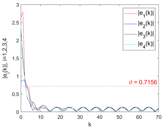
Figure 2. Error trajectories under protocol (4) with external disturbances.

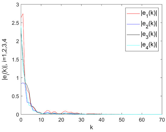
Figure 3. Error trajectories under protocol (4) without external disturbances.

To illustrate the advantages of the control scheme proposed in this paper, the norm of the system error in this study was compared with that in [18]. For the convenience of observation and comparison, it is assumed that the external disturbance is always zero. Under the same conditions, the following system parameters can be obtained in [18]:

$$K=\left[\begin{array}{cc}1& -0.5181\end{array}\right],P=\left[\begin{array}{cc}109.239& -55.046\\ -55.046& 114.236\end{array}\right].$$

The corresponding simulation results are shown in Figure 4, where control designed scheme (4) was compared with the one in [18] under the same external disturbance and uncertainty conditions. Compared with the latter, control designed scheme (4) has a faster convergence of the system error curve and exhibits a stronger anti-disturbance capability. Simultaneously, the scheme in this study eliminates the dependence on the Mahler measure of system matrix A in [18].

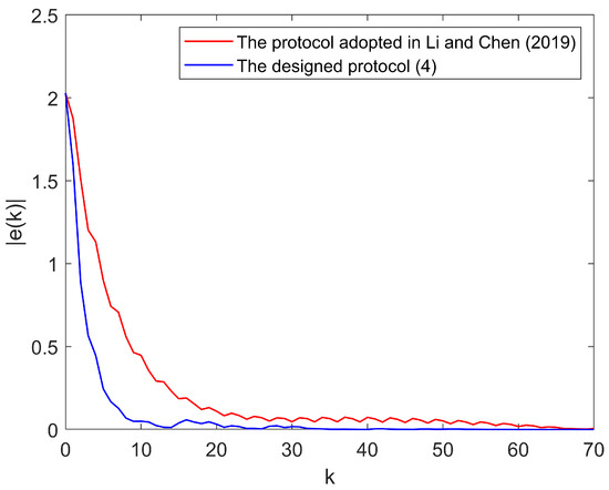
Figure 4. trajectories with protocol adopted in Li and Chen (2019) [18] and protocol (4) designed in this paper.

The better convergence speed is not attributed to the structural advantage of the protocol itself but rather to the following two key factors:

(1)

Specific tuning of the PARE parameter $\gamma$: The PARE transforms the quadratic optimal control solution of the algebraic Riccati equation in [18] into a tunable parameter $\gamma$. Notably, $\gamma$ is closely related to the pole placement of the closed-loop system, which can be flexibly adjusted by designers according to the requirements for eigenvalue distribution and dynamic response characteristics of the closed-loop system [32]. The convergence rate adjusting parameter $\gamma$ is shown in Figure 5, which leads to the fact that appropriately increasing parameter $\gamma$ can improve the controller accuracy and accelerate the error convergence. Moreover, the system maintains consensus, and the relative fluctuation in the convergence speed is limited to less than $10\%$ ($\lambda =0.919,0.964,0.9991$ for $\gamma =0.6,0.55,0.5$, respectively). This demonstrates that the proposed method is not sensitive to arbitrary tuning of $\gamma$ within the feasible range, confirming its strong parameter robustness.

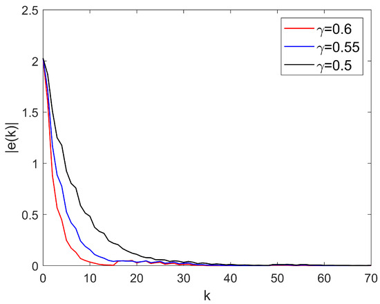Figure 5. trajectories under different $\gamma =0.6,0.55,0.5$, respectively.

(2)

Differences in theoretical analysis frameworks: While [18] derives the necessary and sufficient conditions for consensus solely based on the ARE, this paper combines the PARE with the Lyapunov stability theory and linear matrix inequality methods for consensus analysis. Specifically, the Lyapunov stability theory enables the analysis to focus more on guaranteeing the convergence performance of the system, while the LMI approach relaxes the conservativeness in parameter selection compared to the ARE-based method in [18], allowing for a larger feasible region of parameters.

In addition, to verify the feasibility of the range and robustness of $\mu$, we select $\mu =0.25,0.2,0.15$ with fixed $\gamma =0.6$ for simulation. The corresponding results are presented in Figure 6. As observed from Figure 6, for a given $\gamma$, the convergence rate slows down with the decrease in $\mu$, which reveals a positive correlation between the control gain scalar $\mu$ and the convergence rate $\lambda$. Furthermore, even though the reduction in $\mu$ reaches $25\%$, the degradation of the convergence rate is maintained within $5\%$ ($\lambda =0.9432,0.919,0.9$ for $\mu =0.25,0.2,0.15$, respectively). This result further verifies the strong parameter robustness of the proposed control strategy.

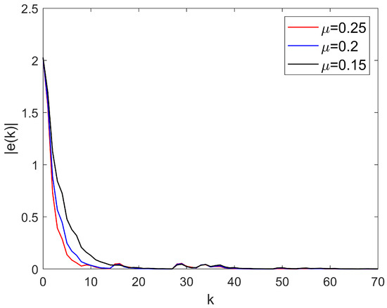
Figure 6. Error trajectories under $\mu =0.25,0.2,0.15$, respectively.

5. Conclusions

This study comprehensively considered the uncertainty factors in the system and network and studied the mean-square quasi-consensus problem of general linear discrete-time multi-agent systems. Compared to previous studies, this study established a more universal uncertainty model and derives a new lemma based on the parametric algebraic Riccati equation. Based on this, combined with the Lyapunov stability analysis method, sufficient conditions for achieving mean-square quasi-consensus were provided. Finally, numerical simulations verified the feasibility of the proposed method. Future research will consider introducing event-triggered control under uncertainties, since event-triggered control can effectively save communication, computational, and energy resources.

References

- Han, L.; Wang, Y.; Yan, Z.; Li, X.; Ren, Z. Event-triggered formation control with obstacle avoidance for multi-agent systems applied to multi-UAV formation flying. Control Eng. Pract. 2024, 153, 106105. [Google Scholar] [CrossRef]
- Hu, H.; Lyu, Y.; Fan, R.; Sui, X.; Zhan, C.; Niyato, D. Dynamic access control in multi-Layer satellite remote sensing system using multi-agent deep reinforcement learning. IEEE Trans. Wirel. Commun. 2025, 24, 5539–5555. [Google Scholar] [CrossRef]
- Yan, Z.; Han, L.; Li, X.; Dong, X.; Li, Q.; Ren, Z. Event-triggered formation control for time-delayed discrete-time multi-agent system applied to multi-UAV formation flying. J. Frankl. Inst. 2023, 360, 3677–3699. [Google Scholar] [CrossRef]
- Liu, C.; Xia, Z.; Patton, R.J. Distributed fault-tolerant consensus control of vehicle platoon systems with DoS attacks. IEEE Trans. Veh. Technol. 2024, 73, 14438–14449. [Google Scholar] [CrossRef]
- Olfati-Saber, R.; Fax, J.A.; Murray, R.M. Consensus and cooperation in networked multi-agent systems. Proc. IEEE. 2007, 95, 215–233. [Google Scholar] [CrossRef]
- Gu, Z.; Wang, X.; Wang, Z. Event-triggered control-based dynamic adaptive cooperative obstacle avoidance method for multi-aircraft. Aerosp. Sci. Technol. 2025, 168, 110892. [Google Scholar] [CrossRef]
- Lin, L.; Huang, J. Direct adaptive cooperative output regulation of unknown multi-agent systems via distributed internal model. IEEE Trans. Autom. Control 2025, 70, 7644–7651. [Google Scholar] [CrossRef]
- Chaoui, M.; Mokni, K. A discrete evolutionary Beverton–Holt population model. Int. J. Dynam. Control 2023, 11, 1060–1075. [Google Scholar] [CrossRef]
- Wang, Z.; Wang, W.; Xu, J.; Zhang, H. Leader-following consensus for discrete-time multi-agent systems with nonidentical channel fading. IEEE Trans. Autom. Control 2024, 70, 542–548. [Google Scholar] [CrossRef]
- Luo, M.; Su, H.; Zheng, W.X. Interval observer-based coordination control for discrete-time multi-agent systems. IEEE Trans. Syst. Man Cybern.-Syst. 2025, 55, 4102–4114. [Google Scholar] [CrossRef]
- Zamani, N.; Kamali, M.; Askari-Marnani, J.; Kalantari, H.; Aghdam, A.G. Fault-tolerant leader-follower controller for uncertain nonlinear multi-agent systems. IEEE Trans. Autom. Sci. Eng. 2024, 22, 9376–9387. [Google Scholar] [CrossRef]
- Zhang, L.; Zhang, H.; Xie, L. Mean-square output consensus for heterogeneous multi-agent systems over nonidentical packet loss channels. Automatica 2024, 160, 111463. [Google Scholar] [CrossRef]
- Sun, F.; Han, Y.; Wu, X.; Zhu, W.; Kurths, J. Group consensus of fractional-order heterogeneous multi-agent systems with random packet losses and communication delays. Phys. A 2024, 636, 129547. [Google Scholar] [CrossRef]
- Kato, T.; Okumura, K.; Sasaki, Y.; Yokomachi, N. Congestion mitigation path planning for large-scale multi-agent navigation in dense environments. IEEE Robot. Autom. Lett. 2025, 10, 9742–9749. [Google Scholar] [CrossRef]
- Wang, Z.; Sun, L.; Wang, H.; Hu, W.; Wang, J.; Ma, Z. Joint routing and scheduling optimization with swarm intelligence in time-sensitive networking. In Proceedings of the 2024 IEEE 99th Vehicular Technology Conference (VTC2024-Spring), Singapore, 24–27 June 2024; IEEE: New York, NY, USA, 2024; pp. 1–6. [Google Scholar]
- Li, Z.; Chen, J. Robust consensus of linear feedback protocols over uncertain network graphs. IEEE Trans. Autom. Control 2017, 62, 4251–4258. [Google Scholar] [CrossRef]
- Zelazo, D.; Bürger, M. On the robustness of uncertain consensus networks. IEEE Trans. Control Netw. Syst. 2015, 4, 170–178. [Google Scholar] [CrossRef]
- Li, Z.; Chen, J. Robust consensus for multi-agent systems communicating over stochastic uncertain networks. SIAM J. Control Optim. 2019, 57, 3553–3570. [Google Scholar] [CrossRef]
- Li, Z.; Chen, J. Robust consensus of multi-agent systems with stochastic uncertain channels. In Proceedings of the 2016 American Control Conference (ACC), Boston, MA, USA, 6–8 July 2016; IEEE: New York, NY, USA, 2016; pp. 3722–3727. [Google Scholar]
- Wu, J.; Wang, W.; Tang, W.; Xie, Y.; Nian, X. Neural networks based finite-time cluster quasi-consensus for unknown nonlinear multi-agent systems with input saturations. Neurocomputing 2025, 623, 129391. [Google Scholar] [CrossRef]
- Yuan, Q.; Chen, G.; Tian, Y.; Yuan, Y.; Zhang, Q.; Wang, X.; Liu, J. Leader-following consensus of discrete-time nonlinear multi-agent systems with asymmetric saturation impulsive Control. Mathematics 2024, 12, 469. [Google Scholar] [CrossRef]
- Wang, K.P.; Tang, Z.; Park, J.H.; Feng, J. Impulsive time window based quasi-consensus on stochastic nonlinear multi-agent systems. IEEE Trans. Netw. Sci. Eng. 2022, 9, 3602–3613. [Google Scholar] [CrossRef]
- Fu, M.; Xie, L. The sector bound approach to quantized feedback Control. IEEE Trans. Autom. Control 2005, 50, 1698–1711. [Google Scholar]
- Elia, N.; Mitter, S.K. Stabilization of linear systems with limited information. IEEE Trans. Autom. Control 2002, 46, 1384–1400. [Google Scholar] [CrossRef]
- Chen, R.; Peng, S. Leader-follower quasi-consensus of multi-agent systems with packet loss using event-triggered impulsive Control. Mathematics 2023, 11, 2969. [Google Scholar] [CrossRef]
- Guo, S.; Xie, L. Adaptive neural consensus of unknown non-linear multi-agent systems with communication noises under Markov switching topologies. Mathematics 2023, 12, 133. [Google Scholar] [CrossRef]
- Liu, S.; Huang, J. Decentralized adaptive event-triggered fault-tolerant cooperative control of multiple Unmanned aerial vehicles and unmanned ground vehicles with prescribed performance under denial-of-service attacks. Mathematics 2024, 12, 2701. [Google Scholar] [CrossRef]
- Xiao, Q.C.; Long, Y.; Su, Q.; Zhao, X.Q.; Zhong, G.X. Fault-tolerant consensus of nonlinear multi-agent systems with channel noises under multiple faults and denial-of-service attacks. Nonlinear Dyn. 2024, 112, 17205–17220. [Google Scholar] [CrossRef]
- Xie, X.; Wei, T.; Li, X. Hybrid event-triggered approach for quasi-consensus of uncertain multi-agent systems with impulsive protocols. IEEE Trans. Circuits Syst. I-Regul. Pap. 2021, 69, 872–883. [Google Scholar] [CrossRef]
- Zhu, H.; Lu, J.; Lou, J. Event-triggered impulsive control for nonlinear systems: The control packet loss case. IEEE Trans. Circuits Syst. II-Express Briefs 2022, 69, 3204–3208. [Google Scholar] [CrossRef]
- Gao, C.; Wang, Z.; He, X.; Liu, Y.; Yue, D. Differentially private consensus control for discrete-time multiagent systems: Encoding–decoding schemes. IEEE Trans. Autom. Control 2024, 69, 5554–5561. [Google Scholar] [CrossRef]
- Zhou, B. Truncated Predictor Feedback for Time-Delay Systems; Springer: Berlin/Heidelberg, Germany, 2014. [Google Scholar]
- Hengster-Movric, K.; You, K.; Lewis, F.L.; Xie, L. Synchronization of discrete-time multi-agent systems on graphs using Riccati design. Automatica 2013, 49, 414–423. [Google Scholar] [CrossRef]
Disclaimer/Publisher’s Note: The statements, opinions and data contained in all publications are solely those of the individual author(s) and contributor(s) and not of MDPI and/or the editor(s). MDPI and/or the editor(s) disclaim responsibility for any injury to people or property resulting from any ideas, methods, instructions or products referred to in the content. |
© 2025 by the authors. Licensee MDPI, Basel, Switzerland. This article is an open access article distributed under the terms and conditions of the Creative Commons Attribution (CC BY) license (https://creativecommons.org/licenses/by/4.0/).