Ship Scheduling and Refueling for Container Liner Cold Chain Shipping

Abstract

Liner shipping companies commonly pursue strategies such as forming strategic alliances and attracting new customers to strengthen competitiveness and improve operational performance. However, in the shipping of perishable goods, inadequate ship scheduling and bunker management can result in substantial customer loss and increased operational costs. This paper examines a scenario in which a large volume of perishable goods is shipped by liner ships. The specific demand characteristics of perishable goods—requiring rapid port handling and expedited shipping—are analyzed. To address these challenges, we propose a mixed-integer nonlinear programming (MINLP) model to optimize ship scheduling and refueling decisions for liner cold chain services under cooperative agreements. The model minimizes total liner shipping service costs while explicitly accounting for the decay of perishable goods. Nonlinear elements are linearized using a piecewise linear secant approximation, enabling efficient solution of the model with commercial solvers. Numerical experiments based on the AEU6 route operated by China COSCO Shipping Group validate the model and provide practical managerial insights. The results indicate that: (1) incorporating collaborative agreements can reduce total route service costs by 4.5% and total port handling costs by 7.5%, while also lowering late arrival penalties and losses from perishable goods decay; (2) joint consideration of refueling strategies and collaborative agreements improves both decision flexibility and solution accuracy; (3) the shipping of perishable goods has differentiated effects across voyage legs, highlighting the need for liner shipping companies to enhance cooperation with ports and refine bunker fuel procurement planning; and (4) it is essential to improve ship performance and appropriately design bunker fuel tank capacity to respond to dynamic changes in the shipping market.

1. Introduction

Liner shipping primarily transports containerized cargo, including manufactured goods, food products, and general consumer items, and forms a vital component of the global maritime logistics system [1]. According to Container Trades Statistics Ltd. (CTS), global annual container throughput reached 183.2 million TEUs in 2024, marking an approximate 6% increase compared to 2023 [2]. Refrigerated (reefer) trade accounts for around 6% of total international containerized transport [3], and authoritative forecasts predict that the global refrigerated container market will grow at a compound annual growth rate of approximately 8.8% between 2024 and 2030 [4]. With the rapid expansion of perishable goods shipping, refrigerated containers are capturing an increasing share of the container fleet [5].

Perishable goods transported in containers are highly sensitive to operational and environmental conditions—such as transit time, temperature, and humidity—which directly affect product integrity [6,7,8,9,10]. While the use of refrigerated units, insulated containers, and smart monitoring technologies has improved control over these factors, a significant portion of goods still suffers from spoilage. Industry data indicate that nearly one-quarter of perishable goods is lost annually due to prolonged shipping and uncontrolled temperature fluctuations [11]. Consequently, efficient ship scheduling aimed at accelerated delivery is critical to reducing the deterioration of perishable goods.

Unlike tramp shipping, liner shipping operates as a scheduled service [12], characterized by predetermined routes, designated ports of call, stable freight rates, and regular schedules [13,14]. The reliability of service at individual ports is therefore a key factor in ship scheduling, prompting liner companies to increasingly establish cooperative arrangements with terminal operators to ensure operational efficiency and minimize delays. Through such collaborations, liner companies can negotiate service time windows and handling rates with terminal operators, facilitating operational coordination and resource optimization.

Multiple operational and market factors, including service competitiveness and potential economic losses, affect the design of liner shipping schedules [15]. For highly perishable goods, maintaining product quality upon arrival is essential to customer satisfaction [16]. To minimize cargo deterioration, liner operators often adjust sailing speeds and port handling rates to improve delivery timeliness. Increasing ship speed or terminal productivity shortens voyage duration and turnaround time, thereby reducing the number of ships required on a route and lowering inventory-related and cargo depreciation costs. However, such adjustments also increase bunker fuel and handling expenses, as propulsion energy consumption generally rises with the cube of sailing speed [17].

Given substantial fuel price differences across ports, selecting appropriate refueling ports and determining refueling amounts become critical decision variables, directly influencing total shipping costs, sailing speed, port time, and operational feasibility. Motivated by these challenges, this study investigates ship scheduling and refueling strategies for container liner cold chain shipping.

Specifically, this study addresses the following key research questions:

• How can a customized methodology be developed to simulate the shipping of perishable goods, thereby enriching existing research on ship scheduling and bunker management in liner shipping?
• How can cooperation between terminal operators and liner companies be modeled through collaborative agreements to address typical challenges in cold chain shipping and propose strategies to reduce cargo decay?
• How can port service time windows, handling rates, ship arrival/departure times, and refueling amounts be optimized to enhance the stability of port–shipping company cooperation?
• How can a scalable and replicable solution method be designed to ensure both high solution quality and computational efficiency?

Accordingly, the academic contributions of this study are summarized as follows:

• This study is the first to incorporate perishable goods decay costs into refueling decisions while simultaneously embedding collaborative agreement mechanisms. Cooperative agreements are represented by multiple selectable time windows and handling rates, with sailing time and port time endogenized as decision variables. These modeling features create a bi-directional interaction between refueling strategies and ship scheduling, while the introduction of perishable goods further complicates the underlying decision-making processes, enriching existing theoretical methodologies.
• Unlike previous studies, this paper formulates the choices of time windows, handling rates, and refueling ports as binary variables within a mixed-integer nonlinear programming (MINLP) framework, enabling integrated optimization that balances multiple cost components in a unified decision structure.
• A piecewise linear secant approximation method is developed to balance solution accuracy and computational efficiency, allowing the model to be solved using commercial solvers. This approach can achieve high-quality solutions with fewer linear segments, improving overall computational performance.
• Numerical experiments are conducted to evaluate the advantages of the proposed approach over existing methods. The results provide key managerial insights for optimizing perishable goods transportation under collaborative agreements and demonstrate the superiority of the integrated scheduling–refueling framework.

The remainder of the paper is structured as follows. Section 2 reviews relevant literature. Section 3 presents a detailed problem definition, followed by the model development in Section 4. Section 5 introduces linearization techniques and derives the MILP formulation. Section 6 presents computational experiments based on a real-world liner shipping route. Finally, Section 7 concludes and discusses future research directions.

2. Literature Review

Sailing speed plays a critical role in determining bunker fuel costs, which are further influenced by fuel prices and port refueling discounts. Consequently, ship scheduling is closely intertwined with refueling strategies. This literature review is organized into three main sections: (1) ship scheduling, (2) refueling strategies, and (3) research gaps and opportunities.

2.1. Ship Scheduling

Over the past decades, extensive research has focused on optimizing ship scheduling, primarily aiming to coordinate sailing speeds, port arrival and departure times, and port handling durations [18]. Numerous studies have investigated the determination of optimal sailing speeds across voyage legs to enhance operational efficiency and reduce fuel consumption [19,20]. Building on this, some studies introduced time window constraints to optimize speed while improving service levels [21]. With growing attention to environmental sustainability, recent research has increasingly addressed green ship scheduling. In this section, we review relevant work on green ship scheduling, uncertainty management, schedule recovery, collaborative agreements, and the handling of different cargo types.

2.1.1. Green Ship Scheduling

Kontovas [22] explored green ship routing and scheduling, identifying key parameters for modeling and estimating emissions and fuel consumption. Psaraftis and Kontovas [23] developed models for selecting optimal speeds across alternative routes, integrating these determinants into shipowner or charterer decision-making. Fagerholt et al. [24] and Fagerholt and Psaraftis [25] analyzed the impact of Emission Control Areas (ECAs) on sailing paths and speeds, addressing the so-called ECA refraction problem. Moving beyond single-objective optimization, Mansouri et al. [26] applied a multi-objective framework to evaluate long-term environmental sustainability. Song et al. [27] addressed integrated tactical planning by simultaneously determining fleet size, maximum speed, and schedules using a simulation-based non-dominated sorting genetic algorithm. Dulebenets [28] linearized reciprocal speeds to balance solution accuracy and efficiency, while Zhang et al. [29] analyzed optimal speeds under fuel switching and scrubber installation strategies. Sun et al. [30] studied optimal speed decisions for liner alliances under maritime emission trading systems.

2.1.2. Uncertainty Operations

Port handling operations, sailing durations, and port demands are inherently uncertain, making stochastic analysis critical for liner shipping. Notteboom [17] highlighted that port congestion and resource constraints cause schedule unreliability. Vernimmen et al. [31] found that schedule unreliability increases inland shipping costs and safety stock levels. Fuzzy set theory has been applied to handle uncertainties in port time, sailing time, and port demand [32]. Qi and Song [33] incorporated port time uncertainty into liner scheduling using a simulation-based stochastic approximation. Wang and Meng [34] examined ship schedule design under uncertain waiting and handling times, including sailing and port operation uncertainties. Wang and Meng [35], Wang [36] determined ship sequences considering container capacity and port demand to minimize delays. Li et al. [37] optimized the Northern Sea Route schedule under weather and ocean uncertainties, considering delay penalties. Zhang et al. [38] addressed arrival and departure time uncertainties to reduce total port waiting time and improve schedule robustness. Xia et al. [39] achieved synergistic efficiency and low-carbon operation by jointly optimizing ship scheduling and speed reduction. Zhen et al. [40] designed ship schedules under ECAs using green technologies and biofuels while coordinating port cargo allocation. Ganjian et al. [41] conducted coordinated energy management and scheduling optimization for fuel-cell-powered ships.

2.1.3. Ship Schedule Recovery

Disruptions in operations necessitate schedule recovery strategies. Brouer et al. [42] proposed four recovery strategies—delays, swaps, cancelations, and speed adjustments—balancing cost, network integrity, and service performance, with port swaps and skips proving effective under severe delays [43]. Li et al. [44] extended these strategies to account for probabilistic variations and rare extreme events. Compliance with International Maritime Organization (IMO) regulations in ECAs adds complexity, leading Abioye et al. [45] to formulate an MINLP model minimizing profit loss from planned interruptions. Elmi et al. [46] developed a multi-objective optimization model aiming to minimize both total port arrival delays and profit losses induced by disruptions. Extending this work, Elmi et al. [47] incorporated slow-steaming incentive programs and ECA-related constraints into a refined multi-objective schedule recovery model. In a related study, Zheng et al. [48] proposed an event-triggered model predictive control framework for dynamic recovery. Furthermore, Zhao et al. [49] integrated heterogeneous ship deployment with Conditional Value-at-Risk (CVaR) to quantify uncertainty-related risks.

2.1.4. Collaborative Agreements

Collaborative mechanisms with terminals, including flexible time windows (TWs) and multiple handling rates, have proven effective in reducing bunker costs and improving operational coordination. Wang et al. [50] developed a mixed-integer nonlinear model with multiple time window options at each port, demonstrating practical applicability. Alharbi et al. [51] extended scheduling under multiple ship arrival time windows, and Liu et al. [52] proposed a mechanism where terminals provide adjustable handling rates compensated by shipping companies, thereby reducing bunker consumption. Dulebenets [53] and Dulebenets et al. [54] proposed comprehensive cooperative frameworks with multi-TW and multi-rate options, facilitating sustainable and environmentally conscious ship schedules via exact multi-objective optimization.

2.1.5. Transportation of Perishable Goods

Significant progress has been made in road logistics regarding perishable goods, highlighting the importance of mitigating cargo deterioration [55,56,57]. However, research on time-sensitive cargo in maritime transport remains limited. Wang et al. [58] studied optimal scheduling with time-sensitive requirements, modeling cargo decay as a continuous decreasing function of shipping time and proposing a branch-and-bound solution method. Building on this, Wang et al. [59] addressed container distribution with shipping demand as a non-increasing function of transit time to determine the proportion of demand satisfied across a network. Dulebenets and Ozguven [5] simulated the decay of perishable goods on ships and developed ship scheduling models incorporating perishability. The key differences between maritime and road-based studies motivate this research, aiming to extend operations research applications to liner shipping.

Table 1 summarizes the literature, highlighting that ship scheduling is closely linked to bunker costs, environmental regulations, operational uncertainties, and terminal collaboration. Early studies focused on speed optimization for fuel efficiency, while recent research emphasizes green technologies, emission trading, and robust scheduling under uncertainty. Collaborative strategies, including flexible time windows and adjustable handling rates, have proven effective in reducing costs and enhancing coordination. Although research on perishable goods in maritime shipping remains limited, it presents a promising direction for integrating time-sensitive considerations into liner shipping operations.

Table 1. Comparison of key literature on ship scheduling.

Reference	Focus	Method/Model	Key Findings
Kontovas [22]	Green ship routing and scheduling	Parameter identification	Laying foundation for estimating emissions and fuel consumption
Psaraftis & Kontovas [23]	Optimal sailing speeds	Routing scenario model	Integrating key determinants into shipowner decision-making
Fagerholt et al. [24]; Fagerholt & Psaraftis [25]	ECA speed optimization	Analytical and optimization	Minimizing bunker cost and examining ECA effects
Mansouri et al. [26]	Multi-objective scheduling	Multi-objective framework	Exploring long-term environmental sustainability
Song et al. [27]	Tactical planning	Simulation-based GA	Optimizing fleet size, maximum speed, and schedule
Dulebenets [28]	Green scheduling	Linearization of reciprocal speed	Applying collaborative mechanisms to reduce emissions
Zhang et al. [29]; Sun et al. [30]	ECA and emission trading	Optimal speed analysis	Assessing fuel switching, scrubber installation, and alliance strategies
Notteboom [17]; Vernimmen et al. [31]	Scheduling under uncertainty	Observational/empirical	Addressing port congestion and inland cost increase
Qi & Song [33]; Wang & Meng [34,35,36]	Stochastic scheduling	Simulation and uncertainty models	Strengthening schedule robustness
Li et al. [37]; Zhang et al. [38]	NSR and unpredictable events	Optimization under uncertainty	Reducing port waiting time and enhancing schedule stability
Xia et al. [39]; Zhen et al. [40]; Ganjian et al. [41]	Green tech and low-carbon operation	Joint scheduling and speed reduction	Integrating biofuels, green technologies, and energy management
Brouer et al. [42]; Li et al. [44]; Abioye et al. [45]; Elmi et al. [46,47]; Zheng et al. [48]; Zhao et al. [49]	Schedule recovery and disruptions	MINLP model, multi-objective, event-triggered	Developing recovery strategies and quantifying uncertainty risks
Wang et al. [50]; Alharbi et al. [51]; Liu et al. [52]; Dulebenets [53,54]	Collaborative scheduling	MINLP model	Incorporating multiple time windows and handling rates to reduce bunker cost
Wang et al. [58,59]; Dulebenets & Ozguven [5]	Perishable goods	Simulation and optimization	Modeling perishable good decay and optimizing scheduling

Source: Compiled by the authors; no copyright issues are involved.

2.2. Refueling Strategy

While most previous studies focus on ship scheduling with the goal of minimizing total operational costs, unrealistic fuel price settings can significantly affect sailing speeds, handling rates, and fleet deployment decisions. Refueling decisions—specifically, where and how much to refuel—directly influence total bunker costs by leveraging spatial fuel price differences across ports. These decisions, in turn, impact ship schedules, handling costs, and overall fuel consumption. Therefore, refueling strategies must be integrated into the decision-making process alongside sailing time, port time, and ship deployment. This section reviews key literature on refueling optimization.

2.2.1. Refueling Decisions and Adaptive Policies

Refueling decisions critically affect bunker costs, which cascade into ship scheduling, handling costs, and sailing speeds. Kim et al. [60] optimized refueling along liner routes, demonstrating the environmental benefits of slow steaming. Yao et al. [61] emphasized the joint optimization of refueling port selection, fuel amounts, and speed adjustments. Kim [62] applied a Lagrangian heuristic to determine optimal speeds and refueling ports. Sheng et al. [63] introduced a multi-stage model that accounts for stochastic fuel prices, enabling adaptive refueling decisions over time. Subsequently, Sheng et al. [64] proposed an (s, S) policy for refueling under fuel price and consumption uncertainties. Meng et al. [65] extended these methods to tramp shipping, incorporating cargo heterogeneity and port-dependent fuel prices using a branch-and-price (B&P) algorithm. Wang and Meng [66] analyzed worst-case bunker consumption under speed uncertainty, while De et al. [67] addressed stochastic fuel consumption and price variability using threshold-based policies and dynamic programming.

2.2.2. Integrated Refueling Strategies and Operational Applications

Aydin et al. [68] studied speed optimization under stochastic port times using dynamic programming. Wang and Chen [69] studied the refueling strategy under low carbon background. Wang et al. [70] studied the refueling strategy and freight revenue considering ship capacity and load. Wang et al. [71] examined the impacts of alternative refueling ports along shipping routes, optimal port layover (OPL) refueling times, detour distances, and overall fuel price levels on voyage costs for shipping companies. Du and Wu [72] proposed a stochastic dynamic programming framework optimizing fleet deployment, refueling ports, methods, amounts, and sailing speeds under ECA constraints. Wu et al. [73] examined LNG dual-fuel ships under carbon intensity indicator (CII) rating limits and fuel price uncertainty, and Gao et al. [74] analyzed methanol dual-fuel ships. Despite these advances, most studies overlook the effects of port handling rates and cargo type, which remain unaddressed in current research and are considered in this paper.

The literature demonstrates that refueling strategies play a pivotal role in bunker costs, ship scheduling, and overall operational efficiency. Prior research primarily addresses the optimization of refueling port selection, fuel amounts, and sailing speeds under stochastic fuel prices, variable port times, and environmental regulations, using heuristic algorithms, branch-and-price methods, integer programming, and dynamic programming. However, the integration of port handling rates, cargo perishability, and collaborative agreements remains limited, highlighting a clear gap. This gap motivates the development of a comprehensive framework that jointly considers bunker fuel management and ship scheduling, as presented in this study.

2.3. Summary of Literature Review

Overall, the literature review indicates substantial progress in ship scheduling and refueling strategy research, providing a strong theoretical foundation for this study. Table 2 summarizes key studies, revealing the lack of an integrated framework that simultaneously accounts for refueling, collaborative agreements, and cargo perishability under variable sailing and port times, with the goal of minimizing total shipping costs. Investigating the interdependencies and cascading effects among these factors is essential for advancing both theoretical methodologies and managerial insights in liner shipping. To address this gap, this study develops a comprehensive model that incorporates these factors and implements an efficient solution approach, aiming to uncover the intrinsic relationships among interrelated elements and their impact on operational performance.

Table 2. Overview of the literature in liner shipping.

Reference	Sailing Time	Port Time	Objective	Solution Approach	Refueling Considerations	Collaborative Agreements Considerations	Perishability Considerations
Fagerholt et al. [24]; Fagerholt & Psaraftis [25]	V	F	Minimize the total cost	CPLEX	N/A	N/A	N/A
Qi & Song [33]	V	U	Minimize the total cost	Stochastic approximation	N/A	N/A	N/A
Wang & Meng [34]	U	U	Minimize the total cost	A cutting-plane algorithm	N/A	N/A	N/A
Wang & Meng [35]	V	U	Minimize the total cost	Sample average approximation	N/A	N/A	N/A
Wang et al. [50]	V	F	Minimize the total cost	Iterative optimization algorithm	N/A	Multiple time windows	N/A
Alharbi et al. [51]	V	F	Minimize the total cost	Iterative optimization algorithm	N/A	Multiple time windows	N/A
Dulebenets [53,54]	V	V	Minimize the total cost	CPLEX	N/A	A	N/A
Dulebenets & Ozguven [5]	V	V	Minimize the total cost	CPLEX	N/A	N/A	A
Wang and Meng [66]	V	F	Minimize the total cost	CPLEX	A	N/A	N/A
Wang and Chen [69]	V	F	Minimize the total cost	CPLEX	A	N/A	N/A
Wu et al. [73]	V	F	Minimize the total cost	CPLEX	A	N/A	N/A
Gao et al. [74]	V	F	Minimize the total cost	Intlinprog tool	A	N/A	N/A
This paper	V	V	Minimize the total cost	CPLEX	A	A	A

Notes: F—fixed; V—variable; U—uncertain; A—applicable; N/A—not applicable. Source: Compiled by the authors; no copyright issues are involved.

3. Problem Description

This section presents a comprehensive problem description, encompassing the following key components: (1) collaborative agreement mechanisms, (2) port handling cost, (3) late arrival penalty, (4) container inventory cost, (5) shipping of perishable goods, (6) refueling, and (7) interdependencies among decisions.

3.1. Collaborative Agreement Mechanisms

Increasing vertical integration between terminal operators and shipping companies has fostered strategic collaboration that benefits both parties. Terminal operators can secure investments, ensure stable demand, and allocate port resources more effectively, while shipping companies gain enhanced support, including more flexible port time windows and faster access to handling equipment. From a tactical planning perspective, these agreements offer shipping companies multiple selectable port time windows and container handling rate options, providing greater scheduling flexibility. Higher handling rates, however, consume more resources and incur higher costs. Modeling these agreements introduces additional complexity in berth allocation and port time assignment, particularly when combined with considerations such as perishable goods and fuel pricing, which jointly influence refueling strategies and overall scheduling. In this model, each port is associated with multiple time windows and container handling rate options, represented by binary selection variables. Ship bunker levels and voyage timing are integrated to allow coordinated optimization of both refueling and scheduling.

Formally, the set of ports to be called by the ships is denoted as $I=\left\{1,2,\dots ,n\right\}$. Each ship sails between two consecutive ports $i$ and $i+1$, along leg $i$. A collaborative agreement is defined, comprising three essential components: (1). the set of available ship arrival time windows $T_i=\left\{1,2,\dots ,m_i\right\}$; (2). the set of start times $S_{it}=\left\{1,2,\dots ,g_{it}\right\}$, $i\in I$, $t\in T_i$ and end times $E_{it}=\left\{1,2,\dots ,o_{it}\right\}i$, $i\in I$, $t\in T_i$ for each window; and (3). the set of associated handling rates $H_{it}=\left\{1,2,\dots ,w_{it}\right\}$, $i\in I$, $t\in T_i$.

Each time window is characterized by its start time $T{W}_{its}^S$ and end time $T{W}_{ite}^E$, within which the ship is required to arrive. The terminal operator is assumed to provide $m$ available arrival TWs, $g$ start times, $o$ end times, and $w$ handling rates associated with each TW. These parameters jointly define the collaborative agreement, under which terminal operators offer $m\cdot g\cdot o$ arrival time TWs, $w$ handling rate options. The duration of a time window varies across ports, typically ranging from 1 to 3 days. As illustrated in Figure 1, at port $i$, 3 start and 3 end times for each TW $t$ are provided by the terminal operator, corresponding to $3\cdot 3\cdot m=9m$ available arrival time windows in total. It is assumed that ships must arrive within the designated time window, as early or late arrivals may result in operational inefficiencies or penalty costs, as further discussed in Section 3.3 [53].

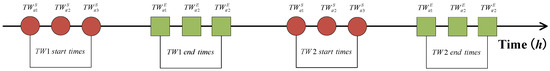
Figure 1. Illustration of 3 start times and 3 end times at a port. Source: Drawn by the authors; no copyright issues are involved.

As shown in Figure 2, the ship selects time window $\left[T{W}_{1t3}^S,T{W}_{1t1}^E\right]$ at port 1, time window $\left[T{W}_{2t2}^S,T{W}_{2t1}^E\right]$ at port 2, and time window $\left[T{W}_{3t2}^S,T{W}_{3t1}^E\right]$ at port 3. These choices determine sailing and port times, directly shaping the ship schedule and influencing refueling decisions.

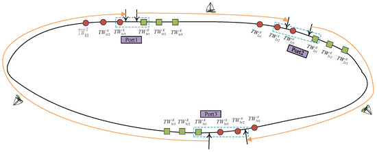
Figure 2. Schematic diagram of a ship calling at 3 ports and selecting time windows. Source: Drawn by the authors; no copyright issues are involved.

3.2. Port Handling Cost

Each selected time window corresponds to a handling rate, denoted as $H{P}_{ith}$, $i\in I$, $t\in T_i$, $h\in H_{it}$ (TEUs/h), representing the handling productivity during TW $t$ at port $i$. The handling productivity varies across ports and time windows, depending on the availability and capacity of handling equipment. The handling time is estimated by the total number of containers processed, $D_i$ (TEUs), and the handling rate $h$, expressed as: $t_i^b={\displaystyle \sum _{t\in T_i}{\displaystyle \sum _{h\in H_{it}}{y}_{ith}\frac{D_i}{H{P}_{ith}}}}$ (h). The handling cost, denoted as $C_{ith}^{hc}$, $i\in I$, $t\in T_i$, $h\in H_{it}$ (USD/TEU), is influenced by ports of call, the selected time window, and the chosen handling rate. Even under identical handling productivity, handling cost may differ across ports due to variations in labor charges, equipment utilization efficiency, and port congestion levels. Generally, higher handling productivity is associated with higher handling costs because of the additional resources and operational intensity required during peak service periods. The total handling cost can be calculated as: $THC={\displaystyle \sum _{i\in I}{\displaystyle \sum _{t\in T_i}{\displaystyle \sum _{h\in H_{it}}{C}_{ith}^{hc}{y}_{ith}{D}_i}}}$, where $y_{ith}$ is a binary decision variable equal to 1 if $H{P}_{ith}$ is selected, and 0 otherwise.

3.3. Late Arrival Penalty

The following defines ship late arrivals at ports and the corresponding late arrival penalty. In practical operations, ship arrivals at the next port can occur in 3 possible timing scenarios, as illustrated in Figure 3. A ship should arrive at port $i$ within TW $t$. If a ship arriving before the start of the selected TW $t$, it must wait in the anchorage or designated holding area until the time window starts. Conversely, if a ship arrives at the port beyond the end of the selected TW $t$, additional penalty charges are imposed. Late arrivals beyond the end of TW $t$ may lead to significant disruption of ports, potentially resulting in handling delays of subsequent ships. The total penalty cost associated with late ship arrivals can be estimated as: $TLC={\displaystyle \sum _{i\in I}{C}_i^{lc}{t}_i^l}$, where $C_i^{lc}$ represents the unit penalty for delayed arrival at port $i$ (USD/h), and $t_i^l$ denotes the total duration of delay at port $i$ (h).

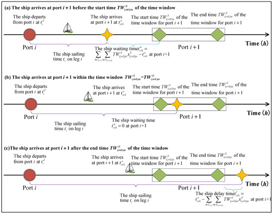
Figure 3. Three possible ship arrival times at the subsequent port. Source: Drawn by the authors; no copyright issues are involved.

3.4. Container Inventory Cost

An efficient ship scheduling plan must consider the container inventory cost, and the specific definitions are introduced below. In general, a higher sailing speed results in a shorter voyage duration, thereby reducing the inventory cost. The inventory cost depends primarily on the total sailing time and the number of containers shipped. The total inventory cost can be expressed as follows [66]: $TIC=C^{ic}{\displaystyle \sum _{i\in I}{Q}_i{t}_i}$, where $C^{ic}$ denotes the unit inventory cost (USD/TEU/h), $Q_i$ is the number of containers shipped on leg $i$ (TEUs), and $t_i$ is the sailing time on leg $i$ (h).

3.5. Shipping of Perishable Goods

The decay of perishable goods exhibits a cumulative time effect, with the rate of quality loss accelerating as shipping time increases. As a result, quality degradation follows a nonlinear, progressively accelerating pattern. Based on the physical and biochemical characteristics of perishable goods, and consistent with findings in the logistics and cold-chain literature [5,7,8,75], the quality of a perishable good type $k$ after a total shipping duration $t_{ijk}$ is modeled using an exponential function. In practical ship scheduling, when a large volume of perishable goods is shipped on specific legs, ships often increase sailing speed and select higher handling rates at ports to minimize port time. These operational adjustments, in turn, affect bunker fuel consumption, refueling decisions, and overall scheduling, highlighting the strong interdependence between cargo perishability, ship scheduling, and refueling strategies.

In this study, the set of perishable good types $K=\left\{1,\dots ,r\right\}$ is defined. For each perishable good type $k,k\in K$, the corresponding set of calling ports is denoted as $P_{ijk}=\left\{1,\dots ,n_{ijk}\right\}$. The change in quality of good type $k$ after a total shipping duration $t_{ijk}$ can be expressed as: $h\left(t_{ijk}\right)=1-e^{-{\delta }_k{t}_{ijk}} \forall i,j\in I i\ne j \forall k\in K$, where $e^{-{\delta }_k{t}_{ijk}}$ denotes the remaining quality of good type $k$ after shipping (%), $t_{ijk}$ represents the shipping time of good type $k$ (h), and ${\delta }_k$ represents the decay rate of good type $k$ (%/h).

3.6. Refueling

A fleet of homogeneous ships characterized by similar technical and operational parameters is assumed to be deployed [20,34,35,50]. Following established findings in the literature [20], the ship bunker consumption rate is represented as a power function of its sailing speed, formulated as: $g\left(v_i\right)={\displaystyle \frac{F_D}{24}} {\left({\displaystyle \frac{v_i}{V_D}}\right)}^3 \forall i\in I$, where $g\left(v_i\right)$ denotes the bunker fuel consumption rate at leg $i$ (tons/h), $v_i$ represents the sailing speed (knots), $V_D$ is the design sailing speed (knots); and $F_D$ is the daily bunker consumption at $V_D$ (tons/day). The fuel amount remaining upon arrival at port $i$ is denoted by $z_i^1$, while the fuel inventory level upon departure from the same port is $z_i^2$. Their relationship can be expressed as: $z_{i+1}^1=z_i^2-g\left(v_i\right) \forall i\in I, i<n$, $z_1^1=z_n^2-g\left(v_n\right)$. where $z_i$ represents the refueling amount at port $i$ (tons), and can be calculated by: $z_i=z_i^2 - z_i^1$.

In general, bunker fuel prices vary considerably across ports and may include amount-based discounts depending on the amount purchased, as illustrated in Figure 4 [66]. To reflect this pricing structure, the bunker cost is approximated as follows:

$$f\left(z_i\right)=\left\{\begin{array}{cc}{C}_i^{f0}{z}_i\hfill & \hfill 0\le z_i\le W_i^1\hfill \\ C_i^{f0}\left[W_i^1+{\lambda }_i^1\left(z_i-W_i^1\right)\right]\hfill & \hfill W_i^1<z_i\le W_i^2\hfill \\ C_i^{f0}\left[W_i^1+{\lambda }_i^1\left(W_i^2-W_i^1\right)+{\lambda }_i^2\left(z_i-W_i^2\right)\right]\hfill & \hfill W_i^2<z_i\le W\hfill \end{array}\right.$$

where $C_i^{f0}$ denotes the regular fuel price at port $i$ (USD/ton), ${\lambda }_i^1$ and ${\lambda }_i^2$, $0<{\lambda }_i^2\le {\lambda }_i^1\le 1$ represent the price discount factors corresponding to different purchasing levels (%), and $W_i^1$ and $W_i^2$, $W_i^1\le W_i^2$ represent the refueling amount thresholds at which discounted fuel prices become applicable (tons).

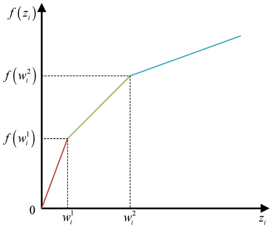
Figure 4. Bunker cost function. Source: Drawn by the authors; no copyright issues are involved.

Each refueling operation requires dedicated equipment and personnel, incurring a fixed service charge. Therefore, the bunker cost can be expressed as: $TBC={\displaystyle \sum _{i\in I}\left[E{b}_i+f\left(z_i\right)\right]}$. where $E$ represents fixed cost of ship refueling (USD), and $b_i$ represents a binary decision variable indicating if refueling occurs at that port.

3.7. Interdependencies Among Decisions

Figure 5 illustrates the relationships among the key elements of the voyage. Firstly, cooperation agreement mechanisms, fuel prices at different ports, ship characteristics, and cargo attributes jointly affect the various cost components during the voyage. Secondly, these costs influence the at-sea sailing time (i.e., speed), port time, selection of refueling ports, and refueling amounts. Thirdly, these effects directly lead to adjustments in shipping-related times and refueling strategies, with ship scheduling and refueling decisions mutually interacting with each other. Finally, the optimal ship schedule and refueling strategy are obtained. It is worth noting that the optimal solution may, in turn, affect the overall cost of liner shipping services.

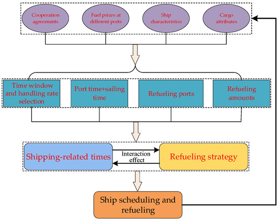
Figure 5. Interdependencies among decisions. Source: Drawn by the authors; no copyright issues are involved.

4. Model Formulation

To support the modeling process, this study adopts a set of fundamental assumptions grounded in actual shipping operations and established research (Table 3). These assumptions are designed to simplify the problem while preserving the key characteristics of cold chain shipping, ensuring that the model accurately reflects the operational realities and challenges of the industry.

Table 3. Basic assumptions.

No	Assumption
1	All container ships deployed on the liner route are of the same type
2	Port calls and their visiting sequence are predetermined
3	Sailing speed on each leg is fixed
4	Ship departure frequency on the liner route is weekly
5	Expected fuel prices at each port remain constant over the planning period
6	Change in quality of perishable goods follows an exponential relationship with time

Source: Compiled by the authors; no copyright issues are involved.

Based on the aforementioned assumptions, this section introduces the notation required by the model and then presents a MINLP model tailored to the ship scheduling and refueling for liner cold chain shipping under cooperative agreements, as shown in Table 4.

Table 4. Notation.

Notation Type	Notation	Explanation
Sets	$I=\left\{1,2,\dots ,n\right\}$	Set of ports
	$K=\left\{1,\dots ,r\right\}$	Set of perishable good types
	$T_i=\left\{1,2,\dots ,m_i\right\}$$, i\in I$	Set of available arrival TWs of port $i$
	$H_{it}=\left\{1,2,\dots ,w_{it}\right\}$$, i\in I$$, t\in T_i$	Set of available handling rates of port $i$ during TW $t$
	$S_{it}=\left\{1,2,\dots ,g_{it}\right\}$$, i\in I$$, t\in T_i$	Set of start times for TW $t$ of port $i$
	$E_{it}=\left\{1,2,\dots ,o_{it}\right\}$$, i\in I$$, t\in T_i$	Set of end times for TW $t$ of port $i$
	$P_{ijk}=\left\{1,\dots ,n_{ijk}\right\}$$, i,j\in I, i\ne j$$, k\in K$	Set of ports called by the ship when shipping perishable good type $k$
Parameters	$T{W}_{its}^S$$, i\in I$$, t\in T_i$$, s\in S_{it}$	Start time $s$ of TW $t$ at port $i$ (h)
	$T{W}_{ite}^E$$, i\in I$$, t\in T_i$$, e\in E_{it}$	End time $e$ of TW $t$ at port $i$ (h)
	$H{P}_{ith}$$, i\in I$$, t\in T_i$$, h\in H_{it}$	Handling productivity (TEUs/h)
	$C^{oc}$	Weekly operational cost of a ship (USD/week)
	$C_i^{f0}$$, i\in I$	Unit bunker fuel price at port $i$ (USD/ton)
	$C^{ic}$	Unit container inventory cost (USD/TEU/h)
	$C_k^d$$,k\in K$	Decay cost per unit quality decay of good type $k$ (USD/%)
	$C_i^{lc}$$, i\in I$	Unit penalty for late ship arrival at port $i$ (USD/h)
	$C_{ith}^{hc}$$, i\in I$$, t\in T_i$$, h\in H_{it}$	Unit handling cost (USD/TEU)
	$L_i$$, i\in I$	Distance of leg $i$
	$Q_i$$, i\in I$	Container amount shipped at leg $i$ (TEUs)
	$D_i$$, i\in I$	Container handled at port $i$ (TEUs)
	$I_0$	Minimum fuel inventory at the beginning (tons)
	$E$	Fixed cost of ship refueling (USD)
	$W$	Ship bunker tanker maximal capacity (tons)
	$W_i^1$$, i\in I$	Refueling amount thresholds at which the first fuel price discount becomes applicable (tons)
	$W_i^2$$, i\in I$	Refueling amount thresholds at which the second fuel price discount becomes applicable (tons)
	${\lambda }_i^1$$, i\in I$	$\mathrm{Price} \mathrm{discount} \mathrm{factor} \mathrm{of} \mathrm{bunker} \mathrm{fuel} \mathrm{within} \left(W_i^1,W_i^2\right]$ (%)
	${\lambda }_i^2$$, i\in I$	$\mathrm{Price} \mathrm{discount} \mathrm{factor} \mathrm{of} \mathrm{bunker} \mathrm{fuel} \mathrm{exceeding} W_i^2$ (%)
	${\delta }_k$$, k\in K$	Decay rate of perishable good type $k$ (%/h)
	$R_{ijk}$$, i,j\in I, i\ne j$$, k\in K$	Amount of good type $k$ shipped from port $i$ to $j$ (TEU)
	$P^{\max }$	Limitations of refrigerated receptacle sockets on ships (unit)
	$V_D$	Design sailing speed (knots)
	$F_D$	Bunker consumption at design speed (tons/day)
	$V^{\min }$	Minimum ship sailing speed (knots)
	$V^{\max }$	Maximum ship sailing speed (knots)
Decision Variables	$x_{it}^{TW}$, $i\in I$, $t\in T_i$	Binary variable, $x_{it}^{TW}=1$ when TW $t$ of port $i$ is selected, 0 otherwise
	$x_{its}^S$, $i\in I$, $t\in T_i$, $s\in S_{it}$	Binary variable, $x_{its}^S=1$ when start time $s$ of TW $t$ for port $i$ is selected, 0 otherwise
	$x_{ite}^E$, $i\in I$, $t\in T_i$, $e\in E_{it}$	Binary variable, $x_{ite}^E=1$ when end time $e$ of TW $t$ for port $i$ is selected, 0 otherwise
	$y_{ith}$, $i\in I$, $t\in T_i$, $h\in H_{it}$	Binary variable, $y_{ith}=1$ when handling rate $h$ of TW $t$ for port $i$ is selected, 0 otherwise
	$v_i$, $i\in I$	Sailing speed of leg $i$ (knots)
	$m$	Number of ships deployed (Vessels)
	$b_i$, $i\in I$	Binary variable, $b_i=1$ when the ship refueling at port $i$, 0 otherwise
	$z_i$, $i\in I$	Amount of bunker purchased at port $i$ (tons)
Auxiliary Variables	$t_i$$, i\in I$	Ship sailing time of leg $i$ (h)
	$t_i^w$$, i\in I$	Ship waiting time at port $i$ (h)
	$t_i^l$$, i\in I$	Ship late arrival time at port $i$ (h)
	$t_i^a$$, i\in I$	Ship arrival time at port $i$ (h)
	$t_i^d$$, i\in I$	Ship departure time from port $i$ (h)
	$t_i^b$$, i\in I$	Ship handling time at port $i$ (h)
	$z_i^1$$, i\in I$	Bunker levels at port $i$ before refueling (tons)
	$z_i^2$$, i\in I$	Bunker levels at port after refueling $i$ (tons)
	$g\left(v_i\right)$$, i\in I$	$\mathrm{Bunker} \mathrm{consumption} \mathrm{function} \mathrm{as} \mathrm{sailing} \mathrm{speed} v_i$
	$f\left(z_i\right)$$, i\in I$	Bunker cost function
	$p_i$$, i\in I$	Number of refrigerated receptacle sockets occupied when the ship arrives at port $i$ (unit)
	$t_{ijk}$$, i,j\in I, i\ne j$$, k\in K$	Total shipping time of perishable good type $k$ (h)
	$h\left(t_{ijk}\right)$$, i,j\in I, i\ne j$$, k\in K$	Function representing the total quality change in perishable good type $k$ from port $i$ to $j$

In view of this, model [M1] is formulated as follows:

The objective function (1) aims to minimize the total service cost.

The first term accounts for ship operational costs, while the final term represents the total decay cost associated with the decay of perishable goods. Additionally, the model incorporates variable costs arising from bunker fuel consumption, container handling and inventory, and ship delays, all of which are directly influenced by scheduling decisions.

$$\min F_1=\left\{C^{oc}m+{\displaystyle \sum _{i\in I}\left[E{b}_i+f\left(z_i\right)\right]}+{\displaystyle \sum _{i\in I}{\displaystyle \sum _{t\in T_i}{\displaystyle \sum _{h\in H_{it}}{C}_{ith}^{hc}{D}_i{y}_{ith}+C^{ic}{\displaystyle \sum _{i\in I}{t}_i{Q}_i}+{\displaystyle \sum _{i\in I}{C}_i^{lc}{t}_i^l}+{\displaystyle \sum _{i\in I}{\displaystyle \sum _{j\in I:j\ne i}{\displaystyle \sum _{k\in K}{C}_k^d{R}_{ijk}h\left(t_{ijk}\right)}}}}}}\right\}$$

(1)

The constraints of model [M1] are introduced as follows:

(1) Constraints (2)–(8) represent the constraints related to the collaborative agreement mechanism. Specifically, Constraint (2) enforces that the ship can only select one TW. For example, if $x_{11}^{TW}=1$, it indicates that the time window 1 at port 1 is selected. Constraints (3) and (4) and (5) and (6) ensure that exactly one start time and one end time are chosen, respectively. Constraints (7) and (8) ensure that the ship selects only one handling rate.

$${\displaystyle \sum _{t\in T_i}{x}_{it}^{TW}}=1,\forall i\in I$$

(2)

$${\displaystyle \sum _{t\in T_i}{\displaystyle \sum _{s\in S_{it}}{x}_{its}^S}}=1,\forall i\in I$$

(3)

$$x_{its}^S\le x_{it}^{TW},\forall i\in I; \forall t\in T_i; \forall s\in S_{it}$$

(4)

$${\displaystyle \sum _{t\in T_i}{\displaystyle \sum _{e\in E_{it}}{x}_{ite}^E}}=1,\forall i\in I$$

(5)

$$x_{ite}^E\le x_{it}^{TW},\forall i\in I; \forall t\in T_i; \forall e\in E_{it}$$

(6)

$${\displaystyle \sum _{t\in T_i}{\displaystyle \sum _{h\in H_{it}}{y}_{ith}}}=1,\forall i\in I$$

(7)

$$y_{ith}\le x_{it}^{TW},\forall i\in I; \forall t\in T_i; \forall h\in H_{it}$$

(8)

(2) Constraints (9)–(18) are the constraints related to ship scheduling time. Specifically, Constraint (9) calculates the sailing time, while Constraint (10) determines the port handling time. Constraint (11) computes the total shipping time for each type of perishable good, including both sailing and handling times, between its origin and destination ports. Constraint (12) defines the ship departure time, and Constraint (13) evaluates any late arrival. Constraints (14) and (15) estimate the ship waiting time before service begins, while Constraints (16) and (17) calculate ship arrival time at ports. Finally, Constraint (18) ensures that the weekly service frequency is maintained.

$$t_i={\displaystyle \frac{L_i}{v_i}}, \forall i\in I$$

(9)

$$t_i^b={\displaystyle \sum _{t\in T_i}{\displaystyle \sum _{h\in H_{it}}{y}_{ith}\frac{D_i}{H{P}_{ith}}}},\forall i\in I$$

(10)

$$t_{ijk}={\displaystyle \sum _{s\in P_{ijk}}{t}_s^b}+{\displaystyle \sum _{s\in P_{ijk}:s\ne n_{ijk}}{t}_s},\forall i,j\in I, i\ne j;\forall k\in K$$

(11)

$$t_i^d=t_i^a+t_i^b+t_i^w,\forall i\in I$$

(12)

$$t_i^l\ge t_i^a-{\displaystyle \sum _{t\in T_i}{\displaystyle \sum _{e\in E_{it}}T{W}_{ite}^E{x}_{ite}^E}},\forall i\in I$$

(13)

$$t_i^w\ge {\displaystyle \sum _{t\in T_{i+1}}{\displaystyle \sum _{s\in S_{(i+1)t}}T{W}_{\left(i+1\right)ts}^S{x}_{\left(i+1\right)ts}^S}}-t_i^a-t_i^b-t_i,\forall i\in I,i<n$$

(14)

$$t_n^w\ge {\displaystyle \sum _{t\in T_1}{\displaystyle \sum _{s\in S_{1t}}T{W}_{1ts}^S{x}_{1ts}^S}}-t_n^a-t_n^b-t_n+168m$$

(15)

$$t_{i+1}^a=t_i^d+t_i,\forall i\in I,i<n$$

(16)

$$t_1^a=t_n^d+t_n-168m$$

(17)

$${\displaystyle \sum _{i\in I}\left(t_i+t_i^b+t_i^w\right)}=168m$$

(18)

(3) Constraints (19)–(25) are related to refueling constraints. The refueling decision affects bunker cost, which subsequently influence the ship sailing speed and thus its scheduling time. Conversely, other components of the objective function also affect ship scheduling, which in turn feeds back into the refueling decision. Specifically, Constraints (19) and (20) define the refueling amount and its corresponding range. Constraint (21) specifies the minimum bunker inventory at the voyage start, while Constraint (22) ensures that the fuel inventory above the safety threshold. It is noteworthy that this constraint also implicitly reflects ship characteristics. Moreover, the bunker tank attributes influence bunker cost, thereby exerting an impact on scheduling decisions. Constraint (23) ensures that the fuel inventory after refueling does not exceed the ship maximum bunker capacity. Constraints (24) and (25) define the relationship between bunker fuel consumption and the remaining fuel inventory.

$$0.1b_{i}W\le z_i\le b_{i}W,\forall i\in I$$

(19)

$$z_i=z_i^2 - z_i^1,\forall i\in I$$

(20)

$$z_1^1=I_0$$

(21)

$$z_i^1\ge 0.1W,\forall i\in I$$

(22)

$$z_i^2\le W,\forall i\in I$$

(23)

$$z_{i+1}^1=z_i^2-g\left(v_i\right), \forall i\in I,i<n$$

(24)

$$z_1^1=z_n^2-g\left(v_n\right)$$

(25)

(4) Constraints (26) and (27) capture the transfer dynamics of refrigerated container usage upon the ship arrival at a port.

$$p_1={\displaystyle \sum _{i\in I}{\displaystyle \sum _{j\in I,j<i}{\displaystyle \sum _{k\in K}{R}_{ijk}}}}$$

(26)

$$p_{i+1}=p_i+{\displaystyle \sum _{j\in I,j\ne i}{\displaystyle \sum _{k\in K}\left(R_{ijk}-R_{jik}\right)}},\forall i\in I,i<n$$

(27)

(5) Constraints (28)–(30) represent the variable bounds. Specifically, Constraint (28) ensures that the total number of refrigerated sockets in use does not exceed the ship installed capacity. Constraint (29) bounds the ship sailing speed within the specified operational range. Finally, Constraint (30) imposes binary restrictions on the relevant decision variables.

$$0\le p_i\le P^{\max },\forall i\in I$$

(28)

$$V^{\min }\le v_i\le V^{\max },\forall i\in I$$

(29)

$$x_{it}^{TW},x_{its}^S,x_{ite}^E,b_i,y_{ith}\in \left\{0,1\right\},\forall i\in I; \forall t\in T_i; \forall e\in E_{it}; \forall s\in S_{it}; \forall h\in H_{it}$$

(30)

In the following, the model will be linearized based on its characteristics to facilitate efficient solving.

5. Linearization

The bunker cost $f\left(z_i\right)$ is multiplicatively related to the binary decision variable $b_i$, and the decay function of perishable goods $h\left(t_{ijk}\right)$ follows a negative exponential relationship with the total shipping time $t_{ijk}$. Within the model constraints, Constraint (9) has the sailing speed reciprocal $v_i$, whereas Constraints (24) and (25) involve nonlinear fuel consumption functions dependent on ${v_i}^3$. Consequently, model [M1] simultaneously includes continuous variables and binary variables, as well as reciprocal, multiplicative, and exponential nonlinearities, rendering it a MINLP problem. Due to the inherent nonconvexity, obtaining an exact optimal solution directly is computationally intractable [76].

To address this issue, model [M1] is linearized according to its structural characteristics.

Firstly, First, a reciprocal transformation is applied by introducing a new variable $u_i=1/v_i,\forall i\in I$, replacing $v_i$ with its reciprocal $u_i$. This transformation effectively linearizes Constraint (9).

Then, Next, the linear secant approximation method is applied to linearize both the bunker fuel consumption function $g\left(u_i\right)$ and the perishable goods decay function $h\left(t_{ijk}\right)$. Steps are as follows.

Step 1: Range partitioning. The value ranges of the independent variables $u_i$ and $t_{ijk}$ are divided into equal intervals. For the bunker consumption function $g\left(u_i\right)$, $U^{\min }={\displaystyle \raisebox{1ex}{$1$}\!\left/ \!\raisebox{-1ex}{$V^{\max }$}\right.}\le u_i\le U^{\max }={\displaystyle \raisebox{1ex}{$1$}\!\left/ \!\raisebox{-1ex}{$V^{\min }$}\right.}$, the interval $\left[U^{\min },U^{\max }\right]$ is evenly divided into $N$ segments, yielding $N+1$ discrete points. The reciprocal value of the ship sailing speed at point $\tau$ is denoted as $U_i^{\tau }=U^{\min }+\left(\tau -1\right){\displaystyle \frac{U^{\max }-U^{\min }}{N}}$. Similarly, the total shipping time range $\left[T_{ijk}^{\min },T_{ijk}^{\max }\right]$ for the decay function $h\left(t_{ijk}\right)$, $T_{ijk}^{\min }={\displaystyle \sum _{s=1}^{n_{ijk}}\frac{D_s}{H{P}_{s{w}_s}}}+{\displaystyle \sum _{s=1}^{n_{ijk}-1}\frac{L_s}{V^{\max }}}\le t_{ijk}\le T_{ijk}^{\max }={\displaystyle \sum _{s=1}^{n_{ijk}}\frac{D_s}{H{P}_{s1}}}+{\displaystyle \sum _{s=1}^{n_{ijk}-1}\frac{L_s}{V^{\min }}}$, $\forall i,j\in I, i\ne j; \forall k\in K$, is partitioned into $N$ equal segments, generating $N+1$ uniform points, with the total shipping time at point $\tau$ represented by $T_{ijk}^{\tau }=T_{ijk}^{\min }+\left(\tau -1\right){\displaystyle \frac{T_{ijk}^{\max }-T_{ijk}^{\min }}{N}}$.

Step 2: Generate the approximate secant line. For each uniform point $\tau$, the corresponding function values $g\left(U_i^{\tau }\right)$, $\tau \in \left\{1,2,\dots ,N+1\right\}$ are calculated. Piecewise linear secant functions $\overline{g^{\tau }}\left(u_i\right)$ are then constructed to approximate $g\left(u_i\right)$, over each segment, The formula of piecewise linear secant function $\overline{g^{\tau }}\left(u_i\right)$ is shown as the following:

$$\overline{g^{\tau }}\left(u_i\right)={\displaystyle \frac{g\left(U_i^{\tau +1}\right)-g\left(U_i^{\tau }\right)}{U_i^{\tau +1}-U_i^{\tau }}}{u}_i+{\displaystyle \frac{U_i^{\tau }g\left(U_i^{\tau +1}\right)-U_i^{\tau +1}g\left(U_i^{\tau }\right)}{U_i^{\tau }-U_i^{\tau +1}}},\forall i\in I;\tau \in \left\{1,2,\dots ,N\right\}$$

(31)

Then, applying the same approach, the piecewise linear secant function for $h\left(t_{ijk}\right)$ is constructed, denoted as $\overline{h^{\tau }}\left(t_{ijk}\right)$, with the following form:

$$\overline{h^{\tau }}\left(t_{ijk}\right)={\displaystyle \frac{h\left(t_{ijk}^{\tau +1}\right)-h\left(t_{ijk}^{\tau }\right)}{t_{ijk}^{\tau +1}-t_{ijk}^{\tau }}}{u}_i+{\displaystyle \frac{t_{ijk}^{\tau }h\left(t_{ijk}^{\tau +1}\right)-t_{ijk}^{\tau +1}h\left(t_{ijk}^{\tau }\right)}{t_{ijk}^{\tau }-t_{ijk}^{\tau +1}}},\forall i,j\in I,i\ne j;\tau \in \left\{1,2,\dots ,N\right\};\forall k\in K$$

(32)

In each uniform segment $\tau$, $\overline{g^{\tau }}\left(u_i\right)$ and $\overline{h^{\tau }}\left(t_{ijk}\right)$ serve as piecewise linear approximations of the original nonlinear functions $g\left(u_i\right)$ and $h\left(t_{ijk}\right)$. As illustrated in Figure 6, this linearization method effectively transforms the nonlinear model into a piecewise linear formulation.

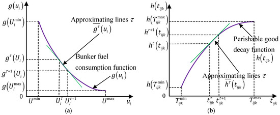
Figure 6. Piecewise linear secant approximation: (a) Bunker fuel consumption function $g\left(u_i\right)$; (b) Perishable good decay function $h\left(t_{ijk}\right)$. Source: Drawn by the authors; no copyright issues are involved.

As shown in Figure 6, increasing the number of linear secant segments $N$, allows the piecewise linear function to more closely approximate the original nonlinear function. It is worth noting that, according to the study in [77], the increase in $N$ not only improves the accuracy of approximating $g\left(u_i\right)$ and $h\left(t_{ijk}\right)$ to $\overline{g^{\tau }}\left(u_i\right)$ and $\overline{h^{\tau }}\left(t_{ijk}\right)$, respectively, but also leads to an increase in computational time. Therefore, through the aforementioned method, the nonlinear model [M1] is effectively transformed into the linear model [M2]:

Objective function:

$$\min F_2=\left\{C^{oc}m+{\displaystyle \sum _{i\in I}\left[E{b}_i+f\left(z_i\right)\right]}+{\displaystyle \sum _{i\in I}{\displaystyle \sum _{t\in T_i}{\displaystyle \sum _{h\in H_{it}}{C}_{ith}^{hc}{D}_i{y}_{ith}+C^{ic}{\displaystyle \sum _{i\in I}{t}_i{Q}_i}+{\displaystyle \sum _{i\in I}{C}_i^{lc}{t}_i^l}+{\displaystyle \sum _{i=1}^n{\displaystyle \sum _{j=1,j\ne i}^n{\displaystyle \sum _{k=1}^r{C}_k^d{R}_{ijk}\overline{h^{\tau }}\left(t_{ijk}\right)}}}}}}\right\}$$

(33)

Constraints: (2)–(8), (10)–(23), (26)–(28) and (30)

$$z_{i+1}^1=z_i^2-\overline{g^{\tau }}\left(u_i\right),\forall i\in I,i<n;\forall \tau \in \left\{1,2,\dots ,N\right\}$$

(34)

$$z_1^1=z_n^2-\overline{g^{\tau }}\left(u_n\right), \forall \tau \in \left\{1,2,\dots ,N\right\}$$

(35)

$$\overline{g^{\tau }}\left(u_i\right)\ge {\displaystyle \frac{g\left(U_i^{\tau +1}\right)-g\left(U_i^{\tau }\right)}{U_i^{\tau +1}-U_i^{\tau }}}{u}_i+{\displaystyle \frac{U_i^{\tau }g\left(U_i^{\tau +1}\right)-U_i^{\tau +1}g\left(U_i^{\tau }\right)}{U_i^{\tau }-U_i^{\tau +1}}}-M\left(1-{\alpha }_i^{\tau }\right),\forall i\in I;\tau \in \left\{1,2,\dots ,N\right\}$$

(36)

$$\overline{h^{\tau }}\left(t_{ijk}\right)\ge {\displaystyle \frac{h\left(t_{ijk}^{\tau +1}\right)-h\left(t_{ijk}^{\tau }\right)}{t_{ijk}^{\tau +1}-t_{ijk}^{\tau }}}{u}_i+{\displaystyle \frac{t_{ijk}^{\tau }h\left(t_{ijk}^{\tau +1}\right)-t_{ijk}^{\tau +1}h\left(t_{ijk}^{\tau }\right)}{t_{ijk}^{\tau }-t_{ijk}^{\tau +1}}}-M\left(1-{\beta }_{ijk}^{\tau }\right), \forall i,j\in I,i\ne j;\tau \in \left\{1,2,\dots ,N\right\};\forall k\in K$$

(37)

$$U_i^{\tau }{\alpha }_i^{\tau }\le u_i,\forall i\in I;\tau \in \left\{1,2,\dots ,N\right\}$$

(38)

$$U_i^{\tau +1}+M\left(1-{\alpha }_i^{\tau }\right)\ge u_i,\forall i\in I;\tau \in \left\{1,2,\dots ,N\right\}$$

(39)

$$t_{ijk}^{\tau }{\beta }_{ijk}^{\tau }\le t_{ijk}, \forall i,j\in I,i\ne j;\tau \in \left\{1,2,\dots ,N\right\};\forall k\in K$$

(40)

$$t_{ijk}^{\tau +1}+M\left(1-{\beta }_{ijk}^{\tau }\right)\ge t_{ijk}, \forall i,j\in I,i\ne j;\tau \in \left\{1,2,\dots ,N\right\};\forall k\in K$$

(41)

$$t_i=l_i{u}_i,\forall i\in I$$

(42)

$${\displaystyle \raisebox{1ex}{$1$}\!\left/ \!\raisebox{-1ex}{$V^{\max }$}\right.}\le u_i\le {\displaystyle \raisebox{1ex}{$1$}\!\left/ \!\raisebox{-1ex}{$V^{\min }$}\right.},\forall i\in I$$

(43)

$${\displaystyle \sum _{\tau =1}^N{\alpha }_i^{\tau }}=1,\forall i\in I$$

(44)

$${\displaystyle \sum _{\tau =1}^N{\beta }_{ijk}^{\tau }}=1,\forall i,j\in I, i\ne j;\forall k\in K$$

(45)

$${\alpha }_i^{\tau }\in \left\{0,1\right\},\forall i\in I;\forall \tau \in \left\{1,2,\dots ,N\right\}$$

(46)

$${\beta }_{ijk}^{\tau }\in \left\{0,1\right\},\forall i,j\in I, i\ne j;\forall \tau \in \left\{1,2,\dots ,N\right\};\forall k\in K$$

(47)

By replacing $h\left(t_{ijk}\right)$ with $\overline{h^{\tau }}\left(t_{ijk}\right)$ in the objective function of model [M1], the objective function of model [M2] (Equation (33)) is obtained. Regarding the constraints, Constraints (34) and (35) employ linear formulations to represent the relationship between fuel consumption and fuel inventory before and after each refueling operation. Constraint (36) estimates bunker fuel consumption through a series of piecewise linear secant approximations, while constraint (37) similarly approximates the decay of perishable goods. Constraints (38) and (39) determine the minimum and maximum values of the ship sailing speed reciprocal $u_i$ in the $\tau$-th linear segment, respectively. Similarly, Constraints (40) and (41) determine the minimum and maximum values of the total shipping time of perishable goods $t_{ijk}$ in the $\tau$-th linear segment, respectively. Constraint (42) determines the sailing time by ship sailing speed reciprocal. Constraints (43) shows a ship sailing speed reciprocal should be within specific limits. Constraint (44) indicates that only one linear function $\overline{g^{\tau }}\left(u_i\right)$ should be selected to approximate the bunker consumption function. Constraint (45) indicates that only one linear function $\overline{h^{\tau }}\left(t_{ijk}\right)$ should be selected to approximate the good decay function. Constraints (46) and (47) introduce two new binary variables. Evidently, model [M2] can be efficiently solved using off-the-shelf commercial MILP solvers such as CPLEX.

6. Numerical Experiments

This section conducts a series of numerical experiments to derive managerial insights regarding the perishable good shipping, refueling strategy, collaborative agreement formulation, etc.

6.1. Input Data Description

As shown in Figure 7, the Asia–North Europe (AEU6) liner shipping route, operated by China COSCO Shipping Group (Shanghai, China), is selected as the representative case study. Notably, Le Havre is visited twice during the rotation, while all other ports are called once. To account for the additional call to Le Havre, a virtual node is introduced in the model. Consequently, the AEU6 port rotation comprises 14 port calls (12 unique ports plus 2 calls to Le Havre), with a scheduled weekly service frequency.

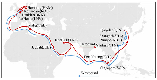
Figure 7. AEU6 route. Source: Drawn by the authors; no copyright issues are involved.

The distance between consecutive ports and fuel price at each port are presented in Table 5.

Table 5. Fuel price of port and leg distance.

Port	QIN	NBO	SHA	YTN	SGP	LHV	ROT	DKK	HAM	LHV	VEL	JED	TAT	PKL
Distance (nmi)	433	136	831	1445	8083	247	141	394	500	2150	1657	2363	3398	2673
Fuel price (USD/ton)	475	467	471	-	405	346	357	319	288	346	265	389	-	412

The name of the port is abbreviated. Source: Compiled by the authors; no copyright issues are involved.

The parameter values used in the computational experiments are drawn from data reported in the literature [5,18,20,28,34,35,53,61,67,69,78] and are summarized in Table 6.

Table 6. Numerical data.

Parameter	Value
Number of ports called: $n$	14
$\mathrm{Total} \mathrm{of} \mathrm{perishable} \mathrm{good} \mathrm{types}: \left|K\right|$	20
$\mathrm{Bunker} \mathrm{fuel} \mathrm{consumption} \mathrm{rate}: \left(\alpha ={\displaystyle \raisebox{1ex}{$F_D$}\!\left/ \!\raisebox{-1ex}{$V_D^3$}\right.}\right)$,	0.012
$\mathrm{Weekly} \mathrm{operational} \cos \mathrm{t} \mathrm{of} \mathrm{a} \mathrm{ship}: C^{oc}$(USD/week)	300,000
$\mathrm{Unit} \mathrm{container} \mathrm{inventory} \cos \mathrm{t}: C^{ic}$(USD/TEU/h)	0.5
Decay cost per unit quality loss of good type $k$$:C_k^d$ (USD/%)	$U[35;60]$
Unit penalty for late ship arrival $i$$: C_i^{lc}$ (USD/h)	$U[3000;5000]$
Container amount shipped at leg $i$$: Q_i$ (TEUs)	$U[8000;\mathrm{13,000}]$
$\mathrm{Minimum} \mathrm{fuel} \mathrm{inventory} \mathrm{at} \mathrm{the} \mathrm{beginning}: I_0$ (tons)	1000
Fixed cost of ship refueling: $E$ (USD)	1000
Ship bunker tanker maximal capacity: $W$ (tons)	5000
$\mathrm{Refueling} \mathrm{amount} \mathrm{thresholds}: W_i^1,W_i^2$ (tons)	1000, 2000
$\mathrm{Price} \mathrm{discount} \mathrm{factor} \mathrm{of} \mathrm{bunker} \mathrm{fuel}: {\lambda }_i^1,{\lambda }_i^2$ (%)	90%, 80%
Decay rate of perishable good type $k$$: {\delta }_k$ (%/h)	$U[0.0005;0.0020]$
$\mathrm{Minimum} \mathrm{ship} \mathrm{sailing} \mathrm{speed}: V^{\min }$ (knots)	15
$\mathrm{Maximum} \mathrm{ship} \mathrm{sailing} \mathrm{speed}: V^{\max }$ (knots)	25

Source: Compiled by the authors; no copyright issues are involved.

Based on data reported in the literature [5,18,20,28,34,35,53,61,67,69,78], terminal operators provides 4 ship arrival time windows per port, with each window associated with 3 start times and 3 end times. For instance, the 4 time windows offered by Qingdao port along with the corresponding start times, are summarized in Table 7.

Table 7. Time windows and corresponding start and end times provided by Qingdao Port.

Time Windows	1			2			3			4
Start time	0:00	6:00	12:00	18:00	24:00	30:00	36:00	42:00	48:00	54:00	60:00	66:00

Source: Compiled by the authors; no copyright issues are involved.

The start times $s$ of the 4 time windows at the remaining ports are determined using the formula $T{W}_{\left(i+1\right)ts}^S=T{W}_{its}^S+{\displaystyle \frac{L_i}{V_i}}$ (h). Based on actual shipping operations and ship specifications, and drawing on data from relevant studies [79,80], the estimated ship speed $V_i$ (knots) are generated using a uniform distribution $U\left[15,25\right]$. The duration of each time window at port $i$ is generated as $T{W}_{ite}^E-T{W}_{its}^S=U[24;72]$ (h). Weekly container handling volumes also vary by port size. For Large ports—Qingdao, Shanghai, Ningbo, Singapore, Rotterdam, and Port Kelang, all ranked among the world’s top 20—the weekly container handling quantity (TEUs) is generated from $U\left[500,2000\right]$. For smaller ports, weekly container handling quantity is generated from $U\left[200;1000\right]$. Each terminal provides 4 container handling rates $H{P}_{ith}$ (TEUs/h), defined as $H{P}_{ith}=H{P}_{ith}^m\pm {\Delta }_h$, where $H{P}_{ith}^m$ represents average productivity. Large ports adopt productivity levels of 50, 75, 100, and 125 TEUs/h, while smaller ports adopt 50, 60, 75, and 100 TEUs/h. And the variation ${\Delta }_h$ is generated as $U\left[0,20\right]$. The corresponding $C_{ith}^{hc}$ (USD/TEU) is calculated as $C_{ith}^{hc}=C_{ith}^m\pm {\Delta }_{hc}$, where $C_{ith}^m$ denotes the average handling cost per TEU, which is set to 475, 550, 625, and 770 USD/TEU. The deviation ${\Delta }_h$ is also generated randomly following a uniform distribution $U\left[0,50\right]$. In the numerical experiments, the route includes 14 ports of call and 20 types of perishable goods, leading to an OD flow size of 14 × 14 × 20 = 3920. Because collecting such extensive OD flow data is challenging, and two new notations are introduced: $O_k$: the origin ports of the perishable good type $k$, $D_k$: the destination ports of the perishable good type $k$. Using these, model [M2] is reformulated into the simplified model [M3] as follows:

Objective function:

$$\min F_3=\left\{C^{oc}m+{\displaystyle \sum _{i=1}^n\left[E{b}_i+f\left(z_i\right)\right]}+{\displaystyle \sum _{i\in I}{\displaystyle \sum _{t\in T_i}{\displaystyle \sum _{h\in H_{it}}{C}_{ith}^{hc}{D}_i{y}_{ith}+C^{ic}{\displaystyle \sum _{i\in I}{t}_i{Q}_i}+{\displaystyle \sum _{i\in I}{C}_i^{lc}{t}_i^l}+{\displaystyle \sum _{k=1}^r{C}_k^d{R}_{O_k{D}_{k}k}{\beta }_k^{\tau }\overline{h^{\tau }}\left(t_{O_k{D}_{k}k}\right)}}}}\right\}$$

(48)

Constraints: (2)–(8), (10), (12)–(23), (26)–(28), (30), (34)–(36), (38) and (39), (42)–(44) and (46)

$$t_{O_k{D}_{k}k}={\displaystyle \sum _{s=O_k}^{D_k}{t}_s^b}+{\displaystyle \sum _{s=O_k}^{D_k-1}{t}_s},\forall k\in K$$

(49)

$$\overline{h^{\tau }}\left(t_{O_k{D}_{k}k}\right)\ge {\displaystyle \frac{h\left(t_{O_k{D}_{k}k}^{\tau +1}\right)-h\left(t_{O_k{D}_{k}k}^{\tau }\right)}{t_{O_k{D}_{k}k}^{\tau +1}-t_{O_k{D}_{k}k}^{\tau }}}{t}_{O_k{D}_{k}k}+{\displaystyle \frac{t_k^{\tau }h\left(t_{O_k{D}_{k}k}^{\tau +1}\right)-t_k^{\tau +1}h\left(t_{O_k{D}_{k}k}^{\tau }\right)}{t_{O_k{D}_{k}k}^{\tau }-t_{O_k{D}_{k}k}^{\tau +1}}}-M\left(1-{\beta }_{O_k{D}_{k}k}^{\tau }\right),\forall k\in K,\tau \in \left\{1,2,\dots ,N\right\}$$

(50)

$$t_{O_k{D}_{k}k}^{\tau }{\beta }_{O_k{D}_{k}k}^{\tau }\le t_{O_k{D}_{k}k}, \tau \in \left\{1,2,\dots ,N\right\};\forall k\in K$$

(51)

$$t_{O_k{D}_{k}k}^{\tau +1}+M\left(1-{\beta }_{O_k{D}_{k}k}^{\tau }\right)\ge t_{O_k{D}_{k}k},\tau \in \left\{1,2,\dots ,N\right\};\forall k\in K$$

(52)

$${\displaystyle \sum _{\tau =1}^N{\beta }_{O_k{D}_{k}k}^{\tau }}=1,\forall k\in K$$

(53)

$${\beta }_{O_k{D}_{k}k}^{\tau }\in \left\{0,1\right\},\forall k\in K,\forall \tau \in \left\{1,2,\dots ,N\right\}$$

(54)

According to the model [M3], the OD flow parameter data decreased from 3920 to 20 after $R_{ijk}$ is replaced by $R_{O_k{D}_{k}k}$ in the volume of the perishable good type $k$. During the data simulation, the loading of refrigerated containers must satisfy the power outlet requirements of each ship; hence, the data are configured subject to constraints (26)–(28). Assuming that each ship is equipped with 5000 power outlets, the average number of outlet turnovers across the round trip is uniformly distributed as $U\left[1,2\right]$ (times), which corresponds to a freezer capacity equivalent to $U\left[5000,\mathrm{10,000}\right]$ TEUs. Accordingly, when the number $R_{O_k{D}_{k}k}$ of perishable good type $k$ is randomly generated from a uniform distribution $U\left[1,n-1\right]$ (TEUs), the origin port $O_k$ is drawn from $U\left[1,n-1\right]$, and the destination port $D_k$ from $U\left[O_k+1,n\right]$. This procedure yields the distribution of refrigerated containers across all voyage legs.

6.2. Solution Methodology Evaluation and Complexity Analysis

6.2.1. Solution Methodology Evaluation

To evaluate the impact of the number of linear segments on computational accuracy and solving time, a series of tests are conducted to determine the appropriate number of segments. Existing studies typically use integer segment quantities [79,80]. Based on relevant evaluation methods, six evaluation scenarios are constructed by changing the number of linear segments in the linear secant approximation, with the segment number uniformly increasing from 10 to 60. To facilitate calculation and comparison, the median values of the uniform distribution parameters are selected for evaluation. MATLAB 2016a is used to simulate the piecewise linear approximation function. The model [M1] is solved using Lingo 11, with a solving time set to 1h and a global optimal accuracy requirement. Model [M2] is solved using ILOG CPLEX 12.6.2 with default solver parameters, and the solution gap for all six instances are maintained below 0.01%, achieving satisfactory solution accuracy. All experiments are conducted on a computer equipped with a 12th Gen Intel^® Core™ i5-12500H (2.50 GHz) processor (Intel Corporation, Santa Clara, CA, USA) and 16 GB RAM. Table 8 presents the total service cost and calculation time for different numbers of linear segments.

Table 8. Total liner route service cost and calculation time for different number of linear segments.

Instance	Number of Linear Segments	Total Liner Route Service Cost by Model [M2] $\mathit{L}\mathit{B}$ (103 USD)	Total Liner Route Service Cost by Model [M1] $\mathit{L}\mathit{C}$ (103 USD)	GAP (%)	CPU Time (s)
1	10	17,224.36	17,227.35	−0.0174	0.56
2	20	17,226.09		−0.0073	0.81
3	30	17,227.18		−0.0010	1.54
4	40	17,227.52		0.0010	2.89
5	50	17,227.53		0.0010	4.30
6	60	17,227.54		0.0011	5.92

Source: Compiled by the authors; no copyright issues are involved.

As shown in Table 8, with an increasing number of linear segments, the total service cost approaches the optimal value, but the computational time increases. In addition, the GAP show that when the number of linear segments exceeds 40, model [M2] obtains more accurate solutions than model [M1] within a shorter computation time. Where $GAP={\displaystyle \frac{LB-LC}{LC}}\times 100\%$, GAP > 0 indicates that the solution obtained by model [M2] is better than that of model [M1], whereas GAP < 0 indicates the opposite. To strike a balance between computational error and solving time, 40 linear segments are selected in this study.

6.2.2. Complexity Analysis

The MILP model presented in this study includes both binary and continuous variables. The computational complexity of such models, in theory, grows exponentially with respect to the number of binary variables, represented as $O\left(2^{\eta }\cdot poly\left(\xi \right)\right)$, where $\eta$ is the number of binary variables, and $\xi$ is the number of continuous variables. Each binary variable corresponds to a branch in the search tree, while each node in the tree requires solving a continuous linear programming (LP) problem. This exponential growth is typical for MILP models due to the combinatorial nature of binary decisions. In practice, however, modern solvers such as CPLEX leverage advanced optimization techniques, including branch-and-bound, cutting planes, and heuristic strategies. These methods significantly reduce the effective search space. As a result, the computational burden is mitigated, and the model can be solved in a reasonable amount of time for practical problem sizes.

For real-world long-haul shipping routes, the number of ports typically ranges from 10 to 20, reflecting operational realities where shipping companies manage a limited number of ports along each route. Accordingly, the impact of port count on computation time is expected to be moderate. In the AEU6 instance considered in this study, the model includes 1934 binary variables and 1569 continuous variables, a size that is well within the capacity of modern solvers. The complexity of the problem, including the number of ports, TWs and container handling rates, as well as refueling options, affects CPU time. However, given that the model is designed with realistic operational constraints, the computational time does not grow prohibitively as the number of ports.

6.3. Results Analysis

In this section, the experimental results are analyzed from three aspects, including: (1) ship scheduling and refueling strategy; (2) comparative analysis with other models; (3) sensitivity analysis of model [M3].

6.3.1. Results Pertaining to the AEU6 Route

Based on the collected data, 1000 scenarios are generated following the specified numerical rules. Each scenario can be solved efficiently, requiring less than 10 s of computation, with the solution gap controlled within 0.01%. The numerical analysis is performed using CPLEX implemented in GAMS 23.9, yielding the optimal round-trip ship schedule and corresponding refueling strategy, as presented in Table 9.

Table 9. Ship schedule and refueling results for the AEU6 route.

Port	Leg	Arrival Time (h)	Departure Time (h)	Bunker Consumption (Tons)	Fuel Inventory (Tons)	Refueling Amount (Tons)
QIN	QIN → NBO	0	30	131	1000	-
NBO	NBO → SHA	47	74	42	869	-
SHA	SHA → YTN	80	106	253	827	500
YTN	YTN → SGP	140	160	433	1074	-
SGP	SGP → LHV	220	248	2386	641	3325
LHV	LHV → ROT	582	606	75	1580	-
ROT	ROT → DKK	617	650	43	1505	-
DKK	DKK → HAM	656	670	122	1462	-
HAM	HAM → LHV	685	700	154	1340	-
LHV	LHV → VEL	720	735	665	1186	-
VEL	VEL → JED	822	841	510	521	3565
JED	JED → TAT	908	933	730	3576	-
TAT	TAT → PKL	1028	1063	1055	2846	-
PKL	PKL → QIN	1199	1233	791	1791	-
QIN	-	1344	1374	-	-	-

Source: Compiled by the authors; no copyright issues are involved.

As shown in Table 9, the total time for a complete round-trip voyage is 1344 h (8 weeks), with eight ships allocated to the service. Refueling occurs at three ports: Shanghai, Singapore, and Malta. The refueling strategy is guided by port-specific fuel prices and fuel inventory levels, resulting in the majority of refueling taking place at ports with relatively lower bunker costs, while the refueling amounts vary across ports. This numerical experiment highlights the impact of refueling strategies on overall operations, demonstrating how port fuel prices, container handling rates, and the selection of ship arrival time windows jointly shape the ship schedule.

6.3.2. Comparative Analysis

The effectiveness and practical applicability of the proposed model are evaluated through a comparative analysis of three alternative approaches to ship scheduling and refueling strategy, including the following:

• Model [M3]: Ship scheduling and refueling under collaborative agreements, accounting for the shipping of perishable goods and port fuel price differences, including amount-based discounts.
• Model [M4]: Ship scheduling and refueling considering port fuel price differences and discounts. Multiple handling rates are available, while ship arrival time windows are fixed.
• Model [M5]: Ship scheduling and refueling under collaborative agreements, considering port fuel price differences and discounts, but excluding the shipping of perishable goods.

The performance of models [M3], [M4], and [M5] is compared across several key indicators: (1) total liner route service cost—TRC; (2) mean sailing speed—MS; (3) total handling cost—THC; (4) total number of ships deployed—Q; (5) total late arrival penalty—TLC; (6) total bunker cost—TBC; (7) total refueling amount—TRA; (8) total good decay cost—TAC and (9) refueling amount at port. Table 10 summarizes the average values of these indicators across 1000 simulated scenarios for the different models.

Table 10. Comparison of indicators for different models.

Model	TRC (103 USD)	MS (Knots)	THC (103 USD)	Q (Vessels)	TLC (103 USD)	TBC (103 USD)	TRA (Tons)	TAC (103 USD)	Refueling Amount at Port (Tons)
									QIN	SHA	SGP	DKK	HAM	VEL
[M3]	17,204	24.46	5887	8.00	255	2273	7390	1157	-	500	3325	-	-	3565
[M4]	18,023	23.79	6363	8.00	559	2192	7105	1122	-	564	2605	-	563	3373
[M5]	15,754	24.45	5550	8.00	254	2307	7375	-	851	-	2222	616	-	3686

Source: Compiled by the authors; no copyright issues are involved.

As shown in Table 10, compared with model [M4], model [M3] achieves a lower total route service cost, as well as reduced container handling and late arrival penalty costs. Specifically, the total route service cost and handling cost decrease by 4.5% and 7.5%, respectively. This improved performance is primarily attributable to the consideration of port fuel price differences and discount factors, which allow the liner company to select refueling ports with lower bunker costs and optimize refueling amounts to maximize discounts. Furthermore, the inclusion of collaborative agreements with terminal operators provides multiple options for arrival time windows and port handling rates, significantly enhancing scheduling flexibility. This flexibility enables ships to adjust arrival and departure times according to operational conditions, minimizing delays and improving overall efficiency. Similarly, access to multiple handling rates allows for optimization of both cost and port time. Together, these options facilitate a global optimization of ship sailing speeds, refueling strategies, scheduling times, and handling rates, ultimately reducing overall operational costs. While higher sailing speeds increase bunker consumption, the optimized refueling strategy effectively offsets this additional expense. It is worth noting that, under model [M3], lower efficiency in some port handling rates can lead to an increase in the total cost associated with the decay of perishable goods. However, this impact can be mitigated, as shipping companies can negotiate with terminal operators to adjust time windows, making them more conducive to the handling of perishable goods. Compared with model [M5], which excludes perishable goods, model [M3] accounts for their shipping, resulting in higher average sailing speeds and improved port handling efficiency. Although the mean sailing speed across all voyage legs shows minimal variation, significant differences exist at the individual leg level, affecting refueling port choices, refueling amounts, and associated costs. This underscores the practical significance of incorporating perishable goods and collaborative agreements into ship scheduling and refueling strategies.

6.3.3. Sensitivity Analysis

In actual operation, changes in the duration of the TWs, bunker fuel price, fuel consumption rate, and fuel tank capacity can significantly influence schedule design and refueling strategy. To examine these impacts, a sensitivity analysis is conducted.

• Duration of the TWs

Ten calculation scenarios are generated by varying the duration of the TWs from (24–29) to (69–72). Figure 8 presents the corresponding average performance indicators under these TW durations, along with the associated optimal refueling strategies.

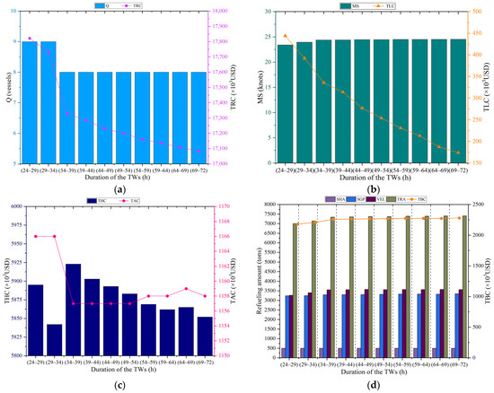
Figure 8. Computational results at different duration of the TWs scenarios for AEU6 service: (a) Total cost and number of ships; (b) Mean speed and total late arrival penalty; (c) Total handling cost and total good decay cost; (d) Refueling strategy. Source: Drawn by the authors; no copyright issues are involved.

As shown in Figure 8, extending the duration of the TWs decreases total route service cost, handling cost, late-arrival penalties, and the decay cost of perishable goods. Longer time windows provide greater operational flexibility, enabling shipping companies to select lower handling rates, thereby reducing handling cost. However, this flexibility also results in marginal increases in sailing speed, total bunker cost, and total refueling amount. To offset the longer port stays while maintaining the same fleet size, ships accelerate sailing speed, which slightly raises fuel consumption and refueling requirements. In addition, reductions in total sailing and handling time shorten the overall turnaround time, enabling the service to operate with fewer vessels while maintaining service frequency.

2.

Fuel Price

The next analysis examines the impact of bunker fuel price. Ten scenarios are generated, wherein fuel price decreases by 30%, 20%, and 10%, and increases by 10%, 20%, 30%, 40%, 50%, and 60%. Figure 9 summarizes the average performance indicators and the corresponding optimal refueling strategies for each scenario.

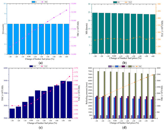
Figure 9. Computational results at different bunker fuel price scenarios for AEU6 service: (a) Total cost and number of ships; (b) Mean speed and total late arrival penalty; (c) Total handling cost and total good decay cost; (d) Refueling strategy. Source: Drawn by the authors; no copyright issues are involved.

As the results indicate, bunker cost increases sharply as fuel prices rise, leading to a reduction in ship sailing speed and a corresponding increase in total service cost. The decay cost of perishable goods and handling cost also show moderate increases. For example, when bunker fuel prices rise by 60%, the total handling cost increases by 109 × 10³ USD compared with the scenario in which fuel prices decrease by 30%. This outcome reflects the specific requirements of perishable goods, which necessitate higher sailing speeds and more efficient port handling. When fuel prices escalate, shipping companies balance bunker and handling costs by reducing sailing speed, adjusting refueling decisions, and shortening port stay durations.

3.

Bunker Fuel Consumption Rate

Next, ten scenarios are developed to examine the effect of the bunker fuel consumption rate, with values ranging from 0.0008 to 0.0017. Figure 10 presents the resulting performance indicators and the corresponding optimal refueling strategies for each consumption rate scenario.

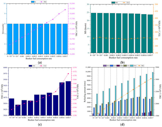
Figure 10. Computational results at different bunker fuel consumption rate scenarios for AEU6 service: (a) Total cost and number of ships; (b) Mean speed and total late arrival penalty; (c) Total handling cost and total good decay cost; (d) Refueling strategy. Source: Drawn by the authors; no copyright issues are involved.

An increase in the bunker fuel consumption rate produces trends similar to those observed in the fuel price scenarios. Higher consumption rates lead to sharp increases in total service cost, handling cost, bunker cost, perishable goods decay cost, and total refueling amount, while average sailing speed declines notably. In contrast, fleet size and total late arrival penalties remain largely unaffected. Refueling strategies adjust in response to higher consumption levels. As the consumption rate increases, the ship draws substantially more fuel at Singapore and Malta, whereas refueling amounts at Shanghai remain almost unchanged. At the highest consumption rates (0.0016 and 0.0017), Dunkirk becomes an additional refueling port, absorbing part of the fuel previously loaded at Singapore and Malta. This shift reflects a stronger preference for ports offering comparatively lower fuel prices when consumption is high. Overall, significant variations in bunker fuel consumption rate and price necessitate re-optimization of ship scheduling and refueling strategies.

4.

Bunker Fuel Capacity

Finally, five bunker fuel capacity scenarios ranging from 3000 to 7000 tons are analyzed. Figure 11 presents the corresponding performance indicators and the optimal refueling strategies for each capacity level.

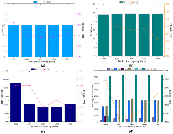
Figure 11. Computational results at different bunker fuel capacity scenarios for AEU6 service: (a) Total cost and number of ships; (b) Mean speed and total late arrival penalty; (c) Total handling cost and total good decay cost; (d) Refueling strategy.Source: Drawn by the authors; no copyright issues are involved.

The results show that bunker fuel capacity has a direct influence on total service cost, handling cost, bunker cost, total refueling amount, and average sailing speed. The computational analysis suggests that capacities of 5000 and 6000 tons offer the most balanced performance for scheduling and refueling decisions. When fuel capacity is too low, ships must refuel more frequently, which increases total refueling cost and reduces sailing speed. Longer port stays also heighten the risk of perishable goods decay, compelling operators to use higher port handling rates. In contrast, excessively large fuel tanks may reduce available cargo space and potentially diminish freight revenue. Overall, the findings indicate that bunker fuel capacity plays a critical role in operational performance. Selecting an appropriate capacity is essential for achieving an optimal balance between ship scheduling efficiency and refueling strategies.

6.4. Discussion

Based on the preceding analysis, several key research findings and managerial insights can be highlighted:

• For container liner shipping services carrying significant volumes of perishable goods, scheduling and refueling decisions should consider not only fluctuations in shipping demand and bunker fuel prices but also the underlying demand structure, particularly perishable goods and its decay characteristics. To optimize schedules, minimize total service costs, and ensure sufficient fuel supply, differences in fuel prices must be incorporated into the scheduling and refueling strategy.
• The duration of TWs strongly influences the selection of handling rates and port time. Longer TWs provide greater operational flexibility, allowing for optimized handling rates that reduce both container handling costs and perishable goods decay, thereby lowering overall service costs. Liner shipping companies are encouraged to establish robust collaborative agreements with terminal operators, formalizing mutually beneficial arrangements that enhance operational efficiency and maximize revenue.
• The total decay cost of perishable goods and overall service costs are positively correlated with bunker fuel prices. Higher fuel prices typically lead ships to reduce sailing speed, extending cargo transit times and increasing container handling, inventory costs, and late arrival penalties. By integrating optimized schedule planning with strategic refueling, liner operators can mitigate the escalation of service costs under high fuel prices.
• Ship bunker fuel consumption rates have a significant impact on scheduling and refueling decisions. On routes with a high proportion of perishable goods, operators should prioritize modern, fuel-efficient ships capable of maintaining higher speeds at lower cost. To maintain schedule reliability and profitability, companies should consider timely retrofitting of existing ships or reserving upgrade-ready spaces during new ship construction.
• Bunker tank capacity affects eligibility for fuel purchase discounts, creating a cascading effect on operational decisions. Ship designs should therefore rationally account for bunker fuel capacity, considering route characteristics, operational patterns, and vessel specifications to optimize both fuel procurement and voyage efficiency.
• Shipping companies can further reduce cost uncertainty by proactively planning fuel procurement and establishing fuel supply agreements with ports. This strategy is particularly critical for long-haul routes with substantial perishable goods, enabling stable and cost-effective fuel supply, supporting higher sailing speeds, and minimizing product decay.
• The methods proposed in this study enable shipping companies to determine optimal port time windows and container handling rates. Terminal operators, as partners, can then allocate berths and port equipment in advance according to these schedules. This collaborative approach fosters operational stability, ensures orderly execution of schedules, and creates mutual benefits for both shipping companies and terminal operators.

7. Conclusions and Future Research Extensions

This study develops an effective ship scheduling and refueling strategy for perishable goods shipping, accounting for the characteristics and decay dynamics of reefers as well as the variations and fluctuations of bunker fuel prices across different ports. A MINLP model is formulated to minimize total shipping service cost, and a piecewise linear secant approximation method is employed to linearize nonlinear functions. Application of the proposed model and solution methodology to the AEU6 route case study validates both its effectiveness and practical relevance.

The study provides valuable contributions to existing research and plays an important role in advancing the high-quality development of the shipping industry. Nonetheless, several limitations should be acknowledged. The optimization results are derived under fixed parameters and expected operating conditions, and the analysis is based on a number of simplifying assumptions. In addition, the study examines a single route operated by a homogeneous fleet. Future work could extend the proposed framework to multi-route networks with heterogeneous vessels. Given the uncertainties inherent in shipping markets and navigation conditions, developing robust or stochastic scheduling and refueling strategies represents a promising direction. Another important avenue for research is the exploration of alternative decay functions for perishable goods and the incorporation of uncertainty in decay prediction.

References

- Øvstebø, B.O.; Hvattum, L.M.; Fagerholt, K. Routing and scheduling of RoRo ships with stowage constraints. Transp. Res. Part C Emerg. Technol. 2011, 19, 1225–1242. [Google Scholar] [CrossRef]
- CTS Team, Container Trades Statistics Ltd. (CTS). 2024 Annual Overview: Global Volumes Reach New Heights. 2025. Available online: https://containerstatistics.com/annual-2024-press-release/?utm_source=chatgpt.com (accessed on 8 August 2025).
- Accenture Cargo. Global Reefer Market Outlook. 2024. Available online: https://tpm.joc.com/content/dam/events/tpm/tpm24-presentations/MichelLooten_TPM%20Cold%20Chain_final.pdf?utm_source=chatgpt.com (accessed on 8 July 2025).
- Mark Buzinkay, Reefer Service—Market Outlook 2024. 2024. Available online: https://www.identecsolutions.com/news/reefer-service-market-outlook-2024?utm_source=chatgpt.com (accessed on 8 September 2025).
- Dulebenets, M.A.; Ozguven, E.E. Vessel scheduling in liner shipping: Modeling transport of perishable assets. Int. J. Prod. Econ. 2017, 184, 141–156. [Google Scholar] [CrossRef]
- Rong, A.; Akkerman, R.; Grunow, M. An optimization approach for managing fresh food quality throughout the supply chain. Int. J. Prod. Econ. 2011, 131, 421–429. [Google Scholar] [CrossRef]
- Wang, X.; Li, D. A dynamic product quality evaluation based pricing model for perishable food supply chains. Omega 2012, 40, 906–917. [Google Scholar] [CrossRef]
- Grunow, M.; Piramuthu, S. RFID in highly perishable food supply chains—Remaining shelf life to supplant expiry date? Int. J. Prod. Econ. 2013, 146, 717–727. [Google Scholar] [CrossRef]
- Aung, M.M.; Chang, Y.S. Temperature management for the quality assurance of a perishable food supply chain. Food Control. 2014, 40, 198–207. [Google Scholar] [CrossRef]
- Haass, R.; Dittmer, P.; Veigt, M.; Lütjen, M. Reducing food losses and carbon emission by using autonomous control—A simulation study of the intelligent container. Int. J. Prod. Econ. 2015, 164, 400–408. [Google Scholar] [CrossRef]
- Forbes, A. The geography of transport systems. Aust. J. Marit. Ocean. Aff. 2014, 6, 113–114. [Google Scholar] [CrossRef]
- Li, Z.; Yu, X.; Shang, J.; Chen, K.; Xin, X.; Zhang, W.; Yu, S. Container Liner Shipping System Design Considering Methanol-Powered Vessels. J. Mar. Sci. Eng. 2025, 13, 709. [Google Scholar] [CrossRef]
- Zhou, J.; Zhao, Y.; Yan, X.; Wang, M. Strategy and Impact of Liner Shipping Schedule Recovery under ECA Regulation and Disruptive Events. J. Mar. Sci. Eng. 2024, 12, 1405. [Google Scholar] [CrossRef]
- Duan, W.; Li, Z.; Zhou, Y.; Deng, Z. A Novel Technical Framework for the Evaluation of Node Significance and Edge Connectivity in Global Shipping Network. J. Mar. Sci. Eng. 2024, 12, 1239. [Google Scholar] [CrossRef]
- Li, D.-C.; Yang, H.-L. Designing scheduled route for river liner shipping services with empty container repositioning. Expert Syst. Appl. 2024, 247, 123246. [Google Scholar] [CrossRef]
- Amorim, P.; Belo-Filho, M.A.F.; Toledo, F.M.B.; Almeder, C.; Almada-Lobo, B. Lot sizing versus batching in the production and distribution planning of perishable goods. Int. J. Prod. Econ. 2013, 146, 208–218. [Google Scholar] [CrossRef]
- Notteboom, T.E. The Time Factor in Liner Shipping Services. Marit. Econ. Logist. 2006, 8, 19–39. [Google Scholar] [CrossRef]
- Qiang, M.; Shuaian, W.; Andersson, H.; Thun, K. Containership Routing and Scheduling in Liner Shipping: Overview and Future Research Directions. Transp. Sci. 2014, 48, 265–280. [Google Scholar] [CrossRef]
- Notteboom, T.E.; Vernimmen, B. The effect of high fuel costs on liner service configuration in container shipping. J. Transp. Geogr. 2009, 17, 325–337. [Google Scholar] [CrossRef]
- Ronen, D. The effect of oil price on containership speed and fleet size. J. Oper. Res. Soc. 2011, 62, 211–216. [Google Scholar] [CrossRef]
- Fagerholt, K.; Laporte, G.; Norstad, I. Reducing fuel emissions by optimizing speed on shipping routes. J. Oper. Res. Soc. 2010, 61, 523–529. [Google Scholar] [CrossRef]
- Kontovas, C.A. The Green Ship Routing and Scheduling Problem (GSRSP): A conceptual approach. Transp. Res. Part D Transp. Environ. 2014, 31, 61–69. [Google Scholar] [CrossRef]
- Psaraftis, H.N.; Kontovas, C.A. Ship speed optimization: Concepts, models and combined speed-routing scenarios. Transp. Res. Part C Emerg. Technol. 2014, 44, 52–69. [Google Scholar] [CrossRef]
- Fagerholt, K.; Gausel, N.T.; Rakke, J.G.; Psaraftis, H.N. Maritime routing and speed optimization with emission control areas. Transp. Res. Part C Emerg. Technol. 2015, 52, 57–73. [Google Scholar] [CrossRef]
- Fagerholt, K.; Psaraftis, H.N. On two speed optimization problems for ships that sail in and out of emission control areas. Transp. Res. Part D Transp. Environ. 2015, 39, 56–64. [Google Scholar] [CrossRef]
- Mansouri, S.A.; Lee, H.; Aluko, O. Multi-objective decision support to enhance environmental sustainability in maritime shipping: A review and future directions. Transp. Res. Part E Logist. Transp. Rev. 2015, 78, 3–18. [Google Scholar] [CrossRef]
- Song, D.-P.; Li, D.; Drake, P. Multi-objective optimization for planning liner shipping service with uncertain port times. Transp. Res. Part E Logist. Transp. Rev. 2015, 84, 1–22. [Google Scholar] [CrossRef]
- Dulebenets, M.A. A comprehensive multi-objective optimization model for the vessel scheduling problem in liner shipping. Int. J. Prod. Econ. 2018, 196, 293–318. [Google Scholar] [CrossRef]
- Zhang, M.; Zeng, X.; Tan, Z. Joint decision of green technology adoption and sailing pattern for a coastal ship under ECAs. Transp. Policy 2024, 146, 102–113. [Google Scholar] [CrossRef]
- Sun, Y.; Zheng, J.; Cui, D.; Liu, H. Carbon emission reduction by forming liner alliances under maritime emission trading system. Transp. Res. Part D Transp. Environ. 2025, 144, 104771. [Google Scholar] [CrossRef]
- Vernimmen, B.; Dullaert, W.; Engelen, S. Schedule Unreliability in Liner Shipping: Origins and Consequences for the Hinterland Supply Chain. Marit. Econ. Logist. 2007, 9, 193–213. [Google Scholar] [CrossRef]
- Chuang, T.-N.; Lin, C.-T.; Kung, J.-Y.; Lin, M.-D. Planning the route of container ships: A fuzzy genetic approach. Expert Syst. Appl. 2010, 37, 2948–2956. [Google Scholar] [CrossRef]
- Qi, X.; Song, D.-P. Minimizing fuel emissions by optimizing vessel schedules in liner shipping with uncertain port times. Transp. Res. Part E Logist. Transp. Rev. 2012, 48, 863–880. [Google Scholar] [CrossRef]
- Wang, S.; Meng, Q. Robust schedule design for liner shipping services. Transp. Res. Part E Logist. Transp. Rev. 2012, 48, 1093–1106. [Google Scholar] [CrossRef]
- Wang, S.; Meng, Q. Liner ship route schedule design with sea contingency time and port time uncertainty. Transp. Res. Part B Methodol. 2012, 46, 615–633. [Google Scholar] [CrossRef]
- Wang, S. Optimal sequence of container ships in a string. Eur. J. Oper. Res. 2015, 246, 850–857. [Google Scholar] [CrossRef]
- Li, M.; Xie, C.; Li, X.; Karoonsoontawong, A.; Ge, Y.-E. Robust liner ship routing and scheduling schemes under uncertain weather and ocean conditions. Transp. Res. Part C Emerg. Technol. 2022, 137, 103593. [Google Scholar] [CrossRef]
- Zhang, X.; Li, R.; Wang, C.; Xue, B.; Guo, W. Robust optimization for a class of ship traffic scheduling problem with uncertain arrival and departure times. Eng. Appl. Artif. Intell. 2024, 133, 108257. [Google Scholar] [CrossRef]
- Xia, Z.; Guo, Z.; Wang, W.; Jiang, Y. Joint optimization of ship scheduling and speed reduction: A new strategy considering high transport efficiency and low carbon of ships in port. Ocean Eng. 2021, 233, 109224. [Google Scholar] [CrossRef]
- Zhen, L.; Jiang, M.; Wang, S.; Wu, J. Ship fleet scheduling and deployment optimization considering carbon and sulfur emissions. Eur. J. Oper. Res. 2025, 329, 653–668. [Google Scholar] [CrossRef]
- Ganjian, M.; Bagherian Farahabadi, H.; Rezaei Firuzjaei, M. Voyage scheduling and energy management co-optimization in hydrogen-powered ships. Int. J. Hydrogen Energy 2024, 86, 788–799. [Google Scholar] [CrossRef]
- Brouer, B.D.; Dirksen, J.; Pisinger, D.; Plum, C.E.M.; Vaaben, B. The Vessel Schedule Recovery Problem (VSRP)—A MIP model for handling disruptions in liner shipping. Eur. J. Oper. Res. 2013, 224, 362–374. [Google Scholar] [CrossRef]
- Chen, L.; Xiangtong, Q.; Chung-Yee, L. Disruption Recovery for a Vessel in Liner Shipping. Transp. Sci. 2015, 49, 900–921. [Google Scholar] [CrossRef]
- Li, C.; Qi, X.; Song, D. Real-time schedule recovery in liner shipping service with regular uncertainties and disruption events. Transp. Res. Part B Methodol. 2016, 93, 762–788. [Google Scholar] [CrossRef]
- Abioye, O.F.; Dulebenets, M.A.; Pasha, J.; Kavoosi, M. A Vessel Schedule Recovery Problem at the Liner Shipping Route with Emission Control Areas. Energies 2019, 12, 2380. [Google Scholar] [CrossRef]
- Elmi, Z.; Li, B.; Liang, B.; Lau, Y.-Y.; Borowska-Stefańska, M.; Wiśniewski, S.; Dulebenets, M.A. An epsilon-constraint-based exact multi-objective optimization approach for the ship schedule recovery problem in liner shipping. Comput. Ind. Eng. 2023, 183, 109472. [Google Scholar] [CrossRef]
- Elmi, Z.; Li, B.; Fathollahi-Fard, A.M.; Tian, G.; Borowska-Stefańska, M.; Wiśniewski, S.; Dulebenets, M.A. Ship schedule recovery with voluntary speed reduction zones and emission control areas. Transp. Res. Part D Transp. Environ. 2023, 125, 103957. [Google Scholar] [CrossRef]
- Zheng, J.; Mao, C.; Li, Y.; Liu, Y.; Wang, Y. Dynamic vessel schedule recovery strategy of liner shipping with uncertainties: An event-triggered model predictive control solution. Comput. Ind. Eng. 2024, 193, 110340. [Google Scholar] [CrossRef]
- Zhao, S.; Yang, H.; Zheng, J.; Li, D. A two-step approach for deploying heterogeneous vessels and designing reliable schedule in liner shipping services. Transp. Res. Part E Logist. Transp. Rev. 2024, 182, 103416. [Google Scholar] [CrossRef]
- Wang, S.; Alharbi, A.; Davy, P. Liner ship route schedule design with port time windows. Transp. Res. Part C Emerg. Technol. 2014, 41, 1–17. [Google Scholar] [CrossRef]
- Alharbi, A.; Wang, S.; Davy, P. Schedule design for sustainable container supply chain networks with port time windows. Adv. Eng. Inform. 2015, 29, 322–331. [Google Scholar] [CrossRef]
- Liu, Z.; Wang, S.; Du, Y.; Wang, H.J.T.J. Supply chain cost minimization by collaboration between liner shipping companies and port operators. Transp. J. 2016, 55, 296–314. [Google Scholar] [CrossRef]
- Dulebenets, M.A. Minimizing the Total Liner Shipping Route Service Costs via Application of an Efficient Collaborative Agreement. IEEE Trans. Intell. Transp. Syst. 2019, 20, 123–136. [Google Scholar] [CrossRef]
- Dulebenets, M.A. Multi-objective collaborative agreements amongst shipping lines and marine terminal operators for sustainable and environmental-friendly ship schedule design. J. Clean. Prod. 2022, 342, 130897. [Google Scholar] [CrossRef]
- Guerriero, F.; Macrina, G.; Mosca, V.; Scalzo, E. The vehicle routing problem and integrated challenges in the perishable product supply chain. Comput. Ind. Eng. 2025, 209, 111428. [Google Scholar] [CrossRef]
- Ahemad, F.; Kannan, D.; Khan, A.Z.; Gupta, P.; Mehlawat, M.K.; Aggarwal, U. Optimizing sustainable transportation planning for perishable goods: A two-stage fuzzy approach with route selection. Res. Transp. Bus. Manag. 2026, 64, 101537. [Google Scholar] [CrossRef]
- Hasiloglu-Ciftciler, M.; Kaya, O. Dynamic inventory control and pricing strategies for perishable products considering both profit and waste. Comput. Oper. Res. 2025, 181, 107103. [Google Scholar] [CrossRef]
- Wang, S.; Meng, Q.; Liu, Z. Containership scheduling with transit-time-sensitive container shipment demand. Transp. Res. Part B Methodol. 2013, 54, 68–83. [Google Scholar] [CrossRef]
- Wang, S.; Meng, Q.; Lee, C.-Y. Liner container assignment model with transit-time-sensitive container shipment demand and its applications. Transp. Res. Part B Methodol. 2016, 90, 135–155. [Google Scholar] [CrossRef]
- Kim, H.-J.; Chang, Y.-T.; Kim, K.-T.; Kim, H.-J. An epsilon-optimal algorithm considering greenhouse gas emissions for the management of a ship’s bunker fuel. Transp. Res. Part D Transp. Environ. 2012, 17, 97–103. [Google Scholar] [CrossRef]
- Yao, Z.; Ng, S.H.; Lee, L.H. A study on bunker fuel management for the shipping liner services. Comput. Oper. Res. 2012, 39, 1160–1172. [Google Scholar] [CrossRef]
- Kim, H.J. A Lagrangian heuristic for determining the speed and bunkering port of a ship. J. Oper. Res. Soc. 2014, 65, 747–754. [Google Scholar] [CrossRef]
- Sheng, X.; Lee, L.; Chew, E. Dynamic determination of vessel speed and selection of bunkering ports for liner shipping under stochastic environment. OR Spectr. 2014, 36, 455–480. [Google Scholar] [CrossRef]
- Sheng, X.; Chew, E.P.; Lee, L.H. (s,S) policy model for liner shipping refueling and sailing speed optimization problem. Transp. Res. Part E Logist. Transp. Rev. 2015, 76, 76–92. [Google Scholar] [CrossRef]
- Meng, Q.; Wang, S.; Lee, C.-Y. A tailored branch-and-price approach for a joint tramp ship routing and bunkering problem. Transp. Res. Part B Methodol. 2015, 72, 1–19. [Google Scholar] [CrossRef]
- Wang, S.; Meng, Q. Robust bunker management for liner shipping networks. Eur. J. Oper. Res. 2015, 243, 789–797. [Google Scholar] [CrossRef]
- De, A.; Choudhary, A.; Turkay, M.; Tiwari, M.K. Bunkering policies for a fuel bunker management problem for liner shipping networks. Eur. J. Oper. Res. 2019, 289, 927–939. [Google Scholar] [CrossRef]
- Aydin, N.; Lee, H.; Mansouri, S.A. Speed optimization and bunkering in liner shipping in the presence of uncertain service times and time windows at ports. Eur. J. Oper. Res. 2017, 259, 143–154. [Google Scholar] [CrossRef]
- Wang, C.; Chen, J. Strategies of refueling, sailing speed and ship deployment of containerships in the low-carbon background. Comput. Ind. Eng. 2017, 114, 142–150. [Google Scholar] [CrossRef]
- Wang, S.; Gao, S.; Tan, T.; Yang, W. Bunker fuel cost and freight revenue optimization for a single liner shipping service. Comput. Oper. Res. 2019, 111, 67–83. [Google Scholar] [CrossRef]
- Wang, C.; Liu, X.; Zhou, Y.; Qian, J. Optimization of speed and refueling strategy for liner shipping companies considering refueling at OPL. Reg. Stud. Mar. Sci. 2025, 89, 104355. [Google Scholar] [CrossRef]
- Du, J.; Wu, P. Stochastic dynamic programming model for liner international scheduling optimization under ECA policies. Mar. Pollut. Bull. 2026, 222, 118766. [Google Scholar] [CrossRef]
- Wu, Y.; Guo, H.; Qi, J.; Wang, S.; Zhen, L. Ship refueling optimization for dual-fuel ships considering carbon intensity indicator rating limit and uncertain fuel prices. Multimodal Transp. 2024, 3, 100138. [Google Scholar] [CrossRef]
- Gao, T.; Tian, J.; Liu, C.; Huang, C.; Wu, H.; Yuan, Z. A model for speed and fuel refueling strategy of methanol dual-fuel liners with emission control areas. Transp. Policy 2025, 161, 1–16. [Google Scholar] [CrossRef]
- Jiang, L.; Kronbak, J.; Christensen, L.P. The costs and benefits of sulphur reduction measures: Sulphur scrubbers versus marine gas oil. Transp. Res. Part D Transp. Environ. 2014, 28, 19–27. [Google Scholar] [CrossRef]
- Wang, S.; Meng, Q.; Liu, Z. Bunker consumption optimization methods in shipping: A critical review and extensions. Transp. Res. Part E Logist. Transp. Rev. 2013, 53, 49–62. [Google Scholar] [CrossRef]
- Vielma, J.P.; Ahmed, S.; Nemhauser, G. Mixed-Integer Models for Nonseparable Piecewise-Linear Optimization: Unifying Framework and Extensions. Oper. Res. 2010, 58, 303–315. [Google Scholar] [CrossRef]
- Wang, Y.; Meng, Q.; Kuang, H. Jointly optimizing ship sailing speed and bunker purchase in liner shipping with distribution-free stochastic bunker prices. Transp. Res. Part C Emerg. Technol. 2018, 89, 35–52. [Google Scholar] [CrossRef]
- Zhao, S.; Duan, J.; Li, D.; Yang, H. Vessel scheduling and bunker management with speed deviations for liner shipping in the presence of collaborative agreements. IEEE Access 2022, 10, 107669–107684. [Google Scholar] [CrossRef]
- Dulebenets, M.A. The green vessel scheduling problem with transit time requirements in a liner shipping route with Emission Control Areas. Alex. Eng. J. 2018, 57, 331–342. [Google Scholar] [CrossRef]
Disclaimer/Publisher’s Note: The statements, opinions and data contained in all publications are solely those of the individual author(s) and contributor(s) and not of MDPI and/or the editor(s). MDPI and/or the editor(s) disclaim responsibility for any injury to people or property resulting from any ideas, methods, instructions or products referred to in the content. |
© 2025 by the authors. Licensee MDPI, Basel, Switzerland. This article is an open access article distributed under the terms and conditions of the Creative Commons Attribution (CC BY) license (https://creativecommons.org/licenses/by/4.0/).