Lie Symmetry, Conservation Laws, and Dynamical Analysis of Ionic Currents in the Microtubule Model

Abstract

In this article, we investigate the dynamical analysis and soliton solutions of the microtubule equation. First, the Lie symmetry method is applied to the considered model to reduce the governing partial differential equation into an ordinary differential equation. Next, the multivariate generalized exponential rational integral function method is employed to derive exact soliton solutions. Finally, the bifurcation analysis of the corresponding dynamical system is discussed to explore the qualitative behavior of the obtained solutions. When an external force influences the system, its behavior exhibits chaotic and quasi-periodic phenomena, which are detected using chaos detection tools. We detect the chaotic and quasi-periodic phenomena using 2D phase portrait, time analysis, fractal dimension, return map, chaotic attractor, power spectrum, and multistability. Phase portraits illustrating bifurcation and chaotic patterns are generated using the RK4 algorithm in Matlab version 24.2. These results offer a powerful mathematical framework for addressing various nonlinear wave phenomena. Finally, conservation laws are explored.

1. Introduction

Nonlinearity has long captivated researchers due to its significant role in describing complex natural phenomena. Nonlinear science is regarded as a leading frontier for achieving deeper insights into the fundamental processes of the Universe. The study of various classes of nonlinear partial differential equations (NPDEs) is essential for constructing accurate mathematical models that represent intricate temporal and spatial behaviors. Many physical phenomena can be effectively characterized through nonlinear evolution equations (NEEs) [1]. Over the years, numerous analytical and numerical approaches have been developed to investigate solitary wave models and soliton dynamics, including the generalized Arnous technique [2], the modified generalized exponential rational function method [3], and the tanh method [4], have been employed to obtain solitary wave solutions [5].

Deriving solutions for nonlinear partial differential equations (NLPDEs) remains a central objective in the study of analytical methods. The exploration of optical solitons is particularly significant due to its wide-ranging applications across various scientific fields [6,7]. In fiber optic communication, for instance, optical solitons play a crucial role by mitigating the adverse effects of nonlinearity on system performance. Additionally, optical satellite communication benefits from solitons through enhanced relay capabilities, reduced coding errors, and extended transmission distances. A key development in this domain is the extension of optical solitons to the femtosecond regime. Modern communication systems now aim for broader coverage, higher data capacity, and faster transmission speed objectives, well aligned with the capabilities of femtosecond soliton communication. To address these evolving demands, numerous symbolic computation techniques have been employed to construct soliton solutions in diverse nonlinear models [8].

In modern times, nonlinear partial differential equations (PDEs) are essential to many scientific fields, including biology, chemistry, physics, and astronomy [9,10,11]. Furthermore, they find use in disciplines like the fields of engineering, fluid mechanics, and even the stock market. The word “microtubule” is composed of three syllables: “micro”, “tube”, and “ule” [12], referring to components of the cytoskeleton [13] found within the cytoplasm. These tubular polymers, made of tubulin, can extend up to 50 μm and exhibit significant dynamic behavior [14]. They have an external diameter of about 24 nm and an internal diameter of roughly 12 nm. Present in eukaryotic cells and some bacteria, microtubules are formed through the polymerization of a dimer consisting of two globular proteins, $\alpha$- and $\beta$-tubulin [15]. They are crucial for various cellular functions, contributing to cell architecture, microfilaments, and intermediate filaments. Additionally, they form part of the internal structure of cilia and flagella. Besides serving as essential platforms for intracellular transport [16], microtubules facilitate several cellular processes, including the movement of secretory vesicles and organelles [17,18].

In 1986, Kirschner and Mitchison proposed that the dynamic extension and retraction at microtubule ends allow them to explore the three-dimensional cellular space. Unlike typical dynamics, microtubule activity has a half-life ranging from 5 to 10 min [19,20]. One notable application of microtubules lies in the electrostatics of nanosystems, which are crucial in morphogenesis [21]. In this paper, we study the microtubule equation is formulated as follows [22]:

$${\mathrm{\Theta }}_2{\varrho }_0{p}^2{\mathcal{J}}_{\alpha \alpha \mathfrak{T}}+p^2{\mathcal{J}}_{\alpha \alpha }+2{\mathrm{\Theta }}_1{\varrho }_0\mathrm{\Delta }\mathcal{J}{\mathcal{J}}_{\mathfrak{T}}-{\mathrm{\Theta }}_1{\varrho }_0{\mathcal{J}}_{\mathfrak{T}}=0.$$

(1)

Here, ${\mathrm{\Theta }}_1$ and ${\mathrm{\Theta }}_2$ denote the transverse and longitudinal components, given by ${\mathrm{\Theta }}_1=109\Omega$ and ${\mathrm{\Theta }}_2=7\times {10}^6\Omega$. Additionally, $p=8\times {10}^{-9}$ and $({\varrho }_0,\delta )$ represent the total maximum capacitance of the Electrorheological valued at $1.8\times {10}^{-15}$$\mathcal{F}$, $\alpha$ is the spatial variable, $\mathfrak{T}$ is the time variable, and $\mathcal{J}$ is the dependent variable that depends on both $\alpha$ and $\mathfrak{T}$ and the nonlinearity of an Electrorheological capacitor within an microtubule, respectively. Mostafa M. A. Khater et al. [22] investigated soliton solutions of Equation (1) using the extended simple equation method, the generalized $e^{-\varphi \left(\xi \right)}$ expansion method. In this paper, we analyze Equation (1) as follows:

• Applying the Lie symmetry method to obtain symmetry reductions and invariant solutions.
• Deriving exact soliton solutions using the multivariate generalized exponential rational integral function method, illustrated through 3D and contour plots.
• Performing bifurcation and chaos analyses to explore periodic, quasi-periodic, and chaotic behaviors using 2D phase portraits, time series, fractal dimension, return maps, and power spectram.
• Find the conservation laws of consider equation
• Finally, discuss the multi-stability analysis of the model.

Lie symmetry analysis serves as an efficient and systematic technique for obtaining exact solutions to complex nonlinear partial differential equations (PDEs). This method provides a structured framework for simplifying and solving intricate mathematical models. In recent years, Lie’s theory has been extensively discussed in several notable textbooks and successfully applied to various problems in engineering and physical sciences [23]. San et al. [24] studied the fractional magneto-electro-elastic system, and Khan et al. [25] analyzed the higher-dimensional complex KdV system… The multivariate generalized exponential rational integral function (MGERIF) method offers a unified and efficient analytical framework for solving nonlinear differential equations. It enables the derivation of diverse wave structures such as soliton, periodic, and complex solutions across various scientific fields.

This paper begins with the introduction of the microtubule equation in Section 1. Section 2 and Section 3 apply Lie symmetry analysis to reduce the equation to a second-order ODE. Section 4 presents the traveling wave solutions of the microtubule equation, with their physical interpretation provided in Section 5. The conservation laws are discussed in Section 6. Bifurcation and quasi-chaotic behaviors are examined in Section 7 and Section 8, followed by multistability analysis in Section 9. Finally, Section 11 concludes the study. The overview of the paper’s structure is discussed in Figure 1.

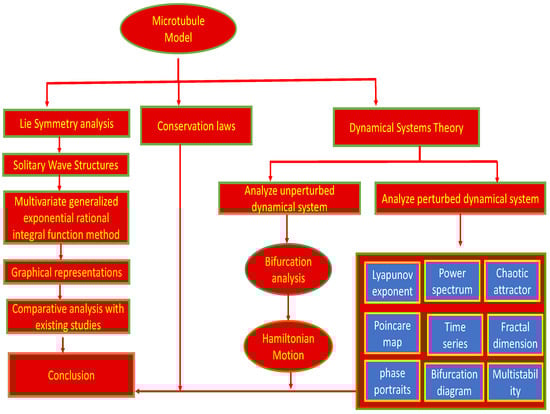
Figure 1. Graphical abstract illustrating the overall methodology and key findings of the proposed study.

2. Exploring Lie Symmetries of Equation (1)

Examine the Equation (1), which is presumed to remain unchanged under the following continuous point transformations [24]:

$$\begin{array}{cc}\hfill \overline{\alpha }=& \alpha +\varsigma {\zeta }^1(\alpha ,\mathfrak{T},\mathcal{J})+\mathfrak{O}\left({\varsigma }^2\right),\hfill \\ \hfill \overline{\mathfrak{T}}=& \mathfrak{T}+\varsigma {\zeta }^2(\alpha ,\mathfrak{T},\mathcal{J})+\mathfrak{O}\left({\varsigma }^2\right),\hfill \\ \hfill \overline{\mathcal{J}}=& \mathcal{J}+\varsigma \lambda (\alpha ,\mathfrak{T},\mathcal{J})+\mathfrak{O}\left({\varsigma }^2\right).\hfill \end{array}$$

(2)

Here, ${\zeta }^1$, ${\zeta }^1$, and $\lambda$ represent the infinitesimals, while ${\eta }_{\alpha ,t}$, ${\eta }_x$, ${\eta }_{xx}$, ${\eta }_{xxx}$, ${\eta }_{xxxx}$, and ${\eta }_{xxxxx}$ denote the corresponding prolongations of orders $\alpha ,1,2,3,4$, and 5, respectively. The group generator is given by

$$\mathrm{\Pi }={\zeta }^1(\alpha ,\mathfrak{T},\mathcal{J}){\displaystyle \frac{\partial }{\partial \alpha }}+{\zeta }^2(\alpha ,\mathfrak{T},\mathcal{J}){\displaystyle \frac{\partial }{\partial \mathfrak{T}}}+\lambda (\alpha ,\mathfrak{T},\mathcal{J}){\displaystyle \frac{\partial }{\partial \mathcal{U}}}.$$

(3)

Equation (1) admits the one-parameter Lie symmetry transformations (2), provided that the following invariance condition is satisfied:

$$\begin{array}{c}\hfill {\mathrm{\Pi }}^{\left[3\right]}({\mathrm{\Theta }}_2{\varrho }_0{p}^2{\mathcal{J}}_{\alpha \alpha \mathfrak{T}}+p^2{\mathcal{J}}_{\alpha \alpha }+2{\mathrm{\Theta }}_1{\varrho }_0\mathrm{\Delta }\mathcal{J}{\mathcal{J}}_{\mathfrak{T}}-{\mathrm{\Theta }}_1{\varrho }_0{\mathcal{J}}_{\mathfrak{T}}){|}_{Equation\left(1\right)=0}=0.\end{array}$$

(4)

${\mathrm{\Pi }}^{\left[3\right]}$ indicates that the third prolongation takes the following form:

$$\begin{array}{cc}\hfill & {\mathrm{\Pi }}^{\left[3\right]}=\mathrm{\Pi }+{\lambda }^{\mathfrak{T}}(\alpha ,\mathfrak{T},\mathcal{J}){\displaystyle \frac{\partial }{\partial {\mathcal{J}}_{\mathfrak{T}}}}+{\lambda }^{\alpha }(\alpha ,\mathfrak{T},\mathcal{J}){\displaystyle \frac{\partial }{\partial {\mathcal{J}}_{\alpha }}}+{\lambda }^{\mathfrak{T}\mathfrak{T}}(\alpha ,\mathfrak{T},\mathcal{J}){\displaystyle \frac{\partial }{\partial {\mathcal{J}}_{\mathfrak{T}\mathfrak{T}}}}+{\lambda }^{\mathfrak{T}\alpha }(\alpha ,\mathfrak{T},\mathcal{J}){\displaystyle \frac{\partial }{\partial {\mathcal{J}}_{\mathfrak{T}\alpha }}}\hfill \\ & +{\lambda }^{\alpha \alpha }(\alpha ,\mathfrak{T},\mathcal{J}){\displaystyle \frac{\partial }{\partial {\mathcal{J}}_{\alpha \alpha }}}+{\lambda }^{\alpha \alpha \mathfrak{T}}(\alpha ,\mathfrak{T},\mathcal{J}){\displaystyle \frac{\partial }{\partial {\mathcal{J}}_{\alpha \alpha \mathfrak{T}}}}.\hfill \end{array}$$

(5)

Here:

$$\begin{array}{cc}\hfill & {\lambda }^{\alpha }={\mathfrak{D}}_{\alpha }\left(\lambda \right)-{\mathcal{J}}_{\alpha }{\mathfrak{D}}_{\alpha }\left({\zeta }^1\right)-{\mathcal{J}}_{\mathfrak{T}}{\mathfrak{D}}_{\alpha }\left({\zeta }^2\right),\hfill \\ \hfill & {\lambda }^{\mathfrak{T}}={\mathfrak{D}}_{\mathfrak{T}}\left(\lambda \right)-{\mathcal{J}}_{\alpha }{\mathfrak{D}}_{\mathfrak{T}}\left({\zeta }^1\right)-{\mathcal{J}}_{\mathfrak{T}}{\mathfrak{D}}_{\mathfrak{T}}\left({\zeta }^2\right),\hfill \\ \hfill & {\lambda }^{\alpha \alpha }={\mathfrak{D}}_{\alpha }\left({\lambda }^{\alpha }\right)-{\mathcal{J}}_{\alpha \alpha }{\mathfrak{D}}_{\alpha }\left({\zeta }^1\right)-{\mathcal{J}}_{\mathfrak{T}\alpha }{\mathfrak{D}}_{\alpha }\left({\zeta }^2\right),\hfill \\ \hfill & {\lambda }^{\alpha \alpha \alpha }={\mathfrak{D}}_{\alpha }\left({\lambda }^{\alpha \alpha }\right)-{\mathcal{J}}_{\alpha \alpha \alpha }{\mathfrak{D}}_{\alpha }\left({\zeta }^1\right)-{\mathcal{J}}_{\mathfrak{T}\alpha \alpha }{\mathfrak{D}}_{\alpha }\left({\zeta }^2\right),\hfill \\ \hfill & {\lambda }^{\alpha \alpha \mathfrak{T}}={\mathfrak{D}}_{\alpha }\left({\lambda }^{\alpha \alpha }\right)-{\mathcal{J}}_{\alpha \alpha \mathfrak{T}}{\mathfrak{D}}_{\alpha }\left({\zeta }^1\right)-{\mathcal{J}}_{\mathfrak{T}\alpha \alpha }{\mathfrak{D}}_{\alpha }\left({\zeta }^2\right).\hfill \end{array}$$

(6)

Expanding Equation (5) and separating terms based on the derivatives of u results in the following system of determining equations obtained through symbolic computation.

$$\begin{array}{cc}\hfill & -2{\mathrm{\Theta }}_2{\varrho }_0{p}^2{\zeta }_{\mathcal{J}}^2=0,-{\mathrm{\Theta }}_2{\varrho }_0{p}^2{\zeta }_{\mathcal{J}}^2=0,-2{\mathrm{\Theta }}_2{\varrho }_0{p}^2{\zeta }_{\alpha }^2=0,-4{\mathrm{\Theta }}_2{\varrho }_0{p}^2{\zeta }_{\mathcal{J}\mathcal{J}}^2=0,-{\mathrm{\Theta }}_2{\varrho }_0{p}^2{\zeta }_{\mathcal{J}\mathcal{J}}^2=0,\hfill \\ \hfill & -4{\mathrm{\Theta }}_2{\varrho }_0{p}^2{\zeta }_{\alpha \mathcal{J}}^2=0,-2{\mathrm{\Theta }}_2{\varrho }_0{p}^2{\zeta }_{\alpha \mathcal{J}}^2=0,-{\mathrm{\Theta }}_2{\varrho }_0{p}^2{\zeta }_{\alpha \alpha }^2=0,-{\mathrm{\Theta }}_2{\varrho }_0{p}^2{\zeta }_{\mathcal{J}\mathcal{J}\mathcal{J}}^2=0,\hfill \\ & -2{\mathrm{\Theta }}_2{\varrho }_0{p}^2{\zeta }_{\alpha \mathcal{J}\mathcal{J}}^2=0,-{\mathrm{\Theta }}_2{\varrho }_0{p}^2{\zeta }_{\mathfrak{T}}^1=0,-3{\mathrm{\Theta }}_2{\varrho }_0{p}^2{\zeta }_{\mathcal{J}}^1=0,-{\mathrm{\Theta }}_2{\varrho }_0{p}^2{\zeta }_{\mathcal{J}}^1=0,-3{\mathrm{\Theta }}_2{\varrho }_0{p}^2{\zeta }_{\mathcal{J}\mathfrak{T}}^1=0,\hfill \\ \hfill & -3{\mathrm{\Theta }}_2{\varrho }_0{p}^2{\zeta }_{\mathcal{J}\mathcal{J}}^1=0,-{\mathrm{\Theta }}_2{\varrho }_0{p}^2{\zeta }_{\mathcal{J}\mathcal{J}\mathcal{J}}^1=0,-p^2{\zeta }_{\mathcal{J}\mathcal{J}}^1-{\mathrm{\Theta }}_2{\varrho }_0{p}^2{\zeta }_{\mathcal{J}\mathcal{J}\mathfrak{T}}^1=0,\hfill \\ \hfill & -2p^2{\zeta }_{\alpha \mathcal{J}}^2-{\mathrm{\Theta }}_2{\varrho }_0{p}^2{\zeta }_{\alpha \alpha \mathcal{J}}^1+2{\mathrm{\Theta }}_2{\varrho }_0{p}^2{\lambda }_{\alpha \mathcal{J}\mathcal{J}}-2{\mathrm{\Theta }}_2{\varrho }_0{p}^2{\zeta }_{\alpha \mathcal{J}\mathfrak{T}}^2+4{\varrho }_0\mathrm{\Delta }{\zeta }_{\mathcal{J}}^1{\mathrm{\Theta }}_1\mathcal{J}-2{\varrho }_0{\zeta }_{\mathcal{J}}^1\mathrm{\Theta }=0.\hfill \\ \hfill & -{\varrho }_0{\zeta }_{\mathcal{J}}^2\mathrm{\Theta }+2{\varrho }_0\mathrm{\Delta }{\zeta }_{\mathcal{J}}^2{\mathrm{\Theta }}_{1}u-{\mathrm{\Theta }}_2{\varrho }_0{p}^2{\zeta }_{\alpha \alpha \mathcal{J}}^2=0,-2p^2{\zeta }_{\mathcal{J}}^2-4{\mathrm{\Theta }}_2{\varrho }_0{p}^2{\zeta }_{\alpha \mathcal{J}}^1-2{\mathrm{\Theta }}_2{\varrho }_0{p}^2{\zeta }_{\mathcal{J}\mathfrak{T}}^2+2{\mathrm{\Theta }}_2{\varrho }_0{p}^2{\lambda }_{\mathcal{J}\mathcal{J}}=0,\hfill \\ \hfill & p^2{\zeta }_{\mathcal{J}}^2-2{\mathrm{\Theta }}_2{\varrho }_0{p}^2{\zeta }_{\alpha \mathcal{J}}^1-{\mathrm{\Theta }}_2{\varrho }_0{p}^2{\zeta }_{\mathcal{J}\mathfrak{T}}^2+{\mathrm{\Theta }}_2{\varrho }_0{p}^2{\lambda }_{\mathcal{J}\mathcal{J}}=0,\alpha -2{\mathrm{\Theta }}_2{\varrho }_0{p}^2{\zeta }_{\alpha \mathfrak{T}}^2+2{\mathrm{\Theta }}_2{\varrho }_0{p}^2{\lambda }_{\alpha \mathcal{J}}-{\mathrm{\Theta }}_2{\varrho }_0{p}^2{\zeta }_{\alpha \alpha }^1=0,\hfill \\ \hfill & -p^2{\zeta }_{\mathcal{J}\mathcal{J}}^2-2{\mathrm{\Theta }}_2{\varrho }_0{p}^2{\zeta }_{\alpha \mathcal{J}\mathcal{J}}^1+{\mathrm{\Theta }}_2{\varrho }_0{p}^2{\lambda }_{\mathcal{J}\mathcal{J}\mathcal{J}}-{\mathrm{\Theta }}_2{\varrho }_0{p}^2{\zeta }_{\mathcal{J}\mathcal{J}\mathfrak{T}}^2=0,-2p^2{\zeta }^2=0,\hfill \\ \hfill & -2p^2{\zeta }_{\alpha \mathcal{J}}^1+p^2{\lambda }_{\mathcal{J}\mathcal{J}}-2{\mathrm{\Theta }}_2{\varrho }_0{p}^2{\zeta }_{\alpha \mathcal{J}\mathfrak{T}}^1+{\mathrm{\Theta }}_2{\varrho }_0{p}^2{\lambda }_{\mathcal{J}\mathcal{J}\mathfrak{T}}=0,p^2{\zeta }_{\mathfrak{T}}^2-2{\mathrm{\Theta }}_2{\varrho }_0{p}^2{\zeta }_{\alpha \mathfrak{T}}^1+{\mathrm{\Theta }}_2{\varrho }_0{p}^2{\lambda }_{\mathcal{J}\mathfrak{T}}=0,\hfill \\ \hfill & {\mathrm{\Theta }}_2{\varrho }_0{p}^2{\lambda }_{\alpha \alpha \mathfrak{T}}-{\varrho }_0{\lambda }_{\mathfrak{T}}\mathrm{\Theta }+p^2{\lambda }_{\alpha \alpha }+2{\varrho }_0\mathrm{\Delta }{\lambda }_{\mathfrak{T}}{\mathrm{\Theta }}_1\mathcal{J}=0.\hfill \end{array}$$

(7)

The solutions to the aforementioned equations provide the corresponding infinitesimals:

$$\left\{\begin{array}{cc}\hfill & {\zeta }^1={\mathcal{E}}_3-\mathrm{\Delta }{\mathcal{E}}_2\alpha ,\hfill \\ \hfill & {\zeta }^2={\mathcal{E}}_1,\hfill \\ \hfill & \lambda =2\mathrm{\Delta }{\mathcal{E}}_2\mathcal{J}-{\mathcal{E}}_2.\hfill \end{array}\right.$$

(8)

Considering the arbitrary constants ${\mathcal{E}}_q$ ($q=1,2,3$), the Lie algebra of the microtubule equation is generated by the following three Lie symmetry operators.

$$\left\{\begin{array}{cc}\hfill & {\mathrm{\Pi }}_1={\displaystyle \frac{\partial }{\partial \alpha }}\hfill \\ \hfill & {\mathrm{\Pi }}_2={\displaystyle \frac{\partial }{\partial \mathfrak{T}}},\hfill \\ \hfill & {\mathrm{\Pi }}_3=(-1+2\mathrm{\Delta }\mathcal{J}){\displaystyle \frac{\partial }{\partial \mathcal{J}}}-\mathrm{\Delta }\alpha {\displaystyle \frac{\partial }{\partial \alpha }}.\hfill \end{array}\right.$$

(9)

Remark 1. 

The one-parameter Lie symmetry groups $\mathcal{B}\left(\varsigma \right)$, generated by ${\mathcal{E}}_q$ ($q=1,2,3$), are given as follows:

$$\begin{array}{cc}\hfill & {\mathcal{B}}_{1a}:(\alpha ,\mathfrak{T},\mathcal{J})\to (\alpha +\varsigma ,\mathfrak{T},\mathcal{J}),\hfill \\ \hfill & {\mathcal{B}}_{2a}:(\alpha ,\mathfrak{T},\mathcal{J})\to (\alpha ,\mathfrak{T}+\varsigma ,\mathcal{J})\hfill \\ \hfill & {\mathcal{B}}_{3a}:(\alpha ,\mathfrak{T},\mathcal{J})\to \left(e^{-\mathrm{\Delta }\varsigma }\alpha ,\mathfrak{T},{\displaystyle \frac{1+2e^{2\mathrm{\Delta }\varsigma }(\mathrm{\Delta }\mathcal{J}-1)}{\mathrm{\Delta }}}\right).\hfill \end{array}$$

(10)

Remark 2. 

If $\mathcal{J}(\alpha ,\mathfrak{T})$ is a valid solution of Equation (1), then an additional solution takes the following form:

$$\begin{array}{c}\hfill \begin{array}{c}\hfill \begin{array}{cc}& {\mathcal{B}}_{1b}:(\alpha ,\mathfrak{T})\to (\alpha -\varsigma ,\mathfrak{T}),\hfill \\ & {\mathcal{B}}_{2b}:(\alpha ,\mathfrak{T})\to (\alpha ,\mathfrak{T}-\varsigma )\hfill \\ & {\mathcal{B}}_{3b}:(\alpha ,\mathfrak{T})\to \mathcal{J}\left(e^{\mathrm{\Delta }\varsigma }\varsigma ,\mathfrak{T}\right)+{\displaystyle \frac{\mathrm{\Delta }\mathcal{J}-1+e^{2\mathrm{\Delta }\varsigma }}{\mathrm{\Delta }{e}^{2\mathrm{\Delta }\varsigma }}}.\hfill \end{array}\end{array}\end{array}$$

(11)

3. Symmetry Reduction of Equation (1)

The next section explores the symmetries and reductions of the microtubule equation. By choosing suitable coordinates, the equation is simplified by reducing dependent variables. Converting the PDE into an ODE or a simpler PDE is achieved by reducing independent parameters. In the $(\alpha ,\mathfrak{T},\mathcal{J})$ framework, the equation transforms into an ODE in $(\mathcal{H},\Psi )$, with simplification obtained via the chain rule.

Preposition 1. 

The solution $\mathcal{J}(\alpha ,\mathfrak{T})={\mathfrak{K}}_1\alpha +{\mathfrak{K}}_2$ is the solution of Equation (1) using the operator ${\mathrm{\Pi }}_1$.

Proof. 

The characteristic equation is expressed using ${\mathrm{\Pi }}_1$ in the following manner:

$${\displaystyle \frac{d\alpha }{1}}={\displaystyle \frac{d\mathfrak{T}}{0}}={\displaystyle \frac{d\mathcal{J}}{0}}.$$

(12)

The similarity variables for Equation (12) are given as follows:

$$\mathcal{J}=\mathcal{H}(\Psi ),\Psi =\mathfrak{T}.$$

(13)

Substituting Equation (13) into Equation (12), we obtain the following ODE:

$$p^2{\mathcal{H}}^{\prime \prime }=0.$$

(14)

By integrating Equation (14) twice with respect to $\Psi$, we obtain the following:

$$\mathcal{H}(\Psi )={\mathfrak{K}}_1\Psi +{\mathfrak{K}}_2.$$

(15)

The back-substituting the value of $\Psi$ in Equation (15), we obtain the solution of Equation (1):

$$\mathcal{J}(\alpha ,\mathfrak{T})={\mathfrak{K}}_1\alpha +{\mathfrak{K}}_2.$$

□

Preposition 2. 

The solution $\mathcal{J}(\alpha ,\mathfrak{T})={\displaystyle \frac{1}{2\mathrm{\Delta }}}$ or $\mathcal{J}(\alpha ,\mathfrak{T})=-{\mathfrak{K}}_3$ is the solution of Equation (1) using the operator ${\mathrm{\Pi }}_2$.

Proof. 

The characteristic equation, formulated with ${\mathrm{\Pi }}_2$, takes the following form:

$${\displaystyle \frac{d\alpha }{0}}={\displaystyle \frac{d\mathfrak{T}}{1}}={\displaystyle \frac{d\mathcal{J}}{0}}.$$

(16)

Equation (16) has the following similarity variables:

$$\mathcal{J}=\mathcal{H}(\Psi ),\Psi =\alpha .$$

(17)

By applying Equation (13) to Equation (12), the resulting ODE is as follows:

$${\mathrm{\Theta }}_1{\varrho }_0\left({\mathcal{J}}^{\prime }\right)(2\mathrm{\Delta }{\mathcal{J}}^{\prime }-1)=0.$$

(18)

The solution of Equation (18) is given by the following:

$$\mathcal{H}(\Psi )={\displaystyle \frac{1}{2\mathrm{\Delta }}},\mathrm{or}\mathcal{H}(\Psi )=-{\mathfrak{K}}_3.$$

(19)

After applying the inverse transformation, the solution of Equation (1) is obtained as follows:

$$\mathcal{J}(\alpha ,\mathfrak{T})={\displaystyle \frac{1}{2\mathrm{\Delta }}},\mathrm{or}\mathcal{J}(\alpha ,\mathfrak{T})=-{\mathfrak{K}}_3.$$

(20)

□

Preposition 3. 

The solution $\mathcal{J}(\alpha ,\mathfrak{T})=e^{{\displaystyle \frac{-LambertW\left(\frac{\mathrm{\Delta }{\mathrm{\Theta }}_1{e}^{\frac{-h_1}{{\mathrm{\Theta }}_2{\varrho }_0}-\frac{\mathfrak{T}}{{\mathrm{\Theta }}_2{\varrho }_0}}}{3p^2{\mathrm{\Theta }}_2}\right){\mathrm{\Theta }}_2{\varrho }_0+c_1+\mathfrak{T}}{{\mathrm{\Theta }}_2{\varrho }_0}}}$ is the solution of Equation (1) using the operator ${\mathrm{\Pi }}_3$.

Proof. 

Utilizing ${\mathrm{\Pi }}_3$, the characteristic equation is presented as follows:

$${\displaystyle \frac{d\alpha }{-\mathrm{\Delta }\alpha }}={\displaystyle \frac{d\mathfrak{T}}{0}}={\displaystyle \frac{d\mathcal{J}}{-1+2\mathrm{\Delta }\mathcal{J}}}.$$

(21)

The similarity variables corresponding to Equation (21) are presented below:

$$\mathcal{J}=\mathcal{H}(\Psi ),\Psi ={\displaystyle \frac{{\alpha }^2+2\mathrm{\Delta }\mathcal{H}\left(\xi \right)}{2\mathrm{\Delta }{\alpha }^2}},\xi =\mathfrak{T}.$$

(22)

Incorporating Equation (22) into Equation (12), we derive the following ODE:

$$2{\mathrm{\Theta }}_1{\varrho }_0\mathrm{\Delta }\mathcal{H}{\mathcal{H}}^{\prime }+6{\mathrm{\Theta }}_1{\varrho }_0{p}^2{\mathcal{H}}^{\prime }+6p^2\mathcal{H}=0.$$

(23)

Solve Equation (23) using Maple software to obtain the solution of Equation (1) in the following form:

$$\mathcal{J}(\alpha ,\mathfrak{T})=e^{{\displaystyle \frac{-LambertW\left(\frac{\mathrm{\Delta }{\mathrm{\Theta }}_1{e}^{\frac{-h_1}{{\mathrm{\Theta }}_2{\varrho }_0}-\frac{\mathfrak{T}}{{\mathrm{\Theta }}_2{\varrho }_0}}}{3p^2{\mathrm{\Theta }}_2}\right){\mathrm{\Theta }}_2{\varrho }_0+c_1+\mathfrak{T}}{{\mathrm{\Theta }}_2{\varrho }_0}}}.$$

(24)

□

4. Analytical Solutions for the Equation (1)

In this section, we describe the general procedure of the MGERIFM and apply it to the microtubule equation.

4.1. Methodology of MGERIFM

This section presents the MGERIFM, an efficient approach for obtaining novel analytical solutions to NLPDEs. MGERIFM serves as a powerful tool for solving complex mathematical problems [3]. Inital step: NLPDEs are typically represented as:

$$\mathfrak{Q}(\mathcal{J},{\mathcal{J}}_{\alpha },{\mathcal{J}}_{\mathfrak{T}},{\mathcal{J}}_{\alpha \alpha },{\mathcal{J}}_{\alpha \mathfrak{T}},{\mathcal{J}}_{\mathfrak{T}\mathfrak{T}},\dots )=0.$$

(25)

Step 2: To simplify Equation (25), we apply the following transformation:

$$\mathcal{J}=\mathcal{H}(\Psi ),\Psi =\alpha -\eta \mathfrak{T}.$$

(26)

Here, $\eta$ shows the wave speed of the soliton. Substituting transformation (26) into (25), the resulting nonlinear ordinary differential equation takes the form [3]:

$$\mathfrak{S}(\mathcal{H},{\mathcal{H}}^{\prime },{\mathcal{H}}^{\prime \prime },{\mathcal{H}}^{\prime \prime \prime },{\mathcal{H}}^{\prime \prime \prime \prime },{\mathcal{H}}^{\prime \prime \prime \prime \prime },\dots )=0,$$

(27)

where ${\mathcal{H}}^{\prime }={\displaystyle \frac{d\mathcal{H}}{d\Psi }}$, ${\mathcal{H}}^{\prime \prime }={\displaystyle \frac{d^2\mathcal{H}}{d{\Psi }^2}}$, ${\mathcal{H}}^{\prime }={\displaystyle \frac{d^3\mathcal{H}}{d{\Psi }^3}}$, and so on.

Step 3: Consider

$$\mathcal{H}(\Psi )={\mathcal{V}}_0+\sum _{s=1}^{\mathcal{L}}{\mathcal{V}}_s{\left(\underset{s}{\underbrace{\int \int \dots \int }}\mathcal{M}(\Psi )d\Psi d\Psi \dots d\Psi \right)}^s+\sum _{s=1}^{\mathcal{L}}{\mathcal{G}}_s{\left(\underset{s}{\underbrace{\int \int \dots \int }}\mathcal{M}(\Psi )d\Psi d\Psi \dots d\Psi \right)}^{-s}.$$

(28)

Here,

$$\mathcal{M}(\Psi )={\displaystyle \frac{h_1{e}^{n_1\Psi }+h_2{e}^{n_2\Psi }}{h_3{e}^{n_3\Psi }+h_3{e}^{n_3\Psi }}}.$$

(29)

Step 4: The order $\mathcal{L}$ is determined using the homogeneous balancing principle between the highest derivative and nonlinear terms in Equation (27).

Step 5: Substituting Equation (28) into Equation (27) with Equation (29) yields the algebraic equation $\mathcal{A}({\mu }_1,{\mu }_2,{\mu }_3,{\mu }_4)=0$, where ${\mu }_q=e^{n_q\Psi }$ for $1\le q\le 4$. Then, each coefficient in $\mathcal{A}$ is set to zero.

Step 6: Using Maple, we compute the values of ${\mathcal{V}}_0$, ${\mathcal{V}}_s$, and ${\mathcal{G}}_s$ ($1\le s\le \mathcal{L}$), which are then substituted into Equations (28) and (29) to derive exact soliton solutions for Equation (27).

4.2. Analytical Solutions of the Equation (1) via MGERIFM

Considering wave transfornmation:

$$\mathcal{J}(\alpha ,\mathfrak{T})=\mathcal{H}(\Psi ),\Psi =\alpha -\eta \mathfrak{T}.$$

(30)

Applying the transformation Equation (30) to Equation (1), we obtain:

$$-{\mathrm{\Theta }}_2{\varrho }_0{p}^2{\mathcal{H}}^{\prime \prime \prime }\eta +p^2{\mathcal{H}}^{\prime \prime }-2{\mathrm{\Theta }}_1{\varrho }_0\mathrm{\Delta }{\mathcal{H}}^{\prime }\eta \mathcal{H}+{\mathrm{\Theta }}_1{\varrho }_0{\mathcal{H}}^{\prime }\eta =0.$$

(31)

Integrating Equation (31), we obtain the second-order ODE:

$$-{\mathrm{\Theta }}_2{\varrho }_0{p}^2{\mathcal{H}}^{\prime \prime }\eta +p^2{\mathcal{H}}^{\prime }-2{\mathrm{\Theta }}_1{\varrho }_0\mathrm{\Delta }\eta {\mathcal{H}}^2+{\mathrm{\Theta }}_1{\varrho }_0\eta \mathcal{H}=0.$$

(32)

By balancing the terms ${\mathcal{H}}^{\prime \prime }$ and ${\mathcal{H}}^2$ in Equation (32), we find $\mathcal{L}=2$, leading to the following trial solution:

$$\mathcal{H}(\Psi )={\mathcal{V}}_0+{\mathcal{V}}_1\left(\int \mathcal{M}(\Psi )d\Psi \right)+{\mathcal{V}}_2{\left(\int \int \mathcal{M}(\Psi )d\Psi d\Psi \right)}^2+{\displaystyle \frac{{\mathcal{G}}_1}{\int \mathcal{M}(\Psi )d\Psi }}+{\displaystyle \frac{{\mathcal{G}}_2}{{\left(\int \int \mathcal{M}(\Psi )d\Psi d\Psi \right)}^2}}.$$

(33)

By inserting Equation (26) into Equation (32) and utilizing the MGERIFM with computational tools like Maple 2023, we derive a set of solutions for the microtubule equation [26,27].

4.2.1. Established Sine Representation

By assigning the parameters $h_1=1,h_2=-1,h_3=h_4=i$ and $n_1=i,n_2=-i,$$n_3=n_4=0$, Equation (29) simplifies to the standard sine function form:

$$\mathcal{M}(\Psi )=\sin (\Psi ).$$

(34)

By substituting Equation (34) into Equation (33), the expression for $\mathcal{H}\left(\vartheta \right)$ is derived:

$$\mathcal{H}(\Psi )={\mathcal{V}}_0-{\mathcal{V}}_1\cos (\Psi )+{\mathcal{V}}_2{\sin }^2(\Psi )-{\mathcal{G}}_1\sec (\Psi )+{\mathcal{G}}_2{\csc }^2(\Psi ).$$

(35)

Substituting Equation (35) into Equation (32) results in an algebraic system. By comparing the coefficients of the trigonometric terms, we obtain the following solution:

Family 5.1.a: ${\mathcal{V}}_0\ne 0,{\mathcal{V}}_1=0,{\mathcal{V}}_2\ne 0,{\mathcal{G}}_1\ne 0,{\mathcal{G}}_2\ne 0,{\mathrm{\Theta }}_1=0,p=0.$

By inserting the given constants into Equation (35), we obtain the solution for Equation (32) as follows.

$$\mathcal{H}(\Psi )={\mathcal{V}}_0+{\mathcal{V}}_2\sin (\Psi )-{\mathcal{G}}_1\sec (\Psi )+{\mathcal{G}}_2{\csc }^2(\Psi ).$$

(36)

Thus, substituting Equation (36) into Equation (30) yields the exact invariant solution for the microtubule equation [28,29]:

$${\mathcal{J}}_1(\alpha ,\mathfrak{T})=-{\displaystyle \frac{{\mathcal{V}}_2}{4}}{e}^{2i(\eta \mathfrak{T}-\alpha )}-{\displaystyle \frac{{\mathcal{V}}_2}{4}}{e}^{2i(\alpha -\eta \mathfrak{T})}-{\displaystyle \frac{4{\mathcal{G}}_2{e}^{2i(\eta \mathfrak{T}+\alpha )}}{{\left(e^{2i\alpha }-e^{2i\eta \mathfrak{T}}\right)}^2}}-{\displaystyle \frac{2{\mathcal{G}}_1{e}^{i(\eta \mathfrak{T}+\alpha )}}{e^{2i\eta \mathfrak{T}}+e^{2i\alpha }}}+{\mathcal{V}}_0+{\displaystyle \frac{{\mathcal{V}}_2}{2}}$$

(37)

Family 5.1.b: ${\mathcal{V}}_1=0,{\mathcal{V}}_2=0,{\mathcal{V}}_0\ne 0,{\mathcal{G}}_1=0,{\mathrm{\Theta }}_1=0,p=0,{\mathcal{G}}_2\ne 0.$

By inserting the given constants into Equation (35), we obtain the solution for Equation (32) as follows.

$$\mathcal{H}(\Psi )={\mathcal{V}}_0+{\mathcal{G}}_2{\csc }^2(\Psi ).$$

(38)

Thus, substituting Equation (38) into Equation (30) yields the exact invariant solution for the microtubule equation:

$${\mathcal{J}}_2(\alpha ,\mathfrak{T})={\mathcal{V}}_0-{\displaystyle \frac{4{\mathcal{G}}_2{e}^{2i(\eta \mathfrak{T}+\alpha )}}{{\left(e^{2i\alpha }-e^{2i\eta \mathfrak{T}}\right)}^2}}.$$

(39)

Family 5.1.c: ${\mathcal{V}}_0\ne 0,{\mathcal{V}}_1\ne 0,{\mathcal{V}}_2\ne 0,{\mathcal{G}}_1=0,{\mathcal{G}}_2\ne 0,{\mathrm{\Theta }}_1=0,p=0.$

By inserting the given constants into Equation (35), we obtain the solution for Equation (32) as follows.

$$\mathcal{H}(\Psi )={\mathcal{V}}_0+{\mathcal{V}}_2{\sin }^2(\Psi )+{\mathcal{G}}_2{\csc }^2(\Psi ).$$

(40)

Thus, substituting Equation (40) into Equation (30) yields the exact invariant solution for the microtubule equation:

$${\mathcal{J}}_3(\alpha ,\mathfrak{T})=-{\displaystyle \frac{{\mathcal{V}}_2}{4}}{e}^{2i(\eta \mathfrak{T}-\alpha )}-{\displaystyle \frac{{\mathcal{V}}_2}{4}}{e}^{2i(\alpha -\eta \mathfrak{T})}-{\displaystyle \frac{4{\mathcal{G}}_2{e}^{2i(\eta \mathfrak{T}+\alpha )}}{{\left(e^{2i\alpha }-e^{2i\eta \mathfrak{T}}\right)}^2}}+{\mathcal{V}}_0+{\displaystyle \frac{{\mathcal{V}}_2}{2}}.$$

(41)

4.2.2. Established Cosine Representation:

By setting the parameters as $h_1=h_2=h_3=h_4=1$ and $n_1=i,n_2=-i,$$n_3=n_4=0$, Equation (29) reduces to the conventional cosine function form:

$$\mathcal{M}(\Psi )=\cos (\Psi ).$$

(42)

By substituting Equation (42) into Equation (33), the expression for $\mathcal{H}\left(\vartheta \right)$ is derived:

$$\mathcal{H}(\Psi )={\mathcal{V}}_0+{\mathcal{V}}_1\sin (\Psi )+{\mathcal{V}}_2{\cos }^2(\Psi )+{\mathcal{G}}_1\csc (\Psi )+{\mathcal{G}}_2{\sec }^2(\Psi ).$$

(43)

Family 5.2.a: ${\mathcal{V}}_0\ne 0,{\mathcal{V}}_1=0,{\mathcal{V}}_2\ne 0,{\mathcal{G}}_1\ne 0,{\mathcal{G}}_2\ne 0,{\mathrm{\Theta }}_1=0,p=0.$

By inserting the given constants into Equation (43), we obtain the solution for Equation (32) as follows.

$$\mathcal{H}(\Psi )={\mathcal{V}}_0+{\mathcal{V}}_2{\cos }^2(\Psi )+{\mathcal{G}}_1\csc (\Psi )+{\mathcal{G}}_2{\sec }^2(\Psi ).$$

(44)

Thus, substituting Equation (44) into Equation (30) yields the exact invariant solution for the microtubule equation:

$${\mathcal{J}}_4(\alpha ,\mathfrak{T})={\displaystyle \frac{{\mathcal{V}}_2}{4}}{\left(e^{i(\alpha -\eta \mathfrak{T})}+e^{i(\eta \mathfrak{T}-\alpha )}\right)}^2+{\displaystyle \frac{2i{\mathcal{G}}_1}{e^{i(\alpha -\eta \mathfrak{T})}-e^{i(\eta \mathfrak{T}-\alpha )}}}+{\displaystyle \frac{4{\mathcal{G}}_2{e}^{2i(\eta \mathfrak{T}+\alpha )}}{{\left(e^{2i\eta \mathfrak{T}}+e^{2i\alpha }\right)}^2}}+{\mathcal{V}}_0.$$

(45)

Family 5.2.b: ${\mathcal{V}}_0\ne 0,{\mathcal{V}}_1\ne 0,{\mathcal{V}}_2\ne 0,{\mathcal{G}}_1=0,{\mathcal{G}}_2\ne 0,{\mathrm{\Theta }}_1=0,p=0.$

By inserting the given constants into Equation (43), we obtain the solution for Equation (32) as follows.

$$\mathcal{H}(\Psi )={\mathcal{V}}_2{\cos }^2(\Psi )+{\mathcal{G}}_2{\sec }^2(\Psi )+{\mathcal{V}}_0.$$

(46)

Thus, substituting Equation (46) into Equation (30) yields the exact invariant solution for the microtubule equation:

$${\mathcal{J}}_5(\alpha ,\mathfrak{T})={\displaystyle \frac{{\mathcal{V}}_2}{4}}{\left(e^{i(\alpha -\eta \mathfrak{T})}+e^{i(\eta \mathfrak{T}-\alpha )}\right)}^2+{\displaystyle \frac{4{\mathcal{G}}_2{e}^{2i(\eta \mathfrak{T}+\alpha )}}{{\left(e^{2i\eta \mathfrak{T}}+e^{2i\alpha }\right)}^2}}+{\mathcal{V}}_0.$$

(47)

Family 5.2.c: ${\mathcal{V}}_0\ne 0,{\mathcal{V}}_1\ne 0,{\mathcal{V}}_2\ne 0,{\mathcal{G}}_1\ne 0,{\mathcal{G}}_2=0,{\mathrm{\Theta }}_1=0,p=0.$

By inserting the given constants into Equation (43), we obtain the solution for Equation (32) as follows.

$$\mathcal{H}(\Psi )={\mathcal{V}}_2{\cos }^2(\Psi )+{\mathcal{V}}_0.$$

(48)

Thus, substituting Equation (48) into Equation (30) yields the exact invariant solution for the microtubule equation:

$${\mathcal{J}}_6(\alpha ,\mathfrak{T})={\mathcal{V}}_0+{\displaystyle \frac{{\mathcal{V}}_2}{4}}{e}^{-2i(\eta \mathfrak{T}+\alpha )}{\left(e^{2i\eta \mathfrak{T}}+e^{2i\alpha }\right)}^2.$$

(49)

4.2.3. Established Exponential Representation

By setting the parameters as $h_1=h_2=h_3=h_4=2$ and $n_1=n_2={\displaystyle \frac{2}{5}},n_3=n_4=0$, Equation (29) reduces to the conventional exponential function form:

$$\mathcal{M}(\Psi )=\exp \left({\displaystyle \frac{2\Psi }{5}}\right).$$

(50)

By substituting Equation (50) into Equation (33), the expression for $\mathcal{H}\left(\vartheta \right)$ is derived:

$$\mathcal{H}(\Psi )={\mathcal{V}}_0+{\displaystyle \frac{5}{2}}{\mathcal{V}}_1\exp \left({\displaystyle \frac{2\Psi }{5}}\right)+{\displaystyle \frac{625}{16}}{\mathcal{V}}_2\exp \left({\displaystyle \frac{4\Psi }{5}}\right)+{\displaystyle \frac{2}{5}}{\mathcal{G}}_1\exp \left({\displaystyle \frac{-2\Psi }{5}}\right)+{\displaystyle \frac{16}{625}}{\mathcal{G}}_2\exp \left({\displaystyle \frac{-4\Psi }{5}}\right).$$

(51)

Case 5.3.a: ${\mathcal{V}}_0=-{\displaystyle \frac{1-\sqrt{1-32{\mathrm{\Delta }}^2{\mathcal{V}}_1{\mathcal{G}}_1}}{4\mathrm{\Delta }}},{\mathcal{V}}_1\ne 0,{\mathcal{V}}_2=0,{\mathcal{G}}_1\ne 0,{\mathcal{G}}_2=0,{\mathrm{\Theta }}_1=0,p=0.$

By inserting the given constants into Equation (51), we obtain the solution for Equation (32) as follows.

$$\mathcal{H}(\Psi )={\displaystyle \frac{5{\mathcal{V}}_1}{2}}{e}^{{\displaystyle \frac{2\Psi }{5}}}-{\displaystyle \frac{1-\sqrt{1-32{\mathrm{\Delta }}^2{\mathcal{V}}_1{\mathcal{G}}_1}}{4\mathrm{\Delta }}}+{\displaystyle \frac{2{\mathcal{G}}_1}{5}}{e}^{-{\displaystyle \frac{2\Psi }{5}}}.$$

(52)

Thus, substituting Equation (52) into Equation (30) yields the exact invariant solution for the microtubule equation:

$${\mathcal{J}}_8(\alpha ,\mathfrak{T})={\displaystyle \frac{5{\mathcal{V}}_1}{2}}{e}^{{\displaystyle \frac{2(\alpha -\eta \mathfrak{T})}{5}}}-{\displaystyle \frac{1-\sqrt{1-32{\mathrm{\Delta }}^2{\mathcal{V}}_1{\mathcal{G}}_1}}{4\mathrm{\Delta }}}+{\displaystyle \frac{2{\mathcal{G}}_1}{5}}{e}^{-{\displaystyle \frac{2(\alpha -\eta \mathfrak{T})}{5}}}.$$

(53)

Family 5.3.b: ${\mathcal{V}}_0=0,{\mathcal{V}}_1\ne 0,{\mathcal{V}}_2=0,{\mathcal{G}}_1=0,{\mathcal{G}}_2=0,{\mathrm{\Theta }}_1=0,p={\displaystyle \frac{-5\sqrt{{\mathrm{\Theta }}_1\eta {\rho }_0}}{\sqrt{4\eta {\mathrm{\Theta }}_2\rho -10}}}.$

By inserting the given constants into Equation (51), we obtain the solution for Equation (32) as follows.

$$\mathcal{H}(\Psi )={\displaystyle \frac{5{\mathcal{V}}_1}{2}}{e}^{{\displaystyle \frac{2\Psi }{5}}}.$$

(54)

Thus, substituting Equation (54) into Equation (30) yields the exact invariant solution for the microtubule equation:

$${\mathcal{J}}_9(\alpha ,\mathfrak{T})={\displaystyle \frac{5{\mathcal{V}}_1}{2}}{e}^{{\displaystyle \frac{2(\alpha -\eta \mathfrak{T})}{5}}}.$$

(55)

4.2.4. Established Cosine Hyperbolic Representation

By assigning the parameters as $h_1=h_2=h_3=h_4=i$ and $n_1=1,n_2=-1,$$n_3=n_4=0$, Equation (29) reduces to the conventional hyperbolic cosine function form:

$$\mathcal{M}(\Psi )=\cosh (\Psi ).$$

(56)

By substituting Equation (62) into Equation (33), the expression for $\mathcal{H}\left(\vartheta \right)$ is derived:

$$\mathcal{H}(\Psi )={\mathcal{V}}_0+{\mathcal{V}}_1\sinh (\Psi )+{\mathcal{V}}_2{\cosh }^2(\Psi )+{\mathcal{G}}_1\mathrm{csch}(\Psi )+{\mathcal{G}}_2{\mathrm{sech}}^2(\Psi ).$$

(57)

Family 5.4.a: ${\mathcal{V}}_0\ne 0,{\mathcal{V}}_1\ne 0,{\mathcal{V}}_2\ne 0,{\mathcal{G}}_1\ne 0,{\mathcal{G}}_2=0,p=0.$

By inserting the given constants into Equation (57), we obtain the solution for Equation (32) as follows.

$$\mathcal{H}(\Psi )={\mathcal{V}}_0+{\mathcal{V}}_1\sinh (\Psi )+{\mathcal{V}}_2{\cosh }^2(\Psi )+{\mathcal{G}}_1\mathrm{csch}(\Psi ).$$

(58)

Thus, substituting Equation (58) into Equation (30) yields the exact invariant solution for the microtubule equation:

$${\mathcal{J}}_{10}(\alpha ,\mathfrak{T})={\mathcal{V}}_0-{\displaystyle \frac{{\mathcal{V}}_1}{2}}{e}^{-\Psi }+{\displaystyle \frac{e^{\Psi }{\mathcal{V}}_1}{2}}+{\displaystyle \frac{{\mathcal{V}}_2{e}^{-2\Psi }}{4}}+{\displaystyle \frac{{\mathcal{V}}_2{e}^{2\Psi }}{4}}+{\displaystyle \frac{{\mathcal{V}}_2}{2}}+{\displaystyle \frac{2i{e}^{i\Psi }{\mathcal{G}}_1}{-1+e^{2i\Psi }}}.$$

(59)

Family 5.4.b: ${\mathcal{V}}_0\ne 0,{\mathcal{V}}_1=0,{\mathcal{G}}_2\ne 0,p=0,{\mathrm{\Theta }}_1=0.$

By inserting the given constants into Equation (57), we obtain the solution for Equation (32) as follows.

$$\mathcal{H}(\Psi )={\mathcal{V}}_0+{\mathcal{G}}_2{\mathrm{csch}}^2(\Psi ).$$

(60)

Thus, substituting Equation (60) into Equation (30) yields the exact invariant solution for the microtubule equation:

$${\mathcal{J}}_{11}(\alpha ,\mathfrak{T})={\mathcal{V}}_0+{\displaystyle \frac{e^{-2(\alpha -\eta \mathfrak{T}){\mathcal{G}}_2}}{4}}{\left(e^{2(\alpha -\eta \mathfrak{T})}+1\right)}^2.$$

(61)

4.2.5. Established Sine Hyperbolic Representation

By assigning the parameters as $h_1=2i,h_2=-2i,h_3=h_4=4i$ and $n_1={\displaystyle \frac{1}{2}},n_2={\displaystyle \frac{-1}{2}},n_3=n_4=0$, Equation (29) reduces to the conventional hyperbolic sine function form:

$$\mathcal{M}(\Psi )={\displaystyle \frac{1}{2}}\sinh \left({\displaystyle \frac{\Psi }{2}}\right).$$

(62)

By substituting Equation (62) into Equation (33), the expression for $\mathcal{H}\left(\vartheta \right)$ is derived:

$$\mathcal{H}(\Psi )={\mathcal{V}}_0+{\mathcal{V}}_1\cosh \left({\displaystyle \frac{\Psi }{2}}\right)+4{\mathcal{V}}_2{\sinh }^2\left({\displaystyle \frac{\Psi }{2}}\right)+{\mathcal{Z}}_1\mathrm{sech}\left({\displaystyle \frac{\Psi }{2}}\right)+{\displaystyle \frac{{\mathcal{Z}}_2}{4}}{\mathrm{csch}}^2\left({\displaystyle \frac{\Psi }{2}}\right)$$

(63)

Family 5.4.a: ${\mathcal{V}}_0\ne 0,{\mathcal{V}}_1\ne 0,{\mathcal{V}}_2\ne 0,{\mathcal{G}}_1\ne 0,{\mathcal{G}}_2=0,p=0.$

By inserting the given constants into Equation (63), we obtain the solution for Equation (32) as follows.

$$\mathcal{H}(\Psi )={\mathcal{V}}_0+{\mathcal{V}}_1\cosh \left({\displaystyle \frac{\Psi }{2}}\right)+2{\mathcal{V}}_2(\cosh (\Psi )-1)+{\mathcal{G}}_1\mathrm{sech}\left({\displaystyle \frac{\Psi }{2}}\right).$$

(64)

Thus, substituting Equation (64) into Equation (30) yields the exact invariant solution for the microtubule equation:

$${\mathcal{J}}_{12}(\alpha ,\mathfrak{T})={\mathcal{V}}_0+{\displaystyle \frac{{\mathcal{V}}_1}{2}}{e}^{-{\displaystyle \frac{\Psi }{2}}}+{\displaystyle \frac{{\mathcal{V}}_1}{2}}{e}^{{\displaystyle \frac{\Psi }{2}}}+e^{-\Psi }{\mathcal{V}}_2+e^{\Psi }{\mathcal{V}}_2-2{\mathcal{V}}_2+{\displaystyle \frac{2e^{\frac{\Psi }{2}}{\mathcal{G}}_1}{e^{\Psi }+1}}.$$

(65)

Family 5.4.b: ${\mathcal{V}}_0\ne 0,{\mathcal{V}}_1\ne 0,{\mathcal{V}}_2=0,{\mathcal{G}}_1=0,{\mathcal{G}}_2=0,p=0.$

By inserting the given constants into Equation (63), we obtain the solution for Equation (32) as follows.

$$\mathcal{H}(\Psi )={\mathcal{V}}_0+{\mathcal{V}}_1\cosh \left({\displaystyle \frac{\Psi }{2}}\right).$$

(66)

Thus, substituting Equation (66) into Equation (30) yields the exact invariant solution for the microtubule equation:

$${\mathcal{J}}_{13}(\alpha ,\mathfrak{T})={\mathcal{V}}_0+{\displaystyle \frac{{\mathcal{V}}_1}{2}}{e}^{-{\displaystyle \frac{\Psi }{2}}}+{\displaystyle \frac{{\mathcal{V}}_1}{2}}{e}^{{\displaystyle \frac{\Psi }{2}}}.$$

(67)

5. Physical Interpretation of the Solutions

To enhance the understanding of the derived solutions, we present 3D surface plots alongside their corresponding contour diagrams. These graphical depictions offer valuable insights into the dynamic behavior of the solutions under specific parameter configurations. Figure 2, Figure 3, Figure 4, Figure 5 and Figure 6 display the lump profiles associated with different solutions, showcasing their real, imaginary, and absolute components under specific parameter choices and domains:

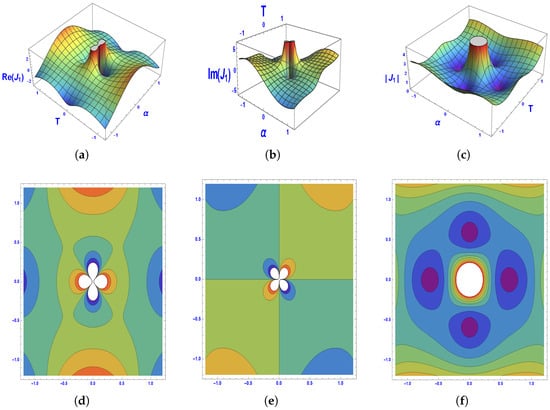
Figure 2. Visualization of the solution $J_1(\alpha ,\mathfrak{T})$ using 3D and contour plots.

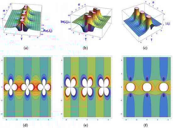
Figure 3. Graphical representation of the solution $J_2(\alpha ,\mathfrak{T})$ using 3D and contour plots.

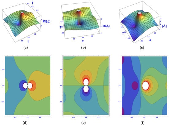
Figure 4. Graphical depiction of $J_4(\alpha ,\mathfrak{T})$ via 3D and contour plots.

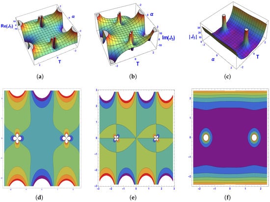
Figure 5. Graphical representation of 3D and contour plots of the solution $J_5(\alpha ,\mathfrak{T})$.

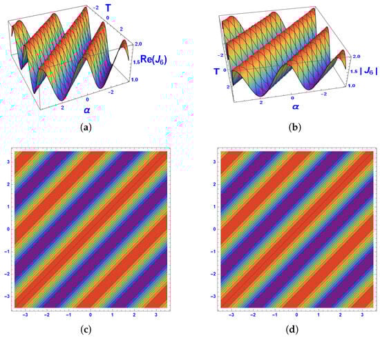
Figure 6. Graphical representation of 3D and contour plots of $J_6(\alpha ,\mathfrak{T})$ solution.

• Figure 2 illustrates the lump structures of solution (37) using the parameters ${\mathcal{V}}_0=0.56,{\mathcal{V}}_2=-0.47,{\mathcal{G}}_1=0.23,{\mathcal{G}}_2=0.045,\eta =\iota$, within the domain $\alpha ,\mathfrak{T}\in [-1.2,1.2]$. The figure reveals multi-soliton features evident in all three components of ${\mathcal{J}}_1(\alpha ,\mathfrak{T})$.
• Figure 3 presents the graphical structure of solution (39) based on the values ${\mathcal{V}}_0=0.26,{\mathcal{G}}_2=0.05,\eta =\iota$, over the range $\alpha ,\mathfrak{T}\in [-4.5,4.25]$. The solution ${\mathcal{J}}_2(\alpha ,\mathfrak{T})$ exhibits a similar solitonic nature in both real and complex planes.
• Figure 4 shows the lump characteristics of solution (53), obtained under ${\mathcal{V}}_0=0.56,$${\mathcal{V}}_2=0.47,{\mathcal{G}}_1=0.13,{\mathcal{G}}_2=2.5,\eta =\iota$, with $\alpha ,\mathfrak{T}\in [-0.9,0.9]$. The behavior of ${\mathcal{J}}_4(\alpha ,\mathfrak{T})$ reflects a multi-lump soliton profile across all observed components.
• Figure 5 depicts the profile of solution (47) with parameters ${\mathcal{V}}_0=0.16,{\mathcal{V}}_2=0.17,$${\mathcal{G}}_2=1.5,\eta =\iota$, within the domain $\alpha ,\mathfrak{T}\in [-2.9,2.9]$. The solution ${\mathcal{J}}_5(\alpha ,\mathfrak{T})$ maintains a similar localized pattern with distinct peak formations.
• Figure 6 represents the evolution of solution (49) for ${\mathcal{V}}_0=1.16,{\mathcal{V}}_2=1.17,\eta =\iota$, in the same spatial-temporal range as Figure 6. Unlike the previous figures, ${\mathcal{J}}_6(\alpha ,\mathfrak{T})$ here demonstrates periodic wave behavior with solitonic modulation.

Comprehension nonlinear wave propagation in a variety of physical systems requires an understanding of multi-soliton and periodic soliton solutions. The integrability and stability of the underlying nonlinear system are demonstrated by multi-solitons, which are complicated interactions between many solitary waves in which each wave maintains its shape and speed after colliding.

6. Conservation Laws of Equation (1)

This section presents symbols and theoretical concepts useful for deriving conservation laws based on the adjoint equation.

Theorem 1. 

Any form of Lie point symmetry, nonlocal symmetry, or Lie-Bäcklund symmetry:

$${\mathcal{B}}_1={\zeta }^m(\alpha ,\mathcal{J},{\mathcal{J}}_1,{\mathcal{J}}_2,\dots ){\partial }_{{\alpha }_m}+\lambda (\alpha ,\mathcal{J},{\mathcal{J}}_1,{\mathcal{J}}_2,\dots ){\partial }_{\mathcal{J}}.$$

(68)

The differential equation expressed in the following form:

$${\mathcal{B}}_1(\alpha ,\mathcal{J},{\mathcal{J}}_1,{\mathcal{J}}_2,\dots ,{\mathcal{J}}_{\left(w\right)})=0.$$

(69)

An adjoint equation retains the dependent variable $\mathcal{J}$ along with p independent variables $\alpha =({\alpha }_1,{\alpha }_2,\dots ,{\alpha }_p)$. Specifically, the corresponding operator is given by:

$$\mathcal{A}={\zeta }^m{\partial }_{{\alpha }_m}+\lambda {\partial }_{\mathcal{J}}+{\lambda }_{★}{\partial }_{\mathcal{Z}},$$

(70)

with an appropriately chosen coefficient ${\lambda }_{★}$, the system encompassing Equation (70) and its adjoint equation is satisfied:

$${\mathcal{B}}_2(\alpha ,\mathcal{J},\mathcal{Z}{\mathcal{J}}_1,{\mathcal{Z}}_1,{\mathcal{J}}_2,{\mathcal{Z}}_2,\dots ,{\mathcal{J}}_{\left(w\right)},{\mathcal{Z}}_{\left(w\right)})=0.$$

(71)

Then, the adjoint operator is defined as follows:

$${\mathcal{B}}_2(\alpha ,\mathcal{J},\mathcal{Z}{\mathcal{J}}_1,{\mathcal{Z}}_1,{\mathcal{J}}_2,{\mathcal{Z}}_2,\dots ,{\mathcal{J}}_{\left(w\right)},{\mathcal{Z}}_{\left(w\right)})={\displaystyle \frac{\delta {\mathcal{L}}^{★}}{\delta \mathcal{J}}}=0,$$

(72)

where ${\mathcal{L}}^{★}$ denotes the formal Lagrangian given by:

$${\mathcal{L}}^{★}=\mathcal{Z}\left(\alpha \mathfrak{T}\right){\mathcal{B}}_1(\alpha ,\mathcal{J},{\mathcal{J}}_1,{\mathcal{J}}_2,\dots ,{\mathcal{J}}_{\left(w\right)}).$$

(73)

$\mathcal{Z}\left(\alpha \mathfrak{T}\right)$ is the adjoint symmetry of Equation (69), and the system with Equations (70) and (71) admits a conservation law. Each ${\mathfrak{C}}^m$ satisfies ${\mathfrak{D}}_m\left({\mathfrak{C}}^m\right)=0$, given by specific formulas.

$$\begin{array}{cc}\hfill & {\mathfrak{C}}^m={\zeta }^m{\mathcal{L}}^{★}+\mathcal{W}\left[{\mathcal{L}}_{{\mathcal{J}}_m}^{★}-{\mathfrak{D}}_c\left({L^{★}}_{{\mathcal{J}}_{mc}}\right)+{\mathfrak{D}}_c{\mathfrak{D}}_g\left({L^{★}}_{{\mathcal{J}}_{mcg}}\right)+\dots \right]+{\mathfrak{D}}_c\left(\mathcal{W}\right)\left[{L^{★}}_{{\mathcal{J}}_{mc}}-{\mathfrak{D}}_g\left({L^{★}}_{{\mathcal{J}}_{mcg}}\right)+\dots \right]\hfill \\ \hfill & {\mathfrak{D}}_c{\mathfrak{D}}_g[{\mathcal{L}}_{{\mathcal{J}}_{mcg}}^{★}],\mathcal{W}=\lambda -{\zeta }^m{\mathcal{J}}_m,{\mathcal{L}}^{★}=\mathcal{Z}\left(\alpha \mathfrak{T}\right){\mathcal{B}}_1(\alpha ,\mathcal{J},{\mathcal{J}}_1,{\mathcal{J}}_2,\dots ,{\mathcal{J}}_{\left(w\right)}).\hfill \end{array}$$

(74)

The conservation laws for Equation (1) are obtained by deriving its corresponding adjoint equation as follows:

$${\mathcal{L}}^{★}=\mathcal{Z}\left(\alpha \mathfrak{T}\right)\left[{\mathrm{\Theta }}_2{\varrho }_0{p}^2{\mathcal{J}}_{\alpha \alpha \mathfrak{T}}+p^2{\mathcal{J}}_{\alpha \alpha }+2{\mathrm{\Theta }}_1{\varrho }_0\mathrm{\Delta }\mathcal{J}{\mathcal{J}}_{\mathfrak{T}}-{\mathrm{\Theta }}_1{\varrho }_0{\mathcal{J}}_{\mathfrak{T}}\right].$$

(75)

The variational derivative is given by:

$${\displaystyle \frac{\delta }{\delta \mathcal{J}}}={\displaystyle \frac{\partial }{\partial \mathcal{J}}}-{\mathfrak{D}}_{\alpha }{\displaystyle \frac{\partial }{\partial {\mathcal{J}}_{\alpha }}}-{\mathfrak{D}}_{\mathfrak{T}}{\displaystyle \frac{\partial }{\partial {\mathcal{J}}_{\mathfrak{T}}}}+{\mathfrak{D}}_{\alpha }^2{\displaystyle \frac{\partial }{\partial {\mathcal{J}}_{\alpha \alpha }}}+{\mathfrak{D}}_{\mathfrak{T}}^2{\displaystyle \frac{\partial }{\partial {\mathcal{J}}_{\mathfrak{T}\mathfrak{T}}}}+{\mathfrak{D}}_{\alpha }^2{\mathfrak{D}}_{\mathfrak{T}}{\displaystyle \frac{\partial }{\partial {\mathcal{J}}_{\alpha \alpha \mathfrak{T}}}}.$$

(76)

Here, ${\mathfrak{D}}_{\alpha }$ and ${\mathfrak{D}}_{\mathfrak{T}}$ denote the total derivatives with respect to space and time respectively. After simplification, the adjoint equation corresponding to Equation (1) is obtained as follows:

$${\mathcal{B}}_2=-{\mathrm{\Theta }}_2{\varrho }_0{p}^2{\mathcal{Z}}_{\alpha \alpha \mathfrak{T}}-p^2{\mathcal{Z}}_{\alpha \alpha }-2{\mathrm{\Theta }}_1{\varrho }_0\mathrm{\Delta }\mathcal{Z}{\mathcal{Z}}_{\mathfrak{T}}+{\mathrm{\Theta }}_1{\varrho }_0{\mathcal{Z}}_{\mathfrak{T}}.$$

(77)

Setting $\mathcal{Z}=\mathcal{J}$ in Equation (77) yields:

$${\mathcal{B}}_2=-{\mathrm{\Theta }}_2{\varrho }_0{p}^2{\mathcal{J}}_{\alpha \alpha \mathfrak{T}}-p^2{\mathcal{J}}_{\alpha \alpha }-2{\mathrm{\Theta }}_1{\varrho }_0\mathrm{\Delta }\mathcal{J}{\mathcal{J}}_{\mathfrak{T}}+{\mathrm{\Theta }}_1{\varrho }_0{\mathcal{J}}_{\mathfrak{T}}.$$

(78)

Clearly, the equation is self-adjoint. Utilizing Equation (74), the corresponding conserved vectors are derived as follows:

For the symmetry ${\mathrm{\Pi }}_1={\displaystyle \frac{\partial }{\partial \alpha }},$ the resulting conservation laws are:

$$\begin{array}{cc}\hfill & {\mathfrak{C}}^{\mathfrak{T}}={\varrho }_0\mathrm{\Delta }{\mathrm{\Theta }}_1{\mathcal{J}}^2+{\varrho }_0{p}^2{\mathrm{\Theta }}_1{\mathcal{J}}_{\alpha \alpha }-{\varrho }_0{\mathrm{\Theta }}_1\mathcal{J},\hfill \\ \hfill & {\mathfrak{C}}^{\alpha }=p^2{\mathcal{J}}_{\alpha }.\hfill \end{array}$$

(79)

For the symmetry ${\mathrm{\Pi }}_2={\displaystyle \frac{\partial }{\partial \mathfrak{T}}},$ the resulting conservation laws are:

$$\begin{array}{cc}\hfill & {\mathfrak{C}}^{\mathfrak{T}}={\varrho }_0\mathrm{\Delta }{\mathrm{\Theta }}_1{\mathcal{J}}^2\alpha +{\varrho }_0{\mathrm{\Theta }}_1{p}^2{\mathcal{J}}_{\alpha \alpha \alpha }-{\varrho }_0{\mathrm{\Theta }}_1\mathcal{J}\alpha ,\hfill \\ \hfill & {\mathfrak{C}}^{\alpha }=p^2{\mathcal{J}}_{\alpha }\alpha -p^2\mathcal{J}.\hfill \end{array}$$

(80)

7. Exploring the Qualitative Characteristics of Equation (1)

In this part, we investigate Equation (1) using bifurcation analysis. The dynamical system obtained from Equation (1) undergoes a qualitative transition as parameters change. Through the Galilean transformation, Equation (32) is reformulated as a system of ODEs:

$$\left\{\begin{array}{c}\begin{array}{cc}\hfill & {\displaystyle \frac{d\mathcal{H}}{d\Psi }}=\mathcal{E},\hfill \\ \hfill & {\displaystyle \frac{d\mathcal{E}}{d\Psi }}={\displaystyle \frac{\mathcal{E}}{{\mathrm{\Theta }}_2\eta {\varrho }_0}}-{\displaystyle \frac{2{\mathrm{\Theta }}_1\mathrm{\Delta }{\mathcal{H}}^2}{{\mathrm{\Theta }}_2{p}^2}}+{\displaystyle \frac{{\mathrm{\Theta }}_1\mathcal{H}}{{\mathrm{\Theta }}_2{p}^2}},{\mathrm{\Theta }}_1,p,\eta ,\varrho \ne 0.\hfill \end{array}\hfill \end{array}\right.$$

(81)

7.1. Hamiltonian Analysis

In this section, we determine the Hamiltonian function of the system (81). Does not meet the criteria for a Hamiltonian system, specifically:

$${\displaystyle \frac{d\mathcal{H}}{d\Psi }}={\displaystyle \frac{\partial \mathcal{S}}{\partial \mathcal{E}}},{\displaystyle \frac{d\mathcal{E}}{d\Psi }}={\displaystyle \frac{-\partial \mathcal{S}}{\partial \mathcal{H}}}.$$

As the system lacks a Hamiltonian structure, Equation (81) gives:

$${\displaystyle \frac{d\mathcal{E}}{d\Psi }}-{\displaystyle \frac{\mathcal{E}}{{\mathrm{\Theta }}_2\eta {\varrho }_0}}=-{\displaystyle \frac{2{\mathrm{\Theta }}_1\mathrm{\Delta }{\mathcal{H}}^2}{{\mathrm{\Theta }}_2{p}^2}}+{\displaystyle \frac{{\mathrm{\Theta }}_1\mathcal{H}}{{\mathrm{\Theta }}_2{p}^2}},{\mathrm{\Theta }}_2,p,\eta \ne 0.$$

(82)

Equation (82) is a linear differential equation, and Equation (82) possesses a solution in the following form:

$$\mathcal{E}={\displaystyle \frac{2{\mathrm{\Theta }}_1\mathrm{\Delta }{\mathcal{H}}^2}{\eta {\mathrm{\Theta }}_2^2{p}^2{\varrho }_0}}-{\displaystyle \frac{{\mathrm{\Theta }}_1\mathcal{H}}{\eta {\mathrm{\Theta }}_2^2{p}^2{\varrho }_0}},{\mathrm{\Theta }}_2,p,\eta \ne 0.$$

(83)

Thus, Equation (83) takes the form:

$${\mathcal{H}}^{\prime }={\displaystyle \frac{2{\mathrm{\Theta }}_1\mathrm{\Delta }{\mathcal{H}}^2}{\eta {\mathrm{\Theta }}_2^2{p}^2{\varrho }_0}}-{\displaystyle \frac{{\mathrm{\Theta }}_1\mathcal{H}}{\eta {\mathrm{\Theta }}_2^2{p}^2{\varrho }_0}},{\mathrm{\Theta }}_2,p,\eta \ne 0.$$

(84)

The Hamiltonian function of Equation (84) can be described as:

$$\mathcal{S}(\mathcal{H},\mathcal{E})={\displaystyle \frac{{\mathcal{E}}^2}{2}}-{\displaystyle \frac{2{\mathrm{\Theta }}_1\mathrm{\Delta }{\mathcal{H}}^2}{\eta {\mathrm{\Theta }}_2^2{p}^2{\varrho }_0}}+{\displaystyle \frac{{\mathrm{\Theta }}_1\mathcal{H}}{\eta {\mathrm{\Theta }}_2^2{p}^2{\varrho }_0}},{\mathrm{\Theta }}_2,p,\eta \ne 0.$$

(85)

As the required conserved quantity, we analyze the equation qualitatively using the full discrimination system. Considering Equation (85) with its potential energy:

$$\mathcal{R}\left(\mathcal{H}\right)=-{\displaystyle \frac{2{\mathrm{\Theta }}_1\mathrm{\Delta }{\mathcal{H}}^2}{\eta {\mathrm{\Theta }}_2^2{p}^2{\varrho }_0}}+{\displaystyle \frac{{\mathrm{\Theta }}_1\mathcal{H}}{\eta {\mathrm{\Theta }}_2^2{p}^2{\varrho }_0}},{\mathrm{\Theta }}_2,p,\eta \ne 0.$$

The modified dynamical system (81) is:

$$\left\{\begin{array}{c}\begin{array}{cc}\hfill & {\displaystyle \frac{d\mathcal{H}}{d\Psi }}=\mathcal{E},\hfill \\ \hfill & {\displaystyle \frac{d\mathcal{E}}{d\Psi }}={\mathrm{\Phi }}_a\mathcal{H}-{\mathrm{\Phi }}_b{\mathcal{H}}^2,\hfill \\ \hfill & {\mathrm{\Phi }}_a={\displaystyle \frac{{\mathrm{\Theta }}_1}{\eta {\mathrm{\Theta }}_2^2{p}^2{\varrho }_0}},{\mathrm{\Phi }}_b={\displaystyle \frac{2{\mathrm{\Theta }}_1\mathrm{\Delta }}{\eta {\mathrm{\Theta }}_2^2{p}^2{\varrho }_0}},{\mathrm{\Theta }}_2,p,\eta ,{\varrho }_0\ne 0.\hfill \end{array}\hfill \end{array}\right.$$

(86)

Preposition 4. 

If the potential energy exhibits a strict minimum at certain positions in a conservative system, those positions represent stable equilibrium points.

Preposition 5. 

The dynamical system exhibits different fixed points, and their behavior depends on the Jacobian determinant ($\mathfrak{P}$) and trace ($\mathfrak{W}$) according to the following conditions:

• If $\mathfrak{P}>0$ and $\mathfrak{W}=0$, the point is a center.
• If $\mathfrak{P}<0$ and $\mathfrak{W}=0$, the point is a saddle.
• If $\mathfrak{P}>0$ and ${\mathfrak{W}}^2-4\mathfrak{P}>0$, the point is a cusp.

7.2. Fixed Points of System (86)

In this section, we determine the fixed points of the system (81). Now, to analyze the phase portrait trajectories of system (86), the fixed points of Equation (86) are determined using the following results:

$${\displaystyle \frac{d\mathcal{H}}{d\Psi }}=0,\mathrm{and}{\displaystyle \frac{d\mathcal{E}}{d\Psi }}=0.$$

This leads to:

$$\mathcal{E}=0,\mathrm{and}{\mathrm{\Phi }}_a\mathcal{H}-{\mathrm{\Phi }}_b{\mathcal{H}}^2=0.$$

$$\mathcal{E}=0,\mathrm{and}\mathcal{H}({\mathrm{\Phi }}_a-{\mathrm{\Phi }}_b\mathcal{H})=0.$$

Consequently, we obtain two equilibrium points: ${\mathcal{G}}_a=({\mathcal{H}}_0,\mathcal{E})$ and ${\mathcal{G}}_b=({\mathcal{H}}_1,\mathcal{E})$, with the following values:

$${\mathcal{H}}_0=0,\mathrm{and}{\mathcal{H}}_1={\displaystyle \frac{{\mathrm{\Phi }}_a}{{\mathrm{\Phi }}_b}},{\mathrm{\Phi }}_b\ne 0.$$

Expressing it in terms of the original parameters, we obtain:

$${\mathcal{H}}_0=0,\mathrm{and}{\mathcal{H}}_1={\displaystyle \frac{1}{2\mathrm{\Delta }}},\mathrm{\Delta }\ne 0.$$

The Jacobian $\left(\mathfrak{H}\right)$ and trace $\left(\mathfrak{G}\right)$ of the dynamical system (86) are given by:

$$\mathfrak{H}=2{\mathrm{\Phi }}_b\mathcal{H}-{\mathrm{\Phi }}_a,\mathfrak{G}=0.$$

(87)

In terms of the original parameters, the Jacobian ($\mathfrak{H}$) and trace ($\mathfrak{G}$) are:

$$\mathfrak{H}={\displaystyle \frac{4p_2{\mathrm{\Theta }}_1\mathrm{\Delta }-{\mathrm{\Theta }}_1}{{\mathrm{\Theta }}_2^2{p}^2{\varrho }_0\eta }},\mathfrak{G}=0,{\mathrm{\Theta }}_2^2,p^2,{\varrho }_0,\eta \ne 0.$$

(88)

Theorem 2. 

If $\mathcal{H}(\Psi )$ satisfies Equation (1) with ${\lim }_{\Psi \to \infty }\mathcal{H}(\Psi )={\Xi }_1$ and ${\lim }_{\Psi \to -\infty }\mathcal{H}(\Psi )={\Xi }_2$, then [30]:

• A homoclinic trajectory gives a solitary solution for ${\Xi }_1={\Xi }_2$.
• A heteroclinic trajectory yields a kink or anti-kink solution for ${\Xi }_1\ne {\Xi }_2$.
• A periodic phase trajectory results in a periodic solution.

7.3. Phase Portrait Analysis

In this section, we discuss the main outcomes of the phase portrait analysis of system (86).

Theorem 3. 

Consider the dynamical system with equilibrium points $G_a$ and $G_b$. The stability classification is as follows [30]:

• If $\mathrm{\Delta }>0$:

  1.

  For ${\mathrm{\Phi }}_a>0,{\mathrm{\Phi }}_b>0$, the equilibrium points are $G_a=(0,0)$ and $G_b=(0.50,0)$. The point $G_a$ is a saddle and exhibits unstable behavior, while $G_b$ is a center and exhibits stable behavior. This result is illustrated in Figure 7a.

  

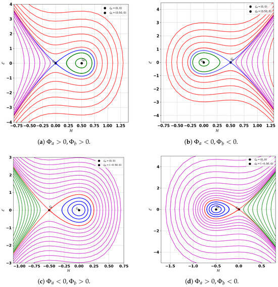  Figure 7. Examining global phase portraits of the unperturbed system (86) across distinct ${\mathrm{\Phi }}_a$ and ${\mathrm{\Phi }}_b$ conditions.

  2.

  For ${\mathrm{\Phi }}_a<0,{\mathrm{\Phi }}_b<0$, the equilibrium points remain $G_a=(0,0)$ and $G_b=(0.50,0)$, but in this case, $G_b$ is a saddle (unstable), and $G_a$ is a center (stable) [31]. This result is illustrated in Figure 7b.

• If $\mathrm{\Delta }<0$:

  1.

  For ${\mathrm{\Phi }}_a<0,{\mathrm{\Phi }}_b>0$, the equilibrium points remain $G_a=(0,0)$ and $G_b=(-0.50,0)$, but now $G_b$ is a saddle (unstable), and $G_a$ is a center (stable). This result is illustrated in Figure 7c.

  2.

  For ${\mathrm{\Phi }}_a>0,{\mathrm{\Phi }}_b<0$, the equilibrium points are $G_a=(0,0)$ and $G_b=(-0.50,0)$. Here, $G_a$ is a saddle (unstable), while $G_b$ is a center (stable). This result is illustrated in Figure 7d.

8. Chaotic and Quasi-Periodic Behaviors

This section focuses on analyzing the quasi-periodic and chaotic behaviors of the given model after incorporating the periodic term $A\cos \left(\omega t\right)$ into system (86):

$$\left\{\begin{array}{c}\begin{array}{cc}\hfill & {\displaystyle \frac{d\mathcal{H}}{d\Psi }}=\mathcal{E},\hfill \\ \hfill & {\displaystyle \frac{d\mathcal{E}}{d\Psi }}={\mathrm{\Phi }}_a\mathcal{H}-{\mathrm{\Phi }}_b{\mathcal{H}}^2+\varsigma cos({\vartheta }_0\Psi ),\hfill \\ \hfill & {\mathrm{\Phi }}_a={\displaystyle \frac{{\mathrm{\Theta }}_1}{\eta {\mathrm{\Theta }}_2^2{p}^2{\varrho }_0}},{\mathrm{\Phi }}_b={\displaystyle \frac{2{\mathrm{\Theta }}_1\mathrm{\Delta }}{\eta {\mathrm{\Theta }}_2^2{p}^2{\varrho }_0}},{\mathrm{\Theta }}_2,p,\eta ,{\varrho }_0\ne 0.\hfill \end{array}\hfill \end{array}\right.$$

(89)

Here, $\varsigma$ represents the amplitude, and ${\vartheta }_0$ denotes the frequency of the external forcing. The resulting system (89) falls under the category of non-autonomous dynamical systems. Now, we discuss methods for chaos detection.

8.1. 2D Phase Portrait Analysis

This study examines the system’s response to varying perturbation intensities and frequencies by analyzing quasi-periodic and chaotic dynamics while keeping the primary parameters, ${\mathrm{\Phi }}_a$ and ${\mathrm{\Phi }}_b$, fixed. Figure 8a–f illustrates the system’s state with trajectory variations based on frequency and intensity. The investigation employs 2D phase-space trajectories and time series plots to reveal the system’s periodic and quasi-periodic behavior. Quasi-periodic behavior is detected through 2D phase portrait analysis using parameters ${\mathrm{\Phi }}_a=0.6$ and ${\mathrm{\Phi }}_b=3.8$ with varying $\varsigma$ and ${\vartheta }_0$ in Equation (89).

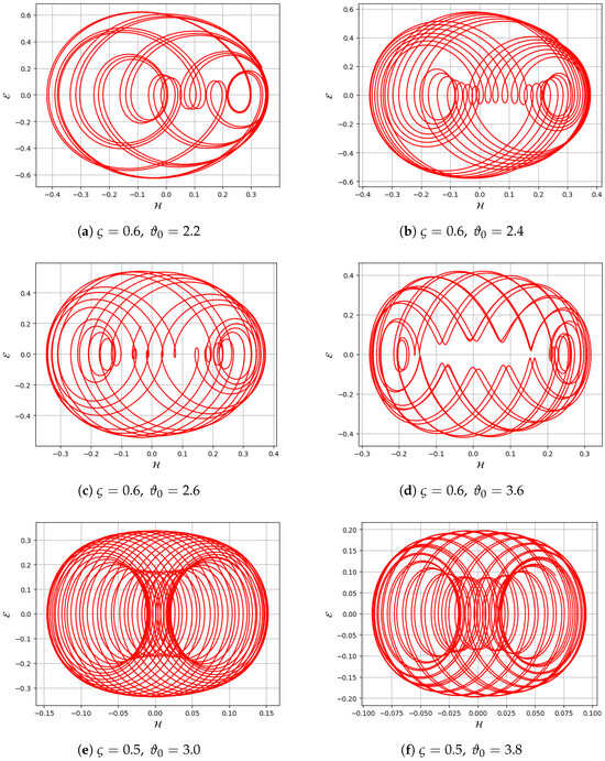
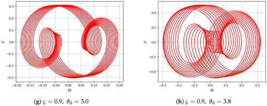
Figure 8. Detection of quasi-periodic behavior in the system through 2D phase portrait with parameters ${\mathrm{\Phi }}_a=0.6$ and ${\mathrm{\Phi }}_b=3.8$, considering different values of $\varsigma$ and ${\vartheta }_0$ in Equation (89).

8.2. Poincare Map Analysis

In this subsection, the chaotic characteristics of the proposed system are investigated using the poincare map analysis, as shown in Figure 9. The poincare map serves as a powerful method to reveal the periodic, quasi-periodic, or chaotic nature of a system by depicting discrete points in its phase space. Quasi-periodic behavior is detected through Poincare map analysis using parameters ${\mathrm{\Phi }}_a=0.6$ and ${\mathrm{\Phi }}_b=3.8$, with varying $\varsigma$ and ${\vartheta }_0$ in Equation (89).

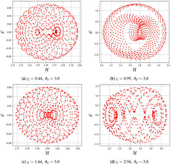
Figure 9. Detection of quasi-periodic behavior in the system through poincare with parameters ${\mathrm{\Phi }}_a=0.6$ and ${\mathrm{\Phi }}_b=3.8$, considering different values of $\varsigma$ and ${\vartheta }_0$ in Equation (89).

8.3. Time Series Analysis

This method is the simplest and relies on visual aids. It examines the system’s state variables, classifying the behavior as chaotic if they exhibit erratic or unpredictable patterns. Otherwise, it is considered non-chaotic, encompassing fixed-point, periodic, and quasi-periodic behaviors. Figure 10 presents the time series of periodic behaviors for system (89) using $\varsigma =0.6$ and ${\vartheta }_0=3.8$, with ${\mathrm{\Phi }}_a>0$, ${\mathrm{\Phi }}_b<0$.

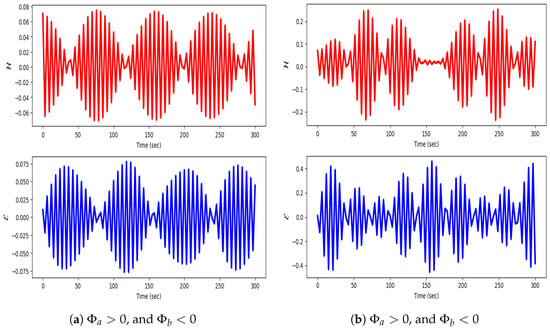
Figure 10. Detection of quasi-periodic behavior in the system using time analysis with parameters $\varsigma =0.6$, and ${\vartheta }_0=3.8$, in Equation (89).

8.4. Bifurcation Diagram

In this subsection, the quasi-periodic behavior of the proposed system is identified through the analysis of the bifurcation diagram, as shown in Figure 11. The bifurcation diagram provides a clear visualization of how the qualitative dynamics of the system evolve as the bifurcation parameter $\left(\varsigma \right)$ varies. Initially, for small values of $\left(\varsigma \right)$, the system exhibits stable and regular motion, indicated by a single smooth branch. However, as $\left(\varsigma \right)$ increases, a sequence of bifurcations emerges, leading to period-doubling phenomena and eventually transitioning into a chaotic regime characterized by densely scattered points. The pronounced dispersion of points at higher $\left(\varsigma \right)$ values distinctly signifies the onset of chaotic behavior.

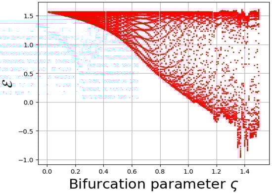
Figure 11. Detection of quasi-periodic behavior in the system using bifurcation diagram with parameters ${\vartheta }_0=3.8$, in Equation (89).

8.5. Lyapunov Exponents

In this subsection, the chaotic nature of the proposed system is examined using Lyapunov exponent analysis, as illustrated in Figure 12 using the values of $\varsigma =0.6$ and ${\vartheta }_0=3.8$, with ${\mathrm{\Phi }}_a>0$, ${\mathrm{\Phi }}_b<0$. The Lyapunov exponents serve as key indicators of chaos, quantifying the average rates at which nearby trajectories in the phase space diverge or converge over time.

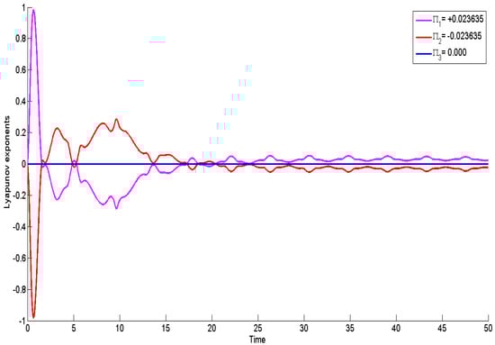
Figure 12. Detection of quasi-periodic behavior in the system using lyapunov exponents with parameters $\varsigma =0.6$ and ${\vartheta }_0=3.8$, with ${\mathrm{\Phi }}_a>0$, ${\mathrm{\Phi }}_b<0$, in Equation (89).

8.6. Fractal Dimension

Fractal dimension measures the complexity of an attractor, with non-integer values indicating chaos. Higher FD suggests increased unpredictability and self-similarity. It helps distinguish between regular and chaotic motion. Figure 13a presents the fractal dimension of periodic behaviors for system (89) using $\varsigma =0.6$ and ${\vartheta }_0=3.8$, with ${\mathrm{\Phi }}_a>0$, ${\mathrm{\Phi }}_b<0$.

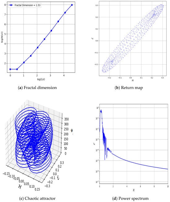
Figure 13. Detection of quasi-periodic behavior in the system using different tools with parameters $\varsigma =0.6$, ${\vartheta }_0=3.8$, ${\mathrm{\Phi }}_a>0$, and ${\mathrm{\Phi }}_b<0$ in Equation (89).

8.7. Return Map

Plots successive values of a variable to reveal patterns; scattered points suggest chaotic behavior. Identifying irregular distributions in return maps helps detect sensitive dependence on initial conditions. Figure 13b presents the return map of periodic behaviors for system (89) using $\varsigma =0.6$ and ${\vartheta }_0=3.8$, with ${\mathrm{\Phi }}_a>0$, ${\mathrm{\Phi }}_b<0$.

8.8. Chaotic Attractor

A trajectory in phase space showing sensitivity to initial conditions, confirming chaos. The attractor’s shape and structure provide insight into the system’s long-term behavior. Figure 13c presents the chaotic attractor of periodic behaviors for system (89) using $\varsigma =0.6$ and ${\vartheta }_0=3.8$, with ${\mathrm{\Phi }}_a>0$, ${\mathrm{\Phi }}_b<0$.

8.9. Power Spectrum

Analyzes frequency components; a broad, continuous spectrum signifies chaotic dynamics. Sharp peaks indicate periodicity, whereas a dense spectrum suggests a transition to chaos. Figure 13d presents the power spectrum of periodic behaviors for system (89) using $\varsigma =0.6$ and ${\vartheta }_0=3.8$, with ${\mathrm{\Phi }}_a>0$, ${\mathrm{\Phi }}_b<0$.

9. Multistability Analysis

Multistability refers to the coexistence of multiple solutions within a dynamical system under specific physical parameters and initial conditions [32,33]. This section examines the perturbed system (86) with an external forcing term $A_0\cos \left(\eta t\right)$ to explore its multistable behavior. Phase graphs and corresponding time series plots are utilized to analyze these dynamics in system (89). Figure 14a depicts quasi-periodic behavior for initial conditions $(\mathcal{H},\mathcal{E})=(0.22,0.01)$ (blue) and periodic behavior for $(\mathcal{H},\mathcal{E})=(0.24,0.01)$ (red) with $\varsigma =0.6$ and ${\vartheta }_0=2.4$. Figure 14b shows quasi-periodic behavior for $(\mathcal{H},\mathcal{E})=(0.22,0.01)$ (blue) and periodic behavior for $(\mathcal{H},\mathcal{E})=(0.23,0.01)$ (red) under the same parameters. Figure 14c presents quasi-periodic behavior for $(\mathcal{H},\mathcal{E})=(0.22,0.01)$ (blue) and periodic behavior for $(\mathcal{H},\mathcal{E})=(0.25,0.01)$ (red). Figure 14d illustrates quasi-periodic behavior for $(\mathcal{H},\mathcal{E})=(0.22,0.01)$ (blue) and periodic behavior for $(\mathcal{H},\mathcal{E})=(0.26,0.01)$ (red). Overall, the observations confirm that the system exhibits quasi-periodic behavior.

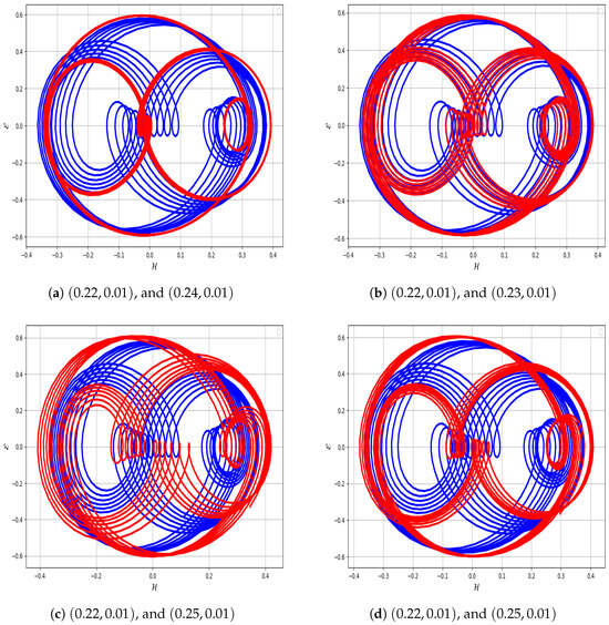
Figure 14. Detection of quasi-periodic behavior in the system using multistability analysis with parameters $\varsigma =0.6$, ${\vartheta }_0=2.4$, ${\mathrm{\Phi }}_a>0$, and ${\mathrm{\Phi }}_b<0$ in Equation (89).

10. Comparison with Existing Literature

The table below (Table 1) outlines the main distinctions between this study and that of Khater et al. [22] on the Equation (1), underscoring the novel aspects of the present work in terms of methodology, solution analysis, and investigation of dynamical behaviors.

Table 1. Comparison between the current study and Khater et al. [22].

Current Study	Khater et al.’s Work [22]
Investigates the Lie symmetry structure of the model to reveal invariant properties.	No analysis based on Lie symmetry.
Derives and verifies conservation laws to identify conserved physical quantities.	Does not explore conservation laws.
Employs the multivariate generalized exponential rational integral function method for obtaining diverse soliton solutions.	Utilizes the extended simple equation, homotopy perturbation and adomian decomposition for soliton solutions.
Performs comprehensive Hamiltonian and bifurcation analyses to understand system stability and dynamics.	Lacks Hamiltonian and bifurcation evaluations.
Conducts chaos detection through computational tools such as phase portraits, Lyapunov exponents, and bifurcation diagrams.	No investigation of chaos analysis.
${\mathcal{J}}_{12}(\alpha ,\mathfrak{T})={\mathcal{V}}_0+{\displaystyle \frac{{\mathcal{V}}_1}{2}}{e}^{-{\displaystyle \frac{\Psi }{2}}}+{\displaystyle \frac{{\mathcal{V}}_1}{2}}{e}^{{\displaystyle \frac{\Psi }{2}}}+e^{-\Psi }{\mathcal{V}}_2+e^{\Psi }{\mathcal{V}}_2-$$2{\mathcal{V}}_2+{\displaystyle \frac{2e^{\frac{\Psi }{2}}{\mathcal{G}}_1}{e^{\Psi }+1}}.$	$J(\alpha ,\mathfrak{T})={\displaystyle \frac{12\sqrt{-\alpha {\mu }^2{a}^3(-b^2)}\tanh \left(\zeta \sqrt{-\alpha \mu }-\frac{\log \left(v\right)}{2}\right)}{a{b}^2}}-{\displaystyle \frac{\sqrt{{\alpha }^6{b}^2{\mu }^2}}{a^2{b}^2}}-{\displaystyle \frac{6\alpha \mu {\mathrm{sech}}^2\left(\zeta \sqrt{-\alpha \mu }-\frac{\log \left(v\right)}{2}\right)}{b}}$
${\mathcal{J}}_5(\alpha ,\mathfrak{T})={\displaystyle \frac{{\mathcal{V}}_2}{4}}{\left(e^{i(\alpha -\eta \mathfrak{T})}+e^{i(\eta \mathfrak{T}-\alpha )}\right)}^2+{\displaystyle \frac{4{\mathcal{G}}_2{e}^{2i(\eta \mathfrak{T}+\alpha )}}{{\left(e^{2i\eta \mathfrak{T}}+e^{2i\alpha }\right)}^2}}+{\mathcal{V}}_0.$	$J(\alpha ,\mathfrak{T})={\displaystyle \frac{3\sqrt{b^2{({\lambda }^2-4\mu )}^2}+\sqrt{b^2({\lambda }^2-4\mu )}}{b^2}}[\left(\lambda \right.$
	$-{\displaystyle \frac{{\displaystyle \frac{4\mu }{\lambda -\sqrt{{\lambda }^2-4\mu }}}\tanh \left(\frac{1}{2}\sqrt{{\lambda }^2-4\mu }(\xi +\theta )\right)}{2b\mu ({\lambda }^2-4\mu )}})$
	$+\left(\lambda \cosh \left(\frac{1}{2}\sqrt{{\lambda }^2-4\mu }(\xi +\theta )\right)-\sqrt{{\lambda }^2-4\mu }\right.$
	${\left.\sinh \left(\frac{1}{2}\sqrt{{\lambda }^2-4\mu }(\xi +\theta )\right)\right)}^2]$

11. Conclusions

This study focuses on the investigation of a microtubule equation, employing Lie symmetry analysis to identify Lie point symmetries based on the invariance criterion of Lie groups. Through similarity reduction, the governing PDE is systematically reduced to an ODE. The MGERIF method generates diverse soliton profiles by tuning parameters, with 3D and contour plots illustrating the real, imaginary, and modulus parts of ${\mathcal{J}}_1,{\mathcal{J}}_2,{\mathcal{J}}_4,{\mathcal{J}}_5,$ and ${\mathcal{J}}_6$. In addition, a qualitative dynamical study is performed through bifurcation and chaos analysis. Utilizing a Galilean transformation, the system is reformulated into first-order differential equations, followed by bifurcation analysis under varying ${\mathrm{\Phi }}_a$ and ${\mathrm{\Phi }}_b$, as shown in Figure 7. Upon introducing an external periodic force $\varsigma \cos \left({\vartheta }_0\mathfrak{T}\right)$, the system demonstrates both quasi-periodic and chaotic behavior. This complex behavior is examined using tools such as phase portrait, time analysis, fractal dimension, return map, chaotic attractor, power spectrum as presented in Figure 8, Figure 9, Figure 10, Figure 11, Figure 12, Figure 13 and Figure 14. The multistability of the system is further explored by varying initial conditions, indicating low sensitivity to perturbations, as shown in Figure 14. Conservation laws are also derived, offering deeper insight into the mathematical structure of the model.

Future directions: In future research, this study can be extended to (n + 1)-dimensional cases to explore more complex physical phenomena. Moreover, various analytical and numerical techniques can be employed to obtain broader classes of solutions and enhance the understanding of nonlinear dynamics. These methods include the variational iteration method, adomian decomposition method (ADM), perturbation techniques, lump and breather solutions, neural network-based schemes, and physics-informed neural networks. Such extensions may provide deeper insights into the stability, bifurcation behavior, and potential applications of the system in real-world scenarios.

References

- Kumar, S.; Niwas, M. Exact closed-form solutions and dynamics of solitons for a (2+1)-dimensional universal hierarchy equation via Lie approach. Pramana 2021, 95, 195. [Google Scholar] [CrossRef]
- Younas, U.; Hussain, E.; Muhammad, J.; Sharaf, M.; Meligy, M.E. Chaotic Structure, Sensitivity Analysis and Dynamics of Solitons to the Nonlinear Fractional Longitudinal Wave Equation. Int. J. Theor. Phys. 2025, 64, 42. [Google Scholar] [CrossRef]
- Hussain, E.; Tedjani, A.H.; Farooq, K.; Beenish. Modeling and Exploration of Localized Wave Phenomena in Optical Fibers Using the Generalized Kundu–Eckhaus Equation for Femtosecond Pulse Transmission. Axioms 2025, 14, 513. [Google Scholar] [CrossRef]
- Kopçasız, B.; Yaşar, E. Inquisition of optical soliton structure and qualitative analysis for the complex-coupled Kuralay system. Mod. Phys. Lett. B 2025, 39, 2450512. [Google Scholar] [CrossRef]
- Kopçasız, B. Unveiling new exact solutions of the complex-coupled Kuralay system using the generalized Riccati equation mapping method. J. Math. Sci. Model. 2024, 7, 146–156. [Google Scholar] [CrossRef]
- Tipu, G.H.; Faridi, W.A.; Yao, F.; Garayev, M. Uncovering nonlinear dynamics in shallow water: An analytic approach to the (1+1)-dimensional Estevez–Mansfield–Clarkson equation. J. Ocean. Eng. Mar. Energy 2025, 11, 799–818. [Google Scholar] [CrossRef]
- Xu, J.; Fan, L.; Chen, C.; Lu, G.; Li, B.; Tu, T. Study on fuel injection stability improvement in marine low-speed dual-fuel engines. Appl. Therm. Eng. 2024, 253, 123729. [Google Scholar] [CrossRef]
- Zinat, N.; Hussain, A.; Kara, A.H.; Zaman, F.D. On the analysis and integrability of the time-fractional stochastic potential-KdV equation. Quaest. Math. 2025, 48, 909–928. [Google Scholar] [CrossRef]
- Yin, X.; Lai, Y.; Zhang, X.; Zhang, T.; Tian, J.; Du, Y.; Gao, J. Targeted sonodynamic therapy platform for holistic integrative Helicobacter pylori therapy. Adv. Sci. 2025, 12, 2408583. [Google Scholar] [CrossRef]
- Fang, Q.; Sun, Q.; Ge, J.; Wang, H.; Qi, J. Multidimensional Engineering of Nanoconfined Catalysis: Frontiers in Carbon-Based Energy Conversion and Utilization. Catalysts 2025, 15, 477. [Google Scholar] [CrossRef]
- Liu, W.; Gao, Z.; Wei, Z.; Zhang, L.; Guo, G.; Mumtaz, S. Compensator-Based Fixed-Time Prescribed Performance Control of Vehicular Platoon with Input Nonlinearities: A Performance Boundary Self-Adjusting Approach. IEEE Trans. Intell. Transp. Syst. 2025, 26, 14823–14837. [Google Scholar] [CrossRef]
- Khater, M.M.; Mohamed, M.S.; Attia, R.A. On semi analytical and numerical simulations for a mathematical biological model; the time-fractional nonlinear Kolmogorov–Petrovskii–Piskunov (KPP) equation. Chaos Solitons Fractals 2021, 144, 110676. [Google Scholar] [CrossRef]
- Khater, M.M.; Ahmed, A.E.S.; El-Shorbagy, M.A. Abundant stable computational solutions of Atangana–Baleanu fractional nonlinear HIV-1 infection of CD4+ T-cells of immunodeficiency syndrome. Results Phys. 2021, 22, 103890. [Google Scholar] [CrossRef]
- Khater, M.M.; Nisar, K.S.; Mohamed, M.S. Numerical investigation for the fractional nonlinear space-time telegraph equation via the trigonometric Quintic B-spline scheme. Math. Methods Appl. Sci. 2021, 44, 4598–4606. [Google Scholar] [CrossRef]
- Khater, M.M.; Nofal, T.A.; Abu-Zinadah, H.; Lotayif, M.S.; Lu, D. Novel computational and accurate numerical solutions of the modified Benjamin–Bona–Mahony (BBM) equation arising in the optical illusions field. Alex. Eng. J. 2021, 60, 1797–1806. [Google Scholar] [CrossRef]
- Liu, Z.; Liu, B.; Chen, L.; Tian, F.; Xu, J.; Liu, J.; Zhu, B. Effect of lateral stress and loading paths on direct shear strength and fracture of granite under true triaxial stress state by a self-developed device. Eng. Fract. Mech. 2025, 318, 110952. [Google Scholar] [CrossRef]
- Gao, Z.; Wei, Z.; Liu, W.; Zhang, L.; Wen, S.; Guo, G. Global prescribed performance control for 2-D plane vehicular platoons with small overshoot: A fixed-time composite sliding mode control approach. IEEE Trans. Intell. Transp. Syst. 2025, 26, 18789–18804. [Google Scholar] [CrossRef]
- Zhang, Y.; Jiang, C.; Li, M.; Qi, Z.; Yang, X.; Lin, Y.; Cao, S. A review on curve edge based architectures under lateral loads. Thin-Walled Struct. 2025, 217, 113849. [Google Scholar] [CrossRef]
- Ma, C.; Huang, S.; Li, M.; He, J.; Totis, G.; Hua, C.; Weng, S. Highly efficient heat dissipation method of grooved heat pipe for thermal behavior regulation for spindle system working in low rotational speed. Int. Commun. Heat Mass Transf. 2025, 169, 109575. [Google Scholar] [CrossRef]
- Ma, C.; Li, M.; Liu, J.; Li, M.; He, J.; Totis, G.; Weng, S. High-efficiency topology optimization method for thermal-fluid problems in cooling jacket of high-speed motorized spindle. Int. Commun. Heat Mass Transf. 2025, 169, 109533. [Google Scholar] [CrossRef]
- Zhang, W.; Zhang, A.; Zhang, L.; Cui, R.; Lv, B.; Xiao, Z.; Xu, X. Light modulated magnetism and spin–orbit torque in a heavy metal/ferromagnet heterostructure based on van der Waals-layered ferroelectric materials. Appl. Phys. Lett. 2023, 123, 092406. [Google Scholar] [CrossRef]
- Khater, M.M.; Lu, D.; Inc, M. Diverse novel solutions for the ionic current using the microtubule equation based on two recent computational schemes. J. Comput. Electron. 2021, 20, 2604–2613. [Google Scholar] [CrossRef]
- Khan, A.; Alshammari, F.S.; Yasin, S. Exact Solitary Wave Solutions and Sensitivity Analysis of the Fractional (3+1) D KdV–ZK Equation. Fractal Fract. 2025, 9, 476. [Google Scholar] [CrossRef]
- San, S.; Alshammari, F.S. Analytical and Dynamical Study of Solitary Waves in a Fractional Magneto-Electro-Elastic System. Fractal Fract. 2025, 9, 309. [Google Scholar] [CrossRef]
- Khan, M.I.; Ali, U. Novel Exact Solutions of a Higher-Dimensional Complex KdV System with Conformable Derivative Using the Generalized Expansion Method. J. Math. Anal. Model. 2025, 6, 1–25. [Google Scholar] [CrossRef]
- Zhang, H.; Chang, Y.; Xu, Y.; Liu, C.; Xiao, X.; Li, J.; Guo, H. Design and fabrication of a chalcogenide hollow-core anti-resonant fiber for mid-infrared applications. Opt. Express 2023, 31, 7659–7670. [Google Scholar] [CrossRef] [PubMed]
- Chen, Z.; Li, B.; Wang, B. Robust stability design for inverters using phase lag in proportional-resonant controllers. IEEE Trans. Ind. Electron. 2025, 72, 2655–2668. [Google Scholar] [CrossRef]
- Zhao, Q.; Zhang, H.; Xia, Y.; Chen, Q.; Ye, Y. Equivalence relation analysis and design of repetitive controllers and multiple quasi-resonant controllers for single-phase inverters. IEEE J. Emerg. Sel. Top. Power Electron. 2025, 13, 3338–3349. [Google Scholar] [CrossRef]
- Jing, H.; Lin, Q.; Liu, M.; Liu, H. Electromechanical braking systems and control technology: A survey and practice. Proc. Inst. Mech. Eng. Part J. Automob. Eng. 2025, 239, 4551–4573. [Google Scholar] [CrossRef]
- Hale, J.K.; Koçak, H. Dynamics and Bifurcations; Springer Science & Business Media: Berlin/Heidelberg, Germany, 2012; Volume 3. [Google Scholar]
- Sun, L.; Li, M.; Song, Z.; Fu, T.; Hao, X.; Li, Y.; Sotskov, Y. An Integrated MILP Model for Scheduling of Steelmaking-Continuous Casting with Cranes. IEEE Robot. Autom. Lett. 2025, 10, 10426–10433. [Google Scholar] [CrossRef]
- Gao, S.; Ding, S.; Ho-Ching Iu, H.; Erkan, U.; Toktas, A.; Simsek, C.; Mou, J. A three-dimensional memristor-based hyperchaotic map for pseudorandom number generation and multi-image encryption. Chaos Interdiscip. J. Nonlinear Sci. 2025, 35, 073105. [Google Scholar] [CrossRef]
- Mouhsine, H.; Mokni, K.; Ch-Chaoui, M. Exploring multi-parameter bifurcations and immigrationdriven dynamics in a discrete-time Bazykin–Berezovskaya prey–predator model. Nonlinear Dyn. 2025, 113, 34101–34131. [Google Scholar] [CrossRef]
Disclaimer/Publisher’s Note: The statements, opinions and data contained in all publications are solely those of the individual author(s) and contributor(s) and not of MDPI and/or the editor(s). MDPI and/or the editor(s) disclaim responsibility for any injury to people or property resulting from any ideas, methods, instructions or products referred to in the content. |
© 2025 by the authors. Licensee MDPI, Basel, Switzerland. This article is an open access article distributed under the terms and conditions of the Creative Commons Attribution (CC BY) license (https://creativecommons.org/licenses/by/4.0/).