Label-Driven Optimization of Trading Models Across Indices and Stocks: Maximizing Percentage Profitability

Abstract

Short-term trading presents a high-dimensional prediction problem, where the profitability of trading signals depends not only on model accuracy but also on how financial labels are defined and aligned with market dynamics. Traditional approaches often apply uniform modeling choices across assets, overlooking the asset-specific nature of volatility, liquidity, and market response. In this work, we introduce a structured, label-aware machine learning pipeline aimed at maximizing short-term trading profitability across four major benchmarks: S&P 500 (SPX), NASDAQ-100 (NDX), Dow Jones Industrial Average (DJI), and the Tadāwul All-Share Index (TASI and twelve of their most actively traded constituents). Our solution systematically evaluates all combinations of six model types (logistic regression, support vector machines, random forest, XGBoost, 1-D CNN, and LSTM), eight look-ahead labeling windows (3 to 10 days), and four feature subset sizes (44, 26, 17, 8 variables) derived through Random Forest permutation-importance ranking. Backtests are conducted using realistic long/flat simulations with zero commission, optimizing for Percentage Profit and Profit Factor on a 2005–2021 train/2022–2024 test split. The central contribution of the framework is a labeling-aware search mechanism that assigns to each asset its optimal combination of model type, look-ahead horizon, and feature subset based on out-of-sample profitability. Empirical results show that while XGBoost performs best on average, CNN and LSTM achieve standout gains on highly volatile tech stocks. The optimal look-ahead window varies by market from 3-day signals on liquid U.S. shares to 6–10-day signals on the less-liquid TASI universe. This joint model–label–feature optimization avoids one-size-fits-all assumptions and yields transferable configurations that cut grid-search cost when deploying from index level to constituent stocks, improving data efficiency, enhancing robustness, and supporting more adaptive portfolio construction in short-horizon trading strategies.

1. Introduction

The field of financial time series forecasting represents a challenging yet critical aspect of quantitative finance, where the accurate prediction of asset prices, trends, and returns is fundamental to informed decision-making and portfolio management [1,2]. Financial markets are volatile, non-stationary, and prone to structural shifts, posing distinct challenges for traditional statistical models [3]. Unlike the relatively stable patterns seen in time series data from other disciplines, financial data exhibit characteristics such as heavy-tailed return distributions, volatility clustering, and abrupt shifts driven by external events like financial crises, political disruptions, or shifts in market sentiment [4]. These properties make financial forecasting particularly difficult, with classical models based on Gaussian assumptions often proving inadequate. Furthermore, the emphasis in finance on practical metrics such as profit, drawdown, and turnover adds complexity, making conventional machine learning error scores less relevant for evaluation [5].

Machine learning has gained increased prominence in financial forecasting research and practice, driven by the need to move beyond conventional models and improve robustness and predictive accuracy [6,7]. However, a critical limitation of machine learning lies in its dependence on high-quality datasets, carefully selected features, and thoughtfully designed labels [8]. The high-dimensional nature of financial time series means that they contains a wide range of indicators, not all of which are relevant for predictive modeling [9]. While many studies employ feature sets with hundreds of indicators, they often neglect to address the risks of noise and overfitting. Moreover, conventional labeling methods such as predicting daily price changes or five-day returns frequently fail to account for the instability and trading volume dynamics unique to different financial instruments [10]. Addressing these challenges is essential to ensure that theoretical models generalize well to unseen data and perform reliably in real-world scenarios.

Previous efforts have often relied on singular models or fixed look-ahead horizons applied uniformly across all assets, without accounting for the distinct characteristics of financial data specific to each asset [11]. Many studies employ models such as Long Short-Term Memory (LSTM) networks or Convolutional Neural Networks (CNN), yet they typically overlook the fact that these architectures do not guarantee consistent performance across different regimes or asset types [12,13]. Financial market volatility is asset-dependent, and the optimal predictive horizon or look-ahead window is highly specific to the asset class [14]. For instance, highly liquid markets generally benefit from shorter prediction horizons, whereas less liquid assets may yield better performance with longer look-ahead [15]. As a result, models that ignore these distinctions often perform well only under narrow market conditions and fail when applied to different environments or asset classes.

Furthermore, the feature selection process often introduces irrelevant or redundant variables, adding unnecessary complexity and potentially increasing look-ahead bias [16]. As a result, many models fail to isolate the key factors driving market behavior, thereby undermines their predictive effectiveness. Identifying truly informative features remains a significant challenge, and this difficulty is compounded by the need to design labels that accurately reflect the underlying dynamics of financial markets [17]. Improving the performance of financial forecasting models thus requires a more careful and adaptive approach to both feature selection and label construction.

This study aims to address these challenges by proposing a comprehensive, labeling-aware machine learning pipeline that adapts to the unique characteristics of each asset. The framework jointly optimizes the key elements of model selection, feature selection, and label definition, taking into account the dynamic and market-specific nature of financial data. By treating the look-ahead window and feature subset as hyper-parameters to be tuned for each asset, we ensure that the model is better aligned with the asset’s liquidity, volatility, and trading behavior. Furthermore, by using a range of machine learning models such as tree ensembles (XGBoost, RF), linear models (logistic regression, SVM), and deep learning models (1-D CNN, LSTM) we explore how different approaches can be combined with optimized labels and features to improve model performance.

This study presents several key contributions to the field of financial time series forecasting:

i.

Stock-Specific Label Tuning: We introduce the concept of dynamically tuning the look-ahead window for each asset. Our research shows that the optimal look-ahead window varies across different assets, with liquid U.S. stocks requiring shorter windows (3 days) and less-liquid markets like TASI benefiting from longer windows (6–10 days). This demonstrates the importance of considering market latency when designing labels.

ii.

Compact Feature Discovery: Using Random Forest’s permutation importance, we rank engineered factors and apply compression techniques to reduce the feature set. By selecting the most 85 informative features, we reduce overfitting through k-fold cross-validation while ensuring that essential signals related to momentum, volatility, and order flow are preserved.

iii.

Model–Label–Feature Optimization: The study evaluates a diverse set of machine learning models, including tree ensembles, linear models, and deep neural networks, in combination with optimized labels and feature sets. This comprehensive approach enables the identification of the best model-label-feature combination for each asset, ensuring that the model is well-suited to the specific characteristics of the asset.

iv.

Transferable Configurations: One of the key advantages of this framework is its ability to provide adaptable configurations across different assets. We show that the configuration that maximizes performance at the index level often also improves the performance of individual constituents, thereby reducing the need for time-consuming grid searches and enabling efficient deployment in real-time trading systems.

2. Literature Review

Recent advances in financial forecasting increasingly emphasize the critical role of label construction and feature selection in determining model effectiveness. Since financial time series are inherently noisy and non-stationary, how labels are defined particularly with respect to look-ahead windows and trend thresholds significantly impacts predictive accuracy and trading performance. Likewise, the selection of informative features from a high-dimensional input space remains essential, because such useless activities may obscure real market trends. Researchers have considered classic and state of the art methods to address these issues, including the development of time sensitive weighting mechanisms, flexible marking methods, and feature selection systems suitable to model and market dynamics.

2.1. Feature Engineering and Selection

Recent studies have advanced feature engineering techniques to enhance the predictive performance of financial models by integrating a diverse set of data types and selection strategies. Vaidynathan et al. [18] developed a reliable feature set for IPO performance forecasting, employing numerical variables such as IPO price and financial gains/losses as well as textual cues. The research utilizes BERT-based contextual embedding, sentiment analysis, and normalized Google Trends interest trends to measure the degree of attention by the public. In order to overcome missing data issues, Vaidynathan et al. use Boolean indicators and set the missing data to zero. This multimodal approach results in a comprehensive and interpretable input space, further augmented through SHAP value analysis for model explanation. Similarly, Pabuccu and Barbu [19] explore over 1000 technical indicators for financial time-series forecasting and propose Feature Selection with Annealing (FSA) as a robust method for identifying high-value features. FSA outperforms traditional techniques like Lasso and Boruta, highlighting its utility in refining noisy, high-dimensional financial data for both regression and classification tasks.

Feature selection strategies have also evolved to account for temporal and structural heterogeneity across financial domains. Kim et al. [20] introduce a Dynamic Feature Selection System (DFSS) that utilizes 16 algorithms spanning embedded and ensemble types to identify time-sensitive and industry-specific feature subsets for stock price prediction across 10 major sectors in South Korea. This framework allows for adaptive modeling that reflects changing market dynamics, improving both interpretability and model performance.

Paramita and Winata [21] carry out a comparative analysis of PCA, Information Gain, and Recursive Feature Elimination (RFE), concluding that RFE outperforms both PCA and Information Gain for stock prediction due to the iterative elimination of irrelevant features. Finally, Han et al. [22] propose a new perspective on feature engineering by suggesting Selective Genetic Algorithm (SGA) that denoises price signals and better aligns features with trading actions. By combining these results, we observe that feature engineering is critical to increasing the trustworthiness, clarity, and economic potential of financial machine learning systems.

2.2. Machine Learning Models

In the last decade, there has been the increased utilization of the machine learning and deep learning models in stock market prediction owing to the complexity and non-linearity of the financial data. Wang et al. [23], propose a hierarchical adaptive temporal-relational network (HATR) to capture the short- and long-term patterns in the trading sequences of stocks through dilated causal convolutions and gated paths. A multi-graph interaction module provides efficient domain knowledge including adaptive learning with superior performance in a variety of datasets with a dual attention mechanism improving temporal sensitivity. Citing the same sentiment, Al-Khasawneh et al. [24] use Long Short-Term Memory (LSTM) networks to predict the Pakistan Stock Exchange index based on their ability to model sequential relationships in time series data. Shen and Shafiq [25] also build a system of deep learning that is specifically designed for Chinese stock market, operating with a number of adjusted architectures, complete with exhaustive pre-processing and feature engineering to attain high accuracies in prediction for different periods of anticipation.

On the other hand, the traditional machine learning models are still applicable, especially in cases where structures of data or interpretability of models are preferred. Kumar et al. [26] compare 4 supervised learning algorithms: SVM, Random Forest, KNN and Naive Bayes, and find Random Forest to be the most appropriate for large dataset followed by Naive Bayes for smaller dataset. Yin et al. [5] extend Random Forest by coming up with the D-RF-RS method that combines the use of exponential smoothing, technical indicator extraction, decision tree-based feature selection and hyper-parameter tuning through random search to improve the accuracy and robustness of the model. Chen et al. [27] apply LightGBM in the context of a trading strategy that involves risk constraints through the usage of Conditional Value at Risk (CVaR). LightGBM’s capability to model, non-linear relationship and process sparse, high dimensional data through mutual exclusive feature bundling results in successful stock prediction and risk conscious portfolio formation. Together, these studies paint the adaptability and stay of both deep and traditional machine learning models for financial forecasting.

2.3. Labeling Look Ahead Windows and Optimization Strategies

Several studies have focused on enhancing labeling methods to improve the accuracy and robustness of stock price trend predictions. Ma et al. [28] explored the use of self-supervised learning techniques, particularly denoising autoencoders, to generate more accurate labels by reducing noise exposure in financial time series. This method delivered significant advances in the model’s performance for the small and the large dataset, indicating the optimized label generation can play an important role in enhancing market trend prediction. Similarly, a noise model was introduced by Kovacevic et al., [29] to measure the robustness of trend labeling algorithms with an intention to optimize labels for classification algorithms. Their model enables evaluating effectiveness of trend labeling without classifier training, which eventually will enhance the classifier performance in the task of determining the price of an asset.

Zhao et al., [30] indicated the importance of time-series data in trend prediction and introduced a time-weighted function which assigns weights to the data according to its temporal relationship with the target data. Such an approach increased the predictive precision of the Long Short-Term Memory (LSTM) network, reaching 83.91% of the accuracy rate in predictions for CSI 300 index. Bounid et al. [31] also had contributed by incorporating the cutting-edge methods of the preprocessing of the financial data, which confirmed that the techniques enhance the compliance of the machine learning models with the actual market conditions. Finally, Saberi et al. [32] proposed the Dynamic Threshold Breakout (DTB) labeling system which uses price percentage difference over certain periods to label data. This method overcame the inefficiencies of conventional labeling, causing great trading performance in various markets when connected with LightGBM, increasing precision, ROI, and other metrics of trading.

3. Dataset and Feature Engineering

This study examines the viability of short-term trading strategies built on the principles of machine learning for a representative set of indices and its constituents. The selection includes major U.S. markets and a regional one from the Middle East region, so that it represents a wide range of asset classes, sectors, and volatility regimes. We create a consistent and high-quality dataset from 2005 to 2024 and calculate comprehensive set of technical features for predictive modeling.

3.1. Instrument Universe

Our research covers four leading indices and twelve representative constituents to represent our broad market coverage and sectoral diversity, respectively. The U.S. indices (S&P 500 (SPX), NASDAQ-100 (NASDAQ), and Dow Jones Industrial Average (DJI)) are complemented with the Tadāwul All-Share Index (TASI), to provide regional exposure from the Saudi market. Each index has the following three liquid constituents, which are selected based on continuity of data and market relevance (Table 1).

Table 1. Instrument universe and sample sizes (2005–2024).

Index	Constituents Analyzed	Raw Bars (2005–2024)
SPX	AAPL, JNJ, XOM	5008
NASDAQ	ADBE, AMZN, NVDA	5008
DJI	IBM, GS, KO	5008
TASI	Al-Rajhi Bank (1120), SABIC (2010), STC (7010)	4732

Daily OHLCV (Open, High, Low, Close, and Volume) data are sourced from the EOD-Historical-Data API for U.S. instruments and from Tadāwul’s public API for Saudi assets. All series are aligned to a common trading calendar and split chronologically into:

• Train: 2005–2021
• Test: 2022–2024

3.2. Constituent Selection and Sample Representativeness

The study focuses on a total of twelve actively traded constituents drawn from four major equity benchmarks: the Dow Jones Industrial Average (DJI), the S&P 500 (SPX), the NASDAQ-100 (NASDAQ), and the Tadāwul All-Share Index (TASI). While this number is small relative to the hundreds of names in these indices, the selection is deliberate and methodologically motivated rather than arbitrary. The objective is to obtain a computationally tractable yet highly informative cross-section that spans a broad spectrum of volatility, liquidity, and sectoral profiles, enabling a clean evaluation of how label design interacts with asset microstructure.

The primary selection criterion is liquidity and data completeness. Each constituent is required to exhibit high and stable trading activity and to have uninterrupted daily OHLCV data from 2005 to 2024. This ensures robust statistical estimation, reliable price discovery, and consistent long-horizon backtesting without survivorship or missing-data distortions.

A second design principle is sectoral and index representativeness. For each index, three constituents are chosen to reflect distinct sectors and trading behaviors, rather than clustering around a single industry. Concretely,

• SPX: AAPL (technology), JNJ (healthcare), XOM (energy);
• NASDAQ-100: ADBE (software), AMZN (e-commerce), NVDA (semiconductors);
• DJI: IBM (technology), GS (financials), KO (consumer staples);
• TASI: Al-Rajhi Bank (banking), SABIC (materials), STC (telecommunications).

This construction yields a miniature but diverse universe that reflects blue-chip, growth, defensive, and cyclical profiles, as well as differences in trading intensity and volatility regimes across U.S. and Saudi markets.

Finally, the sample size is constrained by computational considerations. The proposed framework evaluates, for each instrument, a full grid of model–label–feature combinations comprising 16 instruments × 6 model types × 8 look-ahead horizons × 4 feature subset sizes. This 3000+ configuration space makes it impractical to include all index constituents while still performing exhaustive out-of-sample testing. Restricting the universe to twelve carefully chosen stocks therefore strikes a practical balance: it keeps the grid search exhaustive and reproducible, while still covering a rich diversity of microstructure conditions. In this sense, the subset is small by design but methodologically representative for the labeling-focused questions studied in this paper.

3.3. Feature Engineering

To support predictive modeling, we construct a library of 85 engineered features for each instrument. These features are designed to capture short-term price dynamics, trend strength, volatility regimes, volume anomalies, and contextual trading behavior. All features are computed from daily OHLCV data using fixed lookback windows ranging from 2 to 5 days, unless otherwise specified. To ensure consistency and avoid forward-looking bias, all features are computed in a rolling manner and normalized prior to model training. To maintain comparability across global indices (US and Saudi Arabia) and ensure the full transferability of the predictive framework, we did not incorporate any fundamental, macroeconomic, or sentiment features.

The feature engineering process incorporates a comprehensive set of 85 technical indicators, categorized into five functional groups (Table 2). Each category captures distinct market behaviors relevant to short-term trading, including momentum, trend, volatility, and contextual effects. These features are computed using short rolling windows (typically 2–5 days) and are normalized to ensure comparability across instruments and time. For example, ADX is considered one of the most important indictors related to trend indicators.

Table 2. Technical Indicators by Category.

Category	Indicators Included	#Var
Momentum/Oscillators	%K, %D, Williams %R, RSI, Connors RSI, True Strength Index, Rate-of-Change	40
Trend indicators	ADX, +DI, –DI, MACD line, MACD Signal, MACD Histogram	35
Raw price/volume	Open, High, Low, Close, Volume	5
Volume/Money flow	Money Flow (MF)	5
Total columns in file		85

These features collectively capture a wide range of trading dynamics. Momentum and oscillators identify overbought/oversold conditions, while trend indicators measure directional strength. Volatility and volume features help account for regime changes and liquidity shifts.

All primary indicators were generated using standardized parameter settings consistent with TA-Lib and Trading View conventions.

To significantly enhance the quality of the features and better capture the rate of change and short-term trends within the features themselves, we introduced regression-based derivative features.

For a core subset of indicators, we calculated the slope coefficient (beta) of a simple linear regression over lookback windows ranging from 2 to 5 bars. This resulted in four additional derivative features for each primary indicator in the subset.

The final, high-quality feature set comprises the original OHLCV data, the primary technical indicators, and these regression-based derivatives (e.g., DI+_{2_reg}, RSI_{5_reg}). This novel method of feature engineering provides the model with a more granular and powerful signal regarding the dynamics of the technical indicators, directly impacting the model’s ability to maximize profitability.

To ensure reproducibility and methodological clarity, all technical indicators were computed using their standard Trading View default configurations. A complete table of indicator names, inputs, and parameter configurations is provided in the next Table 3.

Table 3. Full set of technical indicators parameters.

Indicator Name	Abbreviation	Source Input	Window/Period Settings	Additional Parameters
Relative Strength Index	RSI	Close	Length: 14	Smoothing: SMA(14); BB StdDev: 2
Connors RSI	CRSI	N/A	RSI Length: 3	UpDown Length: 2; ROC Length: 100
Moving Average Convergence Divergence	MACD	Close	Fast Length: 12; Slow Length: 26	Signal Smoothing: 9; Type: EMA
Average Directional Index	ADX	N/A	DI Length: 14	ADX Smoothing: 14
Stochastic Oscillator %K	%K	N/A	Period: 14	—
Stochastic Oscillator %D	%D	Close	Fast Period: 21; Slow Period: 55	—
Average True Range Histogram	Hist	N/A	ATR Length: 14	MA Length: 100; Hist MA Length: 1
Money Flow Index	MFI	N/A	Length: 14	—
True Strength Index	TSI	Close	Long Length: 25; Short Length: 13	Signal Length: 13
Williams %R	%R	Close	Length: 14	—
Rate of Change	ROC	Close	Length: 9	—
Signal Moving Average (LuxAlgo)	Signal	Close	Length: 50	—
Signal Moving Average 2 (LuxAlgo)	Signal.1	Close	Length: 25	—

4. Methodology

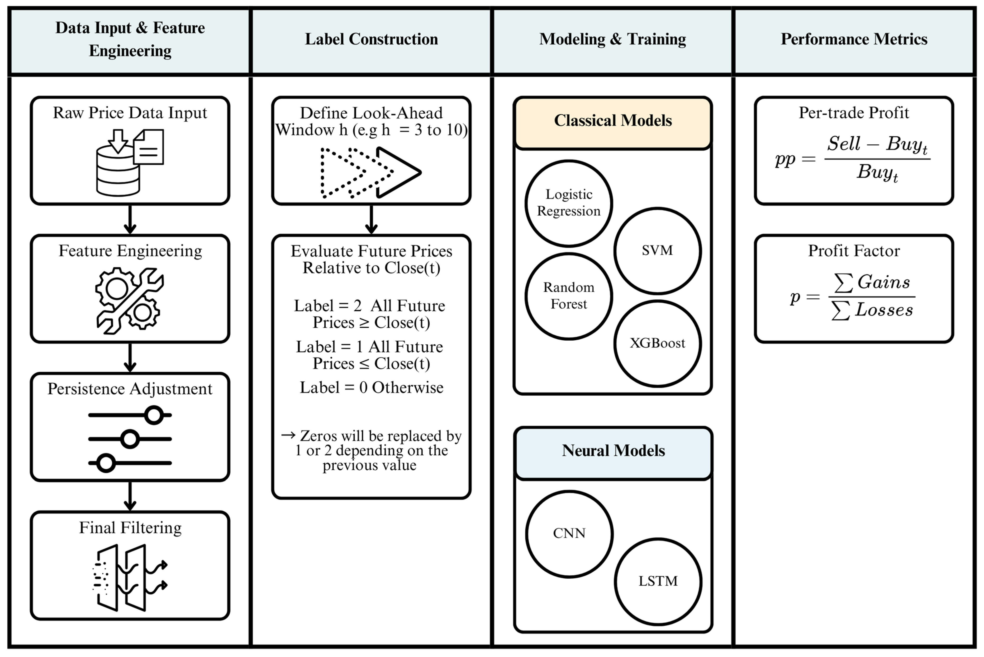
To construct reliable supervised labels for short-term price movement prediction, we adopt a deterministic, rule-based labeling method designed to capture directional momentum over fixed forward-looking intervals. This method, which we refer to as the Monotone-Horizon Signal (MHS), avoids arbitrary thresholds and is grounded entirely in the price path’s monotonic behavior across future periods (Figure 1).

Figure 1. Label-aware machine learning pipeline for optimizing short-term trading strategies.

4.1. Label Construction: Monotone-Horizon Signal (MHS)

At the core of our methodology is the construction of a 3-state label, denoted as MHSh(t) ∈ {2, 1, 0}, where h is the length of the look-ahead horizon in trading days. The label captures whether the closing price maintains a consistent directional relationship with today’s closing price over the next h periods.

For each look-ahead horizon h ∈ {3, 4, … 10}, we define the MHS label in Table 4.

Table 4. Monotone-Horizon Signal Label Definition.

Label Value	Condition	Interpretation
2	∀_i ∈ [1, h],Close(t + i) ≥ Close(t)	A label of ‘2’ signifies that all closing prices from the current time t through the next h1 periods are greater than or equal to today’s closing price, Close(t). This indicates an expectation of a consistently non-decreasing (or upward) movement and can be interpreted as a component of a potential buy signal.
1	∀_i ∈ [1, h],Close(t + i) ≤ Close(t)	A label of ‘1’ is assigned if the condition for ‘2’ is not met, AND all closing prices from the current time t through the next h1 periods are less than or equal to today’s closing price, Close(t). This suggests a consistently non-increasing (or downward) movement, serving as a component of a potential sell signal.
0	Otherwise (i.e., price fluctuates both above and below today’s close in the next h days)	A label of ‘0’ is assigned if neither of the above conditions is met, meaning the price does not maintain a monotonic direction (relative to Close(t)) across the observed h-period window starting from Close(t). This occurs if prices fluctuate both above and below Close (t), or if they meet the criteria for neither ’2’ nor ’1’ exclusively.

This labeling method is both model-agnostic and volatility-neutral, relying strictly on the sign consistency of future price movements without the need for statistical thresholds or smoothing parameters. It is designed to reflect periods of sustained directional strength, which are typically more actionable in short-term trading contexts.

4.2. Label-Aware Pipeline for Short-Term Stock Prediction

The proposed framework employs a label-aware pipeline designed specifically for short-term stock prediction. Instead of relying on fixed-horizon return labels which often fail to capture intra-horizon dynamics the pipeline produces horizon-sensitive supervisory targets aligned with short-term trading behavior.

• Horizon-Based MHS Labels (Primary Training Signal)
  • For each asset and each look-ahead horizon HHH, the pipeline generates the Monotone-Horizon Signal (MHS) as defined in Section 4.1.
  • These labels constitute the sole target used for model training and evaluation, ensuring a consistent and unified labeling structure across all experiments.
• Auxiliary Extremum Markers (Not Used for Training)
  • Local maxima and minima are detected as auxiliary reference points to contextualize price turning behavior.
  • These extremum markers serve diagnostic purposes only and are discarded prior to model fitting, ensuring they do not influence the training data.
• Label Resolution and Temporal Consistency
  • Instances where monotonicity criteria are not met (zero labels) are resolved using forward filling strictly within the training segment, maintaining full temporal integrity.
  • No information from the future is ever used in feature construction or label assignment, preserving strong anti-leakage guarantees.

This streamlined pipeline produces clean, horizon-aware labels that better reflect short-term market structure while remaining computationally efficient and methodologically transparent.

Extremum-based markers were computed only for diagnostic visual analysis and never used in training, labeling, or evaluation. They were removed before any modeling step.

4.3. Final Label Preparation and Filtering

Due to the nature of look-ahead labeling, the final (h) data points in each time series cannot be assigned a definitive label, as their future windows are not fully observable. These entries are temporarily assigned a default value of 0, indicating that no valid signal can be computed for them within the look-ahead structure.

To improve the temporal stability of the labeling scheme, a persistence step is applied. Specifically, if the label MHSh(t) = 0, it is replaced by the immediately preceding non-zero label MHSh(t − 1). This forward-fill mechanism helps maintain continuity in directional trends and prevents the fragmentation of trends due to brief fluctuations that interrupt an otherwise consistent movement. By extending a confirmed signal until a distinct directional change occurs, the labeling process better reflects the behavior of momentum-driven price regimes.

Following this adjustment, all remaining instances where MHSh(t) = 0 are removed from the dataset prior to model training. This ensures that only periods exhibiting clear upward or downward momentum denoted by labels 2 and 1, respectively, are used as supervised targets. As a result, the final dataset for each forecasting horizon h consists exclusively of observations with unambiguous directional signals. This approach facilitates a more focused and reliable learning process for prediction models, while remaining fully automated, transparent, and computationally efficient.

4.4. Deep Learning Model Architectures

The study incorporates two deep learning architectures, an LSTM network and a 1-D Convolutional Neural Network (CNN-1D). Both models were designed with lightweight configurations to ensure a fair comparison with traditional machine-learning models and to avoid excessive model capacity that could bias performance.

• LSTM Architecture

• The LSTM is used in a feature-as-sequence configuration, where each feature is treated as a timestep. This formulation is widely used in tabular-LSTM setups and ensures compatibility with deep sequence models.
• 1 LSTM layer with 64 units
• Dropout: 0.3
• Output layer: Dense(1, activation = ‘sigmoid’)
• Loss: binary cross-entropy
• Optimizer: Adam (learning rate = 0.001)
• Batch size: 32
• Epochs: 20

• CNN-1D Architecture

• Input shape: (T, 1)
• Conv1D: 64 filters, kernel size = 3, activation = ReLU
• MaxPooling1D: pool size = 2
• Dropout: 0.3
• Flatten layer
• Output layer: Dense(1, activation = ‘sigmoid’)
• Loss: binary cross-entropy
• Optimizer: Adam (learning rate = 0.001)
• Batch size: 32
• Epochs: 20

Both architectures were intentionally kept shallow (single LSTM/CNN block) to maintain comparable model capacity to tree-based models and prevent unfair advantages due to excessive representation power. This structural transparency ensures that performance differences across models arise from the learning methodology rather than disproportionate model complexity.

To ensure fair comparison across models, the deep learning architectures were restricted to single-layer configurations with moderate unit/filter sizes. This prevents disproportionately large representational capacity that could bias results in favor of deep learning. All models were trained under identical data splits, feature sets, and evaluation metrics.

4.5. Computational Cost and Latency Considerations

The framework is designed for daily and bar-level trading, not millisecond-level HFT, where latency constraints are fundamentally different. The LSTM (64 units) and lightweight 1-D CNN were intentionally kept shallow to ensure millisecond-level inference, which is more than sufficient for end-of-day decisions.

Although efficient, these models remain heavier than traditional ML methods and are not suitable for microsecond-scale tasks such as market-making or ultra-HFT.

The system is therefore intended for research, portfolio screening, and medium-frequency execution where latency is not a limiting factor.

4.6. Anti–Data-Leakage Measures

Feature scaling was performed strictly using the training set statistics. The scaler was fitted on the training subset only (mean and variance), and the test data was transformed using this fitted scaler. No information from the test period was used in training or in feature engineering, preventing any form of look-ahead bias.

Although labels are generated using future price movement within each horizon, these labels are computed before model training and are not included as model features. As a result, no future information enters the input feature space.

4.7. Baseline Strategies and Scope Clarification

Although our primary objective is isolating labeling effects, we additionally report BH and MA(10,50) baselines in Section 6 to contextualize model performance. These baselines do not enter the optimization pipeline but are included for completeness.

5. Data Pre-Processing and Modeling Framework

This section outlines the transformations, model types, and evaluation strategies employed to prepare data for predictive modeling and to simulate realistic trading behavior. Our goal is to ensure data integrity, avoid look-ahead bias, and evaluate models in a financially meaningful way.

5.1. Data Normalization and Leakage Control

To prevent data leakage and ensure numerical stability during training, all features undergo z-score standardization. Each feature is re-scaled by subtracting its training set mean and dividing by its training set standard deviation. This standardization procedure is performed separately for each training fold and never incorporates information from future data. By centering and scaling inputs, we ensure that model learning is not influenced by arbitrary feature magnitudes.

5.2. Feature Subset Selection via Random Forest Importance

We apply permutation-based feature importance using a Random Forest estimator (embedded method) to obtain the feature ranking, improve computational efficiency and reduce overfitting risk. The process is as follows:

• A Random Forest classifier with 100 estimators is trained on the full feature set.
• Features are ranked by permutation feature importance.
• From this ranking, four subsets are extracted containing the four fixed subset sizes (44, 26, 17, 8 variables).

This dimensionality reduction scheme allows for systematic evaluation of feature subset sizes while retaining domain-informed anchors. It also facilitates efficient grid searches over compact yet informative input spaces.

5.3. Modeling Techniques

This study benchmarks a diverse set of classification models ranging from interpretable statistical techniques to complex neural architectures. These models differ in terms of representational power, training dynamics, and sensitivity to temporal structure, allowing us to assess their relative suitability for directional trading signal generation.

These models were chosen to cover a spectrum from simple interpretable models (Logistic Regression, SVM) to complex, high-performance models (XGBoost, Random Forest, LSTM, CNN), ensuring a balance between interpretability, computational efficiency, and predictive accuracy.

• Support Vector Machine (SVM): Offers strong performance on smaller datasets and is effective in high-dimensional spaces. It is chosen for its balance of interpretability and predictive power [33].
• Random Forest: An ensemble tree-based method known for robustness and handling non-linear relationships. It provides feature importance measures, aiding interpretability [34].
• XGBoost: A gradient boosting method with state-of-the-art performance on structured/tabular data. Selected for its high predictive accuracy and efficiency.
• Logistic Regression: A simple and interpretable linear model suitable for baseline comparisons. Its coefficients provide insights into feature influence [35].
• Long Short-Term Memory (LSTM): A recurrent neural network capable of modeling sequential dependencies, making it ideal for time-series or sequence data [36].
• Convolutional Neural Network (CNN): Effective at capturing spatial patterns and local correlations, often used for structured or sequential data transformed into feature maps [37].

5.4. Baseline Models

To contextualize the performance of the label-based machine learning framework, we have incorporated Buy-and-Hold (BH) and Moving Average Crossover (MAC, 10/50) strategies as baselines. These were evaluated across the same 16 assets and test period using identical capital assumptions and metrics their results can be found in the results Section 6.

5.5. Classical Learning Model

Classical models are implemented using the scikit-learn library. They are well-suited for structured tabular data and provide baseline performance under assumptions of stationarity and linear separability.

i. 

Logistic Regression

Logistic Regression (LR) serves as the most interpretable benchmark. We employ an L2-regularized formulation to prevent overfitting and ensure stability in the presence of multi-collinearity. While linear in nature, LR often captures short-term momentum signals effectively when features are carefully engineered.

$$\mathrm{P}\left(\mathrm{Y}=1\right)={\displaystyle \frac{1}{1+{\mathrm{e}}^{-({\beta }_0+{\beta }_1{\mathrm{X}}_1+{\beta }_2{\mathrm{X}}_2+\dots +{\beta }_{\mathrm{n}}{\mathrm{X}}_{\mathrm{n}})}}}$$

(1)

The probability of a positive class (buy signal) is modeled as a logistic function of a linear combination of input features ${\mathrm{X}}_1 \mathrm{t}\mathrm{o} {\mathrm{X}}_{\mathrm{n}}$, where β coefficients are estimated Via maximum likelihood. The nonlinearity introduced by the sigmoid ensures outputs remain within [0, 1].

ii. 

Support Vector Machine (SVM)

We use a Support Vector Machine with a Radial Basis Function (RBF) kernel to account for non-linear decision boundaries. The RBF kernel introduces a distance-based similarity measure between observations, allowing SVM to discover complex class separation surfaces. Due to its computational complexity, SVM is only applied to reduced feature subsets.

$$\mathrm{f}\left(\mathrm{x}\right)={\sum }_{\mathrm{i}=1}^{\mathrm{N}}{\alpha }_{\mathrm{i}}{\mathrm{y}}_{\mathrm{i}}\mathrm{K}(\mathrm{x},{\mathrm{x}}_{\mathrm{i}})+\mathrm{b}$$

(2)

The classification function is expressed as a weighted sum over support vectors, where ${\alpha }_{\mathrm{i}}$ are learned weights, ${\mathrm{y}}_{\mathrm{i}}$ are the target classes, and $\mathrm{K}\left(\mathrm{x},{\mathrm{x}}_{\mathrm{i}}\right)$ is the kernel function (RBF in this case), measuring similarity between new input x and training samples ${\mathrm{x}}_{\mathrm{i}}$. The bias term $\mathrm{b}$ adjusts the decision boundary.

iii. 

Random Forest

Random Forests (RF) are ensemble-based classifiers that combine multiple decision trees trained on bootstrapped samples. They are robust to noise, offer implicit feature selection Via split importance, and provide reliable out-of-sample performance on structured data. In our experiments, we use 100 estimators and default depth constraints.

$${\mathrm{y}}^{\mathrm{c}}\left(\mathrm{x}\right)={\displaystyle \frac{1}{\mathrm{C}}}{\sum }_{\mathrm{i}=1}^{\mathrm{c}}{\mathrm{P}}_{\mathrm{i}}\left(\mathrm{x}\right)$$

(3)

The predicted class probability is the average vote across C individual decision trees, where ${\mathrm{P}}_{\mathrm{i}}\left(\mathrm{x}\right)$ is the prediction from the i th tree is. This ensemble method benefits from variance reduction through averaging.

iv. 

XGBoost

Extreme Gradient Boosting (XGBoost) is a powerful, regularized boosting algorithm renowned for its success in structured data applications. In this configuration, the regularization coefficient λ is set to 0, effectively disabling L2 shrinkage to prioritize fitting the data fully. Other parameters, such as tree depth and learning rate, use their default values unless explicitly tuned.

$$\widehat{\mathrm{y}}\left(\mathrm{x}\right)={\sum }_{\mathrm{k}=1}^{\mathrm{K}}{\mathrm{f}}_{\mathrm{k}}(\mathrm{x})$$

(4)

The output is the sum of K regression trees ${\mathrm{f}}_{\mathrm{k}}$(x), each trained to correct the errors of the previous trees. By setting λ = 0, we disable regularization to encourage full-data fitting in our setting, optimizing purely for directional classification accuracy.

5.6. Neural Network Models

Neural models are implemented using the Keras API with TensorFlow backend. They are designed to capture hierarchical and temporal patterns that may be difficult for classical models to identify. Early stopping with a 70/30 training-validation split is used to guard against overfitting.

i. 

1D Convolutional Neural Network (CNN)

The 1D CNN model applies three consecutive convolutional layers with small kernel sizes over the feature matrix, followed by a global max-pooling operation and a dense output layer. The design assumes that patterns of predictive significance may manifest locally across feature dimensions. CNNs are particularly effective in detecting local feature motifs that are invariant to small shifts in time.

$${\mathrm{h}}_{\mathrm{i}}={\sum }_{\mathrm{i}=1}^{\mathrm{k}}{\mathrm{w}}_{\mathrm{i}}·\mathrm{x}(\mathrm{t}+\mathrm{i})$$

(5)

Each output ${\mathrm{h}}_{\mathrm{i}}$ from the convolutional layer is computed as a weighted sum of a fixed-size local region in the input feature sequence x(t), where ${\mathrm{w}}_{\mathrm{i}}$ are learnable filter weights. This formulation captures local dependencies and position-invariant patterns across time or feature space.

ii. 

Long Short-Term Memory (LSTM)

The LSTM model includes 1 recurrent layer with 64 units. LSTMs are designed to capture long-range temporal dependencies by maintaining memory over sequential inputs. This makes them well-suited for modeling sequential structures in financial data, particularly where lagged feature patterns are informative of future price movements.

$${\mathrm{i}}_{\mathrm{i}}=\sigma \left({\mathrm{W}}_{\mathrm{i}}\right[{\mathrm{h}}_{\mathrm{t}-1},{\mathrm{x}}_{\mathrm{t}}]+{\mathrm{b}}_{\mathrm{i}}])$$

(6)

$${\mathrm{f}}_{\mathrm{i}}=\sigma \left({\mathrm{W}}_{\mathrm{f}}\right[{\mathrm{h}}_{\mathrm{t}-1},{\mathrm{x}}_{\mathrm{t}}]+{\mathrm{b}}_{\mathrm{f}}])$$

(7)

$${\mathrm{o}}_{\mathrm{t}}=\sigma \left({\mathrm{W}}_{\mathrm{o}}\right[{\mathrm{h}}_{\mathrm{t}-1},{\mathrm{x}}_{\mathrm{t}}]+{\mathrm{b}}_{\mathrm{o}}])$$

(8)

$${\mathrm{c}}_{\mathrm{t}}={\mathrm{f}}_{\mathrm{t}}.{\mathrm{c}}_{\mathrm{t}-1}+{\mathrm{i}}_{\mathrm{t}}\cdot \mathrm{t}\mathrm{a}\mathrm{n}\mathrm{h}\left({\mathrm{W}}_{\mathrm{c}}\right[{\mathrm{h}}_{\mathrm{t}-1},{\mathrm{x}}_{\mathrm{t}}]+{\mathrm{b}}_{\mathrm{c}}])$$

(9)

$${\mathrm{h}}_{\mathrm{t}}={\mathrm{o}}_{\mathrm{t}}·\mathrm{t}\mathrm{a}\mathrm{n}\mathrm{h}\left({\mathrm{c}}_{\mathrm{t}}\right)$$

(10)

where the input gate ${\mathrm{i}}_{\mathrm{i}}$ controls how much new information from the current input ${\mathrm{x}}_{\mathrm{t}}$ is written into the memory cell. The forget gate ${\mathrm{f}}_{\mathrm{i}}$ determines which parts of the previous memory ${\mathrm{c}}_{\mathrm{t}-1}$ to retain. The output gate ${\mathrm{o}}_{\mathrm{t}}$ governs what part of the memory is exposed to the next layer. The cell state ctc_tct is updated by combining new candidate information with retained memory. The hidden state ${\mathrm{h}}_{\mathrm{t}}$ represents the output of the LSTM unit, influenced by the current cell state.

For neural networks, a 70/30 split is used within the training period to create validation sets. Early stopping based on validation loss prevents overfitting and ensures generalization.

5.7. Trading Simulation Framework

Model outputs are interpreted as long/flat signals.

At time t a long position is opened when the classifier predicts

Buy (y(t) = 1).

The position remains open until the model later predicts Sell (y(t) = 0), so holding periods vary and multiple positions may overlap in time.

All profit and loss are calculated on a close-to-close basis with zero commission or slippage. The term percentage profit refers specifically to the percentage return of each completed trade, computed from its entry and exit prices, and is not a cumulative or ambiguous profitability measure.

Two financial metrics are computed for evaluation:

• Per-Trade Profit:

$${\mathrm{P}\mathrm{P}}_{\mathrm{i}}={\displaystyle \frac{{\mathrm{S}\mathrm{e}\mathrm{l}\mathrm{l}\mathrm{P}\mathrm{r}\mathrm{i}\mathrm{c}\mathrm{e}}_{\mathrm{i}}-{\mathrm{B}\mathrm{u}\mathrm{y}\mathrm{P}\mathrm{r}\mathrm{i}\mathrm{c}\mathrm{e}}_{\mathrm{i}}}{{\mathrm{B}\mathrm{u}\mathrm{y}\mathrm{P}\mathrm{r}\mathrm{i}\mathrm{c}\mathrm{e}}_{\mathrm{i}}}}\times 100$$

(11)

• Profit Factor (ratio of total gains to total losses):

$$\mathrm{P}\mathrm{r}\mathrm{o}\mathrm{f}\mathrm{i}\mathrm{t}\mathrm{F}\mathrm{a}\mathrm{c}\mathrm{t}\mathrm{o}\mathrm{r}={\displaystyle \frac{\sum _{\mathrm{i}\in \mathrm{w}\mathrm{i}\mathrm{n}\mathrm{s}}{\mathrm{P}}_{\mathrm{i}}}{{\left|\sum _{\mathrm{j}\in \mathrm{w}\mathrm{i}\mathrm{n}\mathrm{s}}{\mathrm{L}}_{\mathrm{j}}\right|}^{.}}}$$

(12)

where ${\mathrm{P}}_{\mathrm{i}}$ and ${\mathrm{L}}_{\mathrm{j}}$ denote profits and losses from individual trades, respectively.

6. Results

This section presents the findings of our experiments, synthesizing results across 16 instruments using real-world trading metrics Percentage Profit (%P) and Profit Factor (PF). Our focus is on the transferability and consistency of optimal configurations, with specific attention to the best-performing models, look-ahead windows, and feature subsets for each asset.

6.1. Baseline Results

Table 5 presents these results, demonstrating that the optimized ML configurations generally outperform both BH (median return ~8%) and MAC (median return ~13.8%) in risk-adjusted profitability. We have updated the Methodology and Conclusion sections to detail these comparisons and confirm the incremental value of the proposed framework over traditional strategies. And due to the fixed long/flat structure and absence of stop-loss, MA crossovers behave sub-optimally.

Table 5. Buy-and-Hold vs. MA (10, 50) baselines.

Asset	BH %Profit	MA(10,50) %Profit	MA(10,50) PF	MA(10,50) #Trades
AAPL_SPX	9.72%	−1.05%	0.98	13
ADBE_NASDAQ	−31.32%	−57.22%	0.19	13
AMZN__NASDAQ	14.82%	67.42%	4.54	9
DJI	2.89%	−4.76%	0.80	12
GS_DJI	24.76%	−11.75%	0.78	12
IBM_DJI	72.52%	25.16%	1.88	11
JNJ_SPX	−10.01%	−23.60%	0.24	13
KO_DJI	16.15%	17.05%	2.01	12
NASDAQ	9.84%	13.73%	1.40	11
NVDA_NASDAQ	300.29%	84.85%	1.46	13
SPX	6.34%	14.30%	1.98	12
TADAWUL_1120	4.77%	13.93%	1.72	11
TADAWUL_2010	−47.31%	−34.07%	0.03	9
TADAWUL_7010	2.01%	14.32%	1.57	10
TASI	−0.62%	3.40%	1.17	12
XOM_SPX	50.54%	18.37%	1.52	11

6.2. Per-Stock Best Performers

Table 6 below provides the best model per instrument optimized for Profit Factor (PF) and Percentage Profit (%P). These results highlight the variability in performance across different models and configurations for each stock, as well as the impact of the look-ahead window and feature subset size.

Table 6. Best Model per Instrument on Profit Factor (PF) and Percentage Profit (%P).

Constituents	Optimized for PF (Model, H, Feature Subset Size)	PF	Optimized for %P (Model, H, Feature Subset Size)	%P	PF
AAPL	XGB@H6,44f	1.81	XGB@H3,17f	73.8	1.60
JNJ	LSTM@H3,26f	1.18	LSTM@H3,26f	15.6	1.18
XOM	LSTM@H8,8f	1.61	XGB@H9,8f	62.9	1.46
SPX	SVM@H10,44f	1.82	XGB@H5,44f	45.6	1.74
ADBE	LSTM@H3,17f	1.36	XGB@H4,44f	71.6	1.34
AMZN	XGB@H6,44f	1.30	XGB@H6,44f	56.0	1.30
NVDA	CNN@H8,26f	6.04	CNN@H6,26f	340.1	4.73
NASDAQ	CNN@H3,44f	2.12	XGB@H4,17f	51.3	1.50
IBM	CNN@H10,26f	3.00	XGB@H9,17f	89.9	2.18
GS	LSTM@H10,8f	2.11	RF@H4,44f	85.9	1.72
KO	RF@H10,44f	1.55	RF@H3,26f	41.9	1.52
DJI	CNN@H10,44f	1.86	XGB@H3,44f	48.3	1.74
1120	LSTM@H7,8f	1.73	XGB@H4,44f	60.2	1.51
2010	CNN@H4,26f	1.53	CNN@H4,26f	42.1	1.53
7010	SVM@H9,17f	1.40	XGB@H6,26f	29.1	1.29
TASI	XGB@H10,17f	2.40	XGB@H6,17f	58.4	2.26

From Table 6, it is evident that XGBoost is the best-performing model in terms of both Profit Factor and Percentage Profit across several instruments, including AAPL, AMZN, SPX, and TASI. In particular, the performance of XGBoost on more volatile stocks like NVDA and on indices like NASDAQ is noteworthy. CNN and LSTM models showed exceptional performance on certain stocks like NVDA and 2010, but XGBoost generally dominated across the majority of instruments.

Across all indices, XGBoost emerged as the dominant model for maximizing profit. The optimal look-ahead window generally increased with market latency, with the DJI benefiting from a shorter look-ahead window (3 days) and TASI requiring a longer look-ahead window (6 days). This suggests that faster-reacting stocks, such as those in the Dow Jones index, benefit from shorter forecasting windows, while slower-moving stocks in the TASI require a longer look-ahead period to account for their delayed reactions to market events.

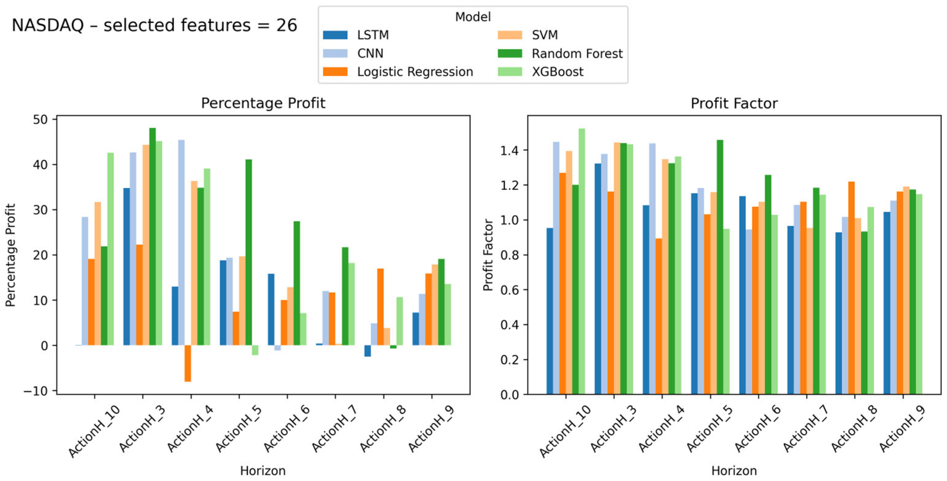
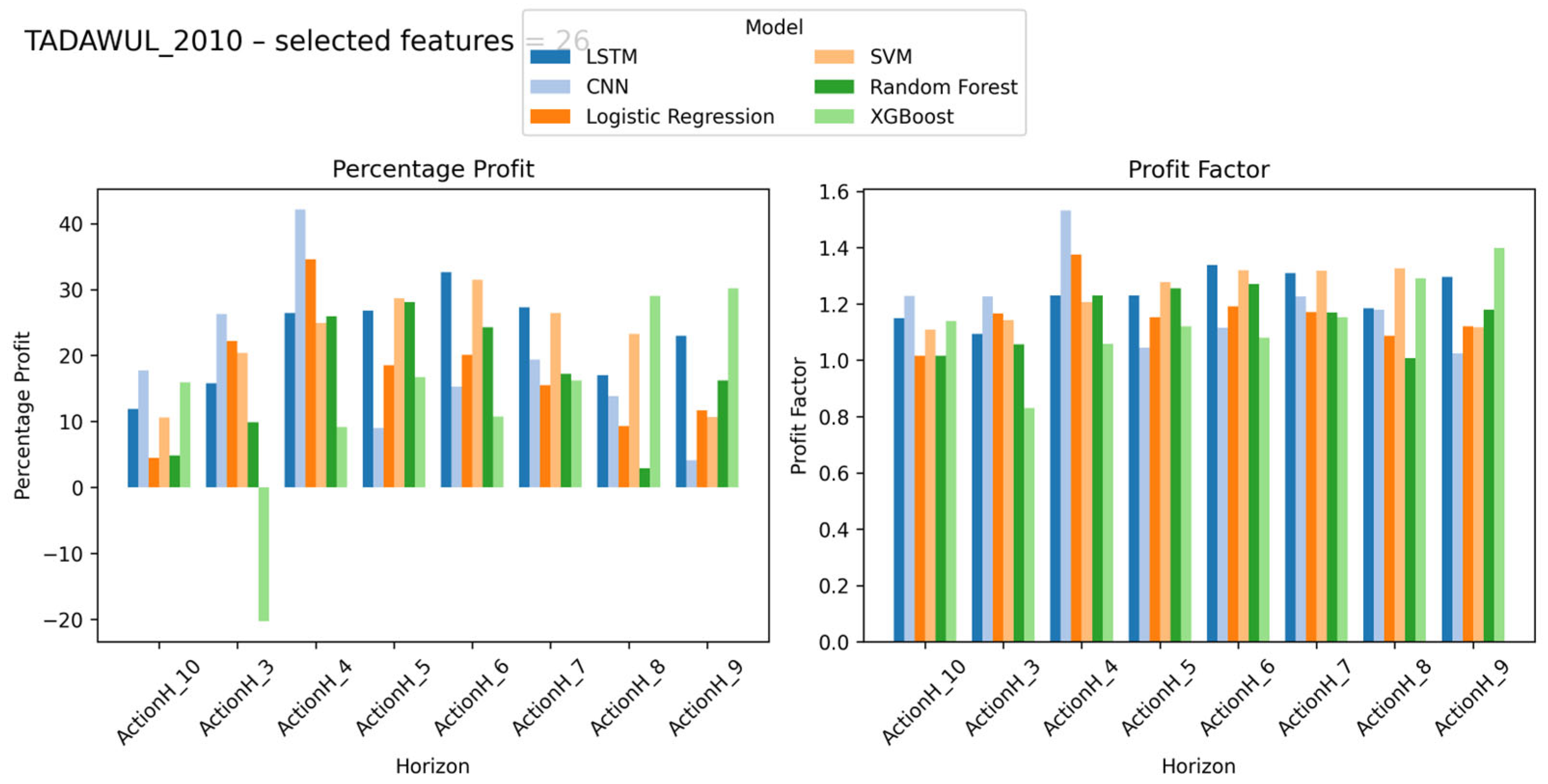
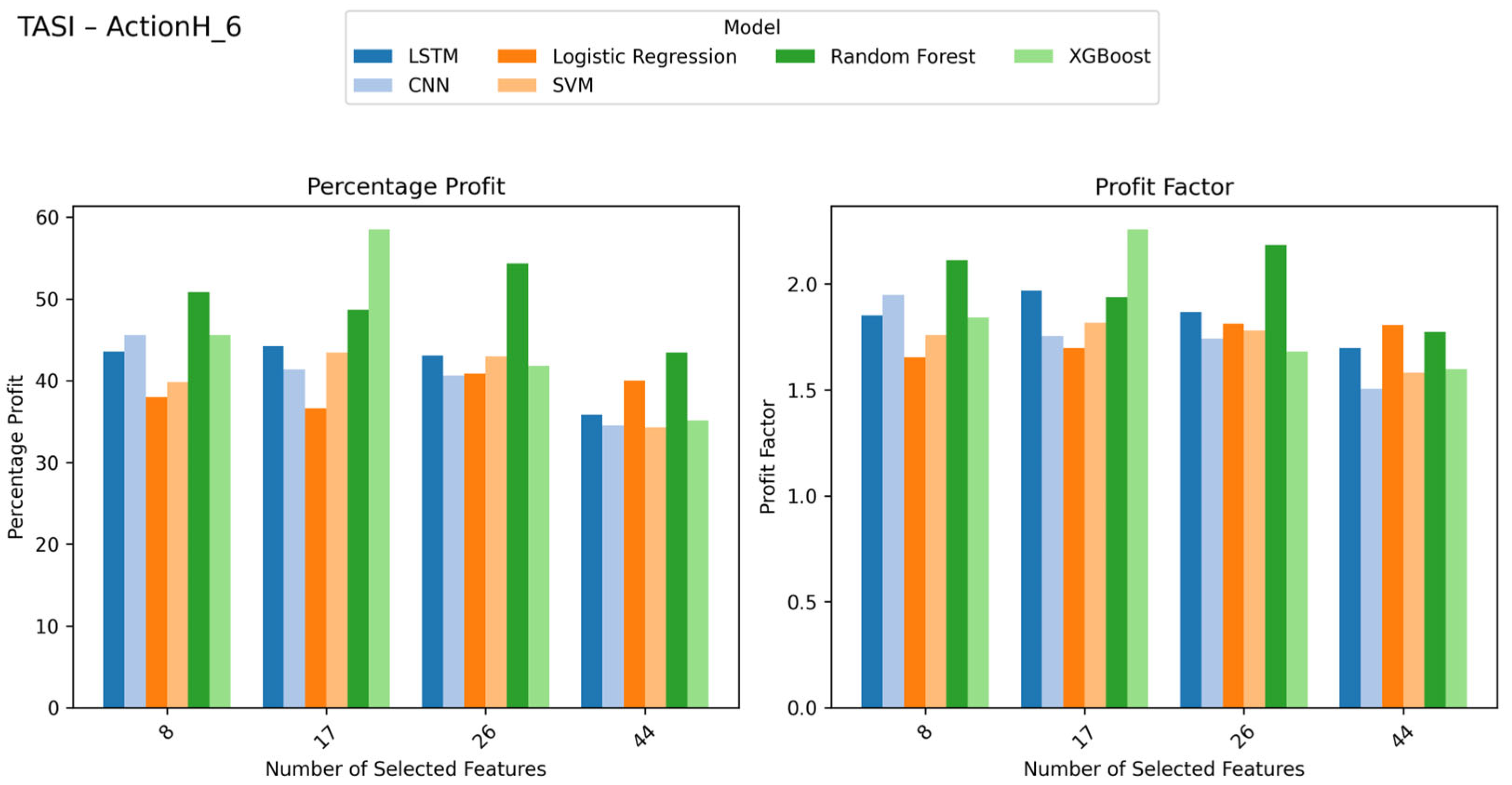
6.3. Top Resulted Graphs

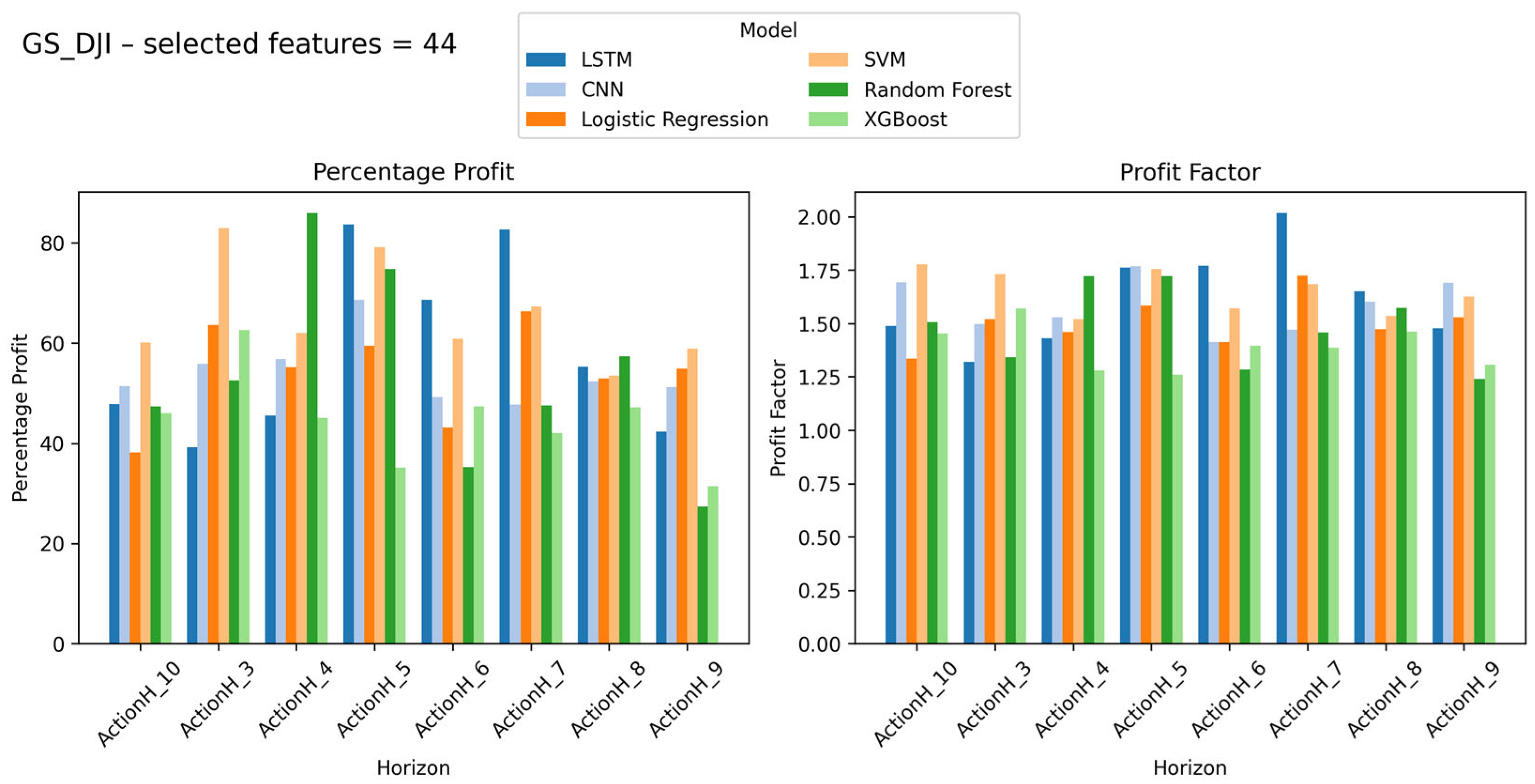
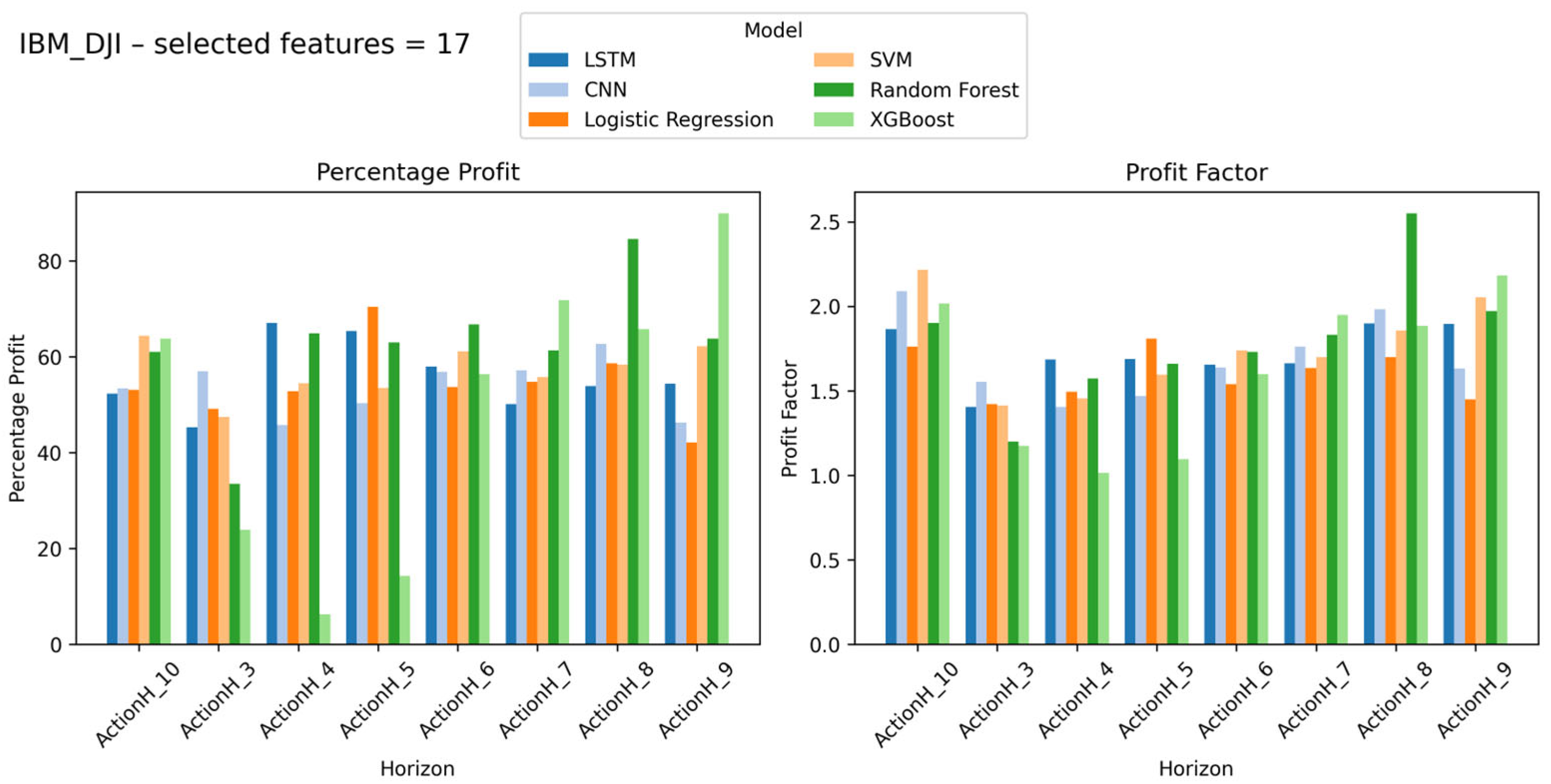
The results presented in Figure 2, Figure 3, Figure 4, Figure 5, Figure 6, Figure 7, Figure 8, Figure 9, Figure 10 and Figure 11 demonstrate a systematic evaluation of short-term trading strategies across multiple benchmarks and individual stocks. The framework highlights the importance of tailoring model configurations such as look-ahead windows, feature subsets, and algorithm selection to each asset’s unique market dynamics. For instance, while simpler models like logistic regression and XGBoost perform competitively in certain cases, deep learning approaches (LSTM, CNN) show superior profitability in high-volatility environments, as seen in tech-heavy indices and stocks. The optimal look-ahead horizon varies significantly, with liquid U.S. indices favoring shorter windows (e.g., 3 days) and less-liquid markets like TASI benefiting from longer horizons (6–10 days). Feature subset size also plays a critical role, with smaller subsets (e.g., 17 features) often sufficing for certain assets, while others require more granular inputs (e.g., 44 features).

Figure 2. TASI results with percentage profit and profit factor on Y-axis and look-ahead window on X-axis (number of selected features = 17).

Figure 3. DJI index results with percentage profit and profit factor on Y-axis and look-ahead window on X-axis (number of selected features = 44).

Figure 4. GS stock results with percentage profit and profit factor on Y-axis and look-ahead window on X-axis (number of selected features = 44).

Figure 5. IBM stock results with percentage profit and profit factor on Y-axis and look-ahead window on X-axis (number of selected features = 17).

Figure 6. NASDAQ index results with percentage profit and profit factor on Y-axis and look-ahead window on X-axis (number of selected features = 17).

Figure 7. NVDA index results with percentage profit and profit factor on Y-axis and look-ahead window on X-axis (number of selected features = 26).

Figure 8. TASI results with percentage profit and profit factor on Y-axis and Number of selected features on X-axis (Look-ahead window = 3).

Figure 9. SPX index results with percentage profit and profit factor on Y-axis and look-ahead window on X-axis (number of selected features = 44).

Figure 10. 2010 stock results with percentage profit and profit factor on Y-axis and look-ahead window on X-axis (number of selected features = 26).

Figure 11. TASI results with percentage profit and profit factor on Y-axis and number of selected features on X-axis (look-ahead window = 6).

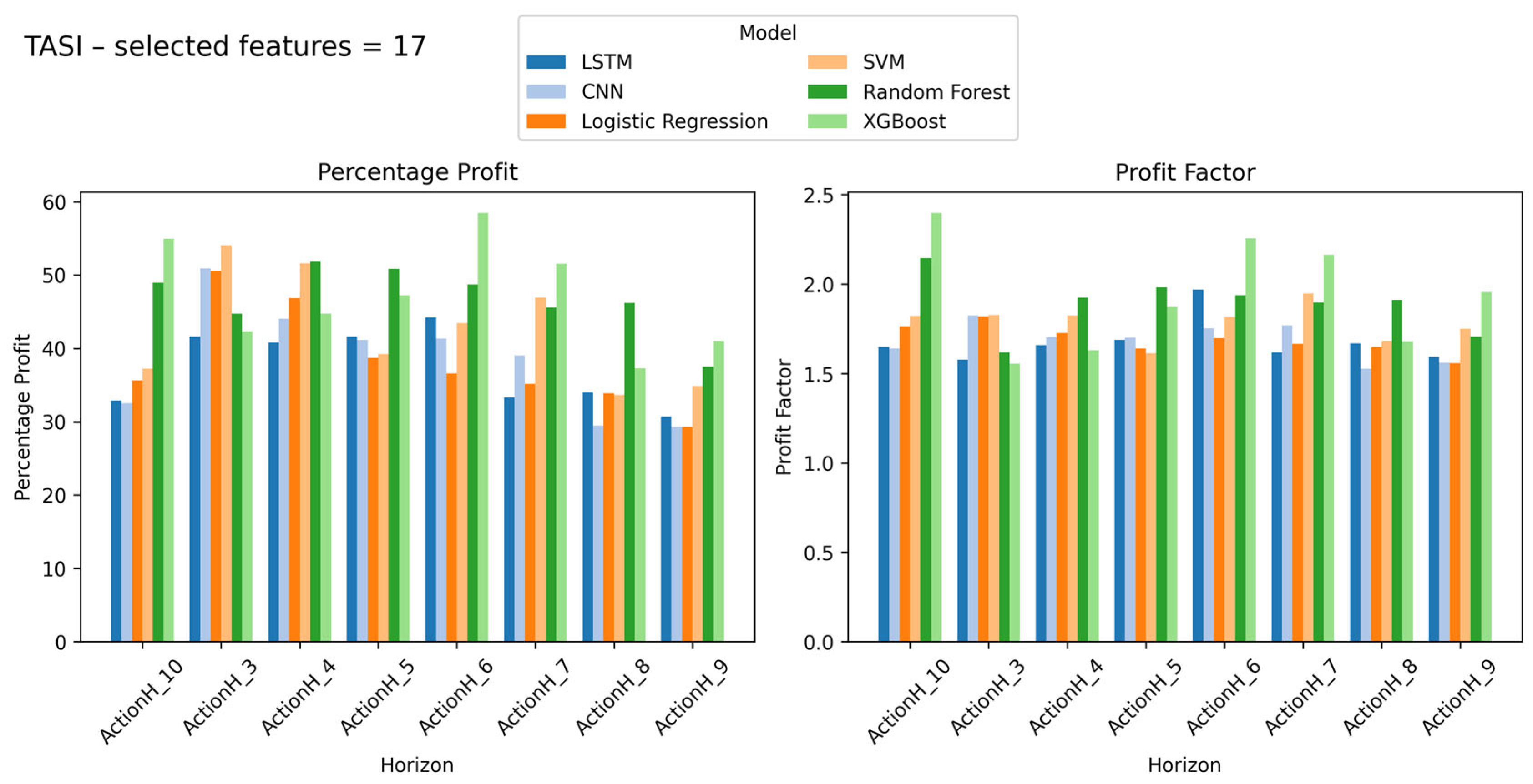
Figure 2 presents the comparative performance of six predictive models LSTM, CNN, Logistic Regression, SVM, Random Forest, and XGBoost applied to the TASI using 17 selected features. The two subplots display the Percentage Profit (left) and Profit Factor (right) across different prediction horizons labeled as Ahead-1, Ahead-3, Ahead-5, Ahead-7, and Ahead-9.

The ensemble models, Random Forest and XGBoost, show superior performance compared with the others across all horizons in terms of profitability and risk-adjusted returns. XGBoost produces the highest percentage profit, around 55–60% for shorter horizons, with Random Forest performing slightly lower. Neural network models, including LSTM and CNN, achieve moderate results with profits between 35–45%, while linear models such as Logistic Regression and SVM yield lower outcomes.

The Profit Factor results support the strength of the ensemble methods. Both XGBoost and Random Forest maintain values above 1.5, reflecting a strong ratio of gross profit to gross loss. Other models record profit factors around 1.2–1.5, indicating less stable profitability. It can also be seen that both predictive accuracy and profit tend to decline with longer forecasting horizons, showing that short-term market behavior is easier to predict than distant movements.

Across all tests, the Profit Factor and Percentage Profit metrics reveal that no single configuration dominates universally. Instead, the highest-performing strategies emerge from asset-specific optimization, reinforcing the framework’s core thesis: adaptive, label-aware modeling outperforms rigid, one-size-fits-all approaches. Figure 2, Figure 3, Figure 4, Figure 5, Figure 6, Figure 7, Figure 8, Figure 9, Figure 10 and Figure 11 collectively underscore the trade-offs between model complexity, feature relevance, and temporal alignment, providing actionable insights for deploying robust short-term trading systems.

6.4. Best Look-Ahead Window (Aggregate Analysis)

When aggregating across all instruments, the optimal look-ahead window was found to be 3 days, yielding the highest average Percentage Profit (around 30%). This was closely followed by 9-day (approximately 29%) and 10-day (approximately 28%) look-ahead windows. These results suggest that shorter-term forecasting horizons tend to provide a more reliable signal due to a lower noise-to-signal ratio in the immediate market response. However, this trend also indicates that shorter-term predictions are more adaptable and responsive to market fluctuations, which is crucial in fast-moving markets.

6.5. Model Popularity and Feature-Count Stability

XGBoost was the most popular model in terms of wins, securing 11 victories across the instruments studied (Table 7). Other models like Random Forest and CNN also performed well, particularly in specific contexts such as volatile or tech-focused stocks (e.g., NVDA and 2010). While LSTM had limited success, it was still able to perform well in specific cases where temporal dependencies were critical.

Table 7. Best Configurations for Each Index.

Index	Model	Look Ahead Window	% Profit
DJI	XGBoost	3	48%
NASDAQ	XGBoost	4	51%
SPX	XGBoost	5	46%
TASI	XGBoost	6	58%

The feature subset size, or dimensionality, that maximized percentage profit varied across different markets. For U.S. large-cap indices like SPX and DJI, a larger feature subset (44 variables) was optimal, capturing momentum and trend signals. In contrast, markets like TASI, characterized by lower liquidity, required fewer features (8–17 variables), as excessive dimensionality tends to overfit in such markets. This highlights the “curse of dimensionality” in low-liquidity environments, where fewer, more relevant features tend to provide better predictive power.

In terms of feature importance, momentum oscillators and volatility–volume hybrids emerged as the most influential indicators. The top-10 features, which include RSI, %K, ADX and MACD, captured most of the total importance across all instruments (Table 8). Notably, liquidity-driven variables were more important in markets such as TASI and NASDAQ, where order flow effects have a stronger impact. These findings suggest that in more liquid markets, momentum and trend-based features dominate, while in less liquid markets, factors related to volume and liquidity have a more substantial impact on performance.

Table 8. Most Important Chosen Features.

Rank	Factor Name
1	RSI
2	%K
3	ADX
4	MACD
5	Histogram
6	DI+
7	%R
8	ROC
9	CRSI
10	True Strength Index

6.6. Aggregated Feature–Importance Patterns

From the results, several best practices emerge for optimizing trading strategies using machine learning models. Firstly, for diversified baskets, starting with a look-ahead window of 3 tends to yield the best average performance. However, market-specific tuning is recommended, with shorter look-ahead windows for faster-reacting indices like DJI and longer windows for slower-reacting markets like TASI. XGBoost should be prioritized, while Random Forest is suitable when the feature count is low. CNN and LSTM models can be tested for more volatile or tech-focused stocks. Lastly, it is essential to avoid blindly transferring configurations from indices to their constituents, as only 25% of cases shared the same optimal look-ahead window.

7. Discussion and Analysis

In this section, we discuss the results thoroughly, with special attention to the responsiveness of the look-ahead windows, the relative performance of classical and deep learning methods, the portability of the results between different assets, contributions of individual features, and the influence of model architecture on feature importance.

7.1. Sensitivity of Look-Ahead Window

The sensitivity of performance to the length of the look-ahead window is a critical aspect of our analysis. Our research indicates that the look-ahead time may be increased to H ≥ 8. For example, longer horizons can provide more room for market corrections and reduce the impact of short-term fluctuations, making them particularly suitable for more stable indices such as the S&P 500 (SPX) and TASI, where preserving capital is often more important than maximizing raw returns.

Additionally, when the forecast horizon is shorter such as 3 days horizon, the models reported higher raw profit gains, not primarily for volatile assets such as NASDAQ and NVDA. As a result of their increased volatility day to day movements of these assets are more pronounced and short-term look-ahead windows enable the models capture these movements well. This creates a trade-off between return consistency (provided by longer look-ahead windows) and total return magnitude (driven by shorter horizons).

The findings show that the look-ahead window that is the most effective fluctuates greatly in different contexts. In volatile markets or markets with rapid price changes, a smaller horizon is more helpful in achieving high profitably. On the other hand, with stable priced indices or assets, use of a longer look ahead window could limit the production of false signals, thus increasing the consistency of results. A contingency of stability and return magnitude is revealed in this analysis as significant in selecting an optimal model setup for practitioners.

7.2. Classical Models vs. Deep Learning

One of the key findings in our study is the superior performance of XGBoost compared to deep learning models, particularly when evaluated on out-of-sample percentage profit across our 16-instrument universe. During our study, XGBoost, a classical tree-based technique consistently outperformed deep learning on out-of-sample trials, indicating that tree models are very good at recognizing subtle, but important correlations in financial structures. Such performance explicates that XGBoost, given its ability to process heterogeneous features and resolve overfitting, is a reliable tool for general financial predictions.

However, deep learning models, such as CNN and LSTM revealed their effectiveness in niche market scenario, particularly during times of increased volatility, such as with NVDA. In such cases, deep learning architectures far outperformed tree models, adding more than 250 basis points to returns over the top competing tree-based option. It illustrates how traditional models tend to be favored even though deep learning approaches shine in finding subtleties in patterns and interdependencies in highly turbulent financial numbers. Take NVDA as an example, its price being influenced by macroeconomic and technical dynamics, while by virtue of deep learning models’ expertise with sequence and hierarchical data NVDA has benefited.

The performance of deep learning models in high-volatility, tech-focused stocks implies that they are best used as tactical overlays rather than replacements for traditional models. When deployed strategically, deep learning architectures can offer enhanced returns in volatile markets, but in more stable environments, classical models like XGBoost remain preferable due to their simpler and more interpretable nature. This distinction is important for practitioners who seek to optimize their trading strategies based on market conditions.

7.3. Cross-Asset Transferability

The concept of cross-asset transferability is a central theme in this study. For seven out of the twelve constituents (58%), the index-optimal model also proved to be the stock-optimal model. This suggests that, in many cases, models trained on an index can be successfully transferred to its individual components, saving substantial computational resources in the process. Moreover, the reusability of models across related assets provides a significant advantage in terms of reducing the costs of grid searches and hyper parameter tuning.

However, while the model selection transferability is relatively high, the transferability of the look-ahead window was more limited. Only three constituents (25%) shared the same optimal look-ahead window as their respective index indicating that the optimal look-ahead window for a given index does not necessarily extend to its constituent stocks. This suggests that while model configurations may transfer effectively across assets, the look-ahead window must be re-tuned at the stock level for optimal performance.

The findings highlight the value of adopting a top-down approach to model deployment. Training on the index and then reusing the model on its constituents saves roughly 50% of the grid-search cost, while only a slight reduction in performance is observed, provided that look-ahead windows are fine-tuned locally. This strategy offers significant cost-saving opportunities without compromising the efficacy of the model.

7.4. Interpreting Feature Importance

The analysis of feature importance reveals that fast-acting oscillators and micro-structure proxies are consistently the most influential features across different models and assets. Notably, features such as the relative strength index (RSI) and ADX were dominant in many of the best-performing models. These features are highly sensitive to short-term price movements, indicating that market participants often react to immediate, technical signals, such as mean-reversion patterns and liquidity shocks, in a way that can be exploited by machine learning models.

The dominance of fast-acting features aligns with the behavioral finance view that markets exhibit short-term mean-reversion and are subject to liquidity-driven shocks. These findings suggest that practitioners should prioritize maintaining a clean, low-latency data feed for these signals, as they appear to be the most actionable in the context of financial forecasting. The marginal gain from incorporating longer-lag macroeconomic indicators appears limited, supporting the notion that focusing on shorter-term, high-frequency signals may provide better results.

7.5. Model and Feature Interactions

The interaction between features and models reveals important insights into the synergies between different model architectures and feature subsets. Classical models, such as XGBoost and Random Forest, benefit from reduced dimensionality, where a smaller number of features provides more effective decision boundaries. These models excel in capturing relationships between a limited set of strong signals, making them well-suited for structured data with a focus on trend-following or momentum.

In contrast, deep learning models, particularly CNNs and LSTMs, excel at extracting higher-order interactions from larger feature sets. Even when the number of features increases (up to 44 variables), deep models are capable of processing complex, non-linear relationships and temporal dependencies within the data. This ability to handle large feature subsets and model intricate patterns makes deep learning models particularly well-suited for high-dimensional problems, where the interactions between features are not immediately apparent.

These interactions between model types and feature sets suggest that a hybrid approach may be beneficial, where classical models are used for more stable, low-dimensional tasks, and deep learning models are employed for tasks that require higher-order pattern recognition and temporal sequence learning. This approach ensures that both the strengths of classical machine learning and deep learning models are leveraged to their fullest potential.

7.6. Market Microstructure and Performance Differences

The differing optimal models and labeling horizons between US markets and the Saudi TASI arise from fundamental market-microstructure distinctions.

• Liquidity and Settlement:

US equities exhibit high liquidity and rapid price discovery, supported by a shorter settlement cycle. TASI operates with lower liquidity and slower execution dynamics.

• Participant Mix and Volatility:

TASI’s higher retail participation produces slower, episodic volatility patterns, while US markets show more stable, institution-driven volatility structures.

• Impact on Forecasting Horizons:
  • TASI: Slower price adjustment favors longer prediction horizons.
  • US indices: High liquidity and fast information flow make shorter horizons more effective.

These structural differences explain why forecasting performance is market-dependent and why no single model–horizon combination generalizes across such heterogeneous environments.

8. Conclusions

This study presents a systematic methodology for building high-performing trading configurations across indices and individual stocks. By jointly exploring model choice, labeling horizon, and feature subsets, the framework identifies optimal settings for each asset while reducing dimensionality without sacrificing profitability. An important finding is the transferability of index-level configurations to constituent stocks, enabling a top-down approach where an index-trained model can guide stock-level training with minimal adjustments, mainly in look-ahead tuning.

Future work focuses on several extensions, i.e., online meta-learning and regime-aware reconfiguration for dynamic adjustment; realistic execution modeling (commission-slippage), latency, and market impact for closer alignment with live trading; analysis across market regimes (bull, bear, high-volatility) to identify horizon-dependent strengths and vulnerabilities; dynamic, volatility-responsive look-ahead windows using adaptive scaling or DTW-based selection to improve label quality; and realistic cost models to refine profitability. Once extended, the framework will include portfolio-level risk-adjusted metrics (Sharpe, Sortino, Maximum Drawdown) and statistical robustness analysis (t-tests, bootstrapping, horizon-wise confidence intervals) to support comprehensive significance testing and regime-aware robustness evaluation.