Abstract
We recall the normalized forms for the three Bessel-type functions; these functions are the Bessel function, Lommel function, and Struve function of the first kind. By using convolution, we define normalized forms. The essential purpose is to introduce necessary and sufficient bounds of these normalized functions so these functions are starlike and convex of order and type .
1. Introduction
We use the symbol to refer to the family of all functions that are analytic and univalent, with the normalization ; that is is expressed as
and the domain is the open unit disk . Also, let , consisting of functions with negative coefficients, which have the form
The Hadamard product (convolution) of will also be used; for this purpose it is defined by
Definition 1.
For and , let be the set of all functions ϕ (ϕ has the form (1)) satisfying the inequality
Also, take as the set of all functions ϕ (ϕ has the form (1)) that satisfy the inequality
and are the well-known subclasses of convex and starlike functions of order γ and type δ, respectively, introduced in [1].
- It is recognized that
Lemma 1.
Proof.
It is sufficient to show that
The last expression is bounded above by δ if the inequality (7) holds true, and hence the proof is completed. □
Lemma 2 ([1]).
Lemma 3.
Proof.
Since the proof is a direct consequence of Lemma 1 and the equivalence relation 6, we omit the details. □
Lemma 4 ([1]).
Recently, many researchers have considered specific categories of analytic functions, , that include particular functions. to determine the circumstances under which the members of exhibit certain geometric features, such as convexity, univalence, or starlikeness in . In this area, many studies about generalized hypergeometric functions are accessible in the literature [7,8]. In the field of geometric theory of functions of a complex variable, special functions like Bessel, Struve, and Lommel functions of the first kind have drawn a lot of attention. Motivated by certain previous advances, the geometric features of these special functions were recently studied. See [9,10,11,12,13], in which the univalence and starlikeness of Bessel functions of the first kind were taken into consideration. The radii of univalence, starlikeness, and convexity for the normalized forms of Bessel, Struve, and Lommel functions of the first kind have been determined in recent years; for example see [14,15,16,17,18,19,20,21,22,23,24].
Our study aims to provide some new conclusions about the convexity and starlikeness of the first-kind normalized Bessel, Struve, and Lommel functions. Now, we recall the first-kind Bessel function , the first-kind Struve function and first-kind Lommel function as follows, respectively.
and
Furthermore, we are aware that (see [25] (p. 217) and [26]) the homogeneous Bessel differential equation
has a solution in the form of the Bessel function
- And the Struve function is a particular solution of
This work is significant as it discusses geometric characteristics of several of the most popular special functions in mathematics (Lommel, Struve, and Bessel), such as convexity and starlikeness. We use convolution techniques for a class of univalent analytic functions to show these geometric features. After introducing the basic theorems and the required and sufficient criteria, we provide several interesting instances. We have provided figure calculations using the Maple tool.
We provide necessary and sufficient circumstances under which the first-kind normalized Lommel , first-kind normalized Struve , and first-kind normalized Bessel functions fall into certain families of analytic functions.
2. Results Regarding Lommel Functions
For the sake of simplicity or brevity, we shall use that and throughout this article until otherwise noted. If
and applying convolution, then we introduce , which is defined by
which is a modified normalized Lommel-type function. Actually, we have defined this form by convolution so that the function , for which the first investigation is introduced.
Theorem 1.
Proof.
Here
By using Lemma 1, it is sufficient to give that
We have
Then
is bounded above by if inequality (23) is satisfied. This completes the proof. □
The following result introduce a necessary and sufficient condition. For this purpose let
Also, by applying convolution, the function is given by
Indeed, we have defined this form by convolution so that the function , where T is the subclass of functions with negative real coefficients defined in (2).
Theorem 2.
If , then inequality (23) is the necessary and sufficient condition to have .
Proof.
Simply, we can verify that
using Lemma 1 in conjunction with the methods described in Theorem 1. We have already provided the proof of Theorem 2. □
Now, we introduce the convex results.
Theorem 3.
Proof.
Similarly, we give the necessary and sufficient theorem for convexity.
Theorem 4.
If , then the inequality given by (28) is the necessary and sufficient condition for .
Corollary 1.
The function if and only if
Corollary 2.
The function if and only if
3. Results Regarding Struve Functions
Putting in Theorems 1–4, we obtain the matching Struve function results, which are as follows.
Theorem 5.
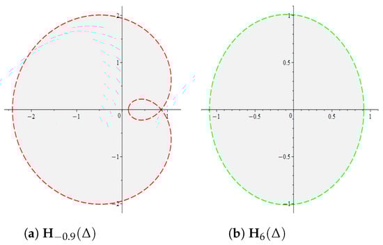
Taking and in Theorem 5 leads us to the following illustrative example.
Example 1.
If , then the function ; i.e., is a starlike function. We list the following cases for different values of as follows:
Theorem 6.
If , then the inequality (32) is necessary and sufficient to have such that
Theorem 7.
If , then the condition
suffices to ensure that
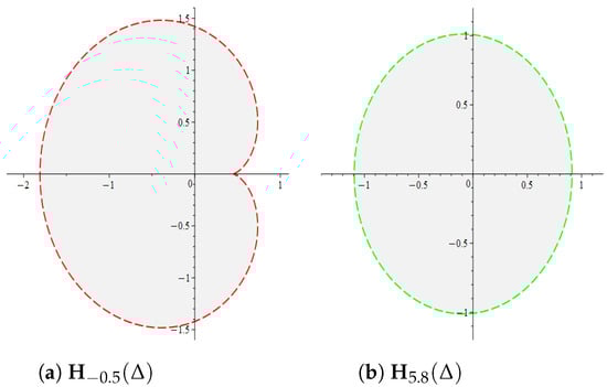
Taking and in Theorem 7 leads us to following illustrative example.
Example 2.
If , then the function ; i.e., is a convex function. We list the following cases for different values of as follows:
Theorem 8.
If , then the inequality (35) is necessary and sufficient to have .
Corollary 3.
The function if and only if
Corollary 4.
The function if and only if
4. Results Regarding Bessel Functions
Apply the restriction in Theorems 1–4; then we derive the appropriate Bessel function results, which are shown below.
Theorem 9.
Taking and in Theorem 9 leads us to following illustrative example.
Example 3.
If , then the function ; i.e., is a starlike function. We list the following cases for different values of as follows:
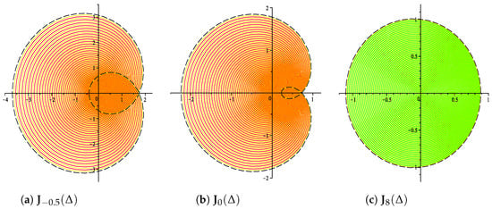 Figure 3. for different values of p.
Theorem 10.
If , then inequality (38) is necessary and sufficient to have , where
Theorem 11.
If , then the inequality
suffices to ensure that
Taking and in Theorem 11 leads us to following illustrative example.
Example 4.
If , then the function ; i.e., is a convex function. We list the following cases for different values of as follows:
Theorem 12.
If , then relation (41) is necessary and sufficient to have .
Corollary 5.
The function if and only if
Corollary 6.
The function if and only if
Taking in Corollaries 5 and 6 leads us to following illustrative example.
Example 5.
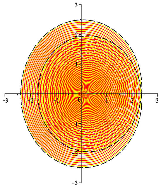
For the function we have the following equivalences:
and
Choosing , we notice that
Similarly,
because the function and ; see Figure 4 below.
Figure 4.
The range .
5. Conclusions
The familiar Bessel function, Lommel function, and Struve function of the first kind are the three Bessel-type functions for which we utilized the normalized forms. These normalized forms were defined using the convolution operation. The main goal was to provide sufficient and necessary constraints for these normalized functions, making them starlike and convex of type and order . For future work, we recommend applying the convolution technique that has been used in this article to investigate the starlikeness and convexity of some other special functions of a complex variable, such as the Mittag–Leffler function [27], Hurwitz–Lerch Zeta function [28], and hypergeometric functions [29], and also other geometric properties, such as close to convexity. Additionally, the multivalent case of functions can be studied.
Author Contributions
Conceptualization, R.A., S.A., R.M.E.-A. and A.H.E.-Q.; methodology, R.M.E.-A., S.A., R.A. and A.H.E.-Q.; software, A.H.E.-Q. and S.A.; validation, R.M.E.-A., S.A., A.H.E.-Q. and R.A.; formal analysis, S.A., R.A. and A.H.E.-Q.; investigation, R.A., R.M.E.-A., S.A. and A.H.E.-Q.; resources, A.H.E.-Q., S.A. and R.M.E.-A.; data curation, R.A.; writing—original draft preparation, R.M.E.-A. and A.H.E.-Q.; writing—review and editing, R.M.E.-A., S.A. and R.A.; visualization, R.A. and R.M.E.-A.; supervision, R.M.E.-A. and A.H.E.-Q.; project administration, S.A. and R.A.; funding acquisition, S.A. All authors have read and agreed to the published version of the manuscript.
Funding
This work was supported and funded by the Deanship of Scientific Research at Imam Mohammad Ibn Saud Islamic University (IMSIU) (grant number IMSIU-DDRSP2503).
Data Availability Statement
No new data were created or analyzed in this study.
Conflicts of Interest
The authors declare that there are no conflicts of interest.
References
- Gupta, V.P.; Jain, P.K. Certain classes of univalent functions with negative coefficients. Bull. Austral. Math. Soc. 1976, 14, 409–416. [Google Scholar] [CrossRef]
- Robertson, M.S. On the theory of univalent functions. Ann. Math. 1936, 37, 374–408. [Google Scholar] [CrossRef]
- Schild, A. On starlike function of order α. Am. J. Math. 1965, 87, 65–70. [Google Scholar] [CrossRef]
- MacGregor, T.H. The radius of convexity for starlike function of order α. Proc. Am. Math. Sec. 1963, 14, 71–76. [Google Scholar]
- Goodman, A.W. Univalent Functions; Mariner: Tampa, FL, USA, 1983; Volume 1–2. [Google Scholar]
- Silverman, H. Univalent functions with negative coefficients. Proc. Am. Math. Soc. 1975, 51, 109–116. [Google Scholar] [CrossRef]
- Mocanu, S.S.; Miller, P.T. Univalence of Gaussian and confluent hypergeometric functions. Proc. Am. Math. Soc. 1990, 110, 333–342. [Google Scholar] [CrossRef]
- Singh, S.; Ruscheweyh, V. On the order of starlikeness of hypergeometric functions. J. Math. Anal. Appl. 1986, 113, 1–11. [Google Scholar] [CrossRef]
- Brown, R.K. Univalence of Bessel functions. Proc. Am. Math. Soc. 1960, 11, 278–283. [Google Scholar] [CrossRef]
- Brown, R.K. Univalent solutions of W″ + pW = 0. Canad. J. Math. 1962, 14, 69–78. [Google Scholar] [CrossRef]
- Brown, R.K. Univalence of normalized solutions of W″(z) + p(z)W(z) = 0. Int. J. Math. Math. Sci. 1982, 5, 459–483. [Google Scholar] [CrossRef]
- Kreyszig, E.; Todd, J. The radius of univalence of Bessel functions. Ill. J. Math. 1960, 4, 143–149. [Google Scholar] [CrossRef]
- Wilf, H.S. The radius of univalence of certain entire functions. Ill. J. Math. 1962, 6, 242–244. [Google Scholar] [CrossRef]
- Aktaş, I.; Baricz, Á.; Yağmur, N. Bounds for the radii of univalence of some special functions. Math. Ineq. Appl. 2017, 20, 825–843. [Google Scholar]
- Baricz, Á. Geometric properties of generalized Bessel functions of complex order. Mathematica 2006, 48, 13–18. [Google Scholar]
- Baricz, Á. Geometric properties of generalized Bessel functions. Publ. Math. Debr. 2008, 73, 155–178. [Google Scholar] [CrossRef]
- Baricz, Á.; Kupán, P.A.; Szász, R. The radius of starlikeness of normalized Bessel functions of the first kind. Proc. Am. Math. Soc. 2014, 142, 2019–2025. [Google Scholar] [CrossRef]
- Baricz, Á.; Orhan, H.; Szász, R. The radius of α-convexity of normalized Bessel functions of the first kind. Comput. Methods Funct. Theory 2016, 16, 93–103. [Google Scholar] [CrossRef]
- Baricz, Á.; Ponnusamy, S. Starlikeness and convexity of generalized Bessel functions. Integral Transform. Spec. Funct. 2010, 21, 641–653. [Google Scholar] [CrossRef]
- Baricz, Á.; Szász, R. The radius of convexity of normalized Bessel functions of the first kind. Anal. Appl. 2014, 12, 485–509. [Google Scholar] [CrossRef]
- Baricz, Á.; Szász, R. Close-to-convexity of some special functions. Bull. Malay. Math. Sci. Soc. 2016, 39, 427–437. [Google Scholar] [CrossRef]
- Baricz, Á.; Yağmur, N. Geometric properties of some Lommel and Struve functions. Ramanujan J. 2017, 42, 325–346. [Google Scholar] [CrossRef]
- Szász, R. On starlikeness of Bessel functions of the first kind. In Proceedings of the 8th Joint Conference on Mathematics and Computer Science, Komárno, Slovakia, 14–17 July 2010; 9p. [Google Scholar]
- Szász, R.; Kupán, P.A. About the univalence of the Bessel functions. Stud. Univ. Babeş-Bolyai Math. 2009, 54, 127–132. [Google Scholar]
- Olver, F.W.J.; Lozier, D.W.; Boisvert, R.F.; Clark, C.W. (Eds.) NIST Handbook of Mathematical Functions; Cambridge University Press: Cambridge, UK, 2010. [Google Scholar]
- Watson, G.N. A Treatise of the Theory of Bessel Functions; Cambridge University Press: Cambridge, UK, 1995. [Google Scholar]
- Ali, E.E.; El-Ashwah, R.M.; Kota, W.Y.; Albalahi, A.M. Geometric attributes of analytic functions generated by Mittag-Leffler function. Mathematics 2025, 13, 3284. [Google Scholar] [CrossRef]
- Ali, E.E.; El-Ashwah, R.M.; Albalahi, A.M.; Sidaoui, R. Fuzzy treatment for meromorphic classes of admissible functions connected to Hurwitz–Lerch zeta function. Axioms 2025, 14, 523. [Google Scholar] [CrossRef]
- Ali, E.E.; El-Ashwah, R.M.; Aouf, M.K. On sandwich theorems for some subclasses defined by generalized hypergeometric functions. Stud. Univ. Babeş-Bolyai Math. 2017, 62, 89–99. [Google Scholar] [CrossRef]
Disclaimer/Publisher’s Note: The statements, opinions and data contained in all publications are solely those of the individual author(s) and contributor(s) and not of MDPI and/or the editor(s). MDPI and/or the editor(s) disclaim responsibility for any injury to people or property resulting from any ideas, methods, instructions or products referred to in the content. |
© 2025 by the authors. Licensee MDPI, Basel, Switzerland. This article is an open access article distributed under the terms and conditions of the Creative Commons Attribution (CC BY) license (https://creativecommons.org/licenses/by/4.0/).