Abstract
Accurate cooling load forecasting in high-efficiency chiller plants with ice storage systems is essential for intelligent control, energy conservation, and maintaining indoor comfort. However, conventional forecasting methods often struggle to model the complex nonlinear dependencies among influencing variables, limiting their predictive performance. To address this, this paper introduces Time-LLM, a novel time series forecasting framework that leverages a frozen large language model (LLM) to improve the accuracy and generalization of cooling load forecasting. Time-LLM extracts features from historical data, reformulates them as natural language prompts, and uses the LLM for temporal sequence modeling; a linear projection layer then maps the LLM output to final predictions. To enable lightweight deployment and improve temporal feature prompting, we propose ETime-LLM, an enhanced variant of Time-LLM. ETime-LLM significantly reduces deployment costs and mitigates the original model’s response lag during trend transitions by focusing on possible turning points. Extensive experiments demonstrate that ETime-LLM consistently outperforms or matches state-of-the-art baselines across short-term, long-term, and few-shot forecasting tasks. Specifically, in the commonly used 24 h forecasting horizon, compared with the original model, ETime-LLM achieves an approximately 17.3% reduction in MAE and a 19.3% reduction in RMSE. It achieves high-quality predictions without relying on costly external data, offering a robust and scalable solution for green and energy-efficient HVAC system management.
MSC:
37M10
1. Introduction
1.1. Research Background
The Chinese government has committed to establishing an ecologically friendly energy model by 2035 and achieving carbon neutrality by 2060 [1]. The Green and High-Efficiency Cooling Action Plan aims to improve cooling efficiency in large public buildings by 30% and refrigeration efficiency by over 25% by 2030, with an estimated electricity saving of 400 billion kWh annually [2]. As approximately 50% of a building’s energy consumption comes from environmental and temperature control systems [3,4], improving the energy efficiency of these systems is crucial for reducing carbon emissions.
High-efficiency chiller plants based on ice thermal energy storage play a vital role in ensuring the stable operation of large-scale HVAC systems. These plants integrate centralized control systems, dynamic optimization algorithms, and artificial intelligence techniques to minimize equipment power consumption while meeting cooling load, thereby significantly improving overall energy performance. However, accurate cooling load forecasting is critical for optimizing ice thermal energy storage systems, as inaccurate predictions can lead to excess ice production, energy waste, or insufficient storage, forcing the system to operate chillers during peak electricity pricing periods [5].
Cooling loads in buildings are typically periodic and multi-peak, influenced by external meteorological factors [6], making accurate prediction challenging. Thus, accurate cooling load forecasting is essential for energy conservation and emissions reduction. It helps minimize energy costs, reduces the operation time of equipment under suboptimal conditions, extends system lifespan, and supports the transition of HVAC systems to more intelligent and environmentally friendly operations, aligning with the long-term goal of carbon neutrality by 2060.
To achieve accurate cooling load forecasting, two primary approaches are commonly used: mechanism-based and data-driven modeling [7,8]. Mechanism-based models use thermodynamic principles and physical characteristics to create heat balance models, offering high interpretability but requiring detailed building information and being computationally expensive. These models are less suitable for complex buildings. In contrast, data-driven models use historical HVAC data to learn nonlinear relationships between inputs and cooling loads. These models are more flexible, require fewer assumptions, and are well-suited for real-time forecasting in existing buildings without detailed structural data. Due to their adaptability and accuracy, data-driven methods are increasingly popular for cooling load forecasting.
1.2. Related Works
Recent advances in deep learning have significantly improved data-driven time series forecasting. Compared with traditional machine learning, deep learning models can automatically learn complex nonlinear temporal patterns through multilayer neural architectures, reducing reliance on manual feature engineering and enabling more accurate multi-step forecasting [9,10]. Consequently, deep learning has become a dominant approach in cooling load forecasting.
Various models have been developed. Huang et al. optimized a Wavelet Neural Network(WNN) using Ant Colony Optimization, achieving substantial accuracy gains [11]. Dong et al. proposed an improved LSTM model for hourly cooling load forecasting, outperforming several LSTM variants [12]. Qu et al. applied PatchTST for multi-step, multi-task load forecasting, achieving high accuracy [13]. Studies further show that LSTM and Transformer models are well-suited for short- and long-term forecasting, respectively [14,15]. The Temporal Fusion Transformer (TFT) [16], integrating GRNs, multi-head attention, and VSNs, has demonstrated strong robustness in energy-related forecasting tasks [17]. Its ability to effectively capture long- and short-term dependencies, model complex interactions across multiple time scales. Additionally, TFT’s interpretability allows for a clearer understanding of how it handles multi-dimensional data.
Overall, while deep learning has been widely applied in power load forecasting and energy system analysis [18], its use in commercial building cooling load forecasting remains limited. Cooling load is influenced by comfort constraints, equipment operation, occupant behavior, and weather conditions, making direct model transfer difficult. Thus, tailored feature engineering and model adaptation are essential for accurate cooling load forecasting in complex and dynamic HVAC environments.
With the successful application of large language models (LLM) in natural language processing, researchers have begun to explore their potential for non-linguistic tasks, such as financial analysis [19,20] and time series forecasting [21]. Unlike traditional models, which require task-specific architectures, LLMs can be guided by prompt-based adjustments and have an inherent ability to capture long-range dependencies, making them suitable for time series modeling. At present, LLM-based time series forecasting methods have been applied to areas such as smart grids and electric submersible pump maintenance [22,23]. As shown in Table 1. But their application to cooling load forecasting remains underexplored and warrants further investigation.

Table 1.
Current application progress in time series forecasting.
In this study, we propose an enhanced temporal feature forecasting framework based on Time-LLM [26], named ETime-LLM, designed for efficient and accurate building cooling load forecasting on consumer-grade edge devices. This localized forecasting capability enables real-time decision-making for ice storage systems. Historical operational data are first restructured using prompt prefixing and patch reprogramming, converting continuous time series data into semantically meaningful textual prompts. To leverage the inherent capacity of LLM architectures to model long-range dependencies learned from large-scale language corpora, ETime-LLM reformulates cooling-load time series as a pseudo-linguistic sequence. The BERT-base model is employed as the backbone LLM within our framework [27], balancing deployment cost and prediction accuracy. Finally, a flattening operation followed by a linear projection produces the final time series predictions.
The main contributions of this paper are summarized as follows:
- This work is the first to investigate the application of LLM-assisted time series forecasting for cooling load forecasting in commercial buildings. By deploying a frozen LLM at the edge or terminal level and combining it with historical building data, the model enables accurate forecasting of future cooling loads, providing essential support for proactive HVAC parameter tuning. The results demonstrate the promising potential of LLMs in this domain.
- A lightweight BERT-base model is deployed as the backbone LLM strikes an effective balance between model adaptability and computational efficiency. It achieves competitive forecasting accuracy while significantly reducing training time, hardware overhead, and reliance on costly external data sources.
- The improved temporal feature attention mechanism is embedded prompt as prefix. Experimental results demonstrate that, compared to the original version, this mechanism effectively alleviates the prediction response lag during trend transitions in long-term time series forecasting.
2. Enhance-Time-LLM Forecasting Framework
Time-LLM is an innovative framework for time series forecasting that integrates the powerful feature extraction capabilities of LLMs with temporal analysis techniques. This framework is specifically designed to capture complex temporal patterns and long-term dependencies inherent in time series data. By leveraging the self-attention mechanism of LLMs, Time-LLM can model both short- and long-range temporal relationships, which is critical for multi-step forecasting tasks. The “innate ability” of LLMs to capture long-term dependencies comes from their pre-trained self-attention architecture, which enables the model to retain and focus on relevant information over extended time horizons. Additionally, by employing a frozen LLM, Time-LLM significantly reduces computational overhead, while maintaining or even enhancing the model’s ability to generalize from past data. The framework of the algorithm is shown in Figure 1. It first applies Fast Fourier Transform (FFT) to extract periodic features from historical data. Then, a prompt generator constructs optimized input representations, which are further transformed through patch-based reprogramming and alignment to create LLM-compatible input sequences. The assembled sequence of patches is then fed into the LLM, where temporal dependencies are modeled through contextual representation learning. The output of the LLM is subsequently passed through a linear projection layer to map the high-dimensional representations back into the target prediction space, resulting in the final forecasted time series. The overall framework consists of three main components: input transformation and preprocessing, frozen LLM backbone, and a linear projection module for final output generation.
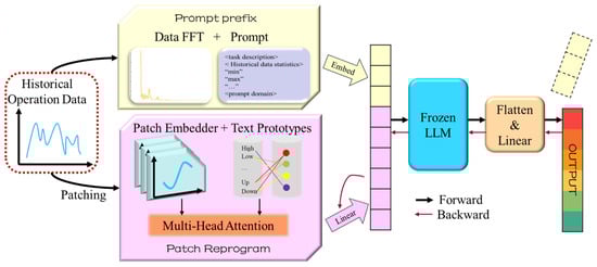
Figure 1.
The framework of Time-LLM. The yellow part is the prompt prefix module, and the pink part is the patch reprogramming module.
2.1. Input Transformation and Preprocessing
Typical time series inputs are typically represented as fixed-dimensional matrices, which are difficult for language models to interpret directly. The main idea of Time-LLM is to employ Temporal Reprogramming, a technique that transforms numerical time series data into prompt sequences compatible with language-based structures. To convert historical data files into patch-based inputs that can be processed by LLMs, Time-LLM first extracts periodic patterns and trend features from the raw data. Time series data are inherently composed of continuous numerical signals, whereas LLMs are primarily designed to handle discrete language tokens—creating a fundamental representational gap between the two modalities. Consider a set of time series data denoted by , where T denotes the total number of time steps, can be transformed into the frequency domain using the FFT. This transformation captures the underlying periodic structure of the sequence and is mathematically defined as:
In this expression, represents the complex-valued spectral coefficient at the normalized frequency f, is the time-domain observation at timestep t, and the exponential term serves as the basis function that projects the time series onto the frequency domain, the symbol j denotes the imaginary unit, which satisfies the identity . While statistical feature extraction and FFT enable the LLM to capture overall trends and short-term patterns, they lack explicit positional information, making it difficult for the model to respond promptly to trend transitions in cooling load sequences. To address this limitation, in addition to the periodic lag parameters calculated through the autocorrelation function, ETime-LLM considers the trend change position parameters as prompt input. Specifically, the autocorrelation coefficient are computed as (2):
where is the value of the time series at time t, is the mean of the sequence, and T denotes the total length of the sequence. Higher values of indicate stronger similarity between the current series and its lag-k version. Given a predefined lag L, the first-order difference is calculated as a transition from sustained positive to negative differences (or vice versa) indicates a potential trend reversal. By sliding this computation across the time series and monitoring the sign and magnitude changes of , the model can effectively detect inflection points. These points are then used to enhance temporal feature prompting, enabling improved responsiveness during structural changes in load patterns.
To enhance the model’s generalization capability on non-stationary data, the 0–1 normalization is introduced. It normalizes each sample individually, significantly mitigating the impact of inconsistent feature scales and helping to prevent issues such as gradient vanishing or explosion [28].
Based on Equation (1), continuous temporal data can be effectively transformed into discrete variables, revealing the periodic characteristics embedded in the sequence. The input time series is segmented into patches, analogous to the tokenization process in natural language processing (NLP). Specifically, Time-LLM divides an original time series of length L into multiple overlapping patches of fixed length , using a sliding window with stride S. A historical sequence is thus segmented into a set of patches , where denotes the total number of patches. The i-th patch is formally defined as:
here, represents the observation at time step t, is the patch length, S is the stride of the sliding window, and m is the total number of patches obtained from the segmentation process. This overlapping patching strategy enables the model to capture both local temporal features and global sequential dependencies effectively.
To adapt the input structure of LLMs and achieve modality alignment, Time-LLM introduces patch reprogramming mechanism. This module learns an attention-based reprogramming process using a set of compact textual prototypes derived from long-range time series data. Without modifying the architecture of the LLM, it enables the mapping of time series patches into the word embedding space of the language model. A subset of the language model’s word embeddings is selected, and a multi-head cross-attention mechanism is employed to align the modalities. Each time series patch is projected into a high-dimensional feature space using a linear embedding layer , producing patch embeddings. These embeddings are then reassembled into the pretrained semantic space of the language model. This step effectively bridges the gap between continuous time series data and discrete language symbols, enabling the LLM’s reasoning capabilities to directly utilize temporal information.
Building upon the concept of prompt learning, Time-LLM incorporates the Prompt-as-Prefix (PaP) strategy, where task descriptions, statistical features (e.g., maximum, minimum, trend, lag and inflection point), and domain knowledge are formatted as natural language and prepended to the input sequence. This prefix guides the language model in performing semantic reasoning specific to the time series forecasting task. Within the hierarchical prompt structure, the task description steers the LLM to adapt patch embeddings toward the given task. The statistical features are integrated into the prompt text, blending foundational dataset knowledge with task-specific details to enhance pattern recognition and inference capabilities. The resulting input structure is as follows:
The final prompt construction in this work follows a structured format as Figure 2. It concatenates the task description, statistical attributes, temporal features, and reprogrammed patch embeddings to form the full input prompt for the language model.
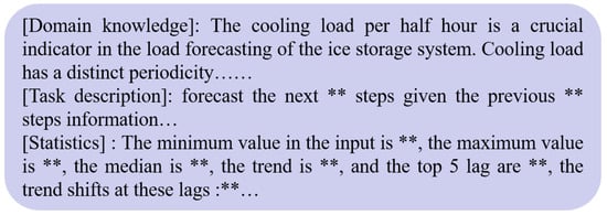
Figure 2.
An instance of the prompt converted from patch, ** is the parameter set as required.
2.2. Lightweight Backbone Model Inference and Prediction
Different from conventional Transformer-based models that rely on parameter updates during training, Time-LLM utilizes a frozen LLM, such as Qwen [29], LLaMA [30], or GPT2 [31] as a temporal pattern generator. Its parameters remain unchanged throughout the process, and prediction is guided solely by prefix-based prompts. The prompts assembled in Section 2.1 are fed into the backbone LLM, which, having been pretrained on vast corpora encompassing natural language, code, and structured data, possesses strong temporal generalization capabilities. As long as the prompts are sufficiently informative, the model can perform forecasting on unseen data domains. This strategy effectively mitigates the substantial computational overhead and overfitting risks typically associated with fine-tuning large-scale models.
In ETime-LLM, BERT is adopted as the foundational language representation model. BERT is a bidirectional pre-trained language model based on the Transformer architecture, designed to enhance contextual understanding in natural language processing tasks [27]. It is pre-trained on large-scale corpora, using Masked Language Modeling and Next Sentence Prediction to capture rich linguistic patterns. Unlike traditional unidirectional language models, BERT processes text bidirectionally, enabling deep semantic modeling at both the sentence and word levels. It has been widely applied to various NLP tasks such as question answering, named entity recognition, and text classification. BERT offers variants with different parameter scales, including BERT-Base (110 million parameters) and BERT-Large (340 million parameters). It has achieved state-of-the-art performance on several NLP benchmarks, including GLUE, SQuAD, and SWAG, significantly surpassing prior models.Compared to larger-scale models such as LLaMA and Qwen, BERT offers a more lightweight architecture with lower computational requirements, making it more suitable for resource-constrained environments. Thanks to its strong transferability, BERT can still deliver competitive performance on downstream tasks even with limited annotated data. In this work, BERT-Base is employed as the backbone encoder of the Time-LLM framework, integrated with the time reprogramming module and prompt-driven forecasting process, thereby enhancing the robustness and generalization capability of time series modeling while maintaining high efficiency. Table 2 summarizes the model sizes and training speeds of several LLMs, with their corresponding hardware configurations provided in Section 3.3. All models are evaluated under fp16 precision, and the reported model sizes include auxiliary components such as the tokenizer. It can be observed that BERT-base exhibits clear advantages in both training efficiency and deployment requirements.
Table 2.
Key parameters and runtime comparison of representative LLMs.
2.3. Flattened Output Projection
After obtaining the high-dimensional output tensor O from the frozen LLM, the prefix portion is first removed. A flattening linear projection layer then transforms O into the original temporal structure. This is achieved by flattening the tensor and applying a learnable weight matrix and bias vector, which project the representation into the target forecasting dimension. The final predicted sequence can be expressed as:
where denotes the portion of O corresponding to the time-series patches (excluding the prompt tokens), is the projection matrix, and is the bias term.
In summary, Time-LLM converts continuous time series data into input tokens compatible with large language models through prompt-based prefixing and patch reprogramming. By leveraging the language modeling and contextual attention capabilities of the LLM, it generates high-dimensional predictive representations. A subsequent flattening and linear projection layer then maps these representations into meaningful temporal forecasts. ETime-LLM introduces two key enhancements: an improved temporal feature encoding mechanism and a lightweight BERT-based embedding backbone. These modifications significantly reduce deployment and runtime costs while maintaining prediction accuracy, thereby achieving a balance between forecasting performance and computational efficiency.
3. Experimental Results
3.1. Engineering Scene Description
The historical cooling load data used in this study were collected from a comprehensive commercial center located in Fujian Province, China, which integrates multiple functions including shopping, dining, entertainment, and accommodation. The building is equipped with a high-efficiency air conditioning plant based on an ice thermal storage system to maintain indoor thermal comfort. The system comprises one dual-mode chiller, two base-load chillers, several cooling towers and water pumps, along with other essential auxiliary components, with a total rated power of 2173 kW. It operates under a dual-pipe closed-loop PID control scheme, as illustrated in Table 3.
Table 3.
Equipment and Operating Parameters List.
3.2. Data Processing and Analysis
During operation, sensors may experience faults, noise interference, or calibration issues, leading to anomalies and missing values in the dataset. To mitigate these unfavorable factors, this study employs the interquartile range (IQR) method to correct outliers, followed by cubic spline interpolation to impute missing values. These procedures are applied to the original dataset provided by the project partners. Additionally, to better align with the task requirements and improve training efficiency, the data is downsampled from a 5 min interval to a 30 min interval.
Since the instantaneous cooling load exhibits a significantly larger numerical range compared to other input features, directly feeding it into the model would cause it to dominate the loss computation, thus weakening the model’s ability to learn from features with smaller magnitudes [32]. To address this issue, 0–1 normalization is employed to scale all input variables to a common range, thereby enhancing training stability and ensuring balanced representation of different features. The normalization process is formulated as (6).
where and denote the values before and after normalization, respectively, while and represent the maximum and minimum values of the variable sequence. To prevent data leakage during the training process, the maximum and minimum values are computed only from the training set and then used to normalize the entire dataset.
The cooling load heatmap from 1 to 28 October 2024, together with the corresponding load curve, is presented in Figure 3 and Figure 4. As shown in the heatmap, the cooling load exhibits a clear diurnal cycle with strong periodicity. The load intensifies rapidly between 08:00 and 12:00, forming a pronounced high-load band across nearly all days. This pattern reflects the combined effects of rising outdoor temperatures and increasing occupant density as commercial activities commence. A second, relatively weaker peak appears in the afternoon around 14:00–16:00, indicating sustained cooling demand during operating hours.
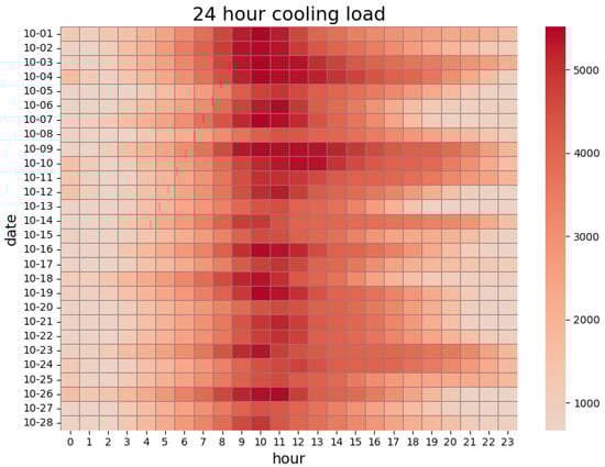
Figure 3.
Heat map of daily cooling load from 1 to 28 October 2024.
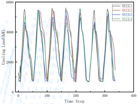
Figure 4.
The cooling load profiles over four consecutive weeks from 1 to 28 October 2024.
The heating map also highlights substantial nonlinearity and volatility in the cooling load. The intensity and width of peak-load regions vary from day to day, revealing the influence of fluctuating weather conditions, customer traffic, and operational schedules. For example, several days—such as October 5th, 12th, and 18th—show significantly intensified morning and afternoon load blocks, consistent with higher outdoor temperatures or increased weekend crowd flow.
As a large-scale commercial complex, the building experiences its highest cooling demand between 08:00 and 16:00, a period that largely overlaps with peak electricity pricing. Operating chillers directly during this interval would substantially increase operational costs. Introducing an ice-storage-based cooling strategy enables the system to shift load by producing ice during off-peak hours and releasing cooling energy during peak hours, thereby improving the overall COP and reducing cost.
Between 17:00 and 22:00, although outdoor temperatures gradually decrease, the commercial center enters another phase of high customer activity. This results in moderately high cooling demand, though with a generally declining trend compared with daytime peaks. From 23:00 to 08:00, most retail stores are closed, and the cooling requirement mainly comes from hotel and essential-service areas within the complex. During this period, the system primarily utilizes off-peak electricity for ice production, maintaining a relatively low and stable cooling load overnight.
To evaluate the predictive performance of the model, this study adopts three commonly used metrics: mean absolute error (MAE), root mean square error (RMSE), and the coefficient of determination (). MAE quantifies the average absolute difference between predicted and actual values, reflecting the overall forecasting error. RMSE, by computing the square root of the average squared differences, places greater emphasis on larger errors, making it suitable for assessing the performance of models on highly volatile time series. The metric measures the proportion of variance in the observed data that is explained by the model, ranging from , with values closer to 1 indicating better goodness-of-fit. The formulas for these metrics are as follows:
where and denote the actual and predicted values at the i-th time step, is the mean of the actual values, and n is the total number of samples. These evaluation metrics comprehensively reflect the magnitude of prediction errors and the model’s fitting quality, providing a solid basis for model comparison and performance assessment.
3.3. Experimental Design
All experiments were conducted on a single computing terminal equipped with an AMD Ryzen 7 6800H CPU, an NVIDIA GeForce RTX 3060 Laptop GPU, and 15.2 GB of RAM. Compared to large models such as Qwen2.5-3B and LLaMA-7B [23,26] commonly used in similar studies, this research adopts the relatively lightweight BERT-base model as the backbone network in order to achieve high timeliness in practical applications. As concluded from Table 3, although this choice sacrifices some prediction capacity, it significantly reduces computational costs without compromising prediction accuracy. During training, the Mean Squared Error (MSE) is used as the loss function to minimize prediction error, and the Adam optimizer [33] is employed for parameter updates. The dataset is split into training, validation, and testing sets with a ratio of 8:1:1. To avoid data leakage, normalization is performed solely based on the training set statistics. All experiments were independently repeated five times. For each run, predictions were made using the last model checkpoint, and the evaluation metrics were averaged across the five repetitions to ensure robust and reliable comparisons. Regarding the other hyperparameters, the rolling window size is set to 8 (4 h), the number of attention heads is set to 8, the embedding dimension is set to 16, and the feedforward network dimension is set to 32.
Several state-of-the-art models widely recognized in the field of time series forecasting are selected for comparative analysis with the ETime-LLM. Except for Time-LLM, Informer [34], a Transformer variant, incorporates a Prob-sparse self-attention mechanism to reduce computational complexity. TimesNet [35] adopts a modular design to decompose complex temporal variations across different periods and transforms the one-dimensional input series into two-dimensional representations, enabling unified modeling of patterns both inside and outside the time period. PatchTST [36] leverages a pure Transformer encoder, modeling time series as patch tokens without relying on recurrent or convolutional structures, thus achieving high modeling efficiency. DLinear [37], a lightweight multilayer perceptron (MLP)-based model, directly learns linear dependencies from decomposed series and performs well in tasks with limited long-term memory requirements. LightTS [38] employs a streamlined deep learning architecture with simplified feature extraction and modeling layers, enabling efficient large-scale time series forecasting. All models are implemented using the recommended settings provided in their respective publications to ensure optimal performance.
3.4. Long-Term Forecasting
To accurately regulate the total amount of ice storage during off-peak electricity pricing periods and avoid insufficient cooling or energy waste, it is essential for users to precisely forecast the time series of future cooling loads. In this section, considering the dataset’s sampling interval of 30 min, the input sequence length and output length is set to 48, corresponding to 24 h. This configuration ensures that the model has access to sufficient historical information for accurate prediction. The experimental results are presented in Table 4.
Table 4.
Forecasting results of cooling load for the next 24 h. The best values are highlighted in gray, while the second-best values are marked in dark red.
The experimental results demonstrate that the ETime-LLM algorithm outperforms all baseline models in terms of MAE, RMSE, and . The superior performance can be attributed to the synergistic integration of prompt-based modeling, cross-modal embedding, and reprogramming mechanisms. Specifically, prompt-based modeling constructs hierarchical prompts that incorporate task descriptions and statistical characteristics of the input sequence, effectively filtering redundant information and guiding the LLM to focus on relevant temporal patterns, especially the similarity-based lags and trend change localization derived from autocorrelation coefficients. Cross-modal embedding bridges the modality gap between continuous time series data and discrete language tokens by mapping segmented patches into the pre-trained token space of the LLM. The reprogramming mechanism enables efficient adaptation by freezing the parameters of the LLM, only training a lightweight reprogramming layer, thereby reducing computational cost and the risk of overfitting while preserving the model’s expressive power. Collectively, these components contribute to improved training efficiency and generalization capability in time series forecasting.
Figure 5 presents the hourly cooling load forecasts and corresponding residuals over 48 time steps (24 h) on the test set, further demonstrating the effectiveness of ETime-LLM in time series forecasting of cooling loads. By leveraging a prompt-based mechanism, the framework directs attention toward capturing anti-periodic fluctuations and non-noise trends embedded in the training data. This enables the model to better extract essential features and patterns within the cooling load sequences, especially the similarity-based lags and trend change localization derived from autocorrelation coefficients. The zoomed-in view in Figure 5 confirms that the ETime-LLM yields more stable residuals around inflection points compared to original version, demonstrating the effectiveness of the temporal enhancement mechanism. The residual curve further illustrates the distribution of prediction errors, confirming that ETime-LLM achieves higher forecasting accuracy and robustness by minimizing errors in cooling load forecasting.
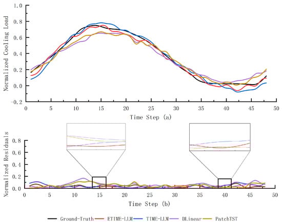
Figure 5.
A representative case of normalized hourly cooling load forecasting over the next 24 h is illustrated. Subfigure (a) shows the predicted curves generated by several comparison models, while subfigure (b) illustrates the corresponding residual curves.
3.5. Short-Term Forecasting
In HVAC systems, the short-term trajectory of future cooling load plays a critical role in determining the system’s response strategy, which in turn directly affects operational efficiency and energy consumption. Accurate short-term forecasting enables the system to deliver sufficient cooling capacity during peak demand periods while avoiding excessive cooling during low-demand intervals. Moreover, it allows the system to preemptively adjust such as by initiating pre-cooling or shutting down auxiliary components, based on anticipated load changes, thereby enhancing people comfort and reducing unnecessary equipment wear. In this section, we focus on short-term forecasting, with an input sequence length of 48 time steps and an output length of 4 time steps, corresponding to a 2 h forecasting horizon. The experimental results are summarized in Table 5, demonstrating the model’s capability to provide timely and reliable forecasts for dynamic load-responsive systems.
Table 5.
Forecasting results of cooling load for the next 2 h. The best values are highlighted in gray, while the second-best values are marked in dark red.
Although ETime-LLM demonstrates superior performance in long-term forecasting tasks, its performance slightly lags behind that of PatchTST in short-term load forecasting. This discrepancy can be attributed to several factors. First, PatchTST is specifically tailored for time series data, employing a patch tokenization mechanism directly on raw input, which is highly effective in capturing short-term local dynamics. In contrast, the prompt-driven inference in ETime-LLM relies on semantic reasoning and long-range dependencies, which may not provide significant benefits for short-term forecasting. Second, the high-dimensional semantic representations generated by the frozen language model in ETime-LLM may contain redundant information, introducing noise that adversely affects short-term accuracy. Figure 6 presents a concatenated curve of multiple 2 h ahead cooling load forecasting within the same day, illustrating the models’ capabilities in capturing temporal dynamics. It can be observed that at several turning points, ETime-LLM exhibits a slight delay in response. This may be attributed to its prompt-based semantic modeling mechanism, which is more adept at capturing global temporal structures rather than abrupt local fluctuations. Nevertheless, the overall trend alignment remains accurate, indicating that ETime-LLM effectively balances long-term contextual understanding with short-term forecasting accuracy.
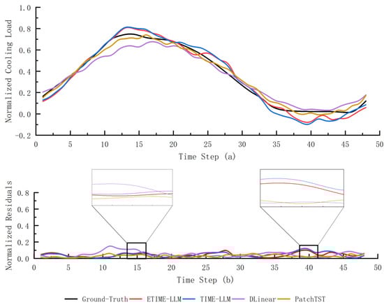
Figure 6.
An illustrative example of stitched 2 h forecast curves within a single day. Subfigure (a) shows the predicted curves generated by several comparison models, while subfigure (b) illustrates the corresponding residual curves.
3.6. Few-Shot Forecasting
Few-shot forecasting refers to the ability of a model to make accurate forecasts with only a small number of training examples or demonstrations. Unlike traditional deep learning approaches that rely on large-scale labeled datasets, ETime-LLM leverage prior knowledge acquired during pretraining to generalize to new tasks or domains with minimal supervision. In this section, we simulate real-world scenarios with limited training data availability by restricting the training set to 50% and 30% of the original samples. This setting evaluates the generalization capability and robustness of different models under few-shot forecasting conditions. In practical engineering applications, collecting and labeling large-scale time series data is often costly and time-consuming. Therefore, a model’s ability to perform well with only a small amount of training data is critical for its deployment in resource-constrained environments. The experimental results presented in Table 6 and Figure 7 and Figure 8 illustrate the relative performance of all models under reduced data conditions, as well as a representative forecasting example. The primary objective of the few-shot experiments is to evaluate the performance degradation caused by reduced training data, rather than to assess the stochastic stability of the models. Therefore, the standard deviations of the experimental results are not reported in this subsection.
Table 6.
Forecasting results for the next 24 h cooling load under few-shot scenarios. Results are shown for 50% and 30% training data. The best performance is highlighted in gray, and the second best is marked in dark red.
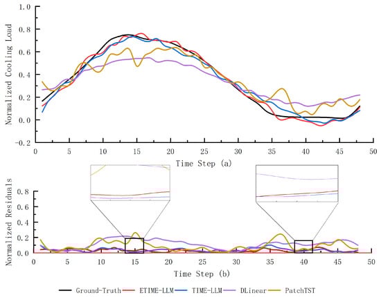
Figure 7.
An illustrates example of normalized hourly cooling load forecasting over the next 24 h under 30% data conditions. Subfigure (a) shows the predicted curves generated by several comparison models, while subfigure (b) illustrates the corresponding residual curves.
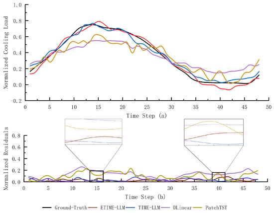
Figure 8.
An illustrates example of normalized hourly cooling load forecasting over the next 24 h under 50% data conditions. Subfigure (a) shows the predicted curves generated by several comparison models, while subfigure (b) illustrates the corresponding residual curves.
The experimental results also reveal some limitations. For instance, in the predicted results of the model trained with 30% of the dataset, Time-LLM exhibits a slight advantage over ETime-LLM at the inflection points. This phenomenon can be attributed to the fact that, in the 30% few-shot task, the FFT-based trend change detection module may extract misleading features when the data volume is small. For example, the FFT module in ETime-LLM assumes that changes in the cooling load are periodic, whereas, in reality, the inflection points of the cooling load are often influenced by external factors such as weather, which contradicts the periodicity assumption. These external factors may lead the model to extract biased nonlinear coupling relationships, causing the predicted inflection points to deviate from the actual curve.
3.7. Result Discussion
Across all long-term forecasting tasks, ETime-LLM consistently achieves the best performance when trained on both the full training set and the 30% subset, demonstrating its robustness and strong generalization capability under varying data availability. This suggests that the proposed enhancement mechanism is effective in leveraging the prior knowledge embedded in the frozen LLM and in extracting meaningful temporal patterns, even when only limited training samples are provided. Interestingly, Time-LLM attains the highest accuracy when trained on 50% of the data, although the performance gap between Time-LLM and ETime-LLM in this case remains small. One plausible explanation is that, under a moderate-data regime, the original Time-LLM architecture can already exploit a relatively rich set of temporal patterns, while the additional FFT-based trend prompting in ETime-LLM does not provide a clear advantage and may even introduce a mild mismatch between the periodicity assumption and the actual load dynamics.
In contrast, for short-term forecasting scenarios, PatchTST outperforms all other models, indicating its strength in capturing fine-grained local temporal dependencies over shorter horizons. This behavior is consistent with its design as a patch-based Transformer that focuses on high-resolution temporal segments, which is particularly beneficial when the forecasting term is short and the dynamics are dominated by local variations rather than long-range dependencies. By comparison, ETime-LLM and Time-LLM exhibit more pronounced advantages as the forecasting term becomes longer, where the ability to integrate prior knowledge and capture multi-scale temporal structures becomes increasingly important.
Overall, these results highlight the effectiveness of the proposed ETime-LLM framework while also revealing the trade-offs among different models under varying forecasting horizons and data regimes. ETime-LLM is better suited for long-term cooling load forecasting across a wide range of data availability settings, especially when sufficient historical information is accessible to support trend-aware prompting. Time-LLM remains a competitive alternative under moderate data conditions, and PatchTST stands out as a strong baseline for short-term forecasting where local temporal patterns dominate. These complementary characteristics suggest that, in practical applications, model selection or ensemble strategies could be tailored to the specific prediction horizon and data availability to achieve the best overall performance.
4. Conclusions
This study comprehensively validates the effectiveness of the ETime-LLM framework for time series forecasting of building cooling loads. By leveraging a frozen LLM as the backbone, ETime-LLM integrates prompt-based guidance, cross-modal embedding alignment, patch reprogramming, and an enhanced temporal feature mechanism to activate and steer the prior knowledge encoded in the LLM. This design enables deep modeling and high-precision prediction of complex temporal dynamics, particularly around trend transitions. To facilitate practical deployment, the framework adopts the lightweight and resource-efficient BERT-base model, which significantly lowers hardware requirements compared to larger LLMs such as LLaMA-7B and Qwen2.5-3B. This makes ETime-LLM well suited for computationally constrained edge devices in real-world engineering applications. Extensive experiments across long-term forecasting, short-term forecasting, and few-shot learning tasks demonstrate that ETime-LLM outperforms or matches state-of-the-art baselines in multiple evaluation metrics, in the commonly used 24 h forecasting horizon, compared with the original model, ETime-LLM achieves an approximately 17.3% reduction in MAE and a 19.3% reduction in RMSE. These results highlight its strong generalization capability, robust temporal sensitivity, and high potential for scalable deployment in intelligent, energy-efficient HVAC systems based on ice thermal energy storage.
In future work, the ETime-LLM framework could be further enhanced by integrating federated learning, enabling collaborative modeling across multiple distributed terminals while preserving data privacy. With this integration, local cooling load data collected at individual buildings can participate in model training without centralized data transmission, thereby mitigating privacy concerns, ensuring regulatory compliance, and improving the scalability and practicality of the framework in distributed building energy management.
Author Contributions
Conceptualization, C.Z. and Y.Y.; methodology, C.Z.; software, H.C.; validation, M.Z.; formal analysis, C.Z. and M.Z.; investigation, Y.Y. and H.C.; resources, H.C.; data curation, C.Z. and Y.Y.; writing—original draft preparation, C.Z.; writing—review and editing, Y.Y.; visualization, M.Z.; supervision, Y.Y.; project administration, H.C.; funding acquisition, H.C. and M.Z. All authors have read and agreed to the published version of the manuscript.
Funding
This research received no external funding.
Data Availability Statement
The original contributions presented in this study are included in the article. Further inquiries can be directed to the corresponding author.
Conflicts of Interest
Author Haiping Chen was employed by the company Contemporary Amperex Technology Co., Ltd. Author Miao Zeng was employed by the company Hangzhou RUNPAQ Environment & Engineering Co., Ltd. The remaining authors declare that the research was conducted in the absence of any commercial or financial relationships that could be construed as a potential conflict of interest.
Abbreviations
| ACO | Ant Colony Optimization |
| ANNs | artificial neural networks |
| COP | Coefficient of Performance |
| EERa | Energy Efficiency Ratio |
| FFT | Fast Fourier Transform |
| GCN | Graph Convolutional Networks |
| GRNs | Gated Residual Networks |
| HVAC | Heating, Ventilation, and Air Conditioning |
| IQR | interquartile range |
| LLM | large language model |
| MAE | mean absolute error |
| NLP | natural language processing |
| PaP | Prompt-as-Prefix |
| RMSE | root mean square error |
| RNNs | recurrent neural networks |
| TFT | Temporal Fusion Transformer |
| VSNs | Variable Selection Networks |
| WNN | Wavelet Neural Network |
References
- The State Council Information Office of the People’s Republic of China. China’s Energy Transition. 2024. Available online: http://www.scio.gov.cn/zfbps/zfbps_2279/202408/t20240829_860523.html (accessed on 30 June 2025).
- National Development and Reform Commission of the People’s Republic of China. Action Plan for Green and Efficient Refrigeration. 2019. Available online: https://www.ndrc.gov.cn/xxgk/zcfb/tz/201906/W020190905514433438027.pdf (accessed on 30 June 2025).
- Liu, X.; Lin, L.; Liu, X.; Zhang, T.; Rong, X.; Yang, L.; Xiong, D. Evaluation of air infiltration in a hub airport terminal: On-site measurement and numerical simulation. Build. Environ. 2018, 143, 163–177. [Google Scholar] [CrossRef]
- Sun, L.; Hu, Z.; Mae, M.; Imaizumi, T. Deep transfer learning strategy based on TimesBlock-CDAN for predicting thermal environment and air conditioner energy consumption in residential buildings. Appl. Energy 2025, 381, 125188. [Google Scholar] [CrossRef]
- Zou, M.; Huang, W.; Jin, J.; Hu, B.; Liu, Z. Deep spatio-temporal feature fusion learning for multi-step building cooling load forecasting. Energy Build. 2024, 1, 9. [Google Scholar] [CrossRef]
- Huang, X.; Zhou, X.; Yan, J.; Huang, X. Cooling load forecasting method for central air conditioning systems in manufacturing plants based on iTransformer-BiLSTM. Appl. Sci. 2025, 15, 5214. [Google Scholar] [CrossRef]
- Zhou, M.; Wang, L.; Hu, F.; Zhu, Z.; Zhang, Q.; Kong, W.; Zhou, G.; Wu, C.; Cui, E. ISSA-LSTM: A new data-driven method of heat load forecasting for building air conditioning. Energy Build. 2024, 321, 114698. [Google Scholar] [CrossRef]
- Hu, M.; Xiao, F.; Jørgensen, J.B.; Wang, S. Frequency control of air conditioners in response to real-time dynamic electricity prices in smart grids. Appl. Energy 2019, 242, 92–106. [Google Scholar] [CrossRef]
- Miller, J.A.; Aldosari, M.; Saeed, F.; Barna, N.H.; Rana, S.; Arpinar, I.B.; Liu, N. A survey of deep learning and foundation models for time series forecasting. arXiv 2024, arXiv:2401.13912. [Google Scholar] [CrossRef]
- Guo, H.; Xiao, G.; Su, L.; Zhou, J.; Wang, D.-H. Local neighbor propagation on graphs for mismatch removal. Inf. Sci. 2024, 653, 119749. [Google Scholar] [CrossRef]
- Huang, Y.; Li, C. Accurate heating, ventilation and air conditioning system load prediction for residential buildings using improved ant colony optimization and wavelet neural network. J. Build. Eng. 2021, 35, 101972. [Google Scholar] [CrossRef]
- Dong, F.; Yu, J.; Quan, W.; Xiang, Y.; Li, X.; Sun, F. Short-term building cooling load prediction model based on DwdAdam-ILSTM algorithm: A case study of a commercial building. Energy Build. 2022, 272, 112337. [Google Scholar] [CrossRef]
- Qu, Z.; Meng, Y.; Hou, X.; Chi, R.; Ai, Y.; Wu, Z. Integrated energy short-term multivariate load forecasting based on PatchTST secondary decoupling reconstruction for progressive layered extraction multi-task learning network. Expert Syst. Appl. 2025, 269, 126446. [Google Scholar] [CrossRef]
- Luo, Q.; Chen, Y.; Gong, C.; Lu, Y.; Cai, Y.; Ying, Y.; Liu, G. Research on Short-Term Air Conditioning Cooling Load Forecasting Based on Bidirectional LSTM. In Proceedings of the 2022 4th International Conference on Intelligent Control, Measurement and Signal Processing (ICMSP), Hangzhou, China, 8–10 July 2022; pp. 507–511. [Google Scholar] [CrossRef]
- Li, L.; Su, X.; Bi, X.; Lu, Y.; Sun, X. A novel Transformer-based network forecasting method for building cooling loads. Energy Build. 2023, 296, 113409. [Google Scholar] [CrossRef]
- Lim, B.; Arık, S.Ö.; Loeff, N.; Pfister, T. Temporal fusion transformers for interpretable multi-horizon time series forecasting. Int. J. Forecast. 2021, 37, 1748–1764. [Google Scholar] [CrossRef]
- Yu, D.; Liu, T.; Wang, K.; Li, K.; Mercangöz, M.; Zhao, J.; Lei, Y.; Zhao, R. Transformer based day-ahead cooling load forecasting of hub airport air-conditioning systems with thermal energy storage. Energy Build. 2024, 308, 114008. [Google Scholar] [CrossRef]
- Vanting, N.B.; Ma, Z.; Jørgensen, B.N. A scoping review of deep neural networks for electric load forecasting. Energy Inform. 2021, 4, 49. [Google Scholar] [CrossRef]
- Chen, W.; Liu, W.; Zheng, J.; Zhang, X. Leveraging large language model as news sentiment predictor in stock markets: A knowledge-enhanced strategy. Discov. Comput. 2025, 28, 74. [Google Scholar] [CrossRef]
- Chen, W.; Hussain, W.; Cauteruccio, F.; Zhang, X. Deep learning for financial time series prediction: A state-of-the-art review of standalone and hybrid models. Comput. Model. Eng. Sci. 2024, 139, 187–224. [Google Scholar] [CrossRef]
- Su, J.; Jiang, C.; Jin, X.; Qiao, Y.; Xiao, T.; Ma, H.; Wei, R.; Jing, Z.; Xu, J.; Lin, J. Large language models for forecasting and anomaly detection: A systematic literature review. arXiv 2024, arXiv:2402.10350. [Google Scholar] [CrossRef]
- Paroha, A.D.; Chotrani, A. A comparative analysis of TimeGPT and Time-LLM in predicting ESP maintenance needs in the oil and gas sector. Int. J. Comput. Appl. 2024, 186, 975–8887. [Google Scholar]
- Lin, H.; Yu, M. A novel distributed PV power forecasting approach based on Time-LLM. arXiv 2025, arXiv:2503.06216. [Google Scholar] [CrossRef]
- Ma, Y.; Lou, H.; Yan, M.; Sun, F.; Li, G. Spatio-temporal fusion graph convolutional network for traffic flow forecasting. Inf. Fusion 2024, 104, 102196. [Google Scholar] [CrossRef]
- Cen, S.; Lim, C.G. Multi-Task Learning of the PatchTCN-TST Model for Short-Term Multi-Load Energy Forecasting Considering Indoor Environments in a Smart Building. IEEE Access 2024, 12, 19553–19568. [Google Scholar] [CrossRef]
- Jin, M.; Wang, S.; Ma, L.; Chu, Z.; Zhang, J.Y.; Shi, X.; Chen, P.Y.; Liang, Y.; Li, Y.F.; Pan, S.; et al. Time-LLM: Time series forecasting by reprogramming large language models. In Proceedings of the International Conference on Learning Representations (ICLR), Vienna, Austria, 7–11 May 2024. [Google Scholar]
- Devlin, J.; Chang, M.; Lee, K.; Toutanova, K. BERT: Pre-training of Deep Bidirectional Transformers for Language Understanding. arXiv 2018, arXiv:1810.04805. [Google Scholar]
- Jiang, Y.; Sun, W. Day-Ahead Electricity Price Prediction and Error Correction Method Based on Feature Construction–Singular Spectrum Analysis–Long Short-Term Memory. Energies 2025, 18, 919. [Google Scholar] [CrossRef]
- Xu, J.; Guo, Z.; He, J.; Hu, H.; He, T.; Bai, S.; Chen, K.; Wang, J.; Fan, Y.; Dang, K.; et al. Qwen2.5-Omni Technical Report. arXiv 2025, arXiv:2503.20215. [Google Scholar] [CrossRef]
- Touvron, H.; Lavril, T.; Izacard, G.; Martinet, X.; Lachaux, M.A.; Lacroix, T.; Rozière, B.; Goyal, N.; Hambro, E.; Azhar, F. Llama: Open and efficient foundation language models. arXiv 2023, arXiv:2302.13971. [Google Scholar] [CrossRef]
- Radford, A.; Wu, J.; Child, R.; Luan, D.; Amodei, D.; Sutskever, I. Language models are unsupervised multitask learners. OpenAI Blog 2019, 1, 9. [Google Scholar]
- Zhou, J.; Yao, Y.; Chen, X.; Guo, H.; Li, Q.; Deng, Z. Triplet relationship guided density clustering for feature matching with a large number of outliers. Clust. Comput. 2025, 28, 1–15. [Google Scholar] [CrossRef]
- Kingma, D.P.; Ba, J. Adam: A method for stochastic optimization. arXiv 2014, arXiv:1412.6980. [Google Scholar]
- Zhou, H.; Zhang, S.; Peng, J.; Zhang, S.; Li, J.; Xiong, H.; Zhang, W. Informer: Beyond efficient transformer for long sequence time-series forecasting. In Proceedings of the AAAI Conference on Artificial Intelligence, Virtual, 19–21 May 2021; Volume 35, pp. 11106–11115. [Google Scholar]
- Wu, H.; Hu, T.; Liu, Y.; Zhou, H.; Wang, J.; Long, M. Timesnet: Temporal 2d-variation modeling for general time series analysis. arXiv 2022, arXiv:2210.02186. [Google Scholar]
- Nie, Y.; Nguyen, N.H.; Sinthong, P.; Kalagnanam, J. A time series is worth 64 words: Long-term forecasting with transformers. arXiv 2022, arXiv:2211.14730. [Google Scholar]
- Zeng, A.; Chen, M.; Zhang, L.; Xu, Q. Are transformers effective for time series forecasting? In Proceedings of the AAAI Conference on Artificial Intelligence, Washington, DC, USA, 7–14 February 2023; Volume 37, pp. 11121–11128. [Google Scholar]
- Zhang, T.; Zhang, Y.; Cao, W.; Bian, J.; Yi, X.; Zheng, S.; Li, J. Less is more: Fast multivariate time series forecasting with light sampling-oriented mlp structures. arXiv 2022, arXiv:2207.01186. [Google Scholar] [CrossRef]


Disclaimer/Publisher’s Note: The statements, opinions and data contained in all publications are solely those of the individual author(s) and contributor(s) and not of MDPI and/or the editor(s). MDPI and/or the editor(s) disclaim responsibility for any injury to people or property resulting from any ideas, methods, instructions or products referred to in the content. |
© 2025 by the authors. Licensee MDPI, Basel, Switzerland. This article is an open access article distributed under the terms and conditions of the Creative Commons Attribution (CC BY) license (https://creativecommons.org/licenses/by/4.0/).