Abstract
This study proposes Bayesian estimation of multivariate regular vine (R-vine) copula models with generalized autoregressive conditional heteroskedasticity (GARCH) margins modeled by Gaussian-mixture distributions. The Bayesian estimation approach includes Markov chain Monte Carlo and variational Bayes with data augmentation. Although R-vines typically involve computationally intensive procedures limiting their practical use, we address this challenge through parallel computing techniques. To demonstrate our approach, we employ thirteen bivariate copula families within an R-vine pair-copula construction, applied to a large number of marginal distributions. The margins are modeled as exponential-type GARCH processes with intertemporal capital asset pricing specifications, using a mixture of Gaussian and generalized Pareto distributions. Results from an empirical study involving 100 financial returns confirm the effectiveness of our approach.
Keywords:
regular vine copulas; variational bayes with data augmentation; exponential-type generalised autoregressive conditional heteroskedasticity model; intertemporal capital asset pricing model; mixture distribution; Markov chain Monte Carlo MSC:
62E; 62F; 62H; 62J
1. Introduction
Over the past few decades, following the work of [1], who demonstrated that copula functions can capture non-linear comovement between variables, research on copula-based dependence structure models has grown rapidly. One of the key advantages of copulas, as multivariate distribution tools, is their ability to link different marginal distributions. As a result, copulas have been widely applied across various fields, including hydrology [2], energy [3], agricultural and forest meteorology [4], oceanology [5], computer science [6], insurance [7], and more widely in economics and finance [8,9].
A substantial body of literature demonstrates that copula models, particularly due to their ability to capture tail asymmetry, are highly effective for modeling dependence in quantitative risk management. Tail modeling plays a crucial role in risk assessment, where common measures include Value-at-Risk (VaR) and Conditional Value-at-Risk (CVaR), also known as expected shortfall. For formal definitions of risk measures, see [10]. Among multivariate dependence models, standard copulas are widely used. These typically fall into two main families: elliptical and Archimedean copulas (see [11,12,13,14] for details). However, standard multivariate copulas come with certain limitations—most notably, they rely on a single parameter to govern all pairwise tail dependencies. This becomes problematic in high-dimensional settings, where such a simplification can be unrealistic. This limitation was identified by [15], who introduced a more flexible class of models known as regular vine (R-vine) copulas. Two notable subclasses within the vine copula framework are the canonical vine (C-vine) and the drawable vine (D-vine) copulas [16]. Further discussion on vine copulas can be found in Section 2, and additional details are provided in Chapter 3 of [17].
It consists of two copula families: one is elliptical copulas—see Wichitaksorn et al. [11], Liang and Rosen [13] for recent studies—and the other is Archimedean copulas; see Michaelides et al. [14] and Górecki et al. [12] for recent studies.
In the existing literature, research on vine copulas—particularly R-vines—remains relatively limited. This is likely due to their structural complexity and the intensive computational effort required. Specifically, R-vines allow for a significantly larger number of possible tree structures compared to C-vines and D-vines, especially as the dimensionality increases. Despite these challenges, R-vines offer considerable flexibility as dependence models. Their wide range of possible structures makes them highly adaptable, and importantly, they overcome the parameter limitation of standard multivariate copulas. This added flexibility is particularly advantageous for analyzing tail dependence in high-dimensional financial data.
To our knowledge, there are few studies in the financial literature on R-vines with high dimensions. For instance, ref. [18] studied up to 398 dimensions on S&P500 constituents and ref. [19] studied 2131 dimensions, while other R-vine studies have examined the lower dimensions (less than 25). See, among others, the studies of R-vines in lower dimensions in [20,21,22,23,24,25]. For studies on copula models, see, among others, [26,27,28,29]. Hence, the study of R-vines in high dimensions is still scarce and needs more investigation. This observation is the starting point of our study. The model most closely related to ours is that of [30], which studies R-vines in application to 16-dimensional financial indices using the quasi-maximum likelihood estimation (QMLE) method.
Given standardized residuals, vine copula models can be applied across five different classes: mixed R-vines, mixed C-vines, mixed D-vines, all-t R-vines, and the standard multivariate Gaussian copula. This study utilizes seven bivariate copula families. Based on the test proposed by [31] and likelihood comparisons, previous research has identified mixed R-vines as the best-performing models—an approach we adopt in this study.
Our first contribution is to extend this analysis to 100 dimensions of financial data using constituents of the S&P500, which, to our knowledge, has not been explored in this context. The second contribution is the expansion of the copula family set from seven to thirteen bivariate copulas, including two-parameter BB families and additional Archimedean copulas. This broader selection allows for a more accurate capture of tail asymmetries observed in financial data. Further details are provided in Section 4. Our third contribution lies in the modeling of the marginal distributions. We employ the intertemporal capital asset pricing model (ICAPM), originally proposed by [32], with an asymmetric GARCH model featuring a mixture innovation. This approach enhances the filtration of volatility clustering and yields deeper insights into risk premia across individual financial returns. Unlike [30], who used an ARMA-GARCH model with a single Student-t innovation, we incorporate a mixture of one Gaussian and two heavy-tailed distributions, offering a more flexible representation of return dynamics.
Another key contribution of this study lies in the estimation methodology. In the existing literature, quasi-maximum likelihood estimation (QMLE) is widely used for copula models; see, for example, [33,34,35]. However, QMLE has notable limitations—it is highly sensitive to initial parameter values and often suffers from convergence issues [36]. To address these shortcomings, we employ more efficient estimation techniques, specifically Bayesian Markov chain Monte Carlo (MCMC) and variational Bayes (considered as machine learning) methods, to estimate our proposed R-vine dependence models. These methods are also compatible with the two main subclasses of vine copulas: C-vines and D-vines. While Bayesian MCMC and machine learning approaches are computationally intensive, we mitigate the associated costs by incorporating parallel computing. Additionally, we use QMLE estimates as initial values to improve convergence speed in the Bayesian MCMC and machine learning algorithms.
Our study explores these advanced methods in two distinct ways. First, we apply the random walk Metropolis–Hastings (rw-MH) algorithm for Bayesian MCMC estimation. Second, we implement the variational Bayes method—both with and without data augmentation (VBDA)—as proposed by [37], to estimate the multivariate dependence structure. Furthermore, we propose an alternative, more efficient variational approximation to reduce computational time, the details of which are presented in the simulation study in the Supplementary Material. For related surveys on MLE, Bayesian, and machine learning methods, see [38,39,40,41], among others.
The remainder of the paper is structured as follows. Section 2 introduces the graph-theoretical framework for high-dimensional regular vine (R-vine) copulas, including the two special subclasses—C-vines and D-vines—as well as the marginal models. Section 3 outlines the Bayesian inference and machine learning algorithms used to estimate general R-vine dependence models. Section 4 presents empirical results based on 100-dimensional financial data. Section 5 offers concluding remarks. Details on the simulation study and data generation algorithms are provided in the Supplementary Material.
2. Graph Theory
2.1. Regular Vines in n-by-n Matrix Representation
This section provides the theoretical background on regular vine (R-vine) copulas, along with two important subclasses: canonical vine (C-vine) and drawable vine (D-vine) copulas, all represented in an n-dimensional graphical model framework. In graph theory, an R-vine is represented as a sequence of tree structures composed of nodes N and edges E. An R-vine () in n-dimensions is defined as a nested set of trees. The first tree () consists of n nodes and edges, each representing a pair of variables. Each edge in becomes a node in the second tree (), which then has nodes and edges. The construction follows the proximity condition, meaning that connected nodes in must share a common node from .
This nesting continues: in the third tree (), there are nodes and edges, and again, any two connected nodes must share a common node from . This process continues until the final tree (), which has two nodes and a single edge. These two nodes must share all remaining nodes from the previous tree. For further definitions and examples—including complete unions, conditioning sets, and conditional sets of an edge—refer to [30]. Additional theoretical details and properties of vine copulas can be found in [17,42,43,44].
A convenient approach for developing an algorithm in a vine graphical model is to store the trees in an n-by-n matrix. The authors of [30] proposed using a lower triangular matrix to represent vines as a tree structure in n dimensions; see Figure 1.
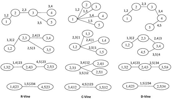
Figure 1.
An illustrative example of vine copula graphical model in five dimensions.
Definition 1
(Matrix Constraint Set). Let be a lower triangular n-by-n matrix where . The constraint set for is
for . Otherwise, (if ). Hence, is the conditioning set and is the conditioned set.
In other words, every pair variable within the constraint set is built up from a diagonal element plus another element in the same column conditioning on set of . Otherwise, when i equal to n. To illustrate Definition 1, the 5-by-5 matrix of Figure 1 can be constructed as
Once a 5-by-5 matrix is constructed, it becomes straightforward to generalize the construction to an matrix for any dimension n. For different constructions of upper triangular matrices representing vines in graphical theory, see [17] (Chapter 3).
2.2. Multivariate Regular Vines Density
This section introduces the matrix within a numerical framework for computing multivariate regular vine copula densities, including both multivariate canonical vine (C-vine) and drawable vine (D-vine) structures in n-dimensions. In the previous section, we generated an n-by-n matrix satisfying a proximity condition. Building on this, the n-dimensional multivariate vine copula density is now formulated using two additional n-by-n matrices: the bivariate copula type matrix and its associated parameter matrix where and .
We begin by expressing the vine copula density as a product of pairwise copula functions. According to Sklar’s theorem, a copula C is a multivariate distribution function that links a joint distribution to its marginals [1]. Thus, the multivariate copula distribution can be written as:
for n-dimensional data. After that, vine copula density in n-dimensions can be expressed in graph theory. In product indexing, the C-vine density is
The D-vine density is
The R-vine density is
In a D-vine, each node in a given tree can be connected to only one edge. In contrast, within a C-vine, a specific node in tree must have edges. The D-vine structure allows for more independence assumptions compared to the C-vine. However, the C-vine can be advantageous when there is prior knowledge of a particular variable that strongly influences the dataset. The R-vine represents the most general form, offering significantly greater flexibility in modeling complex dependency structures.
Figure 1 provides an example of a five-dimensional regular vine copula density. The complete R-vine copula density depicted in this figure can be expressed as follows:
where stands for . All definitions and further details can be found, among others, in [15] for C-vines and D-vines, and in [30] for R-vines. Next, we present R-vine density using matrix representation , , and in Figure 2, which can be used for its special cases.
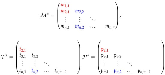
Figure 2.
Vine copula specification in n-by-n matrix representation including , and .
In Figure 2, the red label corresponds to the last tree, . The conditioned set is , and the conditioning set includes all elements . The associated bivariate copula type and parameter are and , respectively.
The blue label represents the first tree, . Here, the conditioned set is , and the conditioning set is ∅. The corresponding bivariate copula type and parameter are and , respectively.
2.3. Marginal Model and Distribution
This section presents our proposed marginal model, which combines elements of the ICAPM and an asymmetric GARCH model with a mixture distribution. This hybrid approach is designed to capture key stylized facts of financial returns, such as volatility clustering and time-varying heteroskedasticity. The model offers several advantages, including the incorporation of risk premium information and the ability to account for asymmetric shocks and fat-tailed behavior in financial data.
Our marginal model is similar to that of [45], who employed Gaussian innovations; however, we adopt a more flexible mixture innovation to better reflect the complexity of financial return distributions. Furthermore, we extend this framework to the multivariate setting in order to analyze dependence structures using regular vine copulas.
The ICAPM we use in this study follows [32], which is a linear-in-variance function of financial returns and is given by
where is the financial returns at time , is a risk-free rate, is a risk premium, is a conditional volatility, is an innovation with zero mean and the conditional variance (or volatility) , and is the independent and identically distributed (iid) random variable with zero mean and unit variance from a mixture distribution. To deal with the heteroskedastic returns, we use an exponential-type GARCH model or EGARCH(p,q,r) given by
where is a constant, measures the direct innovation effects, is the asymmetry parameter for the leverage effects, and is the volatility persistence parameter. For details on the EGARCH model, see [46], as well as the surveys on asymmetric GARCH models, including EGARCH, in [47,48]. Regarding the distribution of innovations in the marginal model, we employ a mixture distribution originally proposed by [49] for use with the ARMA-GARCH model and standard copulas. In contrast, our study applies this mixture distribution within an ICAPM-EGARCH framework combined with regular vine copulas.
The mixture distribution consists of three components: one Gaussian distribution and two generalized Pareto distributions (GPDs) derived from extreme value theory (EVT). The GPD components are specifically designed to capture asymmetric fat tails—one of the most significant features observed in financial return data [50].
The mixture distribution has a flexible property. It can be represented by either a finite set of distribution functions (cdf), , or density functions (pdf), , . The mixture distribution and its density are a weighted sum such that and , respectively. is a weight and . If the mixing weight w is pre-specified, it can also represent the quantile level of the mixture distribution. Given the three components, the mixture pdf is given by
where and are a pre-specified quantile, is a location parameter, is a scale parameter, is a shape parameter, and L and R denote the left and right tails, respectively. The support of is when and when , and represents a fat tail and exists at least up to the second moment. For more details on the moment property, see [51,52].
The GPDs, in a sense of generalization, consist of an ordinary Pareto distribution, an exponential distribution, and a short-tailed, Pareto type II distribution. Further details of the GPD used in the peak-over-threshold method are found in ([10] Chapter 5). Note that and are the standard Gaussian pdf and its inverse cdf, respectively.
3. Bayesian Inference and Machine Learning in the Graphical Model
This section outlines the parameter estimation techniques used in our study, which include both Bayesian and machine learning approaches. For the Bayesian framework here, we refer to the Markov chain Monte Carlo (MCMC), while the variational Bayes is considered a machine learning method. Though both methods are computationally demanding and mathematically intricate, they are well-suited for cases where the posterior distribution of the marginal models is intractable—as is the case in our analysis.
Specifically, we apply the random walk Metropolis–Hastings (rw-MH) MCMC algorithm proposed by [53], along with the variational Bayes method developed by [37], both with and without data augmentation. These methods are used to estimate model parameters and to analyze the R-vine copula dependence structure.
To support and enhance the efficiency of these estimation procedures, we also incorporate plug-in parallel computing and the quasi-maximum likelihood estimation (QMLE) method. These additions help reduce computational time while preserving estimation accuracy, thereby facilitating the integration of Bayesian inference and machine learning techniques in a computationally feasible manner.
3.1. Full Likelihood Function
It is important to first discuss a likelihood function since this is a connection between Bayesian MCMC and machine learning methods. Given the observed n-dimensional data, the full log-likelihood function of our model is
where
which is compatible with Equation (4). is a unique bivariate copula pdf. is a mixture cdf which is defined in Section 2.3. is a standardized residual given by Equation (5). The parameter in parameter space is . In n dimensions, there are at least parameters that need to be estimated. The number of parameters grows proportionally to the number of dimensions. From our R-vine copula-based models, there are at least 606 parameters in 30 dimensions and 6094 parameters in 100 dimensions, respectively. Notably, the trade-off between flexibility and parsimony needs to be taken into account. This leads to a research area of regularization or shrinkage method where the most common shrinkage methods are, for instance, lasso and ridge—see [54,55,56], among others. However, we leave this for further research.
3.2. Bayesian MCMC Estimation
Due to the intractable nature of the likelihood, a Bayesian approach is a good candidate for the estimation. Hence, this section discusses the rw-MH algorithm, enhanced with the QMLE and parallel computing to improve computational efficiency. Given the large number of parameters in vine copula models, we adopt the Inference for Margins (IFM) approach [57], which enables the parallelization of marginal model estimation and significantly accelerates the overall computation. Regarding the choice of prior distributions, we use an informative prior, especially the uniform distribution, in the estimation with the hyperparameter values following previous studies.
In summary, Algorithm 1 outlines the procedure for obtaining the parameter estimates for the R-vine copula model and for the marginal models. The process begins by constructing the maximum matrix from , where each element in represents the maximum value among all entries in the k-th column from row i to row n.
The algorithm proceeds in several parallelized steps. The first loop performs data standardization in parallel. In the second loop, the algorithm computes the independent pairwise copulas in the first tree, , of the R-vine model—also in parallel. The third loop handles the dependent pairs in the subsequent trees , for .
| Algorithm 1 Parallel algorithm of regular vine copulas model using random walk chain Metropolis–Hastings sampling MCMC and maximum likelihood estimation. |
|
To ensure better convergence, the algorithm initially employs the QMLE to provide starting values for the rw-MH sampler, described in Algorithm 2, which functions as a subroutine within Algorithm 1.
The function denotes a specific bivariate copula density, parameterized by copula type t and parameter . The terms and refer to recursive conditional cumulative distribution functions (cdfs), often denoted by , which are fundamental components in the construction of conditional copulas in vine structures.
for all . Denote that . where is a bivariate survival function and are monotonically decreasing transforms. Therefore, the conditional cdf is See [30] for further discussion.
Algorithm 2 presents the rw-MH sampling method used as part of the MCMC procedure in Algorithm 1. In general, the performance of the Metropolis–Hastings algorithms is sensitive to the choice of initial values () where is a covariance matrix. The first stage of the rw-MH algorithm involves a burn-in period, during which early samples of are discarded. A longer burn-in period increases computational time, and its length largely depends on how close the initial values are to the target distribution.
To address this, our approach initializes the algorithm with parameter estimates obtained via the QMLE. This helps achieve a reasonable acceptance rate more quickly— approximately 50% in our implementation.
The proposal step involves an increment random variable z, which follows a Gaussian distribution, , where c is a constant scaling factor. This constant is tuned to ensure an appropriate acceptance rate for the sampler. For further details on the MH algorithm, see [53] (Exercise 17.5 and Exercise 11.18).
| Algorithm 2 Random walk Metropolis–Hastings algorithm |
|
3.3. Variational Bayes Estimation
This section introduces an alternative algorithm based on the variational Bayes (VB) method, which integrates Bayesian inference with machine learning to estimate n-dimensional general regular vine copula models. Specifically, we apply the variational Bayes with (and without) data augmentation (VBDA) approach originally developed for a drawable vine structure by [37,58].
In this study, we extend the VBDA method to accommodate the more general class of regular vines by incorporating an additional stopping criterion. This enhancement is designed to reduce the number of iterative learning steps, thereby improving computational efficiency.
We explore three versions of the variational Bayes estimation method: one without data augmentation (VBDA0), and two with data augmentation (VBDA1 and VBDA2). All three methods rely on latent variables during estimation. To address convergence challenges and reduce computational time, we also incorporate plug-in QMLE estimates and leverage parallel computing techniques.
The augmented posterior density is
where is the prior density. is the marginal likelihood function. is the copula density. is the indicator function. VB estimation approximates by a tractable density in a so-called variational approximation. This estimation corresponds to minimizing the Kullback–Leibler (KL) divergence
or maximizing the lower bound of the logarithm of the marginal likelihood (or the evidence lower bound (ELBO)), given by
where and are independent. For further details and examples of VB methods, see, among others, [59,60]. Also, see [61,62], among others, for reviews of VB inference in machine learning.
The density approximation of can be written as . The specification of and is crucial. has parameter while has parameter with the support on . This study selects the choice of approximation as follows:
VBDA2 nests VBDA1, which covers a wide range of data dependencies with an effective mean field approximation. VBDA1 is expected to be more accurate for data with low dependence. , , and is the standard normal density.
To approximate , we adopt a commonly used variational distribution , specifically the multivariate normal (Gaussian) distribution with mean M and covariance matrix , denoted as . In the context of R-vine models, a large number of parameter estimates are required. The use of a tractable multivariate normal distribution makes it relatively straightforward to compute the gradient of .
Moreover, the structure of contributes to improving the accuracy of the gradient estimates. In particular, when is expressed using its factorized form , the gradient of this factorization has been derived and shown to be computationally efficient [63].
Algorithm 3 shows the VBDA algorithm with stochastic gradient ascent optimization. Note that, in Algorithm 1, Algorithm 2 is replaced by Algorithm 3 in order to perform VBDA method in the R-vine model. This approach is tractable posterior distribution.
| Algorithm 3 Variational Bayes data augmentation with control variates and ADADELTA learning rate |
|
A brief overview of the procedure is as follows:
Three VB estimators for regular vine dependence models are introduced in Line 4, where the specification of can be one of DA0, DA1, or DA2. To initiate the algorithm, an initial value for the variational parameter, , is required, typically initialized using QMLE estimates .
In Line 12, the lower bound (LB) is updated iteratively as follows: . Here, is the learning rate, and is an unbiased estimate of the gradient of the lower bound , computed using the ADADELTA optimization method (Line 11). For further details on adaptive learning rate techniques like ADADELTA, see [64].
The gradient of the lower bound, , is expressed as the expectation:
where represents the unnormalized posterior distribution.
To reduce the variance of this unbiased gradient estimator, a control variate vector is employed. Consequently, the unbiased estimator of the gradient is given by where where and m is the number of elements in , and SS is the number of Monte Carlo samples.
For a more detailed discussion of the VBDA algorithm, refer to [30] (Section 3).
The stopping rule for the algorithm terminates the iterative procedure if
- (i.)
- There is a fixed number of stochastic gradient ascent steps, , or
- (ii.)
- The moving average is not improved, , which is referred to as the parameter and in Line 20 and the whole procedure stops when maximum patience P in Line 22–23, and
- (iii.)
- All of the above conditions will be checked when the iteration is greater than a constant c.
Finally, is collected when is greater than [60]. Note that the simulation study in Bayesian inference and machine learning including the rw-MH algorithm and the VBDA algorithm can be found in the Supplementary Material. The results show that, in general, the VB methods perform better than the others.
4. Empirical Study
4.1. Data
This study analyzes financial market time series data with up to 100 dimensions. For the training set, we selected the daily adjusted closing prices of the top 100 Nasdaq-listed stocks by market capitalization, covering the period from 2 January 2009 to 20 September 2021, where we intentionally avoided the impact of the 2008 global financial crisis. Only stocks listed before 2009 were included, resulting in a total of 3201 daily observations. The test set spans from 21 September 2021 to 21 December 2021, comprising 65 daily observations. All data were obtained from Yahoo Finance using MATLAB 2022a’s data feed function. The experiments were implemented in MATLAB and conducted on a laptop equipped with an 11th Gen Intel(R) Core(TM) i7-1185G7 processor (3.00 GHz) and 32 GB of RAM.
After completing data cleaning, we obtained 100 stock indices for use in our empirical study. A full list of these indices is provided in Appendix C. To evaluate the performance of the proposed models described in Section 2, we conducted two empirical experiments using two datasets: one consisting of all 100 time series and another with only the last 30 stock indices. The goal of these experiments was to assess the scalability and effectiveness of the proposed model as the dimensionality increases.
The descriptive statistics of the dataset are summarized as follows. The top five business sectors represented in our analysis are technology (22 firms), health care (18 firms), finance (11 firms), consumer services (11 firms), and capital goods (8 firms). The total market capitalization of the selected stocks is USD 30,814 billion, accounting for approximately 46% of the total market capitalization on the Nasdaq exchange.
All stocks exhibit a positive mean return, with return values ranging from −39.02% to 52.29%. The standard deviation ranges from 1.06% to 3.67%, while skewness values range between −1.04 and 1.56. Kurtosis spans from 5.95 to 47.26. These statistics indicate that the return distributions are asymmetric and exhibit heavy tails.
Additionally, the Jarque–Bera test statistics for all returns strongly reject the null hypothesis of normality at the 1% significance level, confirming that the return distributions deviate significantly from normality.
4.2. Regular Vine Distribution Selection
Multivariate copula models can be fitted to n-dimensional time series data using a two-stage sequential approach [30]. In the first stage, a univariate marginal model is selected and fitted separately to each time series to obtain standardized residuals, which are then transformed into marginally uniform variables. In this study, we apply our proposed marginal model, detailed in Section 2.3, and compare its performance to a widely used benchmark: the ARMA(1,1)-GARCH(1,1) model with Student-t innovations.
In the second stage, the dependence structure among the transformed residuals is modeled using a multivariate copula. It is well established in the literature that different pairs of financial variables exhibit varying degrees of asymmetry and tail dependence. Traditional multivariate copulas are generally unable to capture such heterogeneous dependence structures. Vine copulas, however, are specifically designed to address this limitation.
While D-vine and C-vine copulas are effective in modeling complex dependencies, they are constrained by their predefined path structures. To overcome this limitation, we investigate the use of regular vine (R-vine) copulas—a more flexible and general class that encompasses both D-vines and C-vines as special cases. R-vines offer significantly greater modeling capacity due to their extensive variety of possible tree structures and pair-copula combinations.
In fact, for high-dimensional datasets, the number of possible R-vine structures grows rapidly, with the total number given by [65], underscoring their flexibility and complexity compared to standard copula models and their vine subclasses.
The following tasks are the sequential steps of fitting an R-vine copula with marginal specification:
- (a)
- Standardize the residuals of the returns using the univariate marginal model.
- (b)
- Select the R-vine path structure of the tree, , given by maximized empirical via
- b.1
- Formulation of empirical of all possible pairs variable, , ;
- b.2
- Performing the spanning tree maximization (the sum of absolute empirical )
- b.3
- For each edge, selection of bivariate copula family and its parameter(s) from all possible bivariate copula candidates via Bayesian information criterion (BIC) value.
- (c)
- Iterate Step (b) from the first tree (unconditional tree, ) to the last tree (conditional tree, where D is the proximity condition).
The methodology described above yields a complete specification of a regular vine copula, including . The QMLE is employed in Step b.3 to estimate all relevant parameters. This full specification is then used as the foundation for our Bayesian inference and machine learning procedures.
It is important to note that, for the first tree in the vine structure, parallel computation is feasible due to the independence of the path structure in R-vines. The method proceeds as follows:
- Step 1 (Tree 1): A parallel computation technique is applied to estimate for .
- Step 2: A FOR loop is used to compute where .
For more details on the maximum spanning tree algorithm used in this context, see [30].
Our study employs a range of bivariate copula functions to capture the diverse (a)symmetrical dependence structures present in financial time series data. While the core families considered include the Gaussian, Student-t, Gumbel, and Frank copulas—consistent with the approach of [30]—we extend the analysis by incorporating a total of 13 copula families. The complete list of candidate bivariate copula families used in this study is provided below:
- Gaussian/Normal copula presents symmetric and no tail dependence.
- Student-t copula presents symmetric and upper and lower tail dependence.
- Frank copula presents symmetric and tail independence.
- Clayton copula presents asymmetric and lower tail dependence.
- B5/Joe, Gumbel, and Galambos copulas present asymmetric and different upper and lower tail dependence.
- BB1, BB3, BB4, BB5, BB7 and BB10 copulas present asymmetric and different upper and lower tail dependence.
Details of the bivariate copula distributions and their key dependence structure properties are summarized in Appendix A. These include the cumulative distribution functions, lower and upper tail dependence orders, and rank-based dependence measures. For additional discussion on copula properties, see, among others, [17] (Chapter 4) and [66] (Appendix).
We also conducted Ljung–Box tests on the standardized residuals from all proposed models. The results confirm the independence of the residuals. Full details of these tests are provided in Appendix B.
4.3. Empirical Results
In this section, we present the empirical results obtained from our proposed Bayesian models and estimation methods for R-vine copulas. A comprehensive set of 13 bivariate copula families is employed within the regular vine structure to capture complex dependence patterns.
For the univariate margins, we apply the mixture distribution defined in Equation (7) to the ICAPM-EGARCH models, which are designed to capture key features of financial time series data such as volatility clustering and heavy tails.
As a benchmark, we use the traditional QMLE method and compare its performance with our proposed approaches, including the rw-MH algorithm and the VBDA methods. These methods are implemented in the R-vine copula framework for dimensions of up to 100. In total, the empirical study involves the estimation of up to 4950 bivariate copula functions and 6138 parameters.
The experimental results, summarized in Table 1 and Table 2, indicate that the VBDA1 method delivers the best performance in terms of marginal likelihood on the training set. On the test set, the variational Bayes approaches—particularly VBDA1—demonstrate substantial improvements in forecasting accuracy as the dimensionality increases, making them strong candidates for high-dimensional modeling. Specifically, as both the number of dimensions and the forecast horizon grow, VBDA1 provides more accurate variability estimates. In contrast, the QMLE method performs relatively poor in higher dimensions and longer forecast horizons. However, in the case of 30 dimensions with a three-month forecast window, QMLE outperforms the other methods.

Table 1.
Performance comparison of 30 dimensions.
Table 2.
Performance comparison of 100 dimensions.
For 100-dimensional data, VBDA1 achieves the best forecasting performance based on the mean absolute deviation (MAD). Meanwhile, both the rw-MH and QMLE methods yield the best performance in terms of root mean square error (RMSE) for the three-month test set, while rw-MH shows the strongest performance in one-month forecasts at the 100-dimensional level.
Figure 3 illustrates a representative example of the empirical results for a normalized R-vine copula contour plot and rank-based dependence measures. These results are based on the univariate ICAPM-EGARCH–mixture marginal model using the VBDA2 estimation method in a 30-dimensional setting.
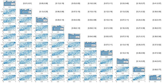
Figure 3.
Estimation results of normalized mixed R-vine copula contour plot, Kendall’s , and Spearman’s for 10 stock indices in the 30-dimensional cases using R-vine–ICAPM–EGARCH–Mixture model and VBDA2 method. Notes: Due to space, only 10 representative stocks are shown. Contour plots are shown in the lower triangular matrix while [Kendall’s , Spearman’s ] are shown in the upper triangular matrix.
Due to space, we present a normalized 10-dimensional subset of the R-vine contour plot for selected stock indices. The stock names appear along the diagonal of the matrix. The lower triangular part of the matrix displays the R-vine copula contours, where each row corresponds to the tree () derived from the full 30-dimensional dataset. The upper triangular matrix shows the empirical Kendall’s and Spearman’s , where the column () corresponds to tree for .
Similarly, Figure 4 provides an empirical example of the normalized 10-dimensional R-vine contour plots and rank-based dependence measures from the 100-dimensional analysis, using the VBDA1 method. Complete empirical results—including Kendall’s , Spearman’s , and the estimated vine matrices and for both figures—are available in the Supplementary Materials.
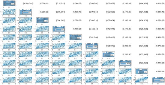
Figure 4.
Estimation results of normalized mixed R-vine copula contour plot, Kendall’s , and Spearman’s for 10 stock indices in the 100-dimensional cases using R-vine–ICAPM–EGARCH–Mixture model and VBDA1 method. Notes: Due to space, only 10 representative stocks are shown. Contour plots are shown in the lower triangular matrix while [Kendall’s , Spearman’s ] are shown in the upper triangular matrix.
Table 1 summarizes the model performance for the 30-dimensional case. Based on the training dataset, the proposed VBDA1–R-vine–ICAPM–EGARCH–mixture model delivers the best performance in terms of marginal likelihood. The next best performers are the VBDA2 and VBDA0 methods, respectively. Among all estimation methods, VBDA2 is the most computationally intensive, which explains its longer runtime for R-vine copula estimation. VBDA1, while still relatively complex, requires less computing time than VBDA2 and converges more efficiently than simpler methods such as VBDA0 due to its favorable convergence properties.
An illustration of the convergence behavior of the evidence lower bound (ELBO) for all VBDA methods is shown in Figure 5, using the stock index pair (DE, CAT) as an example. Additionally, Figure 6 presents the first tree structure from the spanning tree maximization algorithm for the VBDA2–R-vine–ICAPM–EGARCH–mixture model. In contrast, when evaluating by Akaike information criterion (AIC), Bayesian information criterion (BIC), and log-likelihood values, the QMLE–R-vine–ARMA–GARCH–Student-t model achieves the best performance. The second-best performance under these criteria is the rw-MH-based R-vine–ICAPM–EGARCH–mixture model, which achieves a favorable acceptance rate in the MH algorithm.
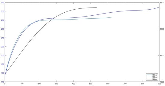
Figure 5.
An example of ELBO convergence across VBDA methods for a pair of stocks (DE, CAT), using a Student-t copula in the 30-dimensional case. Note: The ELBO values of VBDA0 are plotted against the right y-axis while those of VBDA1 and VBDA2 are plotted against the left y-axis.
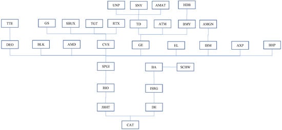
Figure 6.
An example of Tree 1 in the 30-dimensional case of an R-vine copula using VBDA2 within the R-vine–ICAPM–EGARCH–Mixture model.
For the test dataset, forecasting performance was evaluated over one-month and three-month horizons using the MAD and RMSE metrics. In terms of forecast errors, the QMLE and rw-MH methods show comparable predictive performance and emerge as the best-performing models overall. Interestingly, within the variational Bayes framework, VBDA1 demonstrates improved performance—especially as the forecast horizon increases—outperforming the other VBDA variants based on MAD values. This trend is further supported by the experimental results.
Table 2 summarizes the performance of the proposed models in the 100-dimensional setting, using both training and test datasets. Overall, as the number of dimensions increases to 100, the performance of variational Bayes methods improves noticeably.
Among all approaches, the Bayesian inference and machine learning methods—particularly the Variational Bayes with Data Augmentation Type 1 (VBDA1)—outperform the traditional QMLE method, especially in terms of the mean absolute deviation (MAD) for the three-month forecast horizon. The VBDA1–R-vine–ICAPM–EGARCH–mixture model achieves the lowest three-month MAD, accurate to three decimal places, indicating superior forecasting accuracy.
These findings suggest that variational Bayes—specifically, the VBDA1 algorithm—performs effectively in high-dimensional settings. Both the training and test results confirm that the VBDA1–R-vine–ICAPM–EGARCH–mixture model surpasses all competing models in terms of marginal likelihood and three-month MAD forecast error.
Based on the model comparisons, the rw-MH algorithm combined with the R-vine-ICAPM-EGARCH-Mixture model emerges as the most outstanding, particularly due to its reasonable acceptance rate. Variational Bayes inference also performs exceptionally well, with the VBDA0-R-vine-ICAPM-EGARCH-Mixture model ranking as the second most preferable according to the AIC and BIC values. While the traditional QMLE method shows a decline in performance on the training data, it still remains a viable alternative for the test data.
Table 3 and Table 4 summarize the copula families and their parameter counts across models and methods for 30- and 100-dimensional settings, as selected by Algorithm 1. In total, there are 435 pair-copula functions in 30 dimensions and 4950 in 100 dimensions. In the 30-dimensional case, the best-performing method—VBDA1—estimates 638 parameters, which is the second-lowest among all methods. Conversely, in the 100-dimensional case, VBDA1 estimates 6138 parameters—the highest. This indicates that better model performance does not necessarily correspond to a smaller number of parameters. Among the selected bivariate copula families, the elliptical copulas—Student-t and Gaussian—fit the empirical data best, followed by Archimedean families. The Student-t, Gaussian, and Frank copulas together account for at least 68% of all copulas used, implying that approximately 32% of the data exhibit asymmetric or tail dependence characteristics. In 30 dimensions, the most frequently selected families are Student-t and Frank, while in 100 dimensions, the elliptical copulas dominate. Notably, the BB6 copula was not selected in the 30-dimensional case, and the BB10 copula was not used in the 100-dimensional case.
Table 3.
Summary of copula families and their parameter numbers across models and methods for 30 dimensions.
Table 4.
Summary of copula families and their parameter numbers across models and methods for 100 dimensions.
In this study, we apply the ICAPM–EGARCH–mixture with R-vine copula, which we believe is a useful model. However, this might be subject to the model misspecification, which can be a limitation of this study. The computing performance is another possible limitation, which can be improved, but we leave for future research. A practical implementation from the practitioner’s viewpoint poses an interesting challenge to be validated in the future.
5. Concluding Remarks
This study introduces the variational Bayes methods—with and without data augmentation types 1 and 2—for Bayesian inference and machine learning, alongside the rw-MH Bayesian MCMC approach and the competing QMLE method, applied to regular vine copula models in graph theory for n-dimensional data. Standard multivariate copulas often face limitations due to having a single control parameter, a problem that worsens as dimensionality increases. Although C-vine and D-vine copulas offer more flexibility by allowing different bivariate copula choices and tree constructions, they impose restrictions on the tree path structure. To overcome this, we employ the more general R-vine copula, which eliminates the tree path structure constraint and provides richer insights into the relationships within financial data. This study considers 13 candidate bivariate copula families for the R-vine model, though the algorithm easily accommodates additional families. Furthermore, our proposed model is fully compatible with the special subclasses of C-vine and D-vine copulas and can be applied to n-dimensional data analysis.
Furthermore, this study is the first to introduce a mixture distribution into the R-vine model, enhancing its flexibility. The mixture distribution combines a Gaussian distribution with two generalized Pareto distributions within a univariate marginal intertemporal capital asset pricing model and an asymmetric GARCH framework, capturing additional risk premium stylized facts of specific financial securities. Additionally, the study presents a parallel R-vine with margins algorithm for Bayesian inference and machine learning, a bivariate copula selection algorithm within the R-vine framework, and an R-vine with margins data simulation algorithm. Importantly, our proposed algorithm can compute the joint distribution for arbitrary R-vine copulas.
In conclusion, our study produces the R-vine tree path dependence structure, pair-copula types, and parameter estimates in n-dimensions. The univariate marginal model captures individual stock risk premiums and risk-free rates. Our proposed model, particularly the VBDA1–R-vine–ICAPM–EGARCH–mixture model, outperforms competing approaches. Moreover, we demonstrate that the traditional QMLE estimation method significantly deteriorates as dimensionality increases.
For future research, there are numerous avenues to explore depending on specific interests. For instance, the model could be applied to higher-frequency data or extended with alternative copula families such as factor copulas or rotated copulas. The copula selection criteria could also be modified—using Spearman’s or other relevant measures tailored to particular financial contexts instead of Kendall’s . Additionally, the framework can be adapted to other domains, such as high-dimensional portfolio optimization and higher-dimensional datasets. From a computational perspective, further development could involve implementing the algorithm on high-performance computing platforms to reduce computational time in Bayesian inference and machine learning.
Supplementary Materials
The following supporting information can be downloaded at: https://www.mdpi.com/article/10.3390/math13233886/s1.
Author Contributions
Conceptualization, R.K. and N.W.; methodology, R.K.; software, R.K.; validation, R.K. and N.W.; formal analysis, R.K.; data curation, R.K.; writing—original draft preparation, R.K.; writing—review and editing, N.W.; visualization, R.K.; supervision, N.W. All authors have read and agreed to the published version of the manuscript.
Funding
This research received no external funding.
Data Availability Statement
The raw data supporting the conclusions of this article will be made available by the authors on request.
Acknowledgments
We thank the reviewers for their useful comments and feedback that help improve the manuscript.
Conflicts of Interest
The authors declare no conflicts of interest.
Appendix A. Some Parametric Copula Families and Their Properties
This appendix presents the dependence structure of all copula families used in this study including one- and two-parameter copulas. The elliptical copulas are the Gaussian (normal) copula and Student-t copula. The bivariate copula distributions of Gaussian and Student-t, respectively, are
where is an inverse cumulative Gaussian distribution function. is a correlation matrix; is a continuous standard uniform random variable; is an inverse cumulative Student-t distribution function; is the cdf of bivariate distribution where degree of freedom. The copula is denoted as . It is worth mentioning that where is a bivariate survival function and are monotonically decreasing transforms. Therefore, the conditional cdf and copula pdf are:
The bivariate cdf copula families in this study including one and two parameters are presented in Table A1 while their tail dependence measures are shown in Table A2.
Table A1.
Some parametric copula distributions.
Table A1.
Some parametric copula distributions.
| Copula | Bivariate Function | Parameter |
|---|---|---|
| One-parameter | ||
| Gumbel | ||
| Clayton | ||
| Frank | ||
| Joe/B5 | ||
| Galambos | ||
| Two-parameters | ||
| BB1 | ||
| BB3 | ||
| BB4 | ||
| BB5 | ||
| BB7 | ||
| BB10 | ||
Table A2.
Tail dependence measures of some parametric copulas.
Table A2.
Tail dependence measures of some parametric copulas.
| Copula | or | or |
|---|---|---|
| One-parameter | ||
| Gaussian/Normal | ||
| Gumbel (extreme value) | ||
| Clayton | ||
| Frank | ||
| Joe/B5 | ||
| Galambos (extreme value) | ||
| Two-parameters | ||
| Student-t | ||
| BB1 | ||
| BB3 | ||
| BB4 | ||
| BB5 (extreme value) | ||
| BB7 | ||
| BB10 |
A rank-based measurement of the dependence measure of the copula families can be computed either from a closed-form solution (if available) or numerical approximation via a Monte Carlo simulation through two-variable integrals as in Equation (A1) for Kendall’s and Equation (A2) for Spearman , respectively.
Note that a closed-form Kendall’s and Spearman of Gaussian copula, t copula, Gumbel copula, Frank copula, and Clayton copula are used. Otherwise, we use Monte Carlo approximation.
Appendix B. Independence Test Results of the Standardized Residuals
This appendix discusses the Ljung–Box independence testing of the marginal model residuals of this study including ICAPM-EGARCH with mixture innovation and the competing ARMA-GARCH with Student-t innovation with the estimation method of rw-MH, variational Bayes and QMLE. For the 100 stocks, standardized residuals of all the proposed models indicated independence where meant failure to reject the null hypothesis that the residuals are independently distributed, except for the stock abbreviations ‘V’, ‘MA’, ‘TXN’, ‘QCOM’, ‘SCHW’ and ‘DEO’ in ICAPM-EGARCH(1,1)-Mixture-rw-MH model. For the ICAPM-EGARCH(1,1)-Mixture-VBDA0 model, the stock abbreviations are ‘V’, ‘TXN’, ‘QCOM’ and ‘DEO’. For the ICAPM-EGARCH(1,1)-Mixture-VBDA1 model, the stock abbreviations are ‘V’, ‘MA’, ‘TXN’, ‘QCOM’ and ‘DEO’. For ICAPM-EGARCH(1,1)-Mixture-VBDA2 model, the stock abbreviations are ‘V’, ‘TXN’, ‘QCOM’ and ‘DEO’. For ICAPM-EGARCH(1,1)-Mixture-QMLE model, the stock abbreviations are ‘V’, ‘MA’, ‘TXN’, ‘QCOM’, ‘SCHW’ and ‘DEO’. For ARMA(1,1)-GARCH(1,1)-t-QMLE model, the stock abbreviations are ‘QCOM’and ‘HON’.
Appendix C. List of 100 Nasdaq Stocks Used in the Study (The Last 30 Stocks Used in the 30-Dimensional Analysis)
| No | Symbol | Name | Sector |
| 1 | AAPL | Apple Inc. Common Stock | Technology |
| 2 | MSFT | Microsoft Corporation Common Stock | Technology |
| 3 | GOOG | Alphabet Inc. Class C Capital Stock | Technology |
| 4 | GOOGL | Alphabet Inc. Class A Common Stock | Technology |
| 5 | AMZN | Amazon.com Inc. Common Stock | Consumer Services |
| 6 | MCHP | Microchip Technology Incorporated Common Stock | Technology |
| 7 | TSM | Taiwan Semiconductor Manufacturing Company Ltd. | Technology |
| 8 | NVDA | NVIDIA Corporation Common Stock | Technology |
| 9 | V | Visa Inc. | Miscellaneous |
| 10 | JPM | JP Morgan Chase & Co. Common Stock | Finance |
| 11 | IDXX | IDEXX Laboratories Inc. Common Stock | Health Care |
| 12 | JNJ | Johnson & Johnson Common Stock | Health Care |
| 13 | WMT | Walmart Inc. Common Stock | Consumer Services |
| 14 | UNH | United Health Group Incorporated Common Stock (DE) | Health Care |
| 15 | ADI | Analog Devices Inc. Common Stock | Technology |
| 16 | HD | Home Depot Inc. (The) Common Stock | Consumer Services |
| 17 | ASML | ASML Holding N.V. New York Registry Shares | Technology |
| 18 | PG | Procter & Gamble Company (The) Common Stock | Consumer Non-Durables |
| 19 | BAC | Bank of America Corporation Common Stock | Finance |
| 20 | MA | Mastercard Incorporated Common Stock | Miscellaneous |
| 21 | KLAC | KLA Corporation Common Stock | Capital Goods |
| 22 | DIS | Walt Disney Company (The) Common Stock | Consumer Services |
| 23 | ADBE | Adobe Inc. Common Stock | Technology |
| 24 | CMCSA | Comcast Corporation Class A Common Stock | Consumer Services |
| 25 | NFLX | Netflix Inc. Common Stock | Consumer Services |
| 26 | CRM | Salesforce.com Inc Common Stock | Technology |
| 27 | PFE | Pfizer Inc. Common Stock | Health Care |
| 28 | TM | Toyota Motor Corporation Common Stock | Capital Goods |
| 29 | NKE | Nike Inc. Common Stock | Consumer Non-Durables |
| 30 | CSCO | Cisco Systems Inc. Common Stock (DE) | Technology |
| 31 | ORCL | Oracle Corporation Common Stock | Technology |
| 32 | KO | Coca-Cola Company (The) Common Stock | Consumer Non-Durables |
| 33 | TMO | Thermo Fisher Scientific Inc Common Stock | Capital Goods |
| 34 | DHR | Danaher Corporation Common Stock | Health Care |
| 35 | NVO | Novo Nordisk A/S Common Stock | Health Care |
| 36 | XOM | Exxon Mobil Corporation Common Stock | Energy |
| 37 | VZ | Verizon Communications Inc. Common Stock | Public Utilities |
| 38 | LLY | Eli Lilly and Company Common Stock | Health Care |
| 39 | ABT | Abbott Laboratories Common Stock | Health Care |
| 40 | INTC | Intel Corporation Common Stock | Technology |
| 41 | NTES | NetEase Inc. American Depositary Shares | Miscellaneous |
| 42 | PEP | PepsiCo Inc. Common Stock | Consumer Non-Durables |
| 43 | ACN | Accenture plc Class A Ordinary Shares (Ireland) | Technology |
| 44 | COST | Costco Wholesale Corporation Common Stock | Consumer Services |
| 45 | T | AT&T Inc. | Consumer Services |
| 46 | WFC | Wells Fargo & Company Common Stock | Finance |
| 47 | NVS | Novartis AG Common Stock | Health Care |
| 48 | CVX | Chevron Corporation Common Stock | Energy |
| 49 | MRK | Merck & Company Inc. Common Stock (new) | Health Care |
| 50 | AZN | AstraZeneca PLC American Depositary Shares | Health Care |
| 51 | MS | Morgan Stanley Common Stock | Finance |
| 52 | MCD | McDonald’s Corporation Common Stock | Consumer Services |
| 53 | TXN | Texas Instruments Incorporated Common Stock | Technology |
| 54 | MDT | Medtronic plc. Ordinary Shares | Health Care |
| 55 | UPS | United Parcel Service Inc. Common Stock | Transportation |
| 56 | SAP | SAP SE ADS | Technology |
| 57 | NEE | NextEra Energy Inc. Common Stock | Public Utilities |
| 58 | PM | Philip Morris International Inc Common Stock | Consumer Non-Durables |
| 59 | TMUS | T-Mobile US Inc. Common Stock | Public Utilities |
| 60 | LIN | Linde plc Ordinary Share | Basic Industries |
| 61 | INTU | Intuit Inc. Common Stock | Technology |
| 62 | QCOM | QUALCOMM Incorporated Common Stock | Technology |
| 63 | HON | Honeywell International Inc. Common Stock | |
| 64 | LOW | Lowe’s Companies Inc. Common Stock | Consumer Services |
| 65 | UL | Unilever PLC Common Stock | Consumer Non-Durables |
| 66 | RY | Royal Bank Of Canada Common Stock | |
| 67 | ILMN | Illumina Inc. Common Stock | Health Care |
| 68 | BHP | BHP Group Limited American Depositary Shares (Each representing two Ordinary Shares) | Basic Industries |
| 69 | C | Citigroup Inc. Common Stock | Finance |
| 70 | SONY | Sony Group Corporation American Depositary Shares | Consumer Non-Durables |
| 71 | HDB | HDFC Bank Limited Common Stock | Finance |
| 72 | BMY | Bristol-Myers Squibb Company Common Stock | Health Care |
| 73 | AMT | American Tower Corporation (REIT) Common Stock | Finance |
| 74 | SBUX | Starbucks Corporation Common Stock | |
| 75 | BLK | BlackRock Inc. Common Stock | Finance |
| 76 | SCHW | Charles Schwab Corporation (The) Common Stock | Finance |
| 77 | UNP | Union Pacific Corporation Common Stock | Transportation |
| 78 | BBL | BHP Group PlcSponsored ADR | Energy |
| 79 | AXP | American Express Company Common Stock | Finance |
| 80 | GS | Goldman Sachs Group Inc. (The) Common Stock | Finance |
| 81 | RTX | Raytheon Technologies Corporation Common Stock | Capital Goods |
| 82 | AMD | Advanced Micro Devices Inc. Common Stock | Technology |
| 83 | BA | Boeing Company (The) Common Stock | Capital Goods |
| 84 | AMAT | Applied Materials Inc. Common Stock | Capital Goods |
| 85 | AMGN | Amgen Inc. Common Stock | Health Care |
| 86 | ISRG | Intuitive Surgical Inc. Common Stock | Health Care |
| 87 | IBM | International Business Machines Corporation Common Stock | Technology |
| 88 | SNY | Sanofi ADS | Health Care |
| 89 | TGT | Target Corporation Common Stock | Consumer Services |
| 90 | TD | Toronto Dominion Bank (The) Common Stock | |
| 91 | TTE | TotalEnergies SE | Energy |
| 92 | EL | Estee Lauder Companies Inc. (The) Common Stock | Consumer Non-Durables |
| 93 | CVS | CVS Health Corporation Common Stock | Health Care |
| 94 | GE | General Electric Company Common Stock | Consumer Durables |
| 95 | DEO | Diageo plc Common Stock | Consumer Non-Durables |
| 96 | SPGI | S&P Global Inc. Common Stock | Technology |
| 97 | RIO | Rio Tinto Plc Common Stock | Basic Industries |
| 98 | JBHT | J.B. Hunt Transport Services Inc. Common Stock | Transportation |
| 99 | DE | Deere & Company Common Stock | Capital Goods |
| 100 | CAT | Caterpillar Inc. Common Stock | Capital Goods |
References
- Sklar, M. Fonctions de repartition an dimensions et leurs marges. Publ. L’Institut Stat. L’Universit’E Paris 1959, 8, 229–231. [Google Scholar]
- Achite, M.; Bazrafshan, O.; Pakdaman, Z.; Simsek, O.; Caloiero, T. Multivariate uncertainty analysis of severity-duration-magnitude frequency curves using Khoudraji copula and bootstrap method. Hydrol. Sci. J. 2025. [Google Scholar] [CrossRef]
- Deng, T.; Zeng, Z.; Xu, J. A copula-based statistical method of estimating production profile from temperature measurement for perforated horizontal wells. Pet. Sci. Technol. 2024, 42, 4589–4609. [Google Scholar] [CrossRef]
- Zhou, C.; van Nooijen, R.; Kolechkina, A.; Gargouri, E.; Slama, F.; van de Giesen, N. The uncertainty associated with the use of copulas in multivariate analysis. Hydrol. Sci. J. 2023, 68, 2169–2188. [Google Scholar] [CrossRef]
- Aghatise, O.; Khan, F.; Ahmed, S. Reliability assessment of marine structures considering multidimensional dependency of the variables. Ocean. Eng. 2021, 230, 109021. [Google Scholar] [CrossRef]
- Chen, P.; Zhang, J. Copula-based multivariate control charts for monitoring multiple dependent Weibull processes. Commun. Stat.-Simul. Comput. 2025, 0, 1–22. [Google Scholar] [CrossRef]
- Farkas, S.; Lopez, O. Semiparametric copula models applied to the decomposition of claim amounts. Scand. Actuar. J. 2024, 2024, 1065–1092. [Google Scholar] [CrossRef]
- Wang, Q.; Wu, X. A Nonparametric Bayesian Estimator of Copula Density with Applications to Financial Market. J. Bus. Econ. Stat. 2025, 43, 1021–1033. [Google Scholar] [CrossRef]
- Kim, J.M.; Ha, I.D.; Kim, S. Copula deep learning control chart for multivariate zero inflated count response variables. Statistics 2024, 58, 749–769. [Google Scholar] [CrossRef]
- McNeil, A.J.; Frey, R.; Embrechts, P. Quantitative Risk Management: Concepts, Techniques and Tools; Princeton Series in Finance; Princeton University Press: Princeton, NJ, USA, 2015. [Google Scholar]
- Wichitaksorn, N.; Gerlach, R.; Choy, S.T.B. Efficient MCMC estimation of some elliptical copula regression models through scale mixtures of normals. Appl. Stoch. Model. Bus. Ind. 2019, 35, 808–822. [Google Scholar] [CrossRef]
- Górecki, J.; Hofert, M.; Okhrin, O. Outer power transformations of hierarchical Archimedean copulas: Construction, sampling and estimation. Comput. Stat. Data Anal. 2021, 155, 107109. [Google Scholar] [CrossRef]
- Liang, P.; Rosen, O. Flexible Bayesian estimation of elliptical copulas. J. Comput. Graph. Stat. 2025, 0, 1–18. [Google Scholar] [CrossRef]
- Michaelides, M.; Cossette, H.; Pigeon, M. Simulations of Bivariate Archimedean Copulas from Their Nonparametric Generators for Loss Reserving under Flexible Censoring. N. Am. Actuar. J. 2025, 0, 1–28. [Google Scholar] [CrossRef]
- Aas, K.; Czado, C.; Frigessi, A.; Bakken, H. Pair-copula constructions of multiples dependence. Insur. Math. Econ. 2009, 44, 182–198. [Google Scholar] [CrossRef]
- Kurowicka, D.; Cooke, R.M. Distribution-free continuous Bayesian belief nets. In Modern Statistical and Mathematical Methods in Reliability; World Scientific: Singapore, 2005; Volume 10, pp. 309–322. [Google Scholar]
- Joe, H. Dependence Modelling with Copulas; Monographs on Statistics and Applied Probability: 134; CRC Press: Boca Raton, FL, USA, 2015. [Google Scholar]
- Müller, D.; Czado, C. Representing sparse Gaussian DAGs as sparse R-vines Allowing for Non-Gaussian Dependence. J. Comput. Graph. Stat. 2018, 27, 334–344. [Google Scholar] [CrossRef]
- Müller, D.; Czado, C. Dependence modelling in ultra high dimensions with vine copulas and the Graphical Lasso. Comput. Stat. Data Anal. 2019, 137, 211–232. [Google Scholar] [CrossRef]
- Brechmann, E.C.; Czado, C.; Aas, K. Truncated regular vines in high dimensions with application to financial data. Can. J. Stat. 2012, 40, 68–85. [Google Scholar] [CrossRef]
- Maya, R.A.L.; Gomez-Gonzalez, J.E.; Velandia, L.F.M. Latin American exchange rate dependencies: A regular vine copula approach. Contemp. Econ. Policy 2015, 33, 535–549. [Google Scholar] [CrossRef]
- Li, H.; Liu, Z.; Wang, S. Vines climbing higher: Risk management for commodity futures markets using a regular vine copula approach. Int. J. Financ. Econ. 2022, 27, 2438–2457. [Google Scholar] [CrossRef]
- Xiao, Q.; Yan, M.; Zhang, D. Commodity market financialization, herding and signals: An asymmetric GARCH R-vine copula approach. Int. Rev. Financ. Anal. 2023, 89, 102743. [Google Scholar] [CrossRef]
- Čeryová, B.; Árendáš, P. Vine copula approach to the intra-sectoral dependence analysis in the technology industry. Financ. Res. Lett. 2024, 60, 104889. [Google Scholar] [CrossRef]
- Hamza, T.; Ben Haj Hamida, H.; Mili, M.; Sami, M. High inflation during Russia–Ukraine war and financial market interaction: Evidence from C-Vine Copula and SETAR models. Res. Int. Bus. Financ. 2024, 70, 102384. [Google Scholar] [CrossRef]
- Czado, C. Pair-Copula Constructions of Multivariate Copulas. In Copula Theory and Its Applications; Jaworski, P., Durante, F., Härdle, W.K., Rychlik, T., Eds.; Springer: Berlin/Heidelberg, Germany, 2010; pp. 93–109. [Google Scholar]
- Joe, H.; Li, H.; Nikoloulopoulos, A.K. Tail dependence functions and vine copulas. J. Multivar. Anal. 2010, 101, 252–270. [Google Scholar] [CrossRef]
- Patton, A.J. A review of copula models for economic time series. J. Multivar. Anal. 2012, 110, 4–18. [Google Scholar] [CrossRef]
- Fan, Y.; Patton, A.J. Copulas in econometrics. Annu. Rev. Econ. 2014, 6, 179–200. [Google Scholar] [CrossRef]
- Dißmann, J.; Brechmann, E.C.; Czado, C.; Kurowicka, D. Selecting and estimating regular vine copulae and application to financial returns. Comput. Stat. Data Anal. 2013, 59, 52–69. [Google Scholar] [CrossRef]
- Vuong, Q.H. Likelihood ratio tests for model selection and non-nested Hypotheses. Econometrica 1989, 57, 307–333. [Google Scholar] [CrossRef]
- Merton, R.C. An intertemporal capital asset pricing model. Econometrica 1973, 41, 867–887. [Google Scholar] [CrossRef]
- Sun, F.; Fu, F.; Liao, H.; Xu, D. Analysis of multivariate dependent accelerated degradation data using a random-effect general Wiener process and D-vine Copula. Reliab. Eng. Syst. Saf. 2020, 204, 107168. [Google Scholar] [CrossRef]
- Nagler, T.; Bumann, C.; Czado, C. Model selection in sparse high-dimensional vine copula models with an application to portfolio risk. J. Multivar. Anal. 2019, 172, 180–192. [Google Scholar] [CrossRef]
- Chang, B.; Joe, H. Prediction based on conditional distributions of vine copulas. Comput. Stat. Data Anal. 2019, 139, 45–63. [Google Scholar] [CrossRef]
- Mantel, N.; Myers, M. Problems of convergence of maximum likelihood iterative procedures in multiparameter situations. J. Am. Stat. Assoc. 1971, 66, 484–491. [Google Scholar] [CrossRef]
- Loaiza-Maya, R.; Smith, M.S. Variational Bayes estimation of discrete-margined copula models with application to time series. J. Comput. Graph. Stat. 2019, 28, 523–539. [Google Scholar] [CrossRef]
- Chang, C.L.; McAleer, M.; Wong, W.K. Big data, computational science, economics, finance, marketing, management, and psychology: Connections. J. Risk Financ. Manag. 2018, 11, 15. [Google Scholar] [CrossRef]
- Oh, D.H.; Patton, A.J. High-dimensional copula-based distributions with mixed frequency data. J. Econom. 2016, 193, 349–366. [Google Scholar] [CrossRef]
- Pareek, M.K.; Thakkar, P. Surveying stock market portfolio optimization techniques. In Proceedings of the 2015 5th Nirma University International Conference on Engineering (NUiCONE), Ahmedabad, India, 26–28 November 2015; pp. 1–5. [Google Scholar]
- Kolm, P.N.; Tütüncü, R.; Fabozzi, F.J. 60 Years of portfolio optimization: Practical challenges and current trends. Eur. J. Oper. Res. 2014, 234, 356–371. [Google Scholar] [CrossRef]
- Bedford, T.; Cooke, R.M. Probability density decomposition for conditionally dependent random variables modeled by vines. Ann. Math. Artif. Intell. 2001, 32, 245–268. [Google Scholar] [CrossRef]
- Bedford, T.; Cooke, R.M. Vines: A new graphical model for dependent random variables. Ann. Stat. 2002, 30, 1031–1068. [Google Scholar] [CrossRef]
- Kurowicka, D.; Joe, H. (Eds.) Dependence Modeling: Vine Copula Handbook; World Scientific: Singapore, 2010. [Google Scholar]
- Hafner, C.M.; Kyriakopoulou, D. Exponential-Type GARCH models with linear-in-variance risk premium. J. Bus. Econ. Stat. 2021, 39, 589–603. [Google Scholar] [CrossRef]
- Nelson, D.B. Conditional heteroskedasticity in asset returns: A new approach. Econometrica 1991, 59, 347–370. [Google Scholar] [CrossRef]
- Hentschel, L. All in the family nesting symmetric and asymmetric GARCH models. J. Financ. Econ. 1995, 39, 71–104. [Google Scholar] [CrossRef]
- Jose Rodriguez, M.; Ruiz, E. Revisiting several popular GARCH models with leverage effect: Differences and similarities. J. Financ. Econom. 2012, 10, 637–668. [Google Scholar] [CrossRef]
- Sahamkhadam, M.; Stephan, A.; Östermark, R. Portfolio optimization based on GARCH-EVT-Copula forecasting models. Int. J. Forecast. 2018, 34, 497–506. [Google Scholar] [CrossRef]
- Engle, R. Risk and volatility: Econometric models and financial practice. Am. Econ. Rev. 2004, 94, 405–420. [Google Scholar] [CrossRef]
- Hosking, J.R.M.; Wallis, J.R. Parameter and Quantile Estimation for the generalized Pareto Distribution. Technometrics 1987, 29, 339–349. [Google Scholar] [CrossRef]
- Singh, V.P.; Guo, H. Parameter estimation for 3-parameter generalized Pareto distribution by the principle of maximum entropy (POME). Hydrol. Sci. J. 1995, 40, 165–181. [Google Scholar] [CrossRef]
- Koop, G.; Poirier, D.J.; Tobias, J.L. Bayesian Econometric Methods; Econometric Exercises; Cambridge University Press: Cambridge, UK, 2007. [Google Scholar]
- Scherr, S.; Zhou, J. Automatically Identifying Relevant Variables for Linear Regression with the Lasso Method: A Methodological Primer for its Application with R and a Performance Contrast Simulation with Alternative Selection Strategies. Commun. Methods Meas. 2020, 14, 204–211. [Google Scholar] [CrossRef]
- Nezamdoust, S.; Eskandari, F. Ridge Shrinkage Estimators in Finite Mixture of Generalized Estimating Equations. J. Math. Model. Financ. 2022, 2, 91–106. [Google Scholar]
- Liang, C.; Xu, Y.; Chen, Z.; Li, X. Forecasting China’s stock market volatility with shrinkage method: Can Adaptive Lasso select stronger predictors from numerous predictors? Int. J. Financ. Econ. 2022, 28, 3689–3699. [Google Scholar] [CrossRef]
- Al Janabi, M.A.M.; Arreola Hernandez, J.; Berger, T.; Nguyen, D.K. Multivariate dependence and portfolio optimization algorithms under illiquid market scenarios. Eur. J. Oper. Res. 2017, 259, 1121–1131. [Google Scholar] [CrossRef]
- Yu, W.; Bondell, H.D. Variational Bayes for Fast and Accurate Empirical Likelihood Inference. J. Am. Stat. Assoc. 2024, 119, 1089–1101. [Google Scholar] [CrossRef]
- Gunawan, D.; Tran, M.N.; Suzuki, K.; Dick, J.; Kohn, R. Computationally efficient Bayesian estimation of high-dimensional Archimedean copulas with discrete and mixed margins. Stat. Comput. 2019, 29, 933–946. [Google Scholar] [CrossRef]
- Tran, M.N.; Nguyen, T.N.; Dao, V.H. A practical tutorial on variational Bayes. arXiv 2021, arXiv:2103.01327. [Google Scholar] [CrossRef]
- Blei, D.M.; Kucukelbir, A.; McAuliffe, J.D. Variational inference: A review for statisticians. J. Am. Stat. Assoc. 2017, 112, 859–877. [Google Scholar] [CrossRef]
- Smith, M.S.; Loaiza-Maya, R.; Nott, D.J. High-dimensional copula variational approximation through transformation. J. Comput. Graph. Stat. 2020, 29, 729–743. [Google Scholar] [CrossRef]
- Ong, V.M.H.; Nott, D.J.; Smith, M.S. Gaussian variational approximation with a factor covariance structure. J. Comput. Graph. Stat. 2018, 27, 465–478. [Google Scholar] [CrossRef]
- Zeiler, M.D. ADADELTA: An Adaptive Learning Rate Method. arXiv 2012, arXiv:1212.5701. [Google Scholar] [CrossRef]
- Morales Napoles, O.; Cooke, R.M.; Kurowicka, D. About the Number of Vines and Regular Vines on n Nodes (Submitted for Publication). 2010. Available online: https://resolver.tudelft.nl/uuid:912abf55-8112-48d2-9cca-323f7f6aecc7 (accessed on 17 November 2025).
- Nikoloulopoulos, A.K.; Joe, H.; Li, H. Vine copulas with asymmetric tail dependence and applications to financial return data. Comput. Stat. Data Anal. 2012, 56, 3659–3673. [Google Scholar] [CrossRef]
Disclaimer/Publisher’s Note: The statements, opinions and data contained in all publications are solely those of the individual author(s) and contributor(s) and not of MDPI and/or the editor(s). MDPI and/or the editor(s) disclaim responsibility for any injury to people or property resulting from any ideas, methods, instructions or products referred to in the content. |
© 2025 by the authors. Licensee MDPI, Basel, Switzerland. This article is an open access article distributed under the terms and conditions of the Creative Commons Attribution (CC BY) license (https://creativecommons.org/licenses/by/4.0/).