Robustness of Identifying Item–Trait Relationships Under Non-Normality in MIRT Models

Abstract

Identifying item–trait relationships is a core task in multidimensional item response theory (MIRT). Common empirical approaches include exploratory item factor analysis (EIFA) with rotations, the expectation maximization-based $L_1$ regularization (EML1) algorithm, and the expectation model selection (EMS) algorithm. While these methods typically assume multivariate normality of latent traits, empirical data often deviate from this assumption. This study evaluates the robustness of EIFA, EML1, and EMS, when latent traits violate normality assumptions. Using the independent generator transform, we generate latent variables under varying levels of skewness, excess kurtosis, numbers of non-normal dimensions, and inter-factor correlations. We then assess the performance of each method in terms of the F1-score for identifying item–trait relationships and mean squared error (MSE) of parameter estimations. The results indicate that non-normality leads to a reduction in F1-score and an increase in MSE generally. For F1-score, EMS performs best with small samples (e.g., $N=500$), whereas EIFA with rotations yields the highest F1-score in larger samples. In terms of estimation accuracy, EMS and EML1 generally yield lower MSEs than EIFA. The effects of non-normality are also demonstrated by applying these methods to a real data set from the Depression, Anxiety, and Stress Scale.

1. Introduction

In psychological and educational testing, dichotomous and polytomous items are widely used to assess individuals’ latent traits or abilities. When multiple latent dimensions are involved, a central task is to identify the underlying relationships between items and latent traits. Traditionally, such relationships are determined a priori by domain experts based on their knowledge of item content and construct definitions. However, the correct specification of item–trait associations is critical, not only for accurate model calibration but also for valid individual assessment. Misclassification of these associations can result in serious model misfit and flawed diagnostic interpretations. Therefore, an important question is to empirically estimate the underlying item–trait relationships from the data. In this paper, we consider this question within the framework of MIRT models.

More specifically, each subject is characterized by a random latent trait vector $\mathit{\theta }={({\theta }_1,\dots ,{\theta }_K)}^{\top }$ in a MIRT model. The probability of a correct response to item j is modeled as $P(Y_j=1\mid \mathit{\theta })=F({\mathit{a}}_j^{\top }\mathit{\theta }+b_j),$ where ${\mathit{a}}_j={(a_{j1},\dots ,a_{jK})}^{\top }$ and $b_j$ are the discrimination and difficulty parameters, respectively. Essentially, the detection of item–trait relationships corresponds to the identification of the nonzero elements of ${\mathit{a}}_j$.

There are three primary approaches for empirically estimating the underlying relationships between items and latent traits. A commonly used approach is exploratory item factor analysis (EIFA). It estimates all parameters (under location and scale constraints on the latent traits), applies an analytic rotation, and then imposes a cutoff on the rotated discrimination matrix to obtain a simpler, interpretable structure with some zero elements [1,2,3]. As an alternative, $L_1$ regularized methods are proposed [4,5,6]. These methods impose an $L_1$ penalty on the log-likelihood, shrinking small discrimination parameters toward zero. The performance of $L_1$-regularized methods depends critically on the choice of regularization parameters, which are typically selected by minimizing the Bayesian Information Criterion (BIC; [7]). To avoid the selection of regularization parameters, Xu et al. [8] develops the expectation model selection (EMS) and Shang et al. [9] proposes generalized EMS algorithms. Both algorithms directly minimize BIC to explore item–trait relationships. Further methodological details are provided in Section 2.

It should be noted that most of preceding methods assume that latent traits $\mathit{\theta }$ in Equation (1) follow a multivariate normal distribution. Empirical evidence, however, shows that this assumption is often unrealistic. In clinical assessments, many respondents report no symptoms, creating strong floor effects and non-normal latent traits [10]. Likewise, in psychiatric research, latent variables reflecting psychological disorders are typically positively skewed, as most individuals show low pathology and only a few show severe levels [11]. Similarly, psychological constructs such as depression, pain, and gambling often display non-normal distribution characteristics in the general population [12]. Even when the population distribution is normal, non-random sampling techniques can induce non-normality in the sampled latent traits [13]. For example, when analyzing test scores solely from honors program students, one may obtain a negatively skewed ability distribution.

Many studies investigate the impact of non-normal latent traits on parameter estimation in item response theory (IRT) models. Stone [14] reports that estimation bias increases as latent traits deviate from normality. Finch and Edwards [15] further demonstrates that severe skewness can still distort discrimination parameters even when the sample size is large. Related findings appear in MIRT models. Svetina et al. [16] shows that skewed latent traits reduce the accuracy of discrimination estimates, particularly under complex loading structures and higher inter-factor correlations. Wang et al. [17] extends this investigation to polytomous data under the multidimensional graded response model (MGRM), showing that full-information maximum likelihood reduces bias more effectively than weighted least squares. More recently, McClure and Jacobucci [18] evaluates the Metropolis–Hastings Robbins–Monro algorithm in high-dimensional MGRM models and observes increasing discrimination bias as dimensionality and factor correlations rise. Collectively, these studies underscore that violations of normality substantially reduce parameter recovery accuracy.

While confirmatory item factor analysis under non-normality is widely studied, the robustness of methods for identifying item–trait relationships remains underexplored. This study evaluates the performance of EIFA with rotations, the $L_1$-regularized method, and the EMS algorithm in recovering item–trait structures when latent traits deviate from normality. To conduct this investigation, a method for generating latent variables with controlled deviations from normality is required. A commonly used technique is the Vale–Maurelli (VM) transformation [19], which allows specification of skewness, kurtosis, and a target correlation matrix. However, prior studies show that the VM method often produces biased or unstable estimates of skewness and kurtosis [20], and its dependence structure is closely related to the multivariate normal copula [21]. To generate stronger forms of multivariate non-normality, Foldnes and Olsson [22] proposes the independent generator (IG) transform, which creates non-normal data through linear combinations of independent generator variables. The resulting distributions have a genuinely non-normal copula, and empirical studies indicate that the IG transform produces more pronounced departures from normality than the VM method [22]. Thus, this study employs the IG transform to simulate latent variables under varying levels of skewness, excess kurtosis, numbers of non-normal latent dimensions, and inter-factor correlations, following Svetina et al. [16], Wang et al. [17], and McClure and Jacobucci [18]. We then evaluate each method’s performance using the F1-score for recovering item–trait relationships and the mean squared error (MSE) for parameter estimation. These results provide practical guidance for identifying the item–trait relationships under non-normal latent distributions.

The rest of the article is organized as follows. In Section 2, we first review three methods (EIFA with rotations, EML1, and EMS) within the multidimensional 2-parameter logistic (M2PL) model framework. In Section 3, we describe the IG transform and generate two types of non-normal latent trait distributions. We then conduct two simulations to compare the robustness of the methods for identifying item–trait relationships under non-normality in Section 4. In Section 5, we analyze a real data set. Finally, we summarize the key findings and outline directions for future research.

2. Methods for Identifying the Item–Trait Relationships in the M2PL Model

2.1. The M2PL Model

We focus on the M2PL model, one of the most widely used MIRT models. For subject $i=1,\dots ,N$ and item $j=1,\dots ,J$, let $y_{ij}$ be the binary response from subject i to item j and $Y={\left(y_{ij}\right)}_{N\times J}$ be the response matrix. The item response function for subject i on item j is given by

$$F({\mathit{a}}_j^{\top }{\mathit{\theta }}_i+b_j)={\displaystyle \frac{\exp ({\mathit{a}}_j^{\top }{\mathit{\theta }}_i+b_j)}{1+\exp ({\mathit{a}}_j^{\top }{\mathit{\theta }}_i+b_j)}}.$$

(1)

The latent traits ${\mathit{\theta }}_i$, for $i=1,\dots ,N$, are assumed to be independent and identically distributed, following a K-dimensional normal distribution $N(\mathbf{0},\mathsf{\Sigma })$, where $\mathsf{\Sigma }={\left({\sigma }_{k{k}^{\prime }}\right)}_{K\times K}$ is the covariance matrix with unit variances. Conditional on ${\mathit{\theta }}_i$, item responses are locally independent. Under these assumptions, the marginal log-likelihood is

$$\ell (\mathit{A},\mathit{b},\mathsf{\Sigma }\mid \mathit{Y})=\sum _{i=1}^N\log \left[{\int }_{{\mathit{\theta }}_i\in {\mathcal{R}}^K}\phi ({\mathit{\theta }}_i\mid \mathsf{\Sigma })\prod _{j=1}^{J}F{({\mathit{a}}_j^{\top }{\mathit{\theta }}_i+b_j)}^{y_{ij}}{\left[1-F({\mathit{a}}_j^{\top }{\mathit{\theta }}_i+b_j)\right]}^{1-y_{ij}}\mathrm{d}{\mathit{\theta }}_i\right],$$

(2)

where $\phi ({\mathit{\theta }}_i\mid \mathsf{\Sigma })$ is the density of $N(\mathbf{0},\mathsf{\Sigma })$.

2.2. Exploratory Item Factor Analysis with Rotations

EIFA estimates the discrimination parameters $\mathit{A}$ and difficulties $\mathit{b}$ by maximizing the log-likelihood function (2) under the assumption that $\mathsf{\Sigma }$ is the identity matrix. A rotation matrix $\mathit{T}$ is then applied to obtain a simpler structure, yielding a rotated discrimination matrix $\mathsf{\Lambda }=\mathit{A}\mathit{T}$ with some elements close to zero. There are two broad classes of rotation in EIFA: orthogonal and oblique. Orthogonal rotations assume that the latent traits remain uncorrelated, while oblique rotations allow for correlations among traits. In this study, we apply oblique rotations, including Quartimin [23], Geomin [24], and Infomax [3]. Each employs distinct criteria to achieve a simple and interpretable factor structure while accommodating inter-trait correlations. To facilitate interpretation, small discrimination parameters are often thresholded to zero.

2.3. Expectation Maximization-Based $L_1$ Regularization Method

In MIRT models, identifying the item–trait relationship structure can be framed as a model selection problem with missing data. Specifically, the dependence of item responses on latent traits follows the framework of a generalized linear model, where the latent traits ${\mathit{\theta }}_i$ serve as unobserved covariates and the discrimination parameters ${\mathit{a}}_j$ act as regression coefficients. Identifying the nonzero entries in ${\mathit{a}}_j$ reveals the item’s associated traits. This forms a latent variable selection problem [4]. Each possible zero-nonzero configuration of the discrimination matrix $\mathit{A}$ defines a distinct candidate MIRT model, as it specifies a unique pattern of item–trait associations across all items. Selecting the optimal item–trait structure is thus equivalent to choosing the best model among $2^{JK}$ candidate models. This is fundamentally a model selection problem with missing covariates. Exhaustively evaluating all candidate models is computationally infeasible, even for moderately sized assessments. To address this challenge, the $L_1$-regularized methods [4,5,6] are proposed.

The $L_1$-penalized estimator is defined as

$$({\widehat{\mathit{A}}}_{\eta },{\widehat{\mathit{b}}}_{\eta },{\widehat{\mathsf{\Sigma }}}_{\eta })=\underset{\mathit{A},\mathit{b},\mathsf{\Sigma }}{\arg \max }l(\mathit{A},\mathit{b},\mathsf{\Sigma }\mid \mathit{Y})-\eta {\parallel \mathit{A}\parallel }_1,$$

(3)

where ${\parallel \mathit{A}\parallel }_1={\sum }_{j=1}^J{\sum }_{k=1}^K\left|a_{jk}\right|$ denotes the entry-wise $L_1$ norm of the matrix $\mathit{A}$, and $\eta \ge 0$ is a regularization parameter controlling the sparsity of $\mathit{A}$. When $\eta =0$, the estimator reduces to the marginal maximum likelihood estimator, yielding a dense discrimination matrix ${\widehat{\mathit{A}}}_0$; when $\eta \to \infty$, all entries shrink to zero (${\widehat{\mathit{A}}}_{\mathbf{\infty }}=\mathbf{0}$). Thus, choosing $\eta \in (0,\infty )$ appropriately is crucial for recovering the true nonzero elements. Sun et al. [4] and Shang et al. [6] recommend selecting the regularization parameter $\eta$ by minimizing BIC. Recently, Robitzsch [25] proposes a smooth BIC approximation for regularized estimation. It is more efficient and matches or exceeds the performance of $L_1$-regularized methods that select $\eta$ using BIC.

It should be noted that the M2PL model exhibits rotational indeterminacy. To ensure identifiability, additional constraints must be imposed on the item parameters. In this paper, we adopt the constraint proposed by Sun et al. [4], which assumes that each of the first K items is associated with only one latent trait separately, i.e., $a_{jj}\ne 0$ and $a_{jk}=0$ for $1\le j\ne k\le K$. In practice, the constraint should be determined according to prior knowledge of the items and the entire study. This identifiability constraint is adopted in subsequent studies, including Xu et al. [8], Shang et al. [6], Shang et al. [9], and Shang et al. [26].

To maximize (3), which involves an integral over the latent variable ${\mathit{\theta }}_i$, Sun et al. [4] and Shang et al. [6] apply the expectation maximization (EM) algorithm [27]. The EM algorithm is widely used to handle latent variables by treating them as missing data. Accordingly, their approach is referred to as the EM-based $L_1$ regularization method (EML1).

2.4. Expectation Model Selection Algorithm

The aforementioned EML1 can produce sparse estimates of the discrimination parameter matrix. However, its effectiveness depends critically on the selection of an appropriate regularization parameter, which is typically determined by minimizing BIC. To bypass this tuning step, Xu et al. [8] directly minimize BIC using the EMS algorithm [28]. The EMS algorithm is a recently proposed method for model selection with missing data [28]. It extends the EM algorithm by iteratively updating both model structure and parameters to minimize information criteria.

For M2PL models, EMS simultaneously optimizes both the model structure (represented by an incidence matrix $M\left(\mathit{A}\right)={\left(I(a_{jk}\ne 0)\right)}_{J\times K}$) and its parameters to minimize the BIC for the observed data $\mathit{Y}$:

$$\mathrm{BIC}(M,\mathit{A},\mathit{b},\mathsf{\Sigma },\mathit{Y})=-2l(\mathit{A},\mathit{b},\mathsf{\Sigma }\mid \mathit{Y})+{\parallel \mathit{A}\parallel }_0\log N,$$

where ${\parallel \mathit{A}\parallel }_0={\sum }_{j=1}^J{\sum }_{k=1}^{K}I(a_{jk}\ne 0)$ is the $L_0$-norm, representing the number of nonzero elements in $\mathit{A}$. Specifically, the EMS algorithm alternates between the expectation step (E-step) and the model selection step (MS-step) until convergence. The E-step computes the conditional expectation of the BIC criterion for the complete data, known as the Q-function, for each candidate model. In the MS-step, the algorithm selects the optimal model by minimizing the Q function over all candidate models and then updates the model (i.e., $M\left(\mathit{A}\right)$) with its parameter estimates (i.e., $\mathit{A},\mathit{b},\mathsf{\Sigma }$). In practice, the selected optimal model is often a sparse M2PL model with many zero elements in $\mathit{A}$, which tends to be close to the underlying true model. This adaptive model update improves the EMS algorithm’s performance in identifying the item–trait relationships. To ensure parameter identification, EMS adopts the same constraints as EML1.

Recent research further enhances the computational efficiency. Shang et al. [9] proposes the generalized EMS algorithm, which only requires a decrease in the Q function value during the MS-step. Shang et al. [26] computes the Q function approximately by Gauss–Hermite quadrature in the E-step.

3. Generation of Non-Normal Latent Variables

3.1. The IG Transform

In the independent generator (IG) transform framework proposed by Foldnes and Olsson [22], the non-normal latent trait vector is constructed as $\mathit{\theta }=A\mathit{X}$. Here, $\mathit{X}={(X_1,\dots ,X_s)}^{\top }$ consists of mutually independent generator variables with zero mean and unit variance, and $A=\left(a_{kj}\right)$ is the $K\times s$ coefficient matrix ($s\ge K$). The goal is to choose A and appropriate distributions for the $X_j$ such that the generated latent vector $\mathit{\theta }$ attains (a) a prespecified covariance matrix $\mathsf{\Sigma }$, and (b) prespecified marginal skewness ${\alpha }_{{\theta }_k}$ and excess kurtosis ${\beta }_{{\theta }_k}$ (i.e., kurtosis minus 3) of ${\theta }_k$.

To match the covariance structure, A is chosen such that $A{A}^{\top }=\mathsf{\Sigma }$. In practice, the square-root matrix of $\mathsf{\Sigma }$ may be used or A may be constructed using a structural equation modeling formulation, as described in Foldnes and Olsson [22]. Because $\mathit{\theta }=A\mathit{X}$, the marginal skewness and excess kurtosis of each latent trait dimension satisfy

$${\alpha }_{{\theta }_k}={\displaystyle \frac{a_{k1}^3{\alpha }_{X_1}+a_{k2}^3{\alpha }_{X_2}+\dots +a_{ks}^3{\alpha }_{X_s}}{{(a_{k1}^2+a_{k2}^2+\dots +a_{ks}^2)}^{3/2}}},$$

(4)

$${\beta }_{{\theta }_k}={\displaystyle \frac{a_{k1}^4{\beta }_{X_1}+a_{k2}^4{\beta }_{X_2}+\dots +a_{ks}^4{\beta }_{X_s}}{{(a_{k1}^2+a_{k2}^2+\dots +a_{ks}^2)}^2}}.$$

(5)

Given target ${\alpha }_{{\theta }_k}$ and ${\beta }_{{\theta }_k}$, these systems are solved to obtain the required ${\alpha }_{X_j}$ and ${\beta }_{X_j}$. When $s>K$, the systems often have more unknowns than equations, allowing feasible solutions across a wide range of distributions.

Once feasible solutions are obtained, each generator $X_j$ can be simulated from any univariate distribution with mean 0, variance 1, and specified skewness and excess kurtosis (e.g., Fleishman polynomial or Pearson-type distributions). Then, we apply the transform $\mathit{\theta }=A\mathit{X}$ to obtain latent trait samples. This procedure can be implemented using the rIG() function in the R package covsim [29].

As noted by Foldnes and Olsson [22], not all combinations of univariate skewness and excess kurtosis are feasible under the IG framework, even when the moment Equations (4) and (5) are algebraically solvable. Consequently, some target non-normality settings cannot be generated. As shown later, we encounter such infeasible combinations of skewness and excess kurtosis.

3.2. Two Types of Non-Normal Latent Traits

In this paper, we employ the IG transform to systematically simulate two types of latent variable distributions that vary in skewness, excess kurtosis, number of non-normal dimensions, and inter-factor correlations.

3.2.1. Type 1

We first fix the number of non-normal latent variable dimensions at K. All dimensions share the same skewness $\alpha$ and excess kurtosis $\beta$. To examine how varying degrees of non-normality in the latent traits affect the performance of identifying item–trait relationships, we consider combinations of skewness $\alpha \in \{0,-1,2\}$ and excess kurtosis $\beta \in \{0,1,4\}$. These values span a realistic and interpretable range of latent trait shapes, from near-normal distributions to moderately skewed and heavy-tailed forms. Our selection is informed by prior work such as Curran et al. [30] and Wang et al. [17], who use $\alpha =2$ and $\beta =4$ based on analyses of data from several community-based mental-health and substance-use studies. Note that the latent variables follow a normal distribution when both skewness and excess kurtosis are equal to zero. When the inter-factor correlation is 0.4, the combinations $\alpha =2$ with $\beta =0$ or $\beta =1$ are infeasible, as noted in the subsection above. Attempts to generate these distributions using the rIG function in the covsim package produce errors, so these cases are excluded. This results in six feasible non-normal combinations.

Figure 1 presents the kernel density curves for the first dimension of four-dimensional non-normal latent variables generated under six different combinations. The densities are based on a sample of $N=1000$ subjects with an inter-factor correlation of 0.4. From visual inspection, the combinations $(\alpha ,\beta )=(-1,0)$ and $(2,4)$ represent two pronounced departures from normality. The former corresponds to a left-skewed distribution with moderate kurtosis, whereas the latter reflects a right-skewed distribution with heavier tails. Therefore, we select these two $(\alpha ,\beta )$ combinations for our simulation studies.

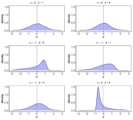
Figure 1. Kernel density curves of six different degrees of non-normal latent variables.

3.2.2. Type 2

We first fix the total number of latent variables at K, which includes both normally and non-normally distributed dimensions. Following Svetina et al. [16] and Wang et al. [17], we simulate varying degrees of non-normality by altering the number of non-normal dimensions from 0 to K. For each non-normal latent variable, we fix $(\alpha =2,\beta =4)$, as this combination represents the greatest deviation from normality as observed in Figure 1.

For example, when $K=3$, the number of non-normal dimensions varies as follows: zero dimensions (non0), the first dimension only (non1), the first two dimensions (non2), and all three dimensions (non3).

4. Simulation Studies

In this section, we compare the robustness of three methods: the improved EMS [26], the accelerated EML1 [6], and EIFA with three oblique rotations (Quartimin, Geomin, and Infomax). In EIFA, a sparse discrimination matrix is obtained by thresholding small discrimination parameter estimates to zero. Note that, selecting a suitable threshold for EIFA is important but nontrivial. In practice, discrimination parameters below 0.30 or 0.32 are often treated as negligible [31,32]. Following this convention, and in line with the specification in Shang et al. [9], we set 0.30 as the threshold in our study. All analyses are conducted using publicly accessible R codes hosted at https://github.com/xupf900/ (accessed on 24 November 2025). Simulations are run on a 64-bit Windows 10 system configured with an Intel(R) Xeon(R) Gold 5118 CPU (2.30 GHz) and 256 GB of RAM.

4.1. Simulation Design

In the simulations, we consider M2PL models with $K=3,5$ latent dimensions, while fixing the number of items at $J=40$. The non-zero elements of the discrimination parameter matrices $\mathit{A}$ are independently drawn from a uniform distribution $U(0.5,2)$. The elements of the vectors $\mathit{b}$ are sampled from the standard normal distribution. The true parameter values for $\mathit{A}$ and $\mathit{b}$ under all scenarios are provided in Section S1 of the Supplementary File.

For the covariance matrix $\mathsf{\Sigma }$ of latent traits, the diagonal elements are fixed at 1, and the off-diagonal elements are set to either 0.4 or 0.6 to represent moderate and higher correlations, respectively. Four sample size levels $N=500,1000,2000,4000$ are considered. To simulate violations of the normality, we consider the following two settings:

Simulation 1. 

Type 1 latent variable distributions are used, with $(\alpha ,\beta )=(-1,0)$ and $(2,4)$ for $K=3$, and $(\alpha ,\beta )=(2,4)$ for $K=5$. The correlation is set to 0.4.

Simulation 2. 

Type 2 latent variable distributions with $(\alpha ,\beta )=(2,4)$ are used for both $K=3$ and $K=5$. The correlation is again set to 0.4.

Under each setting, we draw $Z=200$ independent data sets and apply EMS, EML1, and EIFA with rotations to recover the discrimination parameter matrix. To resolve the issue of rotational indeterminacy, the same identification constraint is applied to EMS and EML1, but not to EIFA with rotations. Specifically, we fix a $K\times K$ submatrix of the discrimination parameter matrix $\mathit{A}$ to be an identity matrix. For example, when $K=3$, items 1, 10, and 19 are constrained to relate only to latent traits 1, 2, and 3, respectively. That is, the structure of ${\left({\mathit{a}}_1,{\mathit{a}}_{10},{\mathit{a}}_{19}\right)}^{\top }$ is fixed to the identity matrix. Similarly, for $K=5$, we fix ${\left({\mathit{a}}_1,{\mathit{a}}_5,{\mathit{a}}_9,{\mathit{a}}_{13},{\mathit{a}}_{17}\right)}^{\top }$ accordingly.

4.2. Evaluation Metrics

This paper evaluates the simulation results using three structural recovery metrics: F1-score, true positive rate (TPR), and false positive rate (FPR). In addition, the mean squared error (MSE) is used to assess parameter estimation.

For each replication z, let ${\widehat{M}}^{\left(z\right)}={\left(I(a_{jk}^{\left(z\right)}\ne 0)\right)}_{J\times K}$, where ${\widehat{a}}_{jk}^{\left(z\right)}$ denotes the estimate of $a_{jk}$. We define the following quantities (excluding entries fixed by identification constraints):

$${\mathrm{TP}}^{\left(z\right)}=\sum _{j,k}I({\widehat{M}}_{jk}^{\left(z\right)}=1,M_{jk}=1),{\mathrm{FP}}^{\left(z\right)}=\sum _{j,k}I({\widehat{M}}_{jk}^{\left(z\right)}=1,M_{jk}=0),$$

$${\mathrm{FN}}^{\left(z\right)}=\sum _{j,k}I({\widehat{M}}_{jk}^{\left(z\right)}=0,M_{jk}=1),{\mathrm{TN}}^{\left(z\right)}=\sum _{j,k}I({\widehat{M}}_{jk}^{\left(z\right)}=0,M_{jk}=0).$$

The precision, TPR (i.e., recall), and FPR for replication z are defined as

$${\mathrm{Precision}}^{\left(z\right)}={\displaystyle \frac{{\mathrm{TP}}^{\left(z\right)}}{{\mathrm{TP}}^{\left(z\right)}+{\mathrm{FP}}^{\left(z\right)}}},{\mathrm{FPR}}^{\left(z\right)}={\displaystyle \frac{{\mathrm{FP}}^{\left(z\right)}}{{\mathrm{FP}}^{\left(z\right)}+{\mathrm{TN}}^{\left(z\right)}}},$$

$${\mathrm{TPR}}^{\left(z\right)}={\mathrm{Recall}}^{\left(z\right)}={\displaystyle \frac{{\mathrm{TP}}^{\left(z\right)}}{{\mathrm{TP}}^{\left(z\right)}+{\mathrm{FN}}^{\left(z\right)}}}.$$

The F1-score, which provides a balanced summary of precision and recall, is computed as

$${\mathrm{F}1\text{-}\mathrm{score}}^{\left(z\right)}={\displaystyle \frac{2·{\mathrm{Precision}}^{\left(z\right)}·{\mathrm{Recall}}^{\left(z\right)}}{{\mathrm{Precision}}^{\left(z\right)}+{\mathrm{Recall}}^{\left(z\right)}}},$$

for the zth replication.

The MSE measures the average of the squares of the errors and is calculated for each parameter $a_{jk}$ as

$$\mathrm{MSE}\left(a_{jk}\right)={\displaystyle \frac{1}{Z}}\sum _{z=1}^Z{\left({\widehat{a}}_{jk}^{\left(z\right)}-a_{jk}\right)}^2,$$

(6)

where $Z=200$ is the total number of replications. The MSE for each parameter $b_j$ in $\mathit{b}$ is computed analogously.

4.3. Results

4.3.1. Results for Simulation 1

This subsection presents results for simulation 1. Table 1 provides the mean and standard deviation (in parentheses) of the F1-score for all methods. From this table, EMS achieves the highest F1-score when the sample size is small ($N=500$) across all normal and non-normal conditions. However, its performance does not improve as N increases; in fact, the F1-score decreases slightly for larger samples, particularly when $K=5$. This decline suggests that EMS may lack asymptotic consistency in recovering the item–trait relationships. In contrast, the performance of EML1 and EIFA with rotations improves steadily with N, indicating stronger large-sample consistency. For $N=1000,2000,4000$, EIFA with rotations consistently outperforms both EMS and EML1. The only exception occurs at $(\alpha ,\beta )=(0,0)$ with $K=3$ and $N=4000$, where EML1 achieves the highest F1-score. Among rotations, Quartimin, Geomin, and Infomax produce very similar results.

Table 1. Mean and standard deviation of the F1-score of $\widehat{M}$ under simulation setting 1, where the correlation coefficient is 0.4.

	K = 3
	N = 500				N = 1000				N = 2000				N = 4000
$(\alpha ,\beta )$	(0,0)	(−1,0)	(2,4)		(0,0)	(−1,0)	(2,4)		(0,0)	(−1,0)	(2,4)		(0,0)	(−1,0)	(2,4)
EMS	0.983	0.978	0.951		0.990	0.984	0.968		0.987	0.977	0.957		0.979	0.963	0.931
	(0.014)	(0.016)	(0.028)		(0.011)	(0.012)	(0.017)		(0.012)	(0.012)	(0.017)		(0.016)	(0.015)	(0.019)
EML1	0.969	0.958	0.940		0.990	0.987	0.967		0.998	0.994	0.979		0.999	0.992	0.980
	(0.018)	(0.019)	(0.025)		(0.010)	(0.011)	(0.016)		(0.005)	(0.008)	(0.013)		(0.003)	(0.011)	(0.012)
Quartimin	0.965	0.962	0.938		0.993	0.990	0.974		0.996	0.998	0.990		0.986	1.000	0.995
	(0.038)	(0.024)	(0.040)		(0.021)	(0.018)	(0.046)		(0.031)	(0.004)	(0.041)		(0.062)	(0.001)	(0.035)
Geomin	0.963	0.957	0.933		0.992	0.988	0.970		0.995	0.998	0.988		0.986	1.000	0.994
	(0.035)	(0.027)	(0.043)		(0.021)	(0.023)	(0.053)		(0.038)	(0.004)	(0.046)		(0.063)	(0.002)	(0.037)
Infomax	0.956	0.949	0.929		0.988	0.983	0.966		0.995	0.996	0.985		0.986	0.999	0.992
	(0.035)	(0.024)	(0.036)		(0.021)	(0.018)	(0.042)		(0.033)	(0.007)	(0.038)		(0.061)	(0.003)	(0.034)
	K = 5
	N = 500				N = 1000				N = 2000				N = 4000
$(\alpha ,\beta )$	(0,0)	(2,4)			(0,0)	(2,4)			(0,0)	(2,4)			(0,0)	(2,4)
EMS	0.952	0.903			0.958	0.934			0.945	0.918			0.922	0.886
	(0.024)	(0.036)			(0.021)	(0.025)			(0.024)	(0.023)			(0.032)	(0.030)
EML1	0.941	0.867			0.978	0.923			0.984	0.942			0.996	0.956
	(0.023)	(0.047)			(0.015)	(0.026)			(0.010)	(0.018)			(0.006)	(0.017)
Quartimin	0.900	0.860			0.967	0.937			0.995	0.970			0.999	0.983
	(0.027)	(0.032)			(0.022)	(0.019)			(0.006)	(0.015)			(0.007)	(0.017)
Geomin	0.906	0.862			0.973	0.944			0.997	0.978			0.999	0.988
	(0.026)	(0.042)			(0.025)	(0.018)			(0.004)	(0.024)			(0.013)	(0.025)
Infomax	0.895	0.855			0.963	0.928			0.993	0.962			0.999	0.976
	(0.028)	(0.033)			(0.023)	(0.018)			(0.007)	(0.023)			(0.007)	(0.020)

Note: The bold formatting is used to highlight the best results.

Regarding the effect of non-normality, all methods show some degradation in F1-score relative to the normal case in most settings. Larger departures from normality generally lead to greater decreases in performance. This trend is particularly evident for the combination $(\alpha ,\beta )=(2,4)$, where most methods achieve their lowest F1-scores. However, for $K=3$ and larger sample sizes ($N=2000$ and $N=4000$), EIFA with rotations shows strong robustness and, in several instances, even benefits from moderate non-normality, achieving an F1-score of 1 in multiple conditions.

Figure 2 shows the boxplots of the MSEs of $\widehat{\mathit{A}}$. Note that these boxplots are based on the $J\times K$ element-wise values of $MSE\left(a_{jk}\right)$ defined in Equation (6). From Figure 2, EMS and EML1 show better estimation of $\mathit{A}$ than EIFA with rotations in most cases, especially when $\alpha =2$ and $\beta =4$. This may be because EMS and EML1 estimate $\mathit{A}$ by directly optimizing penalized likelihoods. In contrast, EIFA uses marginal maximum likelihood followed by rotation and thresholding. The extra cutoff step can introduce small distortions and reduce estimation accuracy. Note that while larger sample sizes generally reduce the MSE of $\widehat{\mathit{A}}$, some non-normal conditions still yield higher MSEs than the normal cases, as shown in Figure 2. Figure 3 shows the boxplots of the MSEs of $\widehat{\mathit{b}}$. Non-normality increases the MSE, and larger sample sizes do not noticeably reduce it. For $(\alpha ,\beta )=(2,4)$, EMS gives the smallest MSE. But for $(\alpha ,\beta )=(-1,0)$, EIFA with rotations performs best. Thus, no method consistently dominates under non-normality. This may be because all three methods estimate $\mathit{b}$ directly through likelihood-based optimization.

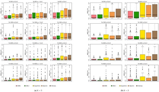
Figure 2. Boxplots of the MSEs of $\widehat{\mathit{A}}$ under simulation 1.

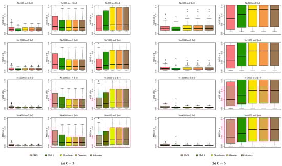
Figure 3. Boxplots of the MSEs of $\widehat{\mathit{b}}$ under simulation 1.

4.3.2. Results for Simulation 2

This subsection presents results from simulation 2. Table 2 reports the mean of F1-scores (with standard deviations) for $\widehat{M}$ under simulation setting 2, where the inter-factor correlation is fixed at $0.4$. A clear pattern emerges as the sample size increases. When $N=500$, EMS achieves the highest F1-scores for both $K=3$ and $K=5$. This is likely because its MS-step minimizes the expected BIC and tends to select a sparse discrimination matrix $\mathit{A}$ that is close to the true M2PL structure. The reduced model complexity improves structural recovery in small samples. However, as the sample size increases, the performance of EMS declines. In contrast, the F1-scores of EML1 and EIFA with rotations steadily increase with N. As a result, EML1 and EIFA with rotations outperform EMS for large N. This pattern implies that EML1 and EIFA with rotations exhibit better consistency properties than EMS.

Table 2. Mean and standard deviation of the F1-score of $\widehat{M}$ under simulation 2.

	K = 3
	N = 500							N = 1000							N = 2000							N = 4000
	non0	non1	non2	non3				non0	non1	non2	non3				non0	non1	non2	non3				non0	non1	non2	non3
EMS	0.983	0.972	0.968	0.951				0.990	0.985	0.980	0.968				0.987	0.985	0.975	0.957				0.979	0.976	0.962	0.931
	(0.014)	(0.016)	(0.020)	(0.028)				(0.011)	(0.013)	(0.014)	(0.017)				(0.012)	(0.013)	(0.016)	(0.017)				(0.016)	(0.017)	(0.022)	(0.019)
EML1	0.969	0.955	0.951	0.940				0.990	0.981	0.977	0.967				0.998	0.993	0.988	0.979				0.999	0.998	0.992	0.980
	(0.018)	(0.021)	(0.022)	(0.025)				(0.010)	(0.013)	(0.013)	(0.016)				(0.005)	(0.008)	(0.011)	(0.013)				(0.003)	(0.005)	(0.009)	(0.012)
Quartimin	0.965	0.962	0.955	0.938				0.993	0.987	0.986	0.974				0.996	0.990	0.996	0.990				0.986	0.993	0.996	0.995
	(0.038)	(0.031)	(0.027)	(0.040)				(0.021)	(0.037)	(0.032)	(0.046)				(0.031)	(0.049)	(0.027)	(0.041)				(0.062)	(0.044)	(0.034)	(0.035)
Geomin	0.963	0.958	0.949	0.933				0.992	0.987	0.984	0.970				0.995	0.990	0.995	0.988				0.986	0.993	0.996	0.994
	(0.035)	(0.033)	(0.030)	(0.043)				(0.021)	(0.040)	(0.036)	(0.053)				(0.038)	(0.049)	(0.029)	(0.046)				(0.063)	(0.045)	(0.034)	(0.037)
Infomax	0.956	0.952	0.946	0.929				0.988	0.982	0.982	0.966				0.995	0.989	0.996	0.985				0.986	0.993	0.995	0.992
	(0.035)	(0.030)	(0.023)	(0.036)				(0.021)	(0.037)	(0.032)	(0.042)				(0.033)	(0.049)	(0.012)	(0.038)				(0.061)	(0.042)	(0.035)	(0.034)
	K = 5
	N = 500							N = 1000							N = 2000							N = 4000
	non0	non1	non2	non3	non4	non5		non0	non1	non2	non3	non4	non5		non0	non1	non2	non3	non4	non5		non0	non1	non2	non3	non4	non5
EMS	0.952	0.918	0.921	0.905	0.905	0.903		0.958	0.957	0.956	0.951	0.942	0.934		0.945	0.956	0.954	0.943	0.937	0.918		0.922	0.937	0.936	0.932	0.917	0.886
	(0.024)	(0.036)	(0.033)	(0.038)	(0.035)	(0.036)		(0.021)	(0.021)	(0.022)	(0.023)	(0.022)	(0.025)		(0.024)	(0.019)	(0.022)	(0.026)	(0.024)	(0.023)		(0.032)	(0.031)	(0.030)	(0.036)	(0.030)	(0.030)
EML1	0.941	0.884	0.885	0.876	0.876	0.867		0.978	0.937	0.933	0.934	0.929	0.923		0.984	0.964	0.959	0.964	0.958	0.942		0.996	0.979	0.975	0.981	0.972	0.956
	(0.023)	(0.040)	(0.042)	(0.044)	(0.043)	(0.047)		(0.015)	(0.029)	(0.026)	(0.025)	(0.024)	(0.026)		(0.010)	(0.019)	(0.019)	(0.018)	(0.018)	(0.018)		(0.006)	(0.015)	(0.014)	(0.013)	(0.014)	(0.017)
Quartimin	0.900	0.897	0.891	0.871	0.866	0.860		0.967	0.963	0.961	0.949	0.942	0.937		0.995	0.990	0.986	0.983	0.976	0.970		0.999	0.992	0.995	0.995	0.989	0.983
	(0.027)	(0.027)	(0.029)	(0.033)	(0.031)	(0.032)		(0.022)	(0.024)	(0.019)	(0.029)	(0.024)	(0.019)		(0.006)	(0.023)	(0.026)	(0.018)	(0.015)	(0.015)		(0.007)	(0.028)	(0.022)	(0.014)	(0.009)	(0.017)
Geomin	0.906	0.902	0.895	0.875	0.867	0.862		0.973	0.968	0.965	0.955	0.949	0.944		0.997	0.991	0.988	0.985	0.981	0.978		0.999	0.990	0.994	0.994	0.992	0.988
	(0.026)	(0.029)	(0.034)	(0.038)	(0.036)	(0.042)		(0.025)	(0.033)	(0.028)	(0.036)	(0.029)	(0.018)		(0.004)	(0.032)	(0.032)	(0.031)	(0.024)	(0.024)		(0.013)	(0.037)	(0.029)	(0.028)	(0.018)	(0.025)
Infomax	0.895	0.891	0.884	0.867	0.860	0.855		0.963	0.961	0.954	0.944	0.937	0.928		0.993	0.986	0.984	0.980	0.973	0.962		0.999	0.991	0.994	0.994	0.985	0.976
	(0.028)	(0.029)	(0.029)	(0.034)	(0.030)	(0.033)		(0.023)	(0.023)	(0.019)	(0.028)	(0.028)	(0.018)		(0.007)	(0.031)	(0.027)	(0.028)	(0.015)	(0.023)		(0.007)	(0.033)	(0.023)	(0.016)	(0.008)	(0.020)

Note: The bold formatting is used to highlight the best results.

In addition, we can see a systematic impact of non-normality from Table 2. As the number of non-normal latent dimensions increases, all methods exhibit a decline in F1-score, especially when $N=500$. However, for large sample sizes, the negative effect of non-normality on EIFA with rotations is minimal. EIFA with rotations remains comparatively robust and continues to achieve F1-scores extremely close to 1. This robustness may stem from the consistency properties that EIFA with rotations enjoys under normality, which appear to extend favorably to mildly non-normal settings.

Figure 4 shows the boxplots of the MSEs of $\widehat{\mathit{A}}$. From this figure, the MSE increases with the number of non-normal latent variables. Overall, EMS and EML1 outperform EIFA with rotations in terms of estimation accuracy. While a larger sample size helps reduce the MSE, it does not fully eliminate the adverse effects of non-normality. This behavior is consistent with the results observed in simulation 1. Figure 5 displays the boxplots of the MSEs of $\widehat{\mathit{b}}$. From Figure 5, all methods perform similarly under normal conditions; yet, EMS and EML1 outperform EIFA with rotations in terms of estimation accuracy for most non-normal cases. Increasing the sample size significantly reduces the MSE of $\widehat{\mathit{b}}$ under both normal and non-normal conditions.

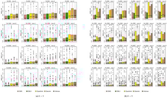
Figure 4. Boxplots of the MSEs of $\widehat{\mathit{A}}$ under simulation 2.

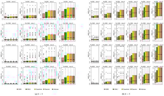
Figure 5. Boxplots of the MSEs of $\widehat{\mathit{b}}$ under simulation 2.

4.4. Additional Simulation Results

As higher inter-factor correlations are common in psychological research, we conduct additional simulation studies using a stronger correlation of 0.6. As expected, this stronger correlation decreases the F1-scores and increases the MSEs. The comparative behaviors of EMS, EML1, and EIFA with rotations remain similar to those observed in simulations 1 and 2. Therefore, these results are moved to the Appendix A to save space in the main paper.

Moreover, we report additional simulation results in the Supplementary File, including the TPR and FPR for $\widehat{\mathit{M}}$, the biases of $\widehat{\mathit{A}}$ and $\widehat{\mathit{b}}$, the MSEs and biases of $\widehat{\mathsf{\Sigma }}$, and the CPU time. From the TPR and FPR results, we observe that when the sample size is large ($N=4000$), EMS attains a TPR close to 1 but also a non-negligible FPR. This leads to poorer F1-score in recovering item–trait relationships. The finding suggests that EMS may require stronger penalization on the likelihood, for example, by employing the extended Bayesian information criterion (EBIC). EBIC is commonly used in high-dimensional settings. Further empirical and theoretical work is needed to explore this direction.

Regarding the effect of skewness, higher skewness results in larger bias in the estimates of the difficulty parameters $\widehat{\mathit{b}}$. In terms of computational cost, EML1 is the slowest method, likely because it must evaluate multiple regularization parameters in (3). EMS is also slower than EIFA with rotations, presumably due to its greater number of iterations. In future work, we plan to adopt the smooth approximation of BIC for regularized estimation proposed by Robitzsch [25] to improve computational efficiency.

5. Real Data Analysis

Psychological constructs such as depression, pain, and gambling are particularly likely to exhibit non-normal distributions in the general population [12]. To illustrate how such non-normal latent traits affect the performance in latent variable selection, we apply the EMS, EML1, and EIFA with rotations to analyze a real data set based on the Depression, Anxiety, and Stress Scale (42-item version, DASS-42) under the M2PL model. The DASS-42 data set, which contains responses from 5000 subjects to 42 items, is publicly available at https://osf.io/ykq2a/ (accessed on 8 May 2025). The items are reordered such that items 1–14, 15–28, and 29–42 correspond to the latent traits of depression (D), anxiety (A), and stress (S), respectively [33]. The full item content and measurement structure are presented in Table A2 in Appendix B. Responses are originally collected on a 4-point scale (0 = “Did not apply to me at all”; 1 = “Applied to me to some degree, or some of the time”; 2 = “Applied to me to a considerable degree, or a good part of time”; 3 = “Applied to me very much, or most of the time”). In our analysis, we dichotomize the responses by retaining 0 as 0 (symptom absence) and recoding categories 1–3 as 1 (symptom presence).

To verify the non-normality of the latent traits involved in this dataset, we compute factor scores by summarizing all responses for each individual on dimensions D, A, and S. As demonstrated in Figure 6 and Table 3, all three latent trait distributions exhibit substantial deviations from normality, thereby confirming the presence of non-normal latent traits in the DASS-42 data.

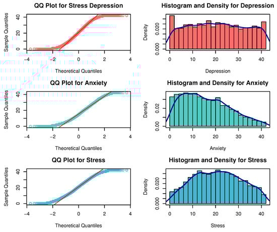
Figure 6. QQ plots, histograms, and density curves for depression, anxiety, and stress.

Table 3. Results of normality tests for depression, anxiety, and stress.

	Shapiro-Wilk			Jarque-Bera
	W	P		JB	P
D	0.9588	<2 $\times {10}^{-16}$		269.348	<2 $\times {10}^{-16}$
A	0.9631	<2 $\times {10}^{-16}$		256.3907	<2 $\times {10}^{-16}$
S	0.9802	<2 $\times {10}^{-16}$		165.5031	<2 $\times {10}^{-16}$

Next, we compare the performance of EMS, EML1, and EIFA with rotations in identifying the item–trait relationships in this dataset. To ensure identifiability, we designate one item for each trait based on the content of the items, similarly as Xu et al. [8]. Specifically, items 1, 15, and 29 are exclusively assigned to traits D, A, and S, respectively. The loading structures estimated by EMS, EML1, and EIFA with rotations are visualized as heatmaps in Figure 7. The estimated $\widehat{\mathit{A}}$ and $\widehat{\mathit{b}}$ are reported in Table A3, Table A4, Table A5, Table A6 and Table A7 in Appendix B, and $\widehat{\mathsf{\Sigma }}$ are

$${\widehat{\mathsf{\Sigma }}}_{EMS}=\left(\begin{array}{ccc}1.000& 0.393& 0.399\\ 0.393& 1.000& 0.507\\ 0.399& 0.507& 1.000\end{array}\right),{\widehat{\mathsf{\Sigma }}}_{EML1}=\left(\begin{array}{ccc}1.000\hfill & 0.457\hfill & 0.520\hfill \\ 0.457\hfill & 1.000\hfill & 0.611\hfill \\ 0.520\hfill & 0.611\hfill & 1.000\hfill \end{array}\right),$$

$${\widehat{\mathsf{\Sigma }}}_{Quartimin}=\left(\begin{array}{ccc}1.000\hfill & 0.601\hfill & 0.652\hfill \\ 0.601\hfill & 1.000\hfill & 0.700\hfill \\ 0.652\hfill & 0.700\hfill & 1.000\hfill \end{array}\right),{\widehat{\mathsf{\Sigma }}}_{Geomin}=\left(\begin{array}{ccc}1.000& 0.574& 0.664\\ 0.574& 1.000& 0.722\\ 0.664& 0.722& 1.000\end{array}\right),$$

$${\widehat{\mathsf{\Sigma }}}_{Infomax}=\left(\begin{array}{ccc}1.000\hfill & 0.672\hfill & 0.750\hfill \\ 0.672\hfill & 1.000\hfill & 0.775\hfill \\ 0.750\hfill & 0.775\hfill & 1.000\hfill \end{array}\right).$$

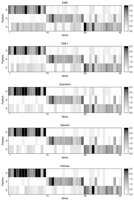
Figure 7. Heatmaps of the loading matrices estimated by EMS, EML1, and EIFA with rotations for the DASS-42 data set.

It can be seen that the estimated correlations among the latent traits are relatively high, with those obtained by EIFA with rotations evidently exceeding those produced by EMS and EML1. This suggests that the constructs are interconnected and mutually influential, even though each DASS-42 item is originally designed to measure a single psychological construct (D, A, or S). In other words, the constructs are not entirely distinct but partially overlapping in their manifestations. For example, items 27 and 33 are found to be associated with both anxiety and stress.

While the designed item–trait relationships serve as the benchmark, it is important to acknowledge that multiple psychological constructs may interact when subjects respond to items. Comparing the estimated loading structures with the benchmark, the F1-scores of EMS, EML1, and EIFA with rotations (Quartimin, Geomin, and Infomax) are 0.582, 0.609, 0.724, 0.724, and 0.706, respectively. Although EIFA with rotations achieves the highest F1-scores and produce the sparsest loading structures, none of the methods attains high accuracy in identifying item–trait relationships under conditions of stronger inter-factor correlations and non-normal latent trait distributions. These findings from the DASS-42 data analysis are consistent with our simulation results.

6. Discussion

This study evaluates the robustness of EMS, EML1, and EIFA with rotations for identifying item–trait relationships under non-normal latent distributions in MIRT models. Our simulation results suggest the following. For identifying item–trait relationships, EMS is preferable for small samples, whereas EIFA with rotations performs better for large samples. For estimation accuracy, EMS and EML1 generally outperform EIFA with rotations. EMS likely achieves higher accuracy because it directly optimizes a penalized likelihood, while EIFA relies on thresholding small loadings, which can reduce precision. A potential improvement is to apply marginal maximum likelihood estimation after thresholding to enhance estimation accuracy.

The simulation results align closely with previous IRT research. Consistent with Svetina et al. [16] and McClure and Jacobucci [18], we also find that higher inter-factor correlations significantly exacerbate the adverse effects of non-normality. When the correlation increases to 0.6, the impact of non-normality on parameter estimation becomes notably stronger than when the correlation is 0.4. Furthermore, consistent with Finch and Edwards [15], McClure and Jacobucci [18], and Wall et al. [34], a large sample size helps reduce, but does not eliminate, estimation errors. These errors remain larger than those under normality, especially when the number of latent traits is five.

To address violations of normality, more robust methods are needed. One direction is to allow flexible latent trait distributions, such as semi-nonparametric forms [35], multivariate skew-normal models [36], or centered skew-t distributions [37]. We plan to extend EMS and EML1 to these distributional frameworks in future work. Another direction is limited-information estimation based on tetrachoric or polychoric correlations. These methods avoid full multivariate integration and depend only on low-order summary statistics, making them faster and less sensitive to distributional assumptions. Inspired by Huang [38], which uses penalized least squares for ordinal structural equation modeling, we will explore regularized limited-information estimation for MIRT.

References

- Bock, R.D.; Gibbons, R.; Muraki, E. Full-information item factor analysis. Appl. Psychol. Meas. 1988, 12, 261–280. [Google Scholar] [CrossRef]
- Cai, L. High-dimensional exploratory item factor analysis by a Metropolis–Hastings Robbins–Monro algorithm. Psychometrika 2010, 75, 33–57. [Google Scholar] [CrossRef]
- Browne, M.W. An overview of analytic rotation in exploratory factor analysis. Multivar. Behav. Res. 2001, 36, 111–150. [Google Scholar] [CrossRef]
- Sun, J.; Chen, Y.; Liu, J.; Ying, Z.; Xin, T. Latent variable selection for multidimensional item response theory models via L1 regularization. Psychometrika 2016, 81, 921–939. [Google Scholar] [CrossRef] [PubMed]
- Zhang, S.; Chen, Y. Computation for latent variable model estimation: A unified stochastic proximal framework. Psychometrika 2022, 87, 1473–1502. [Google Scholar] [CrossRef]
- Shang, L.; Xu, P.F.; Shan, N.; Tang, M.L.; Ho, G.T.S. Accelerating L1-penalized expectation maximization algorithm for latent variable selection in multidimensional two-parameter logistic models. PLoS ONE 2023, 18, e0279918. [Google Scholar] [CrossRef]
- Schwarz, G. Estimating the Dimension of a Model. Ann. Stat. 1978, 6, 461–464. [Google Scholar] [CrossRef]
- Xu, P.F.; Shang, L.; Zheng, Q.Z.; Shan, N.; Tang, M.L. Latent variable selection in multidimensional item response theory models using the expectation model selection algorithm. Br. J. Math. Stat. Psychol. 2022, 75, 363–394. [Google Scholar] [CrossRef]
- Shang, L.; Zheng, Q.Z.; Xu, P.F.; Tang, M.L. A generalized expectation model selection algorithm for latent variable selection in multidimensional item response theory models. Stat. Comput. 2024, 34, 49. [Google Scholar] [CrossRef]
- Wall, M.M.; Park, J.Y.; Moustaki, I. IRT modeling in the presence of zero-inflation with application to psychiatric disorder severity. Appl. Psychol. Meas. 2015, 39, 583–597. [Google Scholar] [CrossRef] [PubMed]
- Woods, C.M.; Thissen, D. Item response theory with estimation of the latent population distribution using spline-based densities. Psychometrika 2006, 71, 281–301. [Google Scholar] [CrossRef]
- Preston, K.S.J.; Reise, S.P. Estimating the nominal response model under nonnormal conditions. Educ. Psychol. Meas. 2014, 74, 377–399. [Google Scholar] [CrossRef]
- Sass, D.A.; Schmitt, T.A.; Walker, C.M. Estimating non-normal latent trait distributions within item response theory using true and estimated item parameters. Appl. Meas. Educ. 2008, 21, 65–88. [Google Scholar] [CrossRef]
- Stone, C.A. Recovery of marginal maximum likelihood estimation in the two-parameter logistic model: An evaluation of MULTILOG. Appl. Psychol. Meas. 1992, 16, 1–16. [Google Scholar] [CrossRef]
- Finch, H.; Edwards, J.M. Rasch model parameter estimation in the presence of a nonnormal latent trait using a nonparametric Bayesian approach. Educ. Psychol. Meas. 2016, 76, 662–684. [Google Scholar] [CrossRef]
- Svetina, D.; Valdivia, A.; Underhill, S.; Dai, S.; Wang, X. Parameter recovery in multidimensional item response theory models under complexity and nonnormality. Appl. Psychol. Meas. 2017, 41, 530–544. [Google Scholar] [CrossRef] [PubMed]
- Wang, C.; Su, S.; Weiss, D.J. Robustness of parameter estimation to assumptions of normality in the multidimensional graded response model. Multivar. Behav. Res. 2018, 53, 403–418. [Google Scholar] [CrossRef] [PubMed]
- McClure, K.; Jacobucci, R. Item parameter calibration in the multidimensional graded response model with high dimensional tests. PsyArXiv 2023. [Google Scholar] [CrossRef]
- Vale, C.D.; Maurelli, V.A. Simulating multivariate nonnormal distributions. Psychometrika 1983, 48, 465–471. [Google Scholar] [CrossRef]
- Astivia, O.L.O.; Zumbo, B.D. A cautionary note on the use of the Vale and Maurelli method to generate multivariate, nonnormal data for simulation purposes. Educ. Psychol. Meas. 2015, 75, 541–567. [Google Scholar] [CrossRef]
- Foldnes, N.; Grønneberg, S. How general is the Vale–Maurelli simulation approach? Psychometrika 2015, 80, 1066–1083. [Google Scholar] [CrossRef]
- Foldnes, N.; Olsson, U.H. A simple simulation technique for nonnormal data with prespecified skewness, kurtosis, and covariance matrix. Multivar. Behav. Res. 2016, 51, 207–219. [Google Scholar] [CrossRef]
- Carroll, J.B. An analytical solution for approximating simple structure in factor analysis. Psychometrika 1953, 18, 23–38. [Google Scholar] [CrossRef]
- Clarkson, D.B.; Jennrich, R.I. Quartic rotation criteria and algorithms. Psychometrika 1988, 53, 251–259. [Google Scholar] [CrossRef]
- Robitzsch, A. Smooth information criterion for regularized estimation of item response models. Algorithms 2024, 17, 153. [Google Scholar] [CrossRef]
- Shang, L.; Xu, P.F.; Shan, N.; Tang, M.L.; Zheng, Q.Z. The improved EMS algorithm for latent variable selection in M3PL model. Appl. Psychol. Meas. 2025, 49, 50–70. [Google Scholar] [CrossRef] [PubMed]
- Dempster, A.P.; Laird, N.M.; Rubin, D.B. Maximum likelihood from incomplete data via the EM algorithm. J. R. Stat. Soc. Ser. B (Methodol.) 1977, 39, 1–22. [Google Scholar] [CrossRef]
- Jiang, J.; Nguyen, T.; Rao, J.S. The E-MS algorithm: Model selection with incomplete data. J. Am. Stat. Assoc. 2015, 110, 1136–1147. [Google Scholar] [CrossRef]
- Grønneberg, S.; Foldnes, N.; Marcoulides, K.M. covsim: An R package for simulating non-normal data for structural equation models using copulas. J. Stat. Softw. 2022, 102, 1–45. [Google Scholar] [CrossRef]
- Curran, P.J.; West, S.G.; Finch, J.F. The robustness of test statistics to nonnormality and specification error in confirmatory factor analysis. Psychol. Methods 1996, 1, 16–29. [Google Scholar] [CrossRef]
- Hair, J.; Black, W.C.; Anderson, R.E. Multivariate Data Analysis, 7th ed.; Prentice Hall: Upper Saddle River, NJ, USA, 2010. [Google Scholar]
- Tabachnick, B.G.; Fidell, L.S. Using Multivariate Statistics; Allyn and Bacon: Boston, MA, USA, 2001. [Google Scholar]
- Lovibond, P.F.; Lovibond, S.H. The structure of negative emotional states: Comparison of the Depression Anxiety Stress Scales (DASS) with the Beck Depression and Anxiety Inventories. Behav. Res. Ther. 1995, 33, 335–343. [Google Scholar] [CrossRef] [PubMed]
- Wall, M.M.; Guo, J.; Amemiya, Y. Mixture factor analysis for approximating a nonnormally distributed continuous latent factor with continuous and dichotomous observed variables. Multivar. Behav. Res. 2012, 47, 276–313. [Google Scholar] [CrossRef] [PubMed]
- Monroe, S.L. Multidimensional Item Factor Analysis with Semi-Nonparametric Latent Densities. Ph.D. Thesis, University of California, Berkeley, CA, USA, 2014. [Google Scholar]
- Padilla, J.L.; Azevedo, C.L.; Lachos, V.H. Multidimensional multiple group IRT models with skew normal latent trait distributions. J. Multivar. Anal. 2018, 167, 250–268. [Google Scholar] [CrossRef]
- Gómez, J.L.P. Bayesian Inference for Multidimensional Item Response Models Under Heavy Tail Skewed Latent Trait Distributions and Link Functions. Ph.D. Thesis, Universidade Estadual de Campinas, Campinas, Brazil, 2018. [Google Scholar]
- Huang, P.H. Penalized least squares for structural equation modeling with ordinal responses. Multivar. Behav. Res. 2022, 57, 279–297. [Google Scholar] [CrossRef] [PubMed]
Disclaimer/Publisher’s Note: The statements, opinions and data contained in all publications are solely those of the individual author(s) and contributor(s) and not of MDPI and/or the editor(s). MDPI and/or the editor(s) disclaim responsibility for any injury to people or property resulting from any ideas, methods, instructions or products referred to in the content. |
© 2025 by the authors. Licensee MDPI, Basel, Switzerland. This article is an open access article distributed under the terms and conditions of the Creative Commons Attribution (CC BY) license (https://creativecommons.org/licenses/by/4.0/).