Hybrid Partial-Data-Driven H_∞ Robust Tracking Control for Linear Stochastic Systems with Discrete-Time Observation of Reference Trajectory

Abstract

A hybrid robust $H_{\infty }$ tracking-control design method is studied for linear stochastic systems in which the parameters of the reference system are unknown but inferred from discrete-time observations. First, the reference system parameters are estimated by the least-squares method, and a corresponding data-dependent augmented system is constructed. Second, a Riccati matrix inequality is established for these systems, and a state-feedback $H_{\infty }$ controller is designed to improve tracking performance. Third, to mitigate large tracking errors, an error-feedback control scheme is introduced to compensate for dynamic tracking deviations. These results yield a hybrid control framework that integrates data observation, state-feedback $H_{\infty }$ control, and error-feedback $H_{\infty }$ control to address the tracking problem more effectively. Two numerical examples and one practical example demonstrate the effectiveness of the proposed method.

1. Introduction

With advancements in artificial intelligence and data-acquisition technology, data-driven control has become a prominent paradigm in control engineering [1]. Numerous important results have emerged. For instance, Shen et al. studied iterative learning control (ILC) for discrete-time linear systems without prior probability information on randomly varying iteration length [2]. The authors of Ref. [3] proposed a proportional–integral–derivative (PID) control scheme based on adaptive updating rules and data-driven techniques. In [4], bounded-input bounded-output stability, monotonic convergence of tracking-error dynamics, and internal stability of the full-form dynamic-linearization-based model-free adaptive control (MFAC) scheme were analyzed using the contraction mapping principle. The authors of [5] proposed a data-driven adaptive control method based on the incremental triangular dynamic-linearization data model. Recently, data-driven modeling methods have advanced rapidly, yielding notable results in several areas, including predictive control for switched linear systems [6], predictive control for a modular multilevel converter [7], optimal output tracking control [8], self-triggered control [9], and distributed predictive control [10].

The $H_{\infty }$ control technique is an effective method for enhancing robustness against exogenous disturbances [11] and has been widely applied in aerospace, robotics, and wireless communications [12,13,14,15]. Robust $H_{\infty }$ control theory has evolved over more than 40 years. The foundational works include [16,17], which introduce the frequency-domain and algebraic Riccati equation (ARE) methods, respectively, for linear deterministic systems. The linear matrix inequality (LMI) approach was later developed in [18]. For systems subject to random noise [19], stochastic differential equations have been adopted [20], and corresponding $H_{\infty }$ results have been extended to linear Itô systems [21]. $H_{\infty }$ control theories for nonlinear systems have also been established, such as those in [22] for deterministic settings and those in [23]. State-feedback $H_{\infty }$ control for affine stochastic Itô systems was studied in [24] using the completing-squares method. More recently, we proposed an $H_{\infty }$ control design method for general nonlinear discrete-time stochastic systems using the disintegration property of conditional expectation and convex functions [25]. Additional results on $H_{\infty }$ control can be found in [26,27,28] and the references therein.

Tracking-control design techniques are widely used in autonomous underwater vehicles (AUVs), unmanned surface vehicles, and unmanned aerial vehicles (UAVs). For example, Ref. [29] investigated trajectory-tracking control for underactuated autonomous underwater vehicles subject to input constraints and arbitrary attitude maneuvers. A delay-compensated control framework with prescribed performance guarantees was proposed in [30] for trajectory-tracking control of unmanned underwater vehicles (UUVs) subject to uncertain time-varying input delays. The distributed model-predictive control (MPC) framework in [31] was designed for tracking-control problems involving multiple unmanned aerial vehicles (UAVs) interconnected through a directed communication graph. To address size-related limitations in computing invariant sets and to simplify the offline model-predictive control (MPC) design, the authors of Ref. [32] developed an MPC technique based on implicit terminal components. Optimal $H_{\infty }$ adaptive fuzzy observer-based indirect reference tracking-control designs were investigated in [33] for uncertain SISO and MIMO nonlinear stochastic systems with nonlinear uncertain measurement functions and measurement noise.

This paper investigates a hybrid partial-data-driven $H_{\infty }$ robust tracking-control method for the following linear stochastic system to be controlled:

$$dx\left(t\right)=[Ax\left(t\right)+Bu\left(t\right)+B_1{v}_1\left(t\right)]dt+[A_{1}x\left(t\right)+B_2{v}_2\left(t\right)]dW\left(t\right),t\in [t_0,T_f],$$

together with the unknown reference model:

$${\dot{x}}_r\left(t\right)=A_r{x}_r\left(t\right)+v_3\left(t\right),$$

where $x\left(t\right)$ is the system state, $x_r\left(t\right)$ is the reference trajectory, $u\left(t\right)\in {\mathbb{R}}^{n_u}$ is the control input, and $v_1\left(t\right)$, $v_2\left(t\right)$ and $v_3\left(t\right)$ are the exogenous disturbances. The matrices $A,B,B_1,A_1$, and $B_2$ of the system to be controlled are known, whereas the matrix $A_r$ of the reference system is unknown. Only some discrete-time observations of $x_r\left(t\right)$ are available in $t=t_0,t_1,\cdots ,t_N$. To reduce the tracking error, i.e., the distance between $x\left(t\right)$ and $x_r\left(t\right)$, the control input $u\left(t\right)$ must be properly designed.

A data-dependent augmented system is constructed, and state-feedback and error-feedback $H_{\infty }$ controllers are developed accordingly. The resulting hybrid partial-data-driven $H_{\infty }$ control design scheme comprises three stages: data observation, state-feedback $H_{\infty }$ control, and error-feedback $H_{\infty }$ control. In the first stage, information on $x_r\left(t\right)$ is obtained, the reference system parameters are estimated, and the corresponding data-dependent augmented system is constructed, from which a state-feedback $H_{\infty }$ controller is derived. In the second stage, under the action of the state-feedback controller, the tracking error is reduced, although its magnitude remains relatively large because the control depends only on the system state and does not incorporate tracking-error values. In the third stage, an error-feedback $H_{\infty }$ controller is designed to further reduce the tracking error.

Compared with the method of [33], the proposed approach has two main innovations:

• Tracking errors are incorporated not only in the performance index but also directly in the control input through an error-feedback term.
• The control input $u\left(t\right)$ is a hybrid partial-data-driven controller with a piecewise structure.

This paper is organized as follows: In Section 2, some results on $H_{\infty }$ control for linear stochastic systems are reviewed. In Section 3, the data-dependent augmented system is constructed, and the corresponding state-feedback $H_{\infty }$ control and error-feedback $H_{\infty }$ control design methods are studied by solving algebraic Riccati inequalities. In Section 4, the hybrid control scheme is proposed, which includes three stages, and the corresponding programming evolution is also provided. In Section 5, two numerical examples and one practical example are discussed to illustrate the effectiveness of the proposed method.

Notations: $A^T$: the transpose of the matrix A; $\left|x\right|$: the Euclidean norm of the vector $x\in {\mathbb{R}}^n$; $\mathrm{tr}\left(A\right)$: the trace of square matrix $A=\left(a_{ij}\right)\in {\mathbb{R}}^{n\times n}$ with $\mathrm{tr}\left(A\right)={\displaystyle \sum _{i=1}^n}{a}_{ii}$; $\parallel M\parallel$: the norm of matrix $M\in {\mathbb{R}}^{m\times n}$ defined by $\parallel M\parallel =\sqrt{\mathrm{tr}\left(M^{T}M\right)}$; $n_y$: the dimension of vector $y\in {\mathbb{R}}^{n_y}$; $S^n\left(\mathbb{R}\right)$: the set of the n-order real symmetric matrix; $S_{+}^n\left(\mathbb{R}\right)$: the set of the n-order positive definite matrix; $M>0(M\ge 0)$: the matrix M is a positive definite (semi-definite) matrix; $M^{\frac{1}{2}}$: the square root of a positive definite (semi-definite) matrix M; i.e., $M^{\frac{1}{2}}$ is a positive (semi-definite) matrix satisfying $M=M^{\frac{1}{2}}{M}^{\frac{1}{2}}$. ${\parallel v\parallel }_M$: the norm of vector $v\in {\mathbb{R}}^{n_v}$ with weighted matrix M defined by ${\parallel v\parallel }_M=v^{T}Mv$, where $M>0$.

2. Preliminaries

Let $\left\{W\right(t),t\ge 0\}$ be a 1-dimensional standard Brownian motion in a completed probability space $(\mathrm{\Omega },\mathcal{F},\mathbb{F},\mathbb{P})$ with $E\left[W\right(t\left)\right]=0$ and $E\left[W{\left(t\right)}^2\right]=t$. The filtration $\mathbb{F}=\{{\mathcal{F}}_t,t\ge 0\}$ satisfies the usual conditions, and ${\mathcal{F}}_t$ is generated by Brownian motion, i.e.,

$${\mathcal{F}}_t=\sigma \{W_s:0\le s\le t\}\bigvee \mathcal{N}$$

where $\mathcal{N}$ is the totality of $\mathbb{P}$-null sets. Denote $L^2(\mathrm{\Omega },{\mathcal{F}}_t,\mathbb{P};{\mathbb{R}}^n)$ as the set of random variables $\xi$, where $\xi$ is ${\mathcal{F}}_t$-measurable and

$$\mathbb{E}\left[\right|\xi {|}^2]<\infty .$$

Denote ${\mathcal{M}}_{\mathbb{F}}^2([t_0,T_f];{\mathbb{R}}^{n_y})$ as the set of $\mathbb{F}$-adapted stochastic processes $y=\{y_t,t_0\le t\le T_f\}$ with norm

$${\parallel y\parallel }_{{\mathcal{M}}_{\mathbb{F}}^2([t_0,T_f];{\mathbb{R}}^{n_y})}=\sqrt{\mathbb{E}{\int }_{t_0}^{T_f}{\left|y_t\right|}^{2}dt}<\infty .$$

The stochastic linear system with exogenous disturbance $v\left(t\right)$ is given as

$$\left\{\begin{array}{c}dx\left(t\right)=(Ax\left(t\right)+B_{1}v\left(t\right))dt+(A_{1}x\left(t\right)+B_{2}v\left(t\right))dW\left(t\right)\hfill \\ x\left(t_0\right)=x_0\in {\mathbb{R}}^n,t\in [t_0,T_f]\hfill \end{array}.\right.$$

(1)

where $A,A_1\in {\mathbb{R}}^{n\times n}$, $B_1,B_2\in {\mathbb{R}}^{n\times n_v}$ are coefficient matrices, $v\left(t\right)\in {\mathbb{R}}^{n_v}$ is the exogenous disturbance, and $T_f$ is the terminal time with $0<T_f<\infty$. We first review some results of $H_{\infty }$ problem for system (1) that will be used later.

Denote $x(t;v,t_0,x_0)$ the solutions of (1) beginning at $t_0$ with initial state $x_0$ under exogenous disturbance $v=\{v\left(t\right),t_0\le t\le T_f\}$. For every $v\left(t\right)\in {\mathcal{M}}_{\mathbb{F}}^2([t_N,T_f];{\mathbb{R}}^{n_v})$, let

$$z(t;v,t_0,x_0)=Cx(t;v,t_0,x_0)+Dv\left(t\right)$$

be the output of system (1). Define operator $\mathcal{L}:{\mathcal{M}}_{\mathbb{F}}^2([t_0,T_f];{\mathbb{R}}^{n_v})\mapsto {\mathcal{M}}_{\mathbb{F}}^2([t_0,T_f];{\mathbb{R}}^{n_z})$ with

$$\mathcal{L}\left(v\right)=z,$$

where $z\left(t\right)=z(t;v,t_0,0)$. The $H_{\infty }$ norm of $\mathcal{L}$ is defined as

$$\parallel \mathcal{L}\parallel =\underset{v\ne 0}{sup}{\displaystyle \frac{{\parallel z\parallel }_{{\mathcal{M}}_{\mathbb{F}}^2([t_0,T_f];{\mathbb{R}}^{n_z})}}{{\parallel v\parallel }_{{\mathcal{M}}_{\mathbb{F}}^2([t_0,T_f];{\mathbb{R}}^{n_v})}}}.$$

If there exists a constant $\rho >0$ such that, for every $v\left(t\right)\in {\mathcal{M}}_{\mathbb{F}}^2([t_0,T_f];{\mathbb{R}}^{n_v})$,

$${\parallel z\parallel }_{{\mathcal{M}}_{\mathbb{F}}^2([t_0,T_f];{\mathbb{R}}^{n_z})}\le \rho {\parallel v\parallel }_{{\mathcal{M}}_{\mathbb{F}}^2([t_0,T_f];{\mathbb{R}}^{n_v})},$$

(2)

i.e.,

$$\mathbb{E}{\int }_{t_0}^{T_f}{\left|z\left(t\right)\right|}^{2}dt\le {\rho }^2\mathbb{E}{\int }_{t_0}^{T_f}{\left|v\left(t\right)\right|}^{2}dt,$$

(3)

then (2) and (3) are equivalent to

$$\parallel \mathcal{L}\parallel \le \rho .$$

The following lemma is the bounded real lemma from [34], which is also suitable for the case of $H_{\infty }$ problem for system (1).

Lemma 1. 

For some given positive scalar $\rho >0$, suppose there exists a positive definite matrix $P\in {\mathcal{S}}_{+}^n\left(\mathbb{R}\right)$ such that

$$\left[\begin{array}{ccc}PA+A^{T}P+A_1^{T}P{A}_1& P{B}_1+A_1^{T}P{B}_2& C^T\\ ★& -({\rho }^{2}I-B_{2}P{B}_2)& D^T\\ ★& ★& -I\end{array}\right]\le 0,$$

(4)

where ★ denotes the symmetrical part, and then $\parallel \mathcal{L}\parallel \le \rho$. Moreover, there also exists

$$\mathbb{E}{\int }_{t_0}^{T_f}|z(t;t_0,v,\xi ){|}^{2}dt\le \mathbb{E}\left[x_0^{T}P{x}_0\right]+{\rho }^2\mathbb{E}{\int }_{t_0}^{T_f}{\left|v\left(t\right)\right|}^{2}dt,$$

for all $x_0\in {\mathbb{R}}^n$ and $v\left(t\right)\in {\mathcal{M}}_{\mathbb{F}}^2([t_0,T_f];{\mathbb{R}}^{n_v})$.

3. State-Feedback and Error-Feedback ${\mathit{H}}_{\infty }$ Tracking Control for Linear Systems Based on Partially Observable Data

The following linear control systems are considered:

$$\left\{\begin{array}{c}dx\left(t\right)=[Ax\left(t\right)+Bu\left(t\right)+B_1{v}_1\left(t\right)]dt+[A_{1}x\left(t\right)+B_2{v}_2\left(t\right)]dW\left(t\right),\hfill \\ x\left(0\right)=x_0\in {\mathbb{R}}^n,t\in [0,T_f],\hfill \end{array}\right.$$

(5)

where $A,A_1\in {\mathbb{R}}^{n\times n}$, $B\in {\mathbb{R}}^{n\times n_u}$, $B_1\in {\mathbb{R}}^{n\times n_{v_1}}$, $B_2\in {\mathbb{R}}^{n\times n_{v_2}}$, $C\in {\mathbb{R}}^{n_z\times n}$, and $D\in {\mathbb{R}}^{n_z\times n}$ are coefficient matrices, $x\left(t\right)\in {\mathbb{R}}^n$ is the system state, $u\left(t\right)\in {\mathbb{R}}^{n_u}$ is the controller, and $v_1\left(t\right)\in {\mathbb{R}}^{n_{v_1}}$ and $v_2\left(t\right)\in {\mathbb{R}}^{n_{v_2}}$ are the exogenous disturbances.

Suppose the tracking target of system (5) can be described by the following reference model:

$${\dot{x}}_r\left(t\right)=A_r{x}_r\left(t\right)+v_3\left(t\right),$$

(6)

where $x_r\left(t\right)\in {\mathbb{R}}^n$ is the desired reference state tracked by $x\left(t\right)$ in (5), $A_r\in {\mathbb{R}}^{n\times n}$ is the coefficient matrix, and $v_2\left(t\right)\in {\mathbb{R}}^{n_{v_2}}$ is the exogenous disturbance of reference system (6). In system (6), the system coefficient $A_r$ is unknown, but $x_r\left(t\right)$ can be observed at discrete-time $t_0,t_1,\cdots ,t_N$ with $t_0<t_1<\cdots <t_N\le T_f$; i.e., the observation values of $x_r\left(t_0\right),x_r\left(t_1\right),\cdots x_r\left(t_N\right)$ can be obtained.

Denote $e_r\left(t\right)$ as the tracking errors between $x\left(t\right)$ and $x_r\left(t\right)$; i.e.,

$$e_r\left(t\right)=x\left(t\right)-x_r\left(t\right).$$

Our target is, with the background of reference system coefficients unknown and only based on the obtained discrete-time observation $x_r\left(t_0\right),x_r\left(t_1\right),\cdots x_r\left(t_N\right)$, to find an $H_{\infty }$ controller $u\left(t\right)$ such that, for the given $\rho >0$, the tracking performance always satisfies the following inequality in the next coming time $[t_N,T_f]$ given as

$${\int }_{t_N}^{T_f}\mathbb{E}[e_r^T\left(t\right)Q{e}_r\left(t\right)+u^T\left(t\right)Ru\left(t\right)]dt\le {\rho }^2{\int }_{t_N}^{T_f}\mathbb{E}\left[v^T\left(t\right)v\left(t\right)\right]dt,$$

(7)

for all exogenous disturbances $v\left(t\right)={[v_1{\left(t\right)}^T,v_2{\left(t\right)}^T,v_3{\left(t\right)}^T]}^T\in {\mathcal{M}}_{\mathbb{F}}^2([t_N,T_f];{\mathbb{R}}^{n_v})$, where $Q\ge 0$ is the weighted matrix of tracking errors $e\left(t\right)$, $R>0$ is the weighted matrix of controller $u\left(t\right)$, $T_f>0$ is the terminal time of control, and $\rho$ is the attenuation level of external interference on the system.

Denote

$${\xi }_r\left(t_k\right)={\displaystyle \frac{x_r\left(t_{k+1}\right)-x_r\left(t_k\right)}{t_{k+1}-t_k}},k=0,1,\cdots ,N-1.$$

In order to obtain the $H_{\infty }$ control $u\left(t\right)$, the unknown coefficient matrix $A_r$ in system (6) should be estimated first. Because the trajectory $x_r\left(t\right)$ of reference system (6) can be observed at discrete-time $t_0,t_1,\cdots ,t_N$, in order to overcome the system’s uncertainty regarding (6), the observation values of $x_r\left(t_0\right),x_r\left(t_1\right),\cdots x_r\left(t_N\right)$ are used to estimate the unknown matrix $A_r$. This requires the discrete form of (6) as follows:

$${\displaystyle \frac{x_r\left(t_{k+1}\right)-x_r\left(t_k\right)}{t_{k+1}-t_k}}=A_r{x}_r\left(t_k\right)+{ϵ}_k,k=0,1,2,\cdots ,N-1,$$

i.e.,

$${\xi }_r\left(t_k\right)=A_r{x}_r\left(t_k\right)+{ϵ}_k,k=0,1,2,\cdots ,N-1,$$

(8)

where $\{{ϵ}_k,k=0,1,\cdots ,N-1\}$ are the fitting errors or residuals of this model. The least-squares method is used to estimate matrix $A_r$, which satisfies

$${\widehat{A}}_r=arg\underset{A_r}{min}\mathrm{TSSE}\left(A_r\right),$$

(9)

where TSSE is the total sum of squared errors with

$$\mathrm{TSSE}\left(A_r\right)=\sum _{k=0}^{N-1}{\left|{ϵ}_k\right|}^2.$$

(10)

Theorem 1. 

Let $X_r=[x_r\left(t_0\right),x_r\left(t_1\right),\cdots x_r\left(t_{N-1}\right)]$ and ${\mathrm{\Xi }}_r=[{\xi }_r\left(t_0\right),{\xi }_r\left(t_1\right),\cdots {\xi }_r\left(t_{N-1}\right)]$; then, the least-squares estimator of matrix $A_r$ can be presented by

$${\widehat{A}}_r={\mathrm{\Xi }}_r{X}_r^T{\left(X_r{X}_r^T\right)}^{†}.$$

(11)

which satisfies (9), where ${\left(X_r{X}_r^T\right)}^{†}$ is the Moore–Penrose inverse matrix of $X_r{X}_r^T$.

Proof. 

Applying the discrete-time model (8), we can obtain

$${ϵ}_k={\xi }_r\left(t_k\right)-A_{r}x\left(t_k\right),k=0,1,2,\cdots ,N-1.$$

By the definition of $\mathrm{TSSE}\left(A_r\right)$, there exists

$$\begin{array}{cc}\hfill \mathrm{TSSE}\left(A_r\right)& =\sum _{k=0}^{N-1}[{\xi }_r\left(t_k\right)-A_r{x}_{(}{t}_k){]}^T[{\xi }_r\left(t_k\right)-A_r{x}_{(}{t}_k)]\hfill \\ & =tr\left(({\mathrm{\Xi }}_r^T-X_r^T{A}_r^T)({\mathrm{\Xi }}_r-A_r{X}_r)\right)\hfill \\ & =\parallel {\mathrm{\Xi }}_r-A_r{X}_r{\parallel }^2.\hfill \end{array}$$

So, the least-squares estimator of $A_r$ is given by (11). □

Remark 1. 

In Theorem 1, the Moore–Penrose inverse matrix is used. As proposed by the anonymous reviewer, the Moore–Penrose procedure is insufficient. But, if the sample size $N+1$ is large enough, the matrix $X_r{X}_r^T$ can be an invertible matrix, which is shown in Examples 1 and 2. If $X_r{X}_r^T$ is invertible, then it is equivalent to $R\left(X_r{X}_r^T\right)=n$, where $R\left(X_r{X}_r^T\right)$ denotes the rank of matrix $X_r{X}_r^T$. Because $R\left(X_r{X}_r^T\right)\le R\left(X_r\right)$ and $X_r$ is $n\times N$ matrix, the necessary condition for $X_r{X}_r^T$ to be invertible is $N\ge n$. So, if $X_r{X}_r^T$ is invertible, the result of (11) can be replaced by

$$\widehat{A_r}={\mathrm{\Xi }}_r{X}_r^T{\left(X_r{X}_r^T\right)}^{-1}.$$

So, based on the results of Theorem 1, the parameter-unknown reference system (6) can be estimated with the observed data form

$${\dot{x}}_r\left(t\right)={\mathrm{\Xi }}_r{X}_r^T{\left(X_r{X}_r^T\right)}^{†}{x}_r\left(t\right)+v_3\left(t\right).$$

(12)

The augment system of (5) and (12) is written by

$$\left\{\begin{array}{c}d\tilde{x}\left(t\right)=[\tilde{A}\tilde{x}\left(t\right)+\tilde{B}u\left(t\right)+{\tilde{B}}_{1}v\left(t\right)]dt+[\widetilde{A_1}\tilde{x}\left(t\right)+{\tilde{B}}_{2}v\left(t\right)]dW\left(t\right)\hfill \\ \tilde{x}\left(t_N\right)=\left[\begin{array}{c}x\left(t_N\right)\\ x_r\left(t_N\right)\end{array}\right],t\in [t_N,T_f]\hfill \end{array}\right.$$

(13)

where

$$\tilde{x}\left(t\right)=\left[\begin{array}{c}x\left(t\right)\\ x_r\left(t\right)\end{array}\right], v\left(t\right)=\left[\begin{array}{c}{v}_1\left(t\right)\\ v_2\left(t\right)\\ v_3\left(t\right)\end{array}\right], \tilde{A}=\left[\begin{array}{cc}A& 0\\ 0& {\mathrm{\Xi }}_r{X}_r^T{\left(X_r{X}_r^T\right)}^{†}\end{array}\right], \tilde{B}=\left[\begin{array}{c}B\\ 0\end{array}\right],$$

$$\widetilde{A_1}=\left[\begin{array}{cc}{A}_1& 0\\ 0& 0\end{array}\right], {\tilde{B}}_1=\left[\begin{array}{ccc}{B}_1& 0& 0\\ 0& 0& I_{n_{v_3}}\end{array}\right], {\tilde{B}}_2=\left[\begin{array}{ccc}0& B_2& 0\\ 0& 0& 0\end{array}\right].$$

So, the corresponding performance of (13) is rewritten as

$${\int }_{t_N}^{T_f}\mathbb{E}[{\tilde{x}}^T\left(t\right)\tilde{Q}\tilde{x}\left(t\right)+u^T\left(t\right)Ru\left(t\right)]dt\le {\rho }^2{\int }_{t_N}^{T_f}\mathbb{E}\left[v^T\left(t\right)v\left(t\right)\right]dt$$

(14)

where

$$\tilde{Q}=\left[\begin{array}{cc}Q& -Q\\ -Q& Q\end{array}\right].$$

Remark 2. 

Denote the observations of the reference system (6) at discrete-time $t_0,t_1,\cdots ,t_N$ as

$$\mathcal{X}=[x_r\left(t_0\right),x_r\left(t_1\right),\cdots x_r\left(t_N\right)],$$

(15)

and then the coefficients of ${\mathrm{\Xi }}_r$ and $X_r$ in (12) depend on such observation data ${\mathcal{X}}_r$. So, some coefficients of the augment system (13) such as $\tilde{A}$ are also data-dependent where the data ${\mathcal{X}}_r$ is only the observations of $x_r\left(t\right)$ at discrete-time $t_0,t_1,\cdots ,t_N$. Because such data ${\mathcal{X}}_r$ is only the observation of reference system (6) but not including the to-be-controlled system (5), and ${\mathcal{X}}_r$ is only the data at discrete time at $t_0,t_1,\cdots ,t_N$ but not the continuous interval in $[t_0,t_N]$, so the to-be-designed control is called partial-data-driven, which depends on such data ${\mathcal{X}}_r$. Now, we outline the definition of partial-data-driven $H_{\infty }$ tracking control of systems (5) and (6) in which the performance is more general than (14).

Definition 1. 

For the given scalar $\rho >0$ and the observations ${\mathcal{X}}_r$ of reference system (6), if there exists a positive definite matrix P and a control $u\left(t\right),t\in [t_N,T_f]$ such that the solutions of $\tilde{x}\left(t\right)$ for augmented system (13) satisfy the following inequality

$$\begin{array}{c}\hfill {\int }_{t_N}^{T_f}\mathbb{E}[{\tilde{x}}^T\left(t\right)\tilde{Q}\tilde{x}\left(t\right)+u^T\left(t\right)Ru\left(t\right)]dt\le \mathbb{E}\left[{\tilde{x}}^T\left(t_N\right)P\tilde{x}\left(t_N\right)\right]+{\rho }^2{\int }_{t_N}^{T_f}\mathbb{E}\left[v^T\left(t\right)v\left(t\right)\right]dt,\end{array}$$

(16)

for all $\tilde{x}\left(t_N\right)\in L^2(\mathrm{\Omega },{\mathcal{F}}_{t_N},\mathbb{P};{\mathbb{R}}^{2n}),v\left(t\right)\in {\mathcal{M}}_{\mathbb{F}}^2([t_N,T_f];{\mathbb{R}}^{n_v})$, then $u\left(t\right)$ is called the partial-data-driven $H_{\infty }$ tracking control of systems (5) and (6).

Theorem 2. 

For the given positive number $\rho >0$, suppose the positive definite matrix $P>0$ satisfies the following Riccati inequality:

$$\left\{\begin{array}{c}{\mathcal{H}}_1\left(P\right):={\tilde{A}}^{T}P+P\tilde{A}+{\widetilde{A_1}}^{T}P\widetilde{A_1}+\tilde{Q}-P\tilde{B}{R}^{-1}{\tilde{B}}^{T}P\hfill \\ \hspace{1em}\hspace{1em}\hspace{1em}\hspace{1em}\hspace{1em}+({\tilde{A}}_1^{T}P{\tilde{B}}_2+P{\tilde{B}}_1){({\rho }^{2}I-{\tilde{B}}_2^{T}P{\tilde{B}}_2)}^{-1}({\tilde{B}}_2^{T}P{\tilde{A}}_1+{\tilde{B}}_1^{T}P)\le 0,\hfill \\ {\rho }^{2}I-{\tilde{B}}_2^{T}P{\tilde{B}}_2>0.\hfill \end{array}\right.$$

(17)

Then, the state-feedback control $u\left(t\right)=-R^{-1}{\tilde{B}}^{T}P\tilde{x}\left(t\right)$ is the partial-data-driven $H_{\infty }$ tracking control of systems (5) and (6).

Proof. 

Let $V\left(\tilde{x}\right)={\tilde{x}}^{T}P\tilde{x}$. Applying Itô’s formula to $V\left(\tilde{x}\left(t\right)\right)$, we have

$$\begin{array}{cc}\hfill V\left(\tilde{x}\left(T_f\right)\right)-V\left(\tilde{x}\left(t_N\right)\right)& ={\int }_{t_N}^{T_f}[{\tilde{x}}^T\left(t\right)({\tilde{A}}^{T}P+P\tilde{A}+{\widetilde{A_1}}^{T}P\widetilde{A_1})\tilde{x}\left(t\right)+2{\tilde{x}}^T\left(t\right)P\tilde{B}u\left(t\right)\hfill \\ & +2x^T\left(t\right)(P{\tilde{B}}_{1}v\left(t\right)+{\tilde{A}}_1^{T}P{\tilde{B}}_2)v\left(t\right)+v^T\left(t\right){\tilde{B}}_2^{T}P{\tilde{B}}_{2}v\left(t\right)]dt\hfill \\ & +{\int }_{t_N}^{T_f}2{\tilde{x}}^T\left(t\right)P[\widetilde{A_1}\tilde{x}\left(t\right)+{\tilde{B}}_{2}v\left(t\right)]dW\left(t\right).\hfill \end{array}$$

Taking expectation on both sides, we get

$$\begin{array}{c}\mathbb{E}\left[V\left(\tilde{x}\left(T_f\right)\right)\right]-\mathbb{E}\left[V\left(\tilde{x}\left(t_N\right)\right)\right]=\mathbb{E}{\int }_{t_N}^{T_f}[{\tilde{x}}^T\left(t\right)({\tilde{A}}^{T}P+P\tilde{A}+{\widetilde{A_1}}^{T}P\widetilde{A_1})\tilde{x}\left(t\right)\hfill \\ \hspace{1em}\hspace{1em}+2{\tilde{x}}^T\left(t\right)P\tilde{B}u\left(t\right)+2x^T\left(t\right)(P{\tilde{B}}_{1}v\left(t\right)+{\tilde{A}}_1^{T}P{\tilde{B}}_2)v\left(t\right)+v^T\left(t\right){\tilde{B}}_2^{T}P{\tilde{B}}_{2}v\left(t\right)]dt.\hfill \end{array}$$

Since $P\ge 0$, there exists $V\left(\tilde{x}\left(T_f\right)\right)\ge 0$. So, we have

$$\begin{array}{cc}\hfill {\int }_{t_N}^{T_f}\mathbb{E}& [{\tilde{x}}^T\left(t\right)\tilde{Q}\tilde{x}\left(t\right)+u{\left(t\right)}^{T}Ru\left(t\right)]dt\le \mathbb{E}\left[V\left(\tilde{x}\left(t_N\right)\right)\right]+{\rho }^2\mathbb{E}{\int }_{t_N}^{T_f}{\left|v\left(t\right)\right|}^{2}dt\hfill \\ & +\mathbb{E}{\int }_{t_N}^{T_f}[{\tilde{x}}^T\left(t\right)({\tilde{A}}^{T}P+P\tilde{A}+{\widetilde{A_1}}^{T}P\widetilde{A_1}+Q)\tilde{x}\left(t\right)+2{\tilde{x}}^T\left(t\right)P\tilde{B}u\left(t\right)\hfill \\ & +u{\left(t\right)}^{T}Ru\left(t\right)+2x^T\left(t\right)(P{\tilde{B}}_1+{\tilde{A}}_1^{T}P{\tilde{B}}_2)v\left(t\right)-v^T\left(t\right)({\rho }^{2}I-{\tilde{B}}_2^{T}P{\tilde{B}}_2)v\left(t\right)]dt.\hfill \end{array}$$

By completing-squares method, we have

$$\begin{array}{cc}\hfill {\int }_{t_N}^{T_f}\mathbb{E}[{\tilde{x}}^T\left(t\right)\tilde{Q}\tilde{x}\left(t\right)+u{\left(t\right)}^T& Ru\left(t\right)]dt\le \mathbb{E}\left[V\left(\tilde{x}\left(t_N\right)\right)\right]+{\rho }^2\mathbb{E}{\int }_{t_N}^{T_f}{\left|v\left(t\right)\right|}^{2}dt\hfill \\ & +\mathbb{E}{\int }_{t_N}^{T_f}[{\tilde{x}}^T\left(t\right){\mathcal{H}}_1\left(P\right){\tilde{x}}^T\left(t\right)+{\parallel u\left(t\right)+R^{-1}{B}^{T}Px\parallel }_R^2\hfill \\ & -\parallel v\left(t\right)-{({\rho }^{2}I-{\tilde{B}}_2^{T}P{\tilde{B}}_2)}^{-1}({\tilde{B}}_1^{T}P+{\tilde{B}}_2^{T}P{\tilde{A}}_1)x\left(t\right){\parallel }_M^2]dt.\hfill \end{array}$$

where $M={\rho }^{2}I-{\tilde{B}}_2^{T}P{\tilde{B}}_2$. Taking $u=-R^{-1}{B}^{T}Px$ and combining with inequality (17), the following inequality is obtained:

$$\begin{array}{c}{\int }_{t_N}^{T_f}\mathbb{E}[{\tilde{x}}^T\left(t\right)\tilde{Q}\tilde{x}\left(t\right)+u{\left(t\right)}^{T}Ru\left(t\right)]dt\le \mathbb{E}\left[V\left(\tilde{x}\left(t_N\right)\right)\right]+{\rho }^2\mathbb{E}{\int }_{t_N}^{T_f}{\left|v\left(t\right)\right|}^{2}dt,\hfill \end{array}$$

i.e.,

$$\begin{array}{c}{\int }_{t_N}^{T_f}\mathbb{E}[{\tilde{x}}^T\left(t\right)\tilde{Q}\tilde{x}\left(t\right)+u{\left(t\right)}^{T}Ru\left(t\right)]dt\le \mathbb{E}\left[{\tilde{x}}^T\left(t_N\right)P\tilde{x}\left(t_N\right)\right]+{\rho }^2\mathbb{E}{\int }_{t_N}^{T_f}{\left|v\left(t\right)\right|}^{2}dt,\hfill \end{array}$$

for all $\tilde{x}\left(t_N\right)\in L^2(\mathrm{\Omega },{\mathcal{F}}_{t_N},\mathbb{P};{\mathbb{R}}^{2n})$, $v\left(t\right)\in {\mathcal{M}}_{\mathbb{F}}^2([t_N,T_f];{\mathbb{R}}^{n_v})$. This ends the proof. □

Remark 3. 

Let

$$\tilde{z}\left(t\right)={\tilde{Q}}^{\frac{1}{2}}\tilde{x}\left(t\right)+R^{\frac{1}{2}}u\left(t\right),$$

and then the inequality (16) can be rewritten as

$$\mathbb{E}{\int }_{t_N}^{T_f}{\left|\tilde{z}\left(t\right)\right|}^{2}dt\le \mathbb{E}\left[{\tilde{x}}^T\left(t_N\right)P\tilde{x}\left(t_N\right)\right]+{\rho }^2{\int }_{t_N}^{T_f}\mathbb{E}\left[v^T\left(t\right)v\left(t\right)\right]dt.$$

Particularly, if $x\left(t_N\right)=0$, we have

$$\mathbb{E}{\int }_{t_N}^{T_f}{\left|\tilde{z}\left(t\right)\right|}^{2}dt\le {\rho }^2{\int }_{t_N}^{T_f}\mathbb{E}\left[v^T\left(t\right)v\left(t\right)\right]dt.$$

This is just the performance of (14). Under such situation, we can define the operator $\mathcal{L}$ as follows:

$$\mathcal{L}:{\mathcal{M}}_{\mathbb{F}}^2([t_N,T_f];{\mathbb{R}}^{n_v})\mapsto {\mathcal{M}}_{\mathbb{F}}^2([t_N,T_f];{\mathbb{R}}^{n_{\tilde{z}}})$$

with $\mathcal{L}\left(v\right)\left(t\right)=\tilde{z}\left(t\right)$, and the $H_{\infty }$ norm of $\mathcal{L}$ satisfies $\parallel \mathcal{L}\parallel \le \rho$. So, the inequality (16) in Definition 1 is the generalization of the performance given by (16).

Now, we consider the error-feedback control case and suppose the corresponding control $u\left(t\right)$ will be designed with the form of

$$u\left(t\right)=Ke\left(t\right),$$

where K is a to-be-designed matrix taking values in ${\mathbb{R}}^{n_u\times n}$. Denote

$${\tilde{A}}_K=\left[\begin{array}{cc}A+BK& -BK\\ 0& {\mathrm{\Xi }}_r{X}_r^T{\left(X_r{X}_r^T\right)}^{†}\end{array}\right].$$

Then, the augmented system of (5) and (12) under control $u\left(t\right)$ can be described as

$$\left\{\begin{array}{c}d\tilde{x}\left(t\right)=[{\tilde{A}}_K\tilde{x}\left(t\right)+\tilde{B}u\left(t\right)+{\tilde{B}}_{1}v\left(t\right)]dt+[\widetilde{A_1}\tilde{x}\left(t\right)+{\tilde{B}}_{2}v\left(t\right)]dW\left(t\right)\hfill \\ \tilde{x}\left(t_N\right)=\left[\begin{array}{c}x\left(t_N\right)\\ x_r\left(t_N\right)\end{array}\right],t\in [t_N,T_f]\hfill \end{array}\right.$$

(18)

So, our target is to find proper matrix K and P to satisfy the following inequality for some given $\rho >0$

$$\begin{array}{c}\mathbb{E}{\int }_{t_N}^{T_f}{e}_r{\left(t\right)}^{T}Q{e}_r\left(t\right)dt\le \mathbb{E}\left[{\tilde{x}}^T\left(t_N\right)P\tilde{x}\left(t_N\right)\right]+{\rho }^2\mathbb{E}{\int }_{t_N}^{T_f}{\left|v_t\right|}^{2}dt,\hfill \\ \forall \tilde{x}\left(t_N\right)\in L^2(\mathrm{\Omega },{\mathcal{F}}_{t_N},\mathbb{P};{\mathbb{R}}^{2n}),v\left(t\right)\in {\mathcal{M}}_{\mathbb{F}}^2([t_N,T_f];{\mathbb{R}}^{n_v}).\hfill \end{array}$$

(19)

Theorem 3. 

Suppose there exists matrix $K\in {\mathbb{R}}^{n_{v_1}\times n}$, and positive matrix $P>0$ satisfies the following Riccati inequality

$$\left\{\begin{array}{c}{\mathcal{H}}_2\left(P\right):={\tilde{A}}_K^{T}P+P{\tilde{A}}_K+{\tilde{A}}_1^{T}P{\tilde{A}}_1+\tilde{Q}\hfill \\ +({\tilde{A}}_1^{T}P{\tilde{B}}_2+P{\tilde{B}}_1){({\rho }^{2}I-{\tilde{B}}_2^{T}P{\tilde{B}}_2)}^{-1}({\tilde{B}}_1^{T}P+{\tilde{B}}_2^{T}P{\tilde{A}}_1)\le 0\hfill \\ {\rho }^{2}I-{\tilde{B}}_2^{T}P{\tilde{B}}_2>0\hfill \end{array}\right.$$

(20)

Then, the error-feedback control $u\left(t\right)=K{e}_r\left(t\right)$ satisfies (19).

Proof. 

Similar to the proof of Theorem 2, applying Itô’s formula to $V\left(\tilde{x}\left(t\right)\right)={\tilde{x}}^T\left(t\right)P\tilde{x}\left(t\right)$, we can obtain the following inequality:

$$\begin{array}{cc}\hfill \mathbb{E}{\int }_{t_N}^{T_f}{e}_r{\left(t\right)}^{T}Q{e}_r\left(t\right)dt\le & \mathbb{E}\left[{\tilde{x}}^T\left(t_N\right)P\tilde{x}\left(t_N\right)\right]+{\rho }^2\mathbb{E}{\int }_{t_N}^{T_f}{\left|v_t\right|}^{2}dt+\mathbb{E}{\int }_{t_N}^{T_f}{\tilde{x}}^T\left(t\right){\mathcal{H}}_1\left(P\right)\tilde{x}\left(t\right)dt\hfill \\ & -\mathbb{E}{\int }_{t_N}^{T_f}{\parallel v\left(t\right)-{({\rho }^{2}I-{\tilde{B}}_2^{T}P{\tilde{B}}_2)}^{-1}({\tilde{B}}_1^{T}P+{\tilde{B}}_2^{T}P{\tilde{A}}_1)x\left(t\right)\parallel }_M^{2}dt,\hfill \end{array}$$

where $M={\rho }^{2}I-{\tilde{B}}_2^{T}P{\tilde{B}}_2$. So, for every $v\left(t\right)\in {\mathcal{M}}_{\mathbb{F}}^2([t_N,T_f];{\mathbb{R}}^{n_v})$, there exists

$$\begin{array}{c}\mathbb{E}{\int }_{t_N}^{T_f}{e}_r{\left(t\right)}^{T}Q{e}_r\left(t\right)dt\le \mathbb{E}\left[{\tilde{x}}^T\left(t_N\right)P\tilde{x}\left(t_N\right)\right]+{\rho }^2\mathbb{E}{\int }_{t_N}^{T_f}{\left|v_t\right|}^{2}dt,\hfill \end{array}$$

for all $v\left(t\right)\in {\mathcal{M}}_{\mathbb{F}}^2([t_N,T_f];{\mathbb{R}}^{n_v})$. This ends the proof. □

4. Hybrid Partial-Data-Driven ${\mathbf{H}}_{\infty }$ Robust Tracking Control Scheme for Linear Stochastic Systems

Based on the results of Theorems 1–3 in Section 3, the hybrid partial-data-driven $H_{\infty }$ robust tracking control scheme for (5) and (6) is proposed in this section. The hybrid control scheme includes three stages, and the interval $[t_0,T_f]$ is divided into three segments with the subintervals of $[t_0,t_N]$, $[t_N,T^{\left(1\right)}]$, and $[T^{\left(1\right)},T_f]$, where $t_0<t_N<T^{\left(1\right)}<T_f$. The control input of system (5) is designed with piecewise form for each stage, which is organized in detail as follows:

Stage 1: Observing state of $x_r\left(t\right)$ in $[t_0,t_N]$ at $t_0,t_1,t_2,\cdots ,t_N$.

In this stage, the coefficient $A_r$ of reference system (6) is unknown, but the observation values of $x_r\left(t\right)$ can be obtained at $t_0,t_1,t_2,\cdots ,t_N$. The observations of $x_r\left(t_0\right),x_r\left(t_1\right),x_r\left(t_2\right),\cdots ,x_r\left(t_N\right)$ can rewritten as a matrix

$$X_r=[x_r\left(t_0\right),x_r\left(t_1\right),x_r\left(t_2\right),\cdots ,x_r\left(t_N\right)].$$

Denote

$${\mathrm{\Xi }}_r=\left[{\displaystyle \frac{x_r\left(t_1\right)-x_r\left(t_0\right)}{t_1-t_0}},{\displaystyle \frac{x_r\left(t_2\right)-x_r\left(t_1\right)}{t_2-t_1}},\cdots ,{\displaystyle \frac{x_r\left(t_N\right)-x_r\left(t_{N-1}\right)}{t_N-t_{N-1}}}\right]$$

By results of Theorem 1, the estimator of $A_r$ can be obtained:

$${\widehat{A}}_r={\mathrm{\Xi }}_r{X}_r^T{\left(X_r{X}_r^T\right)}^{†}.$$

Because the main objective is to observe the state of system (6), there are no control inputs in this stage; i.e.,

$$u^{*}\left(t\right)\equiv 0,$$

when $t\in [t_0,t_N]$.

Stage 2: Designing state-feedback $H_{\infty }$ control in $[t_N,T^{\left(1\right)}]$.

Based on the estimator of reference system (12), the augmented control system of (5) and (12) can be obtained. For the given positive scalar $\rho >0$, by solving the Riccati inequality (17), the positive definite matrix P is obtained corresponding to the augmented system (13). By the results of Theorem 2, the state-feedback $H_{\infty }$ control is designed:

$$u^{*}\left(t\right)=K_2\tilde{x}\left(t\right),$$

when $t\in [t_N,T^{\left(1\right)}]$, where $K_2=-R^{-1}{\tilde{B}}^{T}P$ and $\tilde{x}\left(t\right)$ is the state of the augmented system (13), and such control satisfies the following performance:

$$\begin{array}{cc}\hfill \mathbb{E}& {\int }_{t_N}^{T^{\left(1\right)}}[e_r^T\left(t\right)Q{e}_r\left(t\right)+u^T\left(t\right)Ru\left(t\right)]dt\le \mathbb{E}\left[{\tilde{x}}^T\left(t_N\right)P\tilde{x}\left(t_N\right)\right]+\mathbb{E}{\int }_{t_N}^{T^{\left(1\right)}}{\left|v\left(t\right)\right|}^{2}dt,\hfill \\ & \forall \tilde{x}\left(t_N\right)\in L^2(\mathrm{\Omega },{\mathcal{F}}_{t_N},\mathbb{P};{\mathbb{R}}^{2n}),v\left(t\right)\in {\mathcal{M}}_{\mathbb{F}}^2([t_N,T^{\left(1\right)}];{\mathbb{R}}^{n_v}).\hfill \end{array}$$

Stage 3: Designing error-feedback $H_{\infty }$ control in $[T^{\left(1\right)},T_f]$.

In order to further decrease the errors between $x\left(t\right)$ and $x_r\left(t\right)$, the error-feedback control is designed. By solving the Riccati inequality (20), the positive matrix P is obtained, and the corresponding error-feedback is designed:

$$u^{*}\left(t\right)=K_3(x\left(t\right)-x_r\left(t\right)),$$

when $t\in [T^{\left(1\right)},T_f]$, where $K_3$ is a part of the solutions of Riccati inequality (20).

Finally, the three-stage $H_{\infty }$ control $u^{*}\left(t\right)$ of (5) and (6) is obtained with piecewise form regarding $t\in [t_0,T_f]$, which can be written as follows:

$$u^{*}\left(t\right)=\left\{\begin{array}{cc}0,\hfill & t\in [t_0,t_N],\hfill \\ K_2\tilde{x}\left(t\right),\hfill & t\in [t_N,T^{\left(1\right)}],\hfill \\ K_3(x\left(t\right)-x_r\left(t\right)),\hfill & t\in [T^{\left(1\right)},T_f].\hfill \end{array}\right.$$

This piecewise control $u^{*}\left(t\right)$ satisfies the following performance:

$$\begin{array}{c}\mathbb{E}{\int }_{T^{\left(1\right)}}^{T_f}{e}_r{\left(t\right)}^{T}Q{e}_r\left(t\right)dt\le \mathbb{E}[{\tilde{x}}^T\left(T^{\left(1\right)}\right)P\tilde{x}\left(T^{\left(1\right)}\right]+{\rho }^2\mathbb{E}{\int }_{T^{\left(1\right)}}^{T_f}{\left|v_t\right|}^{2}dt,\\ \forall \tilde{x}\left(T^{\left(1\right)}\right)\in L^2(\mathrm{\Omega },{\mathcal{F}}_{T^{\left(1\right)}},\mathbb{P};{\mathbb{R}}^{2n}),v\left(t\right)\in {\mathcal{M}}_{\mathbb{F}}^2([T^{\left(1\right)},T_f];{\mathbb{R}}^{n_v}).\end{array}$$

For the profiles of the hybrid control $u^{*}\left(t\right)$ and the corresponding performances are shown in the following Example 1–3.

In summary, the programming evolution of such suggested hybrid 3-stage $H_{\infty }$ control is organized in the following Table 1.

Table 1. The programming evolution of hybrid partial-data-driven $H_{\infty }$ control.

Step 1	Stage 1: Observing the state of $x_r\left(t\right)$ in $[t_0,t_N]$ at $t_0,t_1,t_2,\cdots ,t_N$. The estimator of $A_r$ is obtained: $${\widehat{A}}_r={\mathrm{\Xi }}_r{X}_r^T{\left(X_r{X}_r^T\right)}^{†}.$$ which is based on the observations of $x_r\left(t_0\right),x_r\left(t_1\right),x_r\left(t_2\right),\cdots ,x_r\left(t_N\right)$, and the corresponding control input is $$u^{*}\left(t\right)\equiv 0,t\in [t_0,t_N].$$
Step 2	Stage 2: Designing the state-feedback $H_{\infty }$ control in $[t_N,T^{\left(1\right)}]$. By solving the Riccati inequality (17) with solution P, the state-feedback $H_{\infty }$ control is designed: $$u^{*}\left(t\right)=K_2\tilde{x}\left(t\right),$$ where $K_2=-R^{-1}{\tilde{B}}^{T}P$ and $\tilde{x}\left(t\right)$ is the state of the augmented system (13).
Step 3	Stage 3: Designing the error-feedback $H_{\infty }$ control in $[T^{\left(1\right)},T_f]$. By solving the Riccati inequality (20) with solution of P and $K_3$, the error-feedback is designed: $$u^{*}\left(t\right)=K_3(x\left(t\right)-x_r\left(t\right)).$$
Step 4	The hybrid $H_{\infty }$ control is obtained with piecewise form: $$u^{*}\left(t\right)=\left\{\begin{array}{cc}0,\hfill & t\in [t_0,t_N],\hfill \\ K_2\tilde{x}\left(t\right),\hfill & t\in [t_N,T^{\left(1\right)}],\hfill \\ K_3(x\left(t\right)-x_r\left(t\right)),\hfill & t\in [T^{\left(1\right)},T_f].\hfill \end{array}\right.$$

5. Examples and Simulation

Example 1. 

Consider the following 1-dimensional controlled system:

$$\begin{array}{c}\hfill \left\{\begin{array}{c}dx\left(t\right)=(-2x\left(t\right)+u\left(t\right)+v_1\left(t\right))dt+(0.16x\left(t\right)+v_2\left(t\right))dW\left(t\right),\hfill \\ x\left(0\right)=-3,t\in [0,T_f],\hfill \end{array}\right.\end{array}$$

(21)

and the reference system is also a 1-dimensional system:

$${\dot{x}}_r\left(t\right)=a_r{x}_r\left(t\right)+v_3,$$

(22)

where $a_r$ is an unknown number, but the values of $x_r\left(t\right)$ are observed at $t=t_0,t_1,\cdots ,t_N$ with observation vector $X_r$ as follows:

$$\begin{array}{c}{X}_r=[1.0000,0.9306,0.8793,0.8420,0.7828,0.7024,0.6394,0.5906,0.4946,0.4727,\hfill \\ \hfill 0.3722,0.2397,0.2241,0.2115,0.2014,0.2699,0.3046,0.3673,0.3416,0.3529,0.2880],\end{array}$$

where $t_0=0$, $t_k=k\mathrm{\Delta }t$, $k=1,2,\cdots ,20$, and $\mathrm{\Delta }t=0.05$. By Theorem 1, we get the estimator ${\widehat{a}}_r=-1.5182$. So, the augmented system is obtained:

$$\begin{array}{c}\hfill \left\{\begin{array}{c}dx\left(t\right)=[-2x\left(t\right)+u\left(t\right)+v_1\left(t\right)]dt+[0.16x\left(t\right)+v_2\left(t\right)]dW\left(t\right),\hfill \\ d{x}_r\left(t\right)=[-1,5182x_r\left(t\right)+v_3\left(t\right)]dt, t\in [t_N,T_f].\hfill \end{array}\right.\end{array}$$

(23)

The inverse matrix of $X_r{X}_r^T$ is ${\left(X_r{X}_r^T\right)}^{-1}=0.1507$, and the corresponding augmented matrices are

$$\tilde{A}=\left[\begin{array}{cc}-2& 0\\ 0& -1.5182\end{array}\right],\tilde{B}=\left[\begin{array}{c}1\\ 0\end{array}\right],{\tilde{B}}_1=\left[\begin{array}{c}1\\ 0\end{array}\right],{\tilde{B}}_2=\left[\begin{array}{c}1\\ 0\end{array}\right],{\tilde{B}}_3=\left[\begin{array}{c}0\\ 1\end{array}\right],Q=R=1.$$

For $\rho =0.9$, it is easy to check that the following matrix

$$P_2=\left[\begin{array}{cc}\hfill 0.5066& \hfill -0.2990\\ \hfill -0.2990& \hfill 0.7361\end{array}\right]$$

satisfies the Riccati inequality (17). Let $T^{\left(1\right)}\in (t_N,T_f)$. By Theorem 2, the corresponding state-feedback $H_{\infty }$ control

$$u^{*}\left(t\right)=-0.5066x\left(t\right)+0.2990x_r\left(t\right),t\in [t_N,T^{\left(1\right)}]$$

is designed. Similarly, it is easy to check that the matrix $P_3=P_2$ and $K_3=-0.4267$ also satisfy the Riccati inequality (20). By Theorem 3, we can obtain the corresponding error-feedback $H_{\infty }$ control

$$u^{*}\left(t\right)=-0.4267[x\left(t\right)-x_r\left(t\right)],t\in [T^{\left(1\right)},T_f].$$

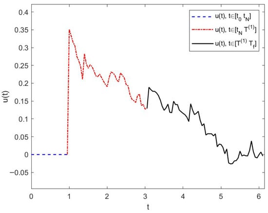
In summary, the control $u\left(t\right)$ of system (21) is designed in three stages with t in different intervals: $[t_0,t_N]$, $[t_N,T^{\left(1\right)}]$, $[T^{\left(1\right)},T_f]$. So, the control $u^{*}\left(t\right)$ has a piecewise form:

$$u^{*}\left(t\right)=\left\{\begin{array}{cc}0,\hfill & t\in [t_0,t_N],\hfill \\ -0.5066x\left(t\right)+0.2990x_r\left(t\right),\hfill & t\in [t_N,T^{\left(1\right)}],\hfill \\ -0.4267[x\left(t\right)-x_r\left(t\right)],\hfill & t\in [T^{\left(1\right)},T_f].\hfill \end{array}\right.$$

(24)

This control is the suggested hybrid $H_{\infty }$ control of (21) and (22). The trajectory of $u^{*}\left(t\right)$ with piecewise form is shown in Figure 1.

Figure 1. Trajectories of $u^{*}\left(t\right)$ in Example 1.

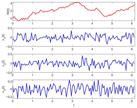
Figure 2 shows the profiles of exogenous disturbances and Brownian motion. The trajectories of $x\left(t\right)$ and $x_r\left(t\right)$ are illustrated in Figure 3, which are the solutions of (21) and (22) under the control $u\left(t\right)$ given by (24).

Figure 2. Profiles of Brownian motion and exogenous disturbance in systems (25) and (26) in Example 1.

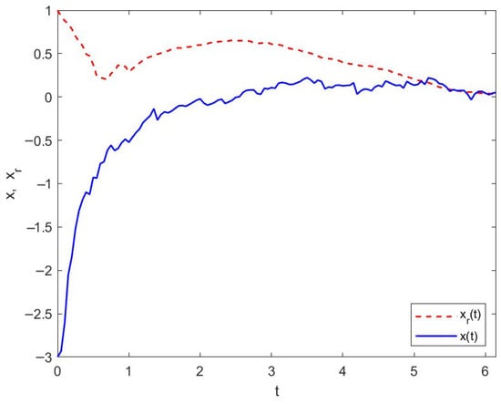
Figure 3. Trajectories of $x\left(t\right)$ and $x_r\left(t\right)$ under the control $u^{*}\left(t\right)$ in Example 1.

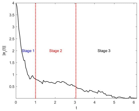
By Figure 3 and Figure 4, we see that, under the control of $u^{*}\left(t\right)$, the distance between $x\left(t\right)$ and $x_r\left(t\right)$ becomes less and the errors $e_r\left(t\right)=x\left(t\right)-x_r\left(t\right)$ also become smaller when t changes in $[t_0,T_f]$. Comparing the errors in different stages, Figure 4 illustrates that the values of errors $e_r\left(t\right)$ at the third stage ($t\in [T^{\left(1\right)},T_f]$) are smaller than in the other two stages, where $t\in [t_0,t_N]$ and $[t_N,T^{\left(1\right)}]$.

Figure 4. The changes in errors $|e_r\left(t\right)|$ under the effect of control $u^{*}\left(t\right)$ in Example 1.

Example 2. 

Consider the following 3-dimensional controlled system:

$$\begin{array}{c}\hfill \left\{\begin{array}{c}dx\left(t\right)=(Ax\left(t\right)+Bx\left(t\right)+B_1{v}_1\left(t\right))dt+(A_{1}x\left(t\right)+B_2{v}_2\left(t\right))dW\left(t\right)\hfill \\ x\left(0\right)=\left[\begin{array}{c}-3\\ 1\\ 1\end{array}\right],t\in [0,T_f]\hfill \end{array}\right.\end{array}$$

(25)

with the matrix coefficients as follows:

$$\begin{array}{c}A=\left[\begin{array}{ccc}\hfill -1.6000& \hfill 0.8000& \hfill 0\\ \hfill -0.8000& \hfill -2.0000& \hfill 1.6000\\ \hfill 0.8000& \hfill 0& \hfill -1.6000\end{array}\right], B=\left[\begin{array}{ccc}1& 0& 0\\ 0& 1& 0\\ 0& 0& 1\end{array}\right], B_1=\left[\begin{array}{c}\hfill 0.1300\\ \hfill 0.1000\\ \hfill 0.1400\end{array}\right],\hfill \\ A_1=\left[\begin{array}{ccc}\hfill -0.1280& \hfill 0.0640& \hfill 0\\ \hfill -0.0640& \hfill -0.1600& \hfill 0.1280\\ \hfill 0.0640& \hfill 0& \hfill -0.1280\end{array}\right], B_2=\left[\begin{array}{c}0.0980\\ 0.1000\\ 0.1200\end{array}\right], B_3=\left[\begin{array}{c}0.1500\\ 0.1700\\ 0.1200\end{array}\right],\hfill \\ Q=R=\left[\begin{array}{ccc}1& 0& 0\\ 0& 1& 0\\ 0& 0& 1\end{array}\right],\hfill \end{array}$$

and the reference system is also a 3-dimensional system:

$$\dot{x}\left(t\right)=A_r{x}_r\left(t\right)+B_3{v}_3,$$

(26)

where $A_r$ is an unknown matrix. Suppose the interval $[t_0,T_f]$ is divided into three segments, i.e., $[t_0,t_N]$, $[t_N,T^{\left(1\right)}]$, and $[T^{\left(1\right)},T_f]$. Now, we apply the suggested hybrid 3-stage-control method to design the $H_{\infty }$ control of (25) and (26), which includes 3 steps:

Stage 1: Observing state of $x_r\left(t\right)$ in $[t_0,t_N]$ at $t_0,t_1,t_2,\cdots ,t_N$.

In this stage, the states of reference system (26) can be observed at $t_0,t_1,t_2,\cdots ,t_N$. Suppose the observations of reference system (26) at $t_0=0,t_1=\mathrm{\Delta }t,t_2=2\mathrm{\Delta }t,\cdots ,t_N=N\mathrm{\Delta }t$ with $N=20$ are arranged as a $3\times (N+1)$ matrix denoted by $X_r=[x_{t_0},x_{t_1},\cdots ,x_{t_N}]$, whose values are observed as follows:

$$\begin{array}{c}{X}_r=\left[\begin{array}{ccccccc}2.0099& 1.9772& 1.9242& 1.8567& 1.7744& 1.6807& 1.6077\\ 3.3307& 2.8971& 2.5053& 2.1834& 1.8992& 1.6630& 1.4555\\ 1.5543& 1.5005& 1.4424& 1.4031& 1.3478& 1.2990& 1.2610\end{array}\right.\hfill \\ \hspace{1em}\hspace{1em}\hspace{1em}\begin{array}{ccccccc}1.5152& 1.4263& 1.3366& 1.2687& 1.1921& 1.1177& 1.0487\\ 1.2870& 1.1427& 1.0174& 0.9122& 0.8072& 0.7265& 0.6451\\ 1.2263& 1.1559& 1.1126& 1.0681& 1.0206& 0.9567& 0.9056\end{array}\hfill \\ \hspace{1em}\hspace{1em}\hspace{1em}\left.\begin{array}{ccccccc}0.9799& 0.8970& 0.8369& 0.7756& 0.7252& 0.6752& 0.6380\\ 0.5843& 0.5281& 0.4838& 0.4713& 0.4487& 0.4153& 0.3883\\ 0.8605& 0.8039& 0.7567& 0.7249& 0.6946& 0.6643& 0.6421\end{array}\right],\hfill \end{array}$$

where $\mathrm{\Delta }t=0.05$ is the sampling period. The inverse matrix of $X_r{X}_r^T$ is

$${\left(X_r{X}_r^T\right)}^{-1}=\left[\begin{array}{ccc}\hfill 15.6800& \hfill -2.3095& \hfill -16.5304\\ \hfill -2.3095& \hfill 0.5003& \hfill 2.2326\\ \hfill -16.5304& \hfill 2.2326& \hfill 17.7210\end{array}\right].$$

Applying the results of Theorem 1 in this stage, the estimator of $A_r$ can be obtained as follows:

$${\widehat{A}}_r=\left[\begin{array}{ccc}\hfill -2.6897& \hfill 1.0497& \hfill 0.8069\\ \hfill -2.0047& \hfill -2.8509& \hfill 3.0743\\ \hfill 0.9389& \hfill 0.1091& \hfill -2.1192\end{array}\right].$$

In this stage, there is no control input $u\left(t\right)$; i.e., $u^{1,*}\left(t\right)\equiv 0$.

Stage 2: Designing state-feedback $H_{\infty }$ control in $[t_N,T^{\left(1\right)}]$.

Taking $\rho =0.9$, by solving the Riccati inequality (17) corresponding to systems (25) and (26) with observation $X_r$, we can obtain the positive definite matrix

$$P_2=\left[\begin{array}{cccccc}\hfill 0.7505& \hfill 0.0796& \hfill 0.1836& \hfill -0.2306& \hfill -0.0259& \hfill -0.0978\\ \hfill 0.0796& \hfill 0.5933& \hfill 0.2790& \hfill 0.0234& \hfill -0.1879& \hfill -0.1338\\ \hfill 0.1836& \hfill 0.2790& \hfill 0.9542& \hfill -0.0218& \hfill -0.0622& \hfill -0.3467\\ \hfill -0.2306& \hfill 0.0234& \hfill -0.0218& \hfill 0.4721& \hfill -0.0116& \hfill 0.1373\\ \hfill -0.0259& \hfill -0.1879& \hfill -0.0622& \hfill -0.0116& \hfill 0.3991& \hfill 0.2849\\ \hfill -0.0978& \hfill -0.1338& \hfill -0.3467& \hfill 0.1373& \hfill 0.2849& \hfill 0.9738\end{array}\right].$$

Furthermore, by Theorem 2, we can get the state-feedback $H_{\infty }$ control $u^{2,*}\left(t\right)=K_2{[x^T\left(t\right),x_r^T\left(t\right)]}^T$ with

$$K_2=\left[\begin{array}{cccccc}\hfill -0.7505& \hfill -0.0796& \hfill -0.1836& \hfill 0.2306& \hfill 0.0259& \hfill 0.0978\\ \hfill -0.0796& \hfill -0.5933& \hfill -0.2790& \hfill -0.0234& \hfill 0.1879& \hfill 0.1338\\ \hfill -0.1836& \hfill -0.2790& \hfill -0.9542& \hfill 0.0218& \hfill 0.0622& \hfill 0.3467\end{array}\right].$$

Stage 3: Designing error-feedback $H_{\infty }$ control in $[T^{\left(1\right)},T_f]$.

By solving the Riccati inequality (20), the positive definite matrix $P_3$ is obtained as

$$P_3=\left[\begin{array}{cccccc}\hfill 1.4993& \hfill -0.0444& \hfill -0.0603& \hfill 0.0000& \hfill 0.0000& \hfill 0.0000\\ \hfill -0.0444& \hfill 1.5181& \hfill -0.0488& \hfill 0.0000& \hfill -0.0000& \hfill 0.0000\\ \hfill -0.0603& \hfill -0.0488& \hfill 1.4884& \hfill 0.0000& \hfill -0.0000& \hfill 0.0000\\ \hfill 0.0000& \hfill 0.0000& \hfill 0.0000& \hfill 1.4926& \hfill -0.0701& \hfill -0.0495\\ \hfill 0.0000& \hfill -0.0000& \hfill -0.0000& \hfill -0.0701& \hfill 1.4750& \hfill -0.0560\\ \hfill 0.0000& \hfill 0.0000& \hfill 0.0000& \hfill -0.0495& \hfill -0.0560& \hfill 1.5149\end{array}\right],$$

and, by results of Theorem 3, the corresponding error-feedback $H_{\infty }$ control $u^{3,*}\left(t\right)=K_3(x\left(t\right)-x_r\left(t\right))$ can be obtained, where $K_3$ is solved as

$$K_3=\left[\begin{array}{ccc}\hfill 0.0368& \hfill -0.2511& \hfill -0.0297\\ \hfill 0.2503& \hfill 0.0603& \hfill -0.2802\\ \hfill -0.0346& \hfill 0.1502& \hfill 0.0227\end{array}\right].$$

Combining the results of Stage 1, Stage 2, and Stage 3, the input control of system (25) can be rewritten as segmentation form:

$$u^{*}\left(t\right)=\left\{\begin{array}{cc}0,\hfill & t\in [t_0,t_N],\hfill \\ K_2{[x^T\left(t\right),x_r^T\left(t\right)]}^T,\hfill & t\in [t_N,T^{\left(1\right)}],\hfill \\ K_3(x\left(t\right)-x_r\left(t\right)),\hfill & t\in [T^{\left(1\right)},T_f].\hfill \end{array}\right.$$

(27)

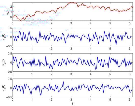
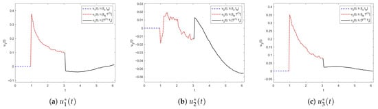
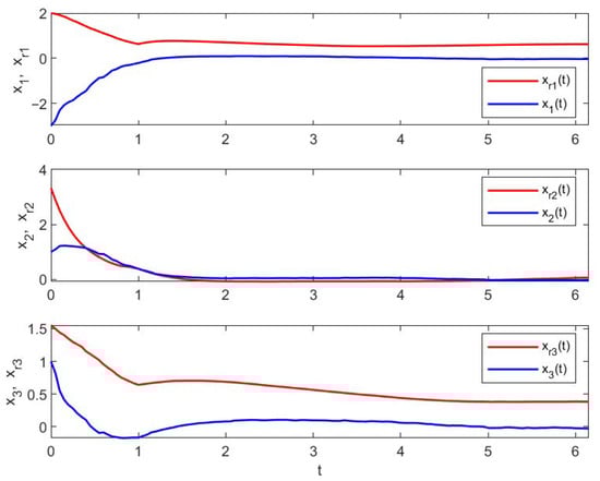
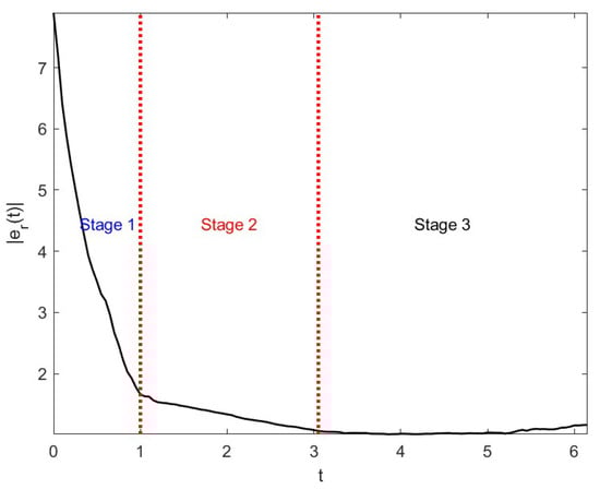
Figure 5 shows the profiles of exogenous disturbances $v_1\left(t\right)$, $v_2\left(t\right)$, $v_3\left(t\right)$, and Brownian motion $W\left(t\right)$ to which systems (25) and (26) are subjected. The trajectories of each component of the suggested $H_{\infty }$ control $u^{*}\left(t\right)$ of (25) are illustrated in Figure 6, which is divided into 3 stages. The contrast between $x\left(t\right)$ and $x_r\left(t\right)$ shown in Figure 7 and Figure 8 illustrate the change in errors between $x\left(t\right)$ and $x_r\left(t\right)$ with $|e_r\left(t\right)|=|x\left(t\right)-x_r\left(t\right)\left|\right|$. In the firs stage, i.e., $t\in [t_0,t_N]$, system (25) is no control input, where $u_1\left(t\right)=u_2\left(t\right)=u_3\left(t\right)=0$. Figure 7 and Figure 8 illustrate that the distance between $x\left(t\right)$ and $x_r\left(t\right)$ is the farthest; i.e., the values of errors $|e_r\left(t\right)|$ are worst in the first stage. In the second stage, i.e., $t\in [t_N,T^{\left(1\right)}]$, the control input of system (25) is state-feedback $H_{\infty }$ control. By Figure 7 and Figure 8, we see that, compared with the first stage, the values of errors $|e_r\left(t\right)|$ with $t\in [t_N,T^{\left(1\right)}]$ become smaller but still not very good. In the third stage, it is easy to see that the errors between $x\left(t\right)$ and $x_r\left(t\right)$ become the smallest when $t\in [T^{\left(1\right)},T_f]$, which is shown in Figure 7 and Figure 8.

Figure 5. Profiles of Brownian motion $W\left(t\right)$ and exogenous disturbance $v_1\left(t\right)$, $v_2\left(t\right)$, and $v_3\left(t\right)$ in Example 2.

Figure 6. Trajectories of $u^{*}\left(t\right)$ in Example 2.

Figure 7. Trajectories of $x\left(t\right)$ and $x_r\left(t\right)$ under the control $u^{*}\left(t\right)$ in Example 2.

Figure 8. The changes in errors $|e_r\left(t\right)|$ under the effect of control $u^{*}\left(t\right)$ in Example 2.

Example 3. 

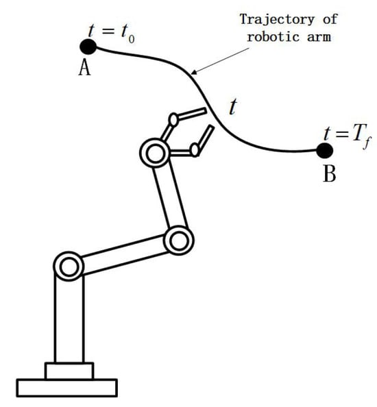
Consider the system of robot manipulator discussed in [35], whose dynamic equation is given by

$$M\left(q\right)\ddot{q}+V(q,\dot{q})+G\left(q\right)=\tau +{\tau }_d$$

(28)

where $q\left(t\right)\in {\mathbb{R}}^n$ is the vector of generalized coordinates, $M\left(q\right)\in {\mathbb{R}}^{n\times n}$ is the inertia matrix, $V(q,\dot{q})\in {\mathbb{R}}^n$ is the Coriolis and centrifugal torque vector, $G\left(q\right)\in {\mathbb{R}}^n$ is the gravitational torque vector, $\tau \in {\mathbb{R}}^n$ is the generalized control input vector, and ${\tau }_d$ is the disturbance.

See Figure 9 in order to complete the task of the robot arm moving along with a given trajectory from A to B in the time interval $[t_0,T_f]$. The control τ in (28) should be designed rationally such that $q\left(t\right)$ can take proper values at every moment $t\in [t_0,T_f]$. So, the values of $q\left(t\right)$ should track a given reference $q_d\left(t\right)$. The error between them is defined as

$$e\left(t\right)=q\left(t\right)-q_d\left(t\right).$$

Figure 9. Sketch of robot manipulator moving along the given reference trajectory.

Now, suppose $M\left(q\right)$ is an invertible positive definite constant matrix and $V(q,\dot{q})$ and $G\left(q\right)$ are linear in q and $\dot{q}$; i.e., there exist matrices $V_1,V_2,G\in {\mathbb{R}}^{n\times n}$ such that $V(q,\dot{q})=V_{1}q+V_2\dot{q}$ and $G\left(q\right)=Gq$.

Let

$$x=\left[\begin{array}{c}q\hfill \\ \dot{q}\hfill \end{array}\right],x_r=\left[\begin{array}{c}{q}_d\hfill \\ {\dot{q}}_d\hfill \end{array}\right],$$

Then, system (28) is equivalent to

$$dx\left(t\right)=[Ax\left(t\right)+B\tau \left(t\right)+B_1{\tau }_d\left(t\right)]dt.$$

Now, we extend it to the stochastic case. Denote the control $u\left(t\right)=\tau \left(t\right)$ and the exogenous disturbance $v_1\left(t\right)={\tau }_d\left(t\right)$. Suppose the stochastic system with control input has the following form:

$$dx\left(t\right)=[Ax\left(t\right)+Bu\left(t\right)+B_1{v}_1\left(t\right)]dt+[A_{1}x\left(t\right)+B_2{v}_2\left(t\right)]dW\left(t\right).$$

(29)

where

$$\begin{array}{c}A=\left[\begin{array}{cc}0& I\\ -M^{-1}(V_1+G)& -M^{-1}{V}_2\end{array}\right],B=\left[\begin{array}{c}0\\ M^{-1}\end{array}\right],\hfill \\ A_1=\left[\begin{array}{cc}0& 0\\ -M^{-1}(V_1+G)\lambda & -M^{-1}{V}_2\lambda \end{array}\right],B_1=\left[\begin{array}{c}0\\ M^{-1}\end{array}\right].\hfill \end{array}$$

In practice, system (29) is seen as a version of (28) subjected to Brownian motion $W\left(t\right)$ and exogenous disturbances $v_1\left(t\right)$ and $v_2\left(t\right)$.

We also suppose the reference trajectory $x_r\left(t\right)$ given by

$$d{x}_r\left(t\right)=[A_r{x}_r\left(t\right)+B_3{v}_3\left(t\right)]dt,$$

(30)

where $A_r\in {\mathbb{R}}^{2n\times 2n}$ is unknown, but the values of $x_r\left(t\right)$ can be observed at $t_0,t_1,\cdots ,t_N$.

Now, let $n=3$; i.e., q is a 3-dimensional vector with

$$q=\left[\begin{array}{c}{q}_1\\ q_2\\ q_3\end{array}\right],q_d=\left[\begin{array}{c}{q}_{d1}\\ q_{d2}\\ q_{d3}\end{array}\right].$$

Suppose the corresponding matrices of $M,V_1,V_2$, and G are provided as follows:

$$\begin{array}{cc}M=\left[\begin{array}{ccc}\hfill 10.2470& \hfill -1.2741& \hfill -4.7213\\ \hfill -1.2741& \hfill 14.3984& \hfill -0.3849\\ \hfill -4.7213& \hfill -0.3849& \hfill 10.5878\end{array}\right], & V_1=\left[\begin{array}{ccc}\hfill 23.4859& \hfill -0.5090& \hfill -6.4912\\ \hfill 6.3166& \hfill 29.0514& \hfill 0.3357\\ \hfill -9.8896& \hfill -6.6483& \hfill 20.1972\end{array}\right],\hfill \\ V_2=\left[\begin{array}{ccc}\hfill 36.0462& \hfill 0.1154& \hfill -11.2630\\ \hfill 15.8835& \hfill 52.9585& \hfill -17.5902\\ \hfill -13.5789& \hfill -8.6582& \hfill 34.6113\end{array}\right],& G=\left[\begin{array}{ccc}\hfill 20.6781& \hfill 0.1502& \hfill -5.5988\\ \hfill 11.2692& \hfill 29.6475& \hfill -2.1779\\ \hfill -9.9908& \hfill -6.5910& \hfill 19.7089\end{array}\right],\hfill \end{array}$$

and $\lambda =0.05$, $B_2=B_3=B$. Suppose the observations of $x_r$ at $t=t_0,t_1,\cdots ,t_N$ are obtained:

$$\begin{array}{c}\hfill X_r=\left[\begin{array}{cccccccccc}\hfill 0.2000& \hfill 0.2250& \hfill 0.2417& \hfill 0.2514& \hfill 0.2556& \hfill 0.2552& \hfill 0.2512& \hfill 0.2444& \hfill 0.2355& \hfill 0.2250\\ \hfill -0.2200& \hfill -0.2450& \hfill -0.2656& \hfill -0.2825& \hfill -0.2961& \hfill -0.3068& \hfill -0.3151& \hfill -0.3212& \hfill -0.3253& \hfill -0.3276\\ \hfill 0.7000& \hfill 0.7050& \hfill 0.6999& \hfill 0.6865& \hfill 0.6666& \hfill 0.6415& \hfill 0.6126& \hfill 0.5808& \hfill 0.5471& \hfill 0.5122\\ \hfill 0.5000& \hfill 0.3330& \hfill 0.1953& \hfill 0.0829& \hfill -0.0078& \hfill -0.0797& \hfill -0.1358& \hfill -0.1784& \hfill -0.2097& \hfill -0.2315\\ \hfill -0.5000& \hfill -0.4126& \hfill -0.3373& \hfill -0.2719& \hfill -0.2150& \hfill -0.1651& \hfill -0.1211& \hfill -0.0822& \hfill -0.0476& \hfill -0.0167\\ \hfill 0.1000& \hfill -0.1029& \hfill -0.2674& \hfill -0.3985& \hfill -0.5010& \hfill -0.5788& \hfill -0.6356& \hfill -0.6745& \hfill -0.6984& \hfill -0.7095\end{array}\right.\\ \hfill \begin{array}{cccccccccc}\hfill 0.2134& \hfill 0.2011& \hfill 0.1885& \hfill 0.1757& \hfill 0.1630& \hfill 0.1506& \hfill 0.1386& \hfill 0.1270& \hfill 0.1160& \hfill 0.1056\\ \hfill -0.3285& \hfill -0.3279& \hfill -0.3262& \hfill -0.3233& \hfill -0.3194& \hfill -0.3147& \hfill -0.3091& \hfill -0.3029& \hfill -0.2960& \hfill -0.2886\\ \hfill 0.4767& \hfill 0.4412& \hfill 0.4061& \hfill 0.3717& \hfill 0.3384& \hfill 0.3063& \hfill 0.2756& \hfill 0.2465& \hfill 0.2190& \hfill 0.1932\\ \hfill -0.2456& \hfill -0.2531& \hfill -0.2554& \hfill -0.2535& \hfill -0.2484& \hfill -0.2407& \hfill -0.2311& \hfill -0.2201& \hfill -0.2082& \hfill -0.1958\\ \hfill 0.0108& \hfill 0.0355& \hfill 0.0576& \hfill 0.0775& \hfill 0.0951& \hfill 0.1109& \hfill 0.1249& \hfill 0.1373& \hfill 0.1481& \hfill 0.1575\\ \hfill -0.7102& \hfill -0.7023& \hfill -0.6872& \hfill -0.6666& \hfill -0.6415& \hfill -0.6131& \hfill -0.5823& \hfill -0.5497& \hfill -0.5161& \hfill -0.4821\end{array}\\ \hfill \left.\begin{array}{ccccccccccc}\hfill 0.0958& \hfill 0.0867& \hfill 0.0781& \hfill 0.0702& \hfill 0.0630& \hfill 0.0563& \hfill 0.0501& \hfill 0.0445& \hfill 0.0394& \hfill 0.0348& \hfill 0.0306\\ \hfill -0.2807& \hfill -0.2724& \hfill -0.2638& \hfill -0.2549& \hfill -0.2458& \hfill -0.2365& \hfill -0.2271& \hfill -0.2176& \hfill -0.2081& \hfill -0.1986& \hfill -0.1892\\ \hfill 0.1691& \hfill 0.1467& \hfill 0.1260& \hfill 0.1069& \hfill 0.0895& \hfill 0.0736& \hfill 0.0592& \hfill 0.0462& \hfill 0.0345& \hfill 0.0242& \hfill 0.0150\\ \hfill -0.1831& \hfill -0.1704& \hfill -0.1579& \hfill -0.1457& \hfill -0.1339& \hfill -0.1226& \hfill -0.1119& \hfill -0.1019& \hfill -0.0925& \hfill -0.0837& \hfill -0.0756\\ \hfill 0.1655& \hfill 0.1723& \hfill 0.1779& \hfill 0.1823& \hfill 0.1857& \hfill 0.1881& \hfill 0.1896& \hfill 0.1903& \hfill 0.1901& \hfill 0.1892& \hfill 0.1876\\ \hfill -0.4480& \hfill -0.4143& \hfill -0.3812& \hfill -0.3491& \hfill -0.3180& \hfill -0.2882& \hfill -0.2599& \hfill -0.2330& \hfill -0.2076& \hfill -0.1838& \hfill -0.1615\end{array}\right].\end{array}$$

where $t_0=0,t_k=k\mathrm{\Delta }t,k=1,2,\cdots ,30$ with $\mathrm{\Delta }t=0.05$. By Theorem 1, we can obtain the estimator of $A_r$:

$${\widehat{A}}_r=\left[\begin{array}{cccccc}\hfill -1.8585& \hfill 0.2796& \hfill 0.9931& \hfill 0.9700& \hfill 0.4932& \hfill -0.0032\\ \hfill 1.6188& \hfill -0.1667& \hfill -0.8638& \hfill 0.1287& \hfill 0.6264& \hfill -0.0664\\ \hfill 0.8675& \hfill -0.1626& \hfill -0.4663& \hfill -0.0249& \hfill -0.2543& \hfill 1.0276\\ \hfill -2.8913& \hfill -0.1483& \hfill -1.6393& \hfill -3.8331& \hfill -0.6145& \hfill -0.3722\\ \hfill -0.4257& \hfill -4.2336& \hfill -0.7023& \hfill -1.4485& \hfill -4.0145& \hfill 1.1032\\ \hfill -0.5798& \hfill 1.0479& \hfill -3.9362& \hfill -0.6826& \hfill 0.5743& \hfill -3.2811\end{array}\right].$$

Construct the augmented system of (29) and (30) with ${\widehat{A}}_r$ given above. Then, for $\rho =0.8$, applying the results of Theorems 2 and 3, the state-feedback $H_{\infty }$ control and error-feedback $H_{\infty }$ control are designed, which are given as follows:

$${\tau }^{*}\left(t\right)=u^{*}\left(t\right)=\left\{\begin{array}{cc}0,\hfill & t\in [t_0,t_N],\hfill \\ K_2{[x^T\left(t\right),x_r^T\left(t\right)]}^T,\hfill & t\in [t_N,T^{\left(1\right)}],\hfill \\ K_3(x\left(t\right)-x_r\left(t\right)),\hfill & t\in [T^{\left(1\right)},T_f].\hfill \end{array}\right.$$

(31)

where

$$K_2=\left[\begin{array}{cccccccccccc}\hfill -0.0266& \hfill -0.0039& \hfill -0.0122& \hfill -0.0397& \hfill 0.0029& \hfill -0.0141& \hfill 0.0056& \hfill 0.0000& \hfill 0.0096& \hfill 0.0141& \hfill -0.0010& \hfill 0.0081\\ \hfill 0.0021& \hfill -0.0192& \hfill 0.0007& \hfill 0.0038& \hfill -0.0262& \hfill -0.0099& \hfill 0.0076& \hfill 0.0101& \hfill -0.0050& \hfill 0.0015& \hfill 0.0103& \hfill 0.0021\\ \hfill -0.0092& \hfill -0.0121& \hfill -0.0277& \hfill -0.0097& \hfill -0.0098& \hfill -0.0456& \hfill 0.0097& \hfill 0.0056& \hfill 0.0103& \hfill 0.0053& \hfill 0.0031& \hfill 0.0188\end{array}\right]$$

and

$$K_3=\left[\begin{array}{cccccc}\hfill 1.0647& \hfill 0.0374& \hfill -0.3934& \hfill -1.3155& \hfill 0.2722& \hfill 0.6980\\ \hfill -0.1236& \hfill 1.2073& \hfill 0.3950& \hfill 0.3407& \hfill -1.6582& \hfill -0.2415\\ \hfill -0.5678& \hfill -0.3900& \hfill 0.9147& \hfill 0.6441& \hfill -0.1463& \hfill -1.4583\end{array}\right]$$

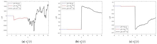
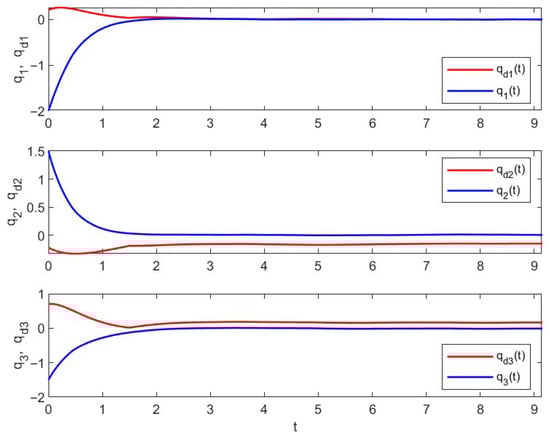
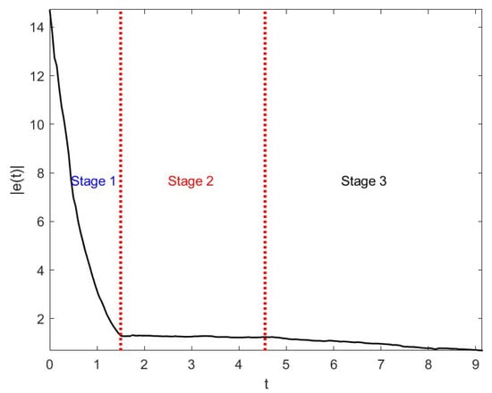
Figure 10 illustrates the trajectories of control ${\tau }^{*}\left(t\right)$ with three stages. Figure 11 shows the trajectories of $q\left(t\right)$ and reference $q_d\left(t\right)$ under the control ${\tau }^{*}\left(t\right)$ designed above. It is easy to see that each component of $q\left(t\right)$ performs well regarding the reference $q_d\left(t\right)$. Figure 12 illustrates the error’s changes between $q\left(t\right)$ and $q_d\left(t\right)$, showing that there exists the smallest error in the third stage, which verifies the effect of the proposed method.

Figure 10. Trajectories of $u^{*}\left(t\right)$ in Example 3.

Figure 11. Trajectories of $x\left(t\right)$ and $x_r\left(t\right)$ under the control $u^{*}\left(t\right)$ in Example 3.

Figure 12. The changes in errors $|e_r\left(t\right)|$ under the effect of control $u^{*}\left(t\right)$ in Example 3.

6. Conclusions

The robust $H_{\infty }$ tracking problem is investigated for linear stochastic systems where the parameters of a reference system are unknown but some discrete-time observations are available. A hybrid data-driven $H_{\infty }$ tracking-control design scheme is proposed for such problems. By using the least-squares method, the parameters of the reference system are estimated and the corresponding data-dependent augmented systems are established. Based on the solutions of algebraic Riccati inequalities, the state-feedback and error-feedback $H_{\infty }$ controls are designed for such tracking problems to enhance system performance and reduce tracking error. Moreover, the programming evolution of the hybrid control method is summarized, which includes data observation, state-feedback $H_{\infty }$ control, and error-feedback $H_{\infty }$ control.

References

- Persis, C.D.; Tesi, P. Formulas for data-driven control: Stabilization, optimality, and robustness. IEEE Trans. Autom. Control 2020, 65, 909–924. [Google Scholar] [CrossRef]
- Shen, D.; Zhang, W.; Wang, Y.; Chien, C. On almost sure and mean square convergence of P-type ILC under randomly varying iteration lengths. Automatica 2016, 63, 359–365. [Google Scholar] [CrossRef]
- Yu, H.; Guan, Z.; Chen, T.; Yamamoto, T. Design of data-driven PID controllers with adaptive updating rules. Automatica 2020, 121, 109185. [Google Scholar] [CrossRef]
- Hou, Z.; Xiong, S. On model-free adaptive control and its stability analysis. IEEE Trans. Autom. Control 2019, 64, 4555–4569. [Google Scholar] [CrossRef]
- Pang, Z.; Ma, B.; Liu, G.; Han, Q. Data-driven adaptive control: An incremental triangular dynamic linearization approach. IEEE Trans. Circuits Syst. II Express Briefs 2022, 69, 4949–4953. [Google Scholar] [CrossRef]
- Wang, Z.; Liu, K.; Cheng, X.; Sun, X. Online data-driven model predictive control for switched linear systems. IEEE Trans. Autom. Control 2025, 70, 6222–6229. [Google Scholar] [CrossRef]
- Wu, W.; Qiu, L.; Rodriguez, J.; Liu, X.; Ma, J.; Fang, Y. Data-driven finite control-set model predictive control for modular multilevel converter. IEEE J. Emerg. Sel. Top. Power Electron. 2023, 11, 523–531. [Google Scholar] [CrossRef]
- Sun, T.; Sun, X.; Sun, A. Optimal output tracking of aircraft engine systems: A data-driven adaptive performance seeking control. IEEE Trans. Circuits Syst. II Express Briefs 2022, 69, 1467–1471. [Google Scholar] [CrossRef]
- Liu, W.; Sun, J.; Wang, G.; Bullo, F.; Chen, J. Data-driven self-triggered control via trajectory prediction. IEEE Trans. Autom. Control 2023, 68, 6951–6958. [Google Scholar] [CrossRef]
- Zhan, J.; Ma, Z.; Zhang, L. Data-driven modeling and distributed predictive control of mixed vehicle platoons. IEEE Trans. Intell. Veh. 2023, 8, 572–582. [Google Scholar] [CrossRef]
- Zhang, W.; Xie, L.; Chen, B.S. Stochastic H2/H∞ Control: A Nash Game Approach; Taylor & Francis: Boca Raton, FL, USA, 2017. [Google Scholar]
- Chen, B.S.; Wang, C.P.; Lee, M.Y. Stochastic robust team tracking control of multi-UAV networked system under Wiener and Poisson random fluctuations. IEEE Trans. Cybern. 2021, 51, 5786–5799. [Google Scholar] [CrossRef] [PubMed]
- Liu, H.; Ma, T.; Lewis, F.L.; Wan, Y. Robust formation control for multiple quadrotors with nonlinearities and disturbances. IEEE Trans. Cybern. 2020, 50, 1362–1371. [Google Scholar] [CrossRef]
- Zhao, J.; Zhao, H.; Song, Y.; Sun, Z.Y.; Yu, D. Fast finite-time consensus protocol for high-order nonlinear multi-agent systems based on event-triggered communication scheme. Appl. Math. Comput. 2026, 508, 129631. [Google Scholar] [CrossRef]
- Boshkovska, E.; Ng, D.W.K.; Zlatanov, N.; Koelpin, A.; Schober, R. Robust resource allocation for MIMO wireless powered communication networks based on a non-linear EH model. IEEE Trans. Commun. 2017, 65, 1984–1999. [Google Scholar] [CrossRef]
- Zames, G. Feedback and optimal sensitivity: Model reference transformations, multiplicative seminorms, and approximate inverses. IEEE Trans. Autom. Control 1981, 26, 301–320. [Google Scholar] [CrossRef]
- Doyle, J.C.; Glover, K.; Khargonekar, P.; Francis, B. State-space solutions to standard H2 and H∞ control problems. IEEE Trans. Autom. Control 1989, 34, 831–847. [Google Scholar] [CrossRef]
- Gahinet, P.; Apkarian, P. A linear matrix inequality approach to H∞ control. Int. J. Robust Nonlinear Control 1994, 4, 21–448. [Google Scholar] [CrossRef]
- Dai, X.; Zuo, H.; Deng, F. Mean square finite-time stability and stabilization of impulsive stochastic distributed parameter systems. IEEE Trans. Syst. Man Cybern. Syst. 2025, 55, 4064–4075. [Google Scholar] [CrossRef]
- Zhao, J.; Yuan, Y.; Sun, Z.Y.; Xie, X. Applications to the dynamics of the suspension system of fast finite time stability in probability of p-norm stochastic nonlinear systems. Appl. Math. Comput. 2023, 457, 128221. [Google Scholar] [CrossRef]
- Hinrichsen, D.; Pritchard, A.J. Stochastic H∞. SIAM J. Control Optim. 1998, 36, 1504–1538. [Google Scholar] [CrossRef]
- der Schaft, A.J.V. On a state-space approach to nonlinear H∞ control. Syst. Control Lett. 1991, 16, 1–8. [Google Scholar]
- Ball, J.A.; Helton, J.W.; Walker, M.L. H∞ control for nonlinear systems with output feedback. IEEE Trans. Autom. Control 1993, 38, 546–559. [Google Scholar] [CrossRef]
- Zhang, W.; Chen, B.S. State feedback H∞ control for a class of nonlinear stochastic systems. SIAM J. Control Optim. 2006, 44, 1973–1991. [Google Scholar] [CrossRef]
- Lin, X.; Zhang, T.; Zhang, W.; Chen, B.S. New approach to general nonlinear discrete-Time stochastic H∞ control. IEEE Trans. Autom. Control 2019, 64, 1472–1486. [Google Scholar] [CrossRef]
- Chen, B.S.; Yang, C.T.; Lee, M.Y. Multiplayer noncooperative and cooperative minimax H∞ tracking game strategies for linear mean-field stochastic systems with applications to cyber-social systems. IEEE Trans. Cybern. 2022, 52, 2968–2980. [Google Scholar]
- Xin, Y.; Zhang, W.; Wang, D.; Zhang, T.; Jiang, X. Stochastic H2/H∞ control for discrete-time multi-agent systems with state and disturbance-dependent noises. Int. J. Robust Nonlinear Control 2025, preprinted. [Google Scholar] [CrossRef]
- Zhao, J.; Wang, Z.; Lv, Y.; Na, J.; Liu, C.; Zhao, Z. Data-driven learning for H∞ control of adaptive cruise control systems. IEEE Trans. Veh. Technol. 2024, 73, 18348–18362. [Google Scholar] [CrossRef]
- Liao, Y.; Zhang, T.; Yan, X.; Jiang, D. Integrated guidance and tracking control for underactuated AUVs on SE(3) with singularity-free global prescribed performance attitude control. Ocean Eng. 2025, 342, 122770. [Google Scholar] [CrossRef]
- Zhang, L.; Sun, Y.; Chai, P.; Tan, J.; Zheng, H. Prescribed-performance time-delay compensation control for UUV trajectory tracking in main-branch water conveyance tunnel transitions under unknown input delays. Ocean Eng. 2025, 342, 122941. [Google Scholar]
- Xu, B.; Dai, Y.; Suleman, A.; Shi, Y. Distributed fault-tolerant control of multi-UAV formation for dynamic leader tracking: A Lyapunov-based MPC framework. Automatica 2025, 175, 112179. [Google Scholar] [CrossRef]
- Luque, I.; Chanfreut, P.; Limón, D.; Maestre, J.M. Model predictive control for tracking with implicit invariant sets. Automatica 2025, 179, 112436. [Google Scholar] [CrossRef]
- Chen, B.S.; Hsueh, C.H.; Wu, R.S. Optimal H∞ adaptive fuzzy observer-based reference tracking control of nonlinear stochastic systems under uncertain measurement function and noise. Fuzzy Sets Syst. 2025, 521, 109597. [Google Scholar] [CrossRef]
- Lin, X.; Zhang, R. H∞ Control for stochastic systems with Poisson jumps. J. Syst. Sci. Complex 2011, 24, 683–700. [Google Scholar] [CrossRef]
- Song, G.; Park, H.; Kim, J. The H∞ Robust stability and performance conditions for uncertain robot manipulators. IEEE/CAA Hournal Autom. Sin. 2025, 12, 270–272. [Google Scholar] [CrossRef]
Disclaimer/Publisher’s Note: The statements, opinions and data contained in all publications are solely those of the individual author(s) and contributor(s) and not of MDPI and/or the editor(s). MDPI and/or the editor(s) disclaim responsibility for any injury to people or property resulting from any ideas, methods, instructions or products referred to in the content. |
© 2025 by the authors. Licensee MDPI, Basel, Switzerland. This article is an open access article distributed under the terms and conditions of the Creative Commons Attribution (CC BY) license (https://creativecommons.org/licenses/by/4.0/).