Abstract
Citrus Huanglongbing (HLB) is one of the most destructive diseases in the global citrus industry; its pathogen is transmitted primarily by the Asian citrus psyllid (ACP), Diaphorina citri Kuwayama, making timely monitoring and control of ACP populations essential. Real-world ACP monitoring faces several challenges, including tiny targets easily confused with the background, noise amplification and spurious detections caused by textures, stains, and specular glare on yellow-boards, unstable localization due to minute shifts of small boxes, and strict constraints on parameters, computation, and model size for long-term edge deployment. To address these challenges, we focus on the yellow-board ACP monitoring scenario and create the ACP Yellow Sticky Trap Dataset (ACP-YSTD), which standardizes background and acquisition procedures, covering common interference sources. The dataset consists of 600 images with 3837 annotated ACP, serving as a unified basis for training and evaluation. On the modeling side, we propose TGSP-YOLO11, an improved YOLO11-based detector: the detection head is reconfigured to the two scales P2 + P3 to match tiny targets and reduce redundant paths; Guided Scalar Fusion (GSF) is introduced on the high-resolution branch to perform constrained, lightweight scalar fusion that suppresses noise amplification; ShapeIoU is adopted for bounding-box regression to enhance shape characterization and alignment robustness for small objects; and Network Slimming is employed for channel-level structured pruning, markedly reducing parameters, FLOPs, and model size to satisfy edge deployment, without degrading detection performance. Experiments show that on the ACP-YSTD test set, TGSP-YOLO11 achieves precision 92.4%, recall 95.5%, and F1 93.9, with 392,591 parameters, a model size of 1.4 MB, and 6.0 GFLOPs; relative to YOLO11n, recall increases by 4.6%, F1 by 2.4, and precision by 0.2%, while the parameter count, model size, and computation decrease by 84.8%, 74.5%, and 4.8%, respectively. Compared to representative detectors (SSD, RT-DETR, YOLOv7-tiny, YOLOv8n, YOLOv9-tiny, YOLOv10n, YOLOv12n, YOLOv13n), TGSP-YOLO11 improves recall by 33.9%, 19.0%, 8.5%, 10.1%, 6.3%, 4.6%, 6.9%, and 5.7%, respectively, and F1 by 19.9, 14.9, 5.1, 6.0, 2.6, 5.6, 3.6, and 3.9, respectively. Additionally, it reduces parameter count, model size, and computation by 84.0–98.8%, 74.5–97.9%, and 3.2–94.2%, respectively. Transfer evaluation indicates that on 20 independent yellow-board images not seen during training, the model attains precision 94.3%, recall 95.8%, F1 95.0, and 159.2 FPS.
MSC:
68T07
1. Introduction
Citrus Huanglongbing (HLB) is recognized as one of the most destructive diseases threatening the global citrus industry []. Its pathogen is a phloem-limited bacterium of the genus Candidatus Liberibacter, and transmission relies mainly on the Asian citrus psyllid (ACP), Diaphorina citri Kuwayama [,]. Infected trees often show stunted growth, leaf chlorosis, and reduced fruit quality, with severe cases leading to tree death, posing risks to sustainable production and economic returns [,]. In practice, ACP monitoring has long depended on manual patrols. ACPs are very small, highly mobile, and elusive [,], so manual searching and imaging are time-consuming and inefficient. Manual methods also fail to provide continuous, wide-area, spatiotemporally consistent monitoring data, which limits precise control. Therefore, there is an urgent need for an automated monitoring solution that is sustainable and scalable. Compared to earlier handcrafted-feature-based methods, deep learning object detection learns discriminative representations end-to-end and has demonstrated significant advantages in agricultural pest and disease recognition [,,]. Representative frameworks include the two-stage Faster Region-based Convolutional Neural Networks (Faster R-CNN) [] and the single-stage You Only Look Once (YOLO) [] and Single Shot MultiBox Detector (SSD) [].
Most existing studies focus on ACP detection in natural scenes. Lyu et al. [] achieved good generalization in orchards based on YOLOv5s-BC. Dai et al. [] combined an improved Cascade R-CNN with a high-definition field imaging system and verified applicability to ACP and other small targets (e.g., fruit flies). Wang et al. [] proposed improvements to YOLOX and further enhanced detection performance. Overall, these studies show that, under complex backgrounds and scale variations, deep learning frameworks outperform traditional methods.
However, natural-scene solutions usually rely on manual framing and close-range imaging, which makes it difficult to achieve large-scale, long-term, and near-real-time monitoring. At the same time, ACPs are tiny and easily occluded, which increases the risk of missed detections and raises labor costs. These constraints create a bottleneck for large-scale applications based solely on natural-scene recognition. Given these limitations, recent research has shifted to a “capture-first, recognize-later” route: deploying yellow sticky board (hereafter “yellow-board”) that leverages ACPs’ sensitivity to yellow. This provides a fixed acquisition carrier and a uniform, low-interference background, reduces detection difficulty at the source, and lays a foundation for standardized and scalable monitoring systems.
For ACP detection on yellow-board, existing work has verified the feasibility and effectiveness of this route. Da Cunha et al. [] developed the ACP detector, a web application based on image processing and deep learning, and reported precision, recall, and F1 scores of 90.0%, 70.0%, and 79.0 using the original YOLOv7. Li et al. [] proposed YOLOv8-MC and built a remote monitoring system; the improved model achieved precision, recall, and F1 of 90.6%, 91.2%, and 91.0. These results suggest that a uniform background improves target contrast and reduces background interference, leading to more stable detection. However, issues such as insect adhesion, occlusion, and glare on the glue surface persist, requiring improved small-target separation and fine-grained representation.
In summary, the yellow-board route effectively reduces scene interference through a uniform background and fixed carrier, and it has shown progress in practice. Yet reliable and large-scale application still faces three challenges. First, targets are extremely small and often accompanied by adhesion, overlap, and glare; insufficient fine-detail representation tends to cause both missed and false detections. Second, high-frequency interference from board textures and stains may be amplified in high-resolution features and affect the confidence distribution, while bounding-box regression is sensitive to slight deformations, which weakens recall and localization stability. Third, long-term edge deployment imposes strict constraints on parameter count, computation, and model size; existing methods still have room for compression and system-level evaluation. Therefore, systematic optimization is required around scale matching, robust fusion, shape-sensitive regression, and structured compression.
Building on yellow-board ACP studies and recent YOLOv12 and YOLOv13 advances, this work synthesizes four axes—detector head level/configuration, feature-fusion strategy (neck), box regression loss, and deployment costs—as summarized in Table 1. Existing yellow-board methods typically adopt P3 + P4 + P5 heads with Path Aggregation Network and Feature Pyramid Network fusion, yet explicit P2-level modeling for ultra-small objects and noise constraints on high-resolution branches are under-addressed. While YOLOv12/v13 strengthen global dependencies via attention and cross-scale correlation, their default heads remain centered on P3 + P4 + P5. Consequently, an effective path for yellow-boards should balance lower-level heads (P2), constrained fusion on high-resolution branches, and shape-aligned small-box regression, which motivates the methodology that follows.

Table 1.
Comparative technical roadmaps for yellow-board Asian citrus psyllid (ACP) detection and recent YOLOv12 and YOLOv13 models. N/R = not reported.
To address these problems, this study proposes a yellow-board ACP recognition method based on an improved YOLO11 (denoted TGSP-YOLO11), with two main components:
- We construct the ACP Yellow Sticky Trap Dataset (ACP-YSTD) to standardize the background and acquisition process, cover real interference factors on yellow-board, and provide a standardized data basis for model training and testing.
- We propose the improved model TGSP-YOLO11: for scale mismatch on tiny targets, we reconstruct the detection head to two scales (P2 + P3) to better match target size, enhance spatial detail utilization, and reduce redundant paths; to suppress noise amplification in the high-resolution branch, we introduce Guided Scalar Fusion (GSF) to perform constrained, lightweight scalar fusion, thereby reducing false positives; to improve shape characterization and alignment robustness for tiny boxes, we replace CIoU [] with ShapeIoU [] and introduce a direction-aware shape measure to enhance contour alignment and localization stability; to meet edge-side resource constraints, we adopt Network Slimming [] for channel-level structured pruning, which significantly reduces parameters, FLOPs, and model size.
These data and model components support each other to improve small-target detection performance and strengthen edge deployability.
2. Materials and Methods
2.1. Data Collection and Annotation
ACPs in natural environments are shown in Figure 1. Adults are about 3 mm long. Their bodies are grayish green with brownish markings and covered with white wax. The targets are small and easily confused with the background. The data in this study were collected at an experimental plantation for citrus HLB in Haizhu District, Guangzhou, Guangdong Province, during June–August 2025. Yellow-boards (15 × 10 cm) were randomly hung within the orchard, with positions not limited to the canopy; different tree positions and heights were covered to enhance scene diversity. Each board was hung for 3–10 days per session. Multi-batch deployment and recovery were used to cover different time periods and environmental changes, enhancing the spatiotemporal representativeness of the samples. To obtain stable and clear images, the recovered boards were transported to the laboratory for imaging, reducing the impact of strong outdoor glare and shadows on image quality.
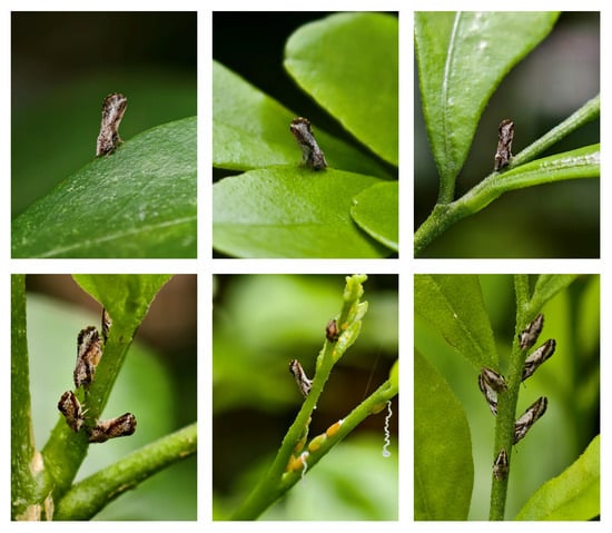
Figure 1.
ACP in natural environments (illustrative field photos; not used for ACP Yellow Sticky Trap Dataset (ACP-YSTD) training or evaluation). Adults are about 3 mm in length; typical backgrounds/poses are shown.
A high-definition macro-imaging protocol was used. The working distance between the camera and the board was kept within 28–35 cm. The resolution of a single image was 3072 × 4080 pixels. Fixed fill lights were used in the laboratory to provide consistent illumination against a uniform background. Basic quality control was performed, and images with obvious defocus or severe glare were removed. In total, 600 high-definition yellow-board images were obtained to form the ACP-YSTD. On this basis, high-quality manual annotation was performed and strictly reviewed according to unified guidelines. An annotation example is shown in Figure 2. Finally, 3837 annotated instances of ACP were obtained, providing reliable data support for subsequent model training and evaluation.
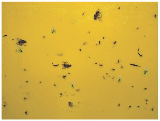
Figure 2.
ACP annotations on yellow-board from the ACP-YSTD dataset. Bounding boxes denote the ACP class on laboratory-captured yellow-board images.
To illustrate confounding factors and target diversity, Figure 3 shows representative morphologies of ACP and look-alike insects. Rows 1 and 2 present typical ACP samples, whereas Rows 3 and 4 show other insect samples.
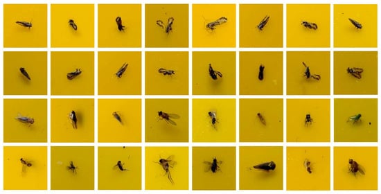
Figure 3.
Representative morphologies of ACP and look-alike insects in ACP-YSTD (Rows 1–2: ACP; Rows 3–4: other insects).
2.2. Dataset Preparation
In yellow-board images, targets are often dense and very small. A common practice is to crop the full image into fixed-size patches to enlarge the target scale, but this introduces two notable problems. First, cropping may split the same insect into different patches. If training/validation/test sets are divided by patches, implicit cross-subset data leakage can occur. Second, during inference, a sliding-window covering strategy is required to traverse the entire board region. This significantly increases computation and deployment complexity and is unfavorable for long-term stable operation on edge devices. In addition, if the common YOLO input resolution of 640 × 640 is used directly, the original 3072 × 4080 images are excessively downsampled. The edges and textures of small targets decay markedly, which affects the discrimination of tiny instances such as ACP.
To address these trade-offs, the model input size was set to 960 × 960, ensuring consistency between training and inference. Compared with 640 × 640, 960 × 960 provides a higher effective pixel density for ACP of about 3 mm without changing the sample granularity, reducing information loss of small targets during scaling. At the same time, no cropping was performed, which avoids the same instance appearing across samples and the resulting risk of potential data leakage. During inference, the entire yellow-board image can be detected in one pass without extra tiling or sliding windows. This simplifies the deployment pipeline, reduces latency variability and engineering complexity, and better fits long-term online monitoring on edge devices. Overall, a unified 960 × 960 input achieves a more balanced trade-off between detection accuracy demands and computational budget, helping ensure the resolvability of small targets while maintaining stability and efficiency in training and inference.
3. Experimental Methods
3.1. TGSP-YOLO11
In this study, after multi-faceted considerations and extensive baseline comparisons, we adopt YOLO11 as the base model. Specifically, unless otherwise stated, our baseline is the official Ultralytics YOLO11n (nano) release; we follow the default architecture and training settings from the standard open-source Ultralytics YOLO11 implementation. YOLO11 offers a favorable speed–accuracy trade-off, a stable training–inference pipeline, and mature operator-level and engineering support [,,]. These properties make it suitable for targeted structural modification and lightweight deployment in a “single-class, tiny-target, edge-deployment” scenario of ACP on yellow-board. However, directly using the original architecture faces four key challenges: (1) the conventional P3 + P4 + P5 three-branch prediction causes resolution mismatch and redundant computation for very small targets; (2) the high-resolution branch is easily disturbed by yellow-board textures, stains, and other artifacts, and simple linear fusion can amplify noise and increase false positives; (3) CIoU does not sufficiently capture shape inconsistency or minor alignment errors on tiny boxes, which limits localization stability; and (4) for large-scale edge deployment, the original model still requires further compression in parameters, model size, and computation to reduce cost and ensure long-term reliable operation.
To address these issues, we propose TGSP-YOLO11. First, we perform a two-scale feature reconfiguration for tiny targets, focusing only on P2 and P3 to match target size, reduce redundant paths, and improve separability from the background. Second, we introduce GSF to achieve constrained, lightweight scalar fusion on the high-resolution branch, preserving fine details while suppressing the adverse impact of noise on the confidence distribution. Third, we replace CIoU with ShapeIoU, which introduces a direction-aware shape measure to improve contour alignment and localization stability on tiny targets. Finally, we adopt Network Slimming for structured pruning, which significantly reduces parameters, model size, and FLOPs while maintaining detection performance.
In summary, TGSP-YOLO11 combines P2 + P3 reconfiguration, GSF-based noise-suppressed fusion, ShapeIoU-based shape-sensitive regression, and Network-Slimming-based structured compression. It improves recall for tiny targets while maintaining accuracy and greatly lowering model cost, meeting the edge-deployment requirements of yellow-board scenarios. The overall framework of TGSP-YOLO11 is shown in Figure 4.
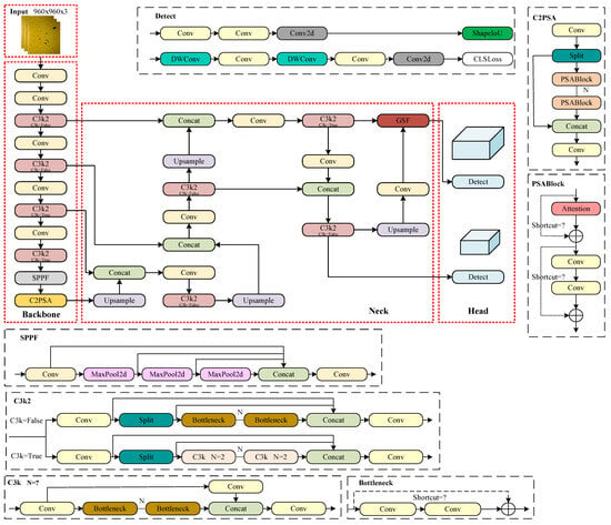
Figure 4.
Overall structure of TGSP-YOLO11.
3.1.1. Two-Scale Feature Reconfiguration for Tiny Targets
On ACP-YSTD, under an input size of , ACP targets are predominantly tiny: the average width and height are about 20 pixels; the minimum width is about 6.6 pixels, the maximum width about 37.9 pixels; the minimum height about 8.1 pixels, and the maximum height about 39.8 pixels (see Table 2). Under such tiny-target settings, the conventional multi-scale strategy that predicts simultaneously on P3, P4, and P5 is not well matched: higher layers provide stronger semantics but much lower spatial resolution, which makes it difficult to preserve the boundaries and fine details of tiny instances. In addition, extra high-level detection branches and aggregation paths introduce computation and memory overhead that is unfavorable for lightweight deployment at the edge.

Table 2.
Target size statistics on ACP-YSTD at input px (computed over the full dataset).
From a sampling perspective, P2/P3 have strides of 4/8 relative to the input, so an average 20-px box spans about 5 and about 2.5 sampling units on P2 and P3, respectively; even the minimum boxes (about 6.6–8.1 px) correspond to roughly 1.7–2.0 units on P2. By contrast, P4/P5 (strides 16/32) over-quantize tiny boxes (averaging about 1.2 and 0.6 units; minima below 1), which degrades recall and localization stability due to insufficient spatial support.
Based on this analysis, we reconfigure the YOLO11 neck and head to focus detection on two higher-resolution scales, P2 and P3. In the top-down fusion path, P4 is retained only as an intermediate enhancement level, while final detections are produced on P2 and P3; the P5 branch and its routes to the head are omitted. A lightweight bottom-up feedback path then refines P3 with fine-grained information, improving feature expression for tiny targets. This design aligns spatial resolution with target size, reduces redundant high-level branches and complex aggregation, and concentrates capacity on the most useful scales, thereby balancing accuracy and efficiency and making the model more suitable for edge deployment.
3.1.2. Guided Scalar Fusion
After extending the detection head from the conventional P3 + P4 + P5 to P2 + P3, the high-resolution branch better covers tiny targets of about 6–40 pixels, thereby improving recall; however, P2 also carries more high-frequency noise from yellow-board textures, stains, and other insects. If features are directly summed or combined with unconstrained linear weights, the noisy branch can be indiscriminately amplified, shifting the confidence distribution and increasing false positives. To preserve P2 fine details while suppressing noise amplification, we introduce a parameter-lightweight GSF module between the neck and the head. GSF achieves robust fusion via nonnegative, -stabilized normalized weights and a small main-branch residual. The architecture of GSF is shown in Figure 5.
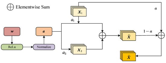
Figure 5.
Structure of the Guided Scalar Fusion (GSF) module. Two inputs (P2 and upsampled P3) are fused by nonnegative, -stabilized normalized scalar weights with a small residual term.
To integrate GSF, the P3 feature is first upsampled to stride 4 and channel-aligned to P2 with a convolution, yielding two same-shaped feature tensors (C: number of channels; : height and width). Here is the P2 feature and is the upsampled, channel-aligned P3 feature. These upsampling and channel alignment steps occur outside GSF; the module itself only fuses same-shape inputs. GSF assigns a learnable scalar weight to each path and collects them in . To enforce nonnegativity and scale control, the fusion coefficients are obtained by ReLU plus -stabilized normalization:
where is a numerical stabilizer, , and
Using scalar broadcasting, the normalized combination of same-shaped tensors yields the intermediate fused tensor
and a main-branch residual controlled by (a scalar hyperparameter selected via ablation in Section 4.2) stabilizes fine-grained details, producing the final output
A stability bound follows. By the triangle inequality and Equation (2),
Using Equations (4) and (5) and the triangle inequality again, we obtain
For gradient analysis and boundedness, let and , so that . When (thus ), for any ,
where is the Kronecker delta; when , we use the ReLU subgradient . Consequently,
Since and are bounded, Equations (7) and (8) imply
Intuitively, the -stabilized normalization turns GSF into a conservative, nonnegative scalar gating between the P2 and P3 branches. Because and , the fused feature is a contracted combination whose energy is bounded by the larger of the two inputs. This prevents the noisy high-frequency components in P2 (e.g., textures, stains, other insects) from being arbitrarily amplified when the learnable weights fluctuate, while still allowing the upsampled P3 feature to reinforce stable structures such as insect contours. The stabilizer also keeps the denominator away from zero and, together with the factor in Equation (9), bounds the gradient of the fusion weights, so that local changes in do not cause sudden shifts in the fused confidence distribution. The residual control term further preserves fine details by explicitly keeping a small portion of the original P2 feature in the output: even when the fused combination is conservative to suppress noise, the path ensures that fine edges and small structures from P2 are not washed out.
For integration in the detector, the GSF output directly feeds the stride-4 (P2-level) detection branch as its input feature, while the stride-8 (P3-level) feature from P3 follows its original path to the corresponding detection branch. GSF preserves the spatial size and channel count C, introduces only two learnable parameters , and performs one scalar normalization and one linear combination with complexity . Therefore, the module remains fully compatible with the existing neck-head design, with negligible parameter, computation, and memory overhead.
3.1.3. ShapeIoU
Within our YOLO11 framework for yellow-board ACP detection, targets are tiny, diverse in shape, and their edges are easily affected by glare and mild occlusions. Using the conventional CIoU [] as the bounding-box regression loss is suboptimal in this setting. CIoU combines IoU with a normalized center-distance term and a global aspect-ratio penalty; however, when boxes are very small (width and height on the order of 6–40 pixels), both IoU and center distance become overly sensitive to 1–2 pixel boundary shifts. The aspect-ratio term is also defined at the box level and does not distinguish which side of the box is misaligned, so it provides weak guidance when tiny insects appear with diverse poses and elongations. Under these conditions, small deformations or minor boundary shifts can cause a large drop in IoU and an unstable CIoU gradient, which undermines localization stability and detection performance. This is undesirable for an early-warning application that prioritizes high recall and high precision. To address this, we replace CIoU with ShapeIoU []. ShapeIoU adds a shape-distance term with direction-aware weights, penalizing mismatches in shape and aspect ratio to better align box contours on tiny targets. The schematic of the ShapeIoU loss is shown in Figure 6.
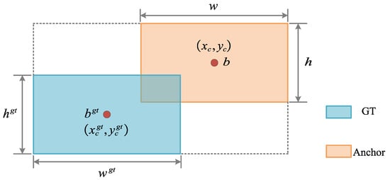
Figure 6.
Schematic of the ShapeIoU loss. The loss augments with direction-aware shape distance and penalties to improve contour alignment and localization stability on tiny targets.
The metric (overlap between the predicted and ground-truth boxes) is defined as
where B and denote the predicted and ground-truth bounding boxes, respectively. The computation of ShapeIoU is given by Equations (11)–(17):
where is a shrinkage factor related to the proportion of small targets in the dataset; and are the horizontal and vertical weights determined by the aspect ratio of the ground-truth box; and and are the width and height of the ground-truth box.
where is the shape-distance term; and are the center coordinates of the predicted and ground-truth boxes; c is the diagonal length of the ground-truth box; is a shape penalty; and are dynamic weights; and denotes the direction-specific weight ().
The final bounding-box regression loss of ShapeIoU is
Compared with CIoU, ShapeIoU provides direction-aware penalties on shape and aspect-ratio mismatches, yielding more stable localization on tiny, shape-diverse targets under yellow-board conditions. In our setting, this improves contour alignment and box-shape consistency, which supports higher recall while avoiding false positives, aligning with the early-warning objective that emphasizes both recall and precision.
3.1.4. Network Slimming
The dataset in this study contains only one class: ACP on yellow-board. Although the P2 + P3 reconfiguration reduces the number of parameters and the model size, the introduction of the high-resolution P2 branch increases computation. Therefore, further channel pruning is required to lower computational cost and to enable efficient edge deployment for an ACP early-warning network.
The core idea of Network Slimming [] is to exploit the batch-normalization (BN) scaling factor associated with each channel and to train these factors jointly with the network weights. For a BN layer with C channels, given the pre-normalized activations and the batch statistics , the normalized output of channel c is
where and are the learnable scale and bias, and is a small constant for numerical stability. Thus, each serves as a multiplicative gate on the corresponding feature channel: when is small, the contribution of that channel to downstream layers is effectively suppressed. A sparsity regularization is imposed on the scaling factors so that some of them are driven close to zero, providing a criterion for channel importance. The structure is shown in Figure 7; during pruning, channels with large scaling factors (solid lines) are kept, and channels with small factors (dashed lines) are removed. This process guides channel-level sparsity during training, provides an explicit measure of channel importance, and achieves structured compression.
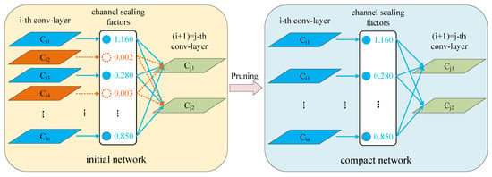
Figure 7.
Workflow of Network Slimming. Batch-normalization (BN) scaling factors guide channel-level sparsity during training; channels with small scales are pruned and the model is then fine-tuned to recover performance.
We jointly optimize the network weights and the channel scaling factors with the following training objective:
where denotes the training input and target, denotes the trainable weights, and the first summation term is the standard detection loss. The set contains the scaling vectors of all BN layers to be pruned, and the penalty encourages many channel-wise scales to move toward zero, yielding a sparse distribution over channels. In the pruning stage, we collect the absolute values from these layers, apply a global threshold or sparsity ratio, and remove channels whose falls below the criterion. For each pruned channel, the corresponding output channel of the preceding convolution and its BN parameters are deleted, and the matching input channel of the following convolution is also removed, so that entire feature maps are dropped rather than individual weights. This yields a compact, structurally pruned detector with reduced computation and memory footprint, while a brief fine-tuning stage restores detection performance.
3.2. Experimental Platform and Evaluation Metrics
3.2.1. Experimental Environment and Parameter Settings
To verify the effectiveness of the improved algorithm, ACP-YSTD was used for model training, validation, and testing. The dataset was split into training, validation, and test sets in an 8:1:1 ratio, yielding 480 training images, 60 validation images, and 60 test images.
The experimental environment was Windows 11 (64-bit). The CPU was an Intel Core i7-14700KF with 48 GB of RAM. The GPU was an NVIDIA RTX 4080 SUPER with 16 GB of VRAM. Experiments were conducted using Python 3.11 and PyTorch 2.5.1. The training hyperparameters are shown in Table 3.

Table 3.
Baseline training hyperparameters and evaluation settings on the ACP-YSTD dataset (unless otherwise specified).
3.2.2. Evaluation Metrics
After training and inference, strict quantitative evaluation was performed to assess the model’s effectiveness and robustness in object detection. The metrics include precision (P), recall (R), F1 score (F1), frames per second (FPS), number of parameters, floating-point operations (FLOPs), and model size. The formulas for precision, recall, and F1 are
In these formulas, true positive () denotes positive samples correctly predicted as positive; false positive () denotes negative samples incorrectly predicted as positive; and false negative () denotes positive samples incorrectly predicted as negative. The metric precision measures the proportion of correct predictions among all positive predictions, and recall measures the proportion of correctly detected positives among all positives that should be detected. F1 is the harmonic mean of precision and recall and is often used as a comprehensive metric to balance them.
FPS measures runtime efficiency in practical applications and indicates how many image frames the model can process per second. The number of parameters reflects model complexity and storage needs. FLOPs quantify the number of floating-point operations required during inference. Model size denotes the disk footprint of the exported weight file (e.g., MB) and is directly related to download, transfer, and on-device storage during deployment. All metrics were measured under the same hardware environment and input-size conditions as the comparison models to ensure comparability.
3.3. Algorithm of the Proposed Method
The overall training and pruning pipeline of TGSP-YOLO11 can be summarized as follows:
- Step 1:
- Initialize the network structure by taking YOLO11n as the baseline and modifying it to obtain the unpruned TGSP-YOLO11: reconfigure the detection head to the two-scale P2 + P3 design, insert the GSF module for high-resolution feature fusion, and replace CIoU with ShapeIoU as the bounding-box regression loss.
- Step 2:
- Train the unpruned TGSP-YOLO11 without channel-sparsity regularization until the performance converges, and save the weights that achieve the best results on the validation data as the starting point for subsequent pruning.
- Step 3:
- Starting from these weights, continue training the model while augmenting the loss with an regularization term on the BN channel scaling factors , so that many channel-wise scales are gradually driven toward zero and a sparse distribution of BN scales is obtained across channels.
- Step 4:
- Collect the channel scaling factors from all prunable BN layers, determine a pruning threshold or target pruning ratio based on their absolute values , and remove channels whose scales fall below the chosen criterion. For each removed channel, delete the corresponding output channel and BN parameters in the preceding convolution, as well as the matching input channel in the following convolution, so that entire feature maps are discarded rather than individual weights, yielding a structurally pruned network.
- Step 5:
- Further train the pruned TGSP-YOLO11 without additional sparsity regularization to restore overall performance, and use the resulting pruned model as the final TGSP-YOLO11 in the experiments.
4. Results and Analysis
4.1. Effectiveness Analysis of the Two-Scale Feature Reconfiguration Network
To verify the advantages of the two-scale feature reconfiguration for tiny objects in this task, we conducted comparative experiments under the same data split, training strategy, and input size (), changing only the detection head configuration (see Table 4). The four structures were: P3 + P4 + P5 (three-head baseline), P2 + P3 + P4 + P5 (four-head full), P2 + P3 + P4 (removing P5), and P2 + P3 (the two-scale reconfiguration proposed in this work). The evaluation focused on precision, recall, and F1, and also reported parameters, model size, and GFLOPs to measure deployment cost.

Table 4.
Ablation of detection head configurations on the ACP-YSTD test set (input ). Best results are highlighted in bold.
The results show that P2 + P3 better fits pest early-warning scenarios that prioritize recall: compared with the three-head baseline (P3 + P4 + P5), recall increases from 90.9% to 93.7% (+2.8 percentage points), and F1 increases from 91.5 to 92.0 (+0.5); precision decreases slightly from 92.2% to 90.4%, which is an acceptable trade-off under a high-recall-first strategy. Compared with the four-head full (P2 + P3 + P4 + P5), P2 + P3 achieves a similar overall accuracy with fewer parameters and lower computation: F1 is 92.0 (92.2 for the four-head), but recall is higher (93.7% vs. 92.9%); at the same time, parameters drop from 2.659 million to 1.709 million, model size from 6.0 MB to 4.0 MB, and GFLOPs from 10.2 to 9.0. Compared with P2 + P3 + P4, P2 + P3 increases recall and F1 to 93.7% and 92.0, respectively, and reduces GFLOPs from 9.6 to 9.0, indicating that retaining only the higher-resolution P2 + P3 scales better matches the target size distribution of ACP-YSTD; in this task, keeping P4 as a detection head provides no additional benefit.
It should be noted that, relative to the three-head baseline, all structures including P2 show increased GFLOPs. This arises from the inherent computational cost of the high-resolution branch and is a necessary investment to improve the detectability of tiny objects. Subsequent sections will further compress computational redundancy and deployment cost through lightweight fusion (GSF) and structured pruning (Network Slimming), and will alleviate the slight precision decrease introduced by the high-resolution branch, enabling the model to maintain high recall while balancing engineering efficiency and deployability at the edge.
4.2. Effectiveness Analysis of the GSF Module
GSF aims to suppress the texture and stain noise introduced by the high-resolution branch (P2) in the two-scale network (P2 + P3), while preserving fine-grained detail features that benefit tiny objects. The module comprises two parts: (1) adaptive non-negative normalized weights for the two-scale branches; and (2) a main-branch residual controlled by coefficient , which provides a stabilizing correction at fine-grained boundaries. To examine the effect of residual strength on performance, we extend the sweep of to (step 0.05), and report the results in Table 5. The extended range shows that an excessively large imposes over-constraint on cross-scale fusion and weakens complementary cues from P3, whereas a small but non-zero stabilizes boundary-level corrections without drowning the adaptive weights.

Table 5.
Effect of the GSF residual strength () in two-scale fusion (P2 + P3) on the ACP-YSTD test set (input ). Best results are highlighted in bold.
As shown in Table 5, GSF significantly improves the overall detection performance of the two-scale network with almost no increase in parameters or computation. First, even at (adaptive weighting only, no residual), precision, recall, and F1 reach 91.5%, 93.9%, and 92.7, all higher than the two-scale reconfiguration baseline of 90.4%, 93.7%, and 92.0, indicating that adaptive weighting effectively suppresses the interference of high-resolution noise. Furthermore, performance is optimal when is in a moderate range: at , precision rises to 94.0%, recall remains at 92.9%, and F1 reaches the highest value of 93.4, forming a more balanced precision–recall relationship. When is too small (e.g., 0.10), the correction is insufficient and F1 drops to 90.8; once exceeds approximately 0.30, a general downward trend of F1 emerges—with minor local fluctuations (e.g., at 0.45)—because the residual starts to dominate and limits cross-scale information flow. With the extended sweep (), recall becomes more sensitive than precision (e.g., at ), and F1 stabilizes at a lower plateau around (0.50–0.80), reflecting over-suppression of fused details and the relative reemergence of P2 noise. Considering all factors, we set as the default: it maintains high recall, significantly improves precision, and pushes F1 to its peak, verifying the effectiveness of GSF in yellow-board scenarios with dense tiny targets, diverse shapes, and frequent specular interference while preserving the fine-detail features required for high recall.
4.3. Effectiveness Analysis of the ShapeIoU Loss Function
Under fixed network structure and training configuration, we replace only the bounding-box regression loss for comparison; results are shown in Table 6. ShapeIoU [] achieves precision, recall, and F1 of 93.2%, 94.0%, and 93.6; CIoU [] achieves 94.0%, 92.9%, and 93.4; the other candidate losses (Focal-EIoU [], GIoU [], InnerIoU [], DIoU [], WIoU []) are overall lower than these two. ShapeIoU maintains high precision while raising recall to the highest in the table and achieving the best F1. Compared with CIoU, precision decreases slightly by 0.8 percentage points, but recall increases by 1.1 percentage points, leading to a better overall metric. This aligns with the “report upon detection” requirement of pest early warning: under reasonable precision, reducing missed detections is prioritized.

Table 6.
Comparison of bounding-box regression losses under identical architecture and training schedule on the ACP-YSTD test set (input ). Best results are highlighted in bold.
The root cause of this difference lies in the match between data and mechanism. Targets in ACP-YSTD are mainly tiny (at 960 input, average width and height are about twenty pixels). Specular reflection, stains, and slight occlusion on yellow-board can induce small boundary shifts. CIoU mainly constrains center distance and aspect ratio, and its characterization of “shape inconsistency” is insufficient. On tiny objects, even pixel-level deformation and alignment error can cause noticeable IoU fluctuations, making missed detections more likely during training. ShapeIoU introduces shape distance and direction-sensitive weights on top of IoU, adaptively penalizing horizontal and vertical mismatches. It aligns contours and boxes more robustly, reducing matching failures caused by slight deformations. Combined with the two-scale feature reconfiguration (P2 + P3) and the high-resolution fine-detail representation provided by GSF, ShapeIoU strengthens localization robustness for tiny objects, allowing more positive samples to pass the threshold, thereby improving recall and increasing F1 in a more balanced way. Meanwhile, replacing the loss acts only during training and introduces no extra computation or parameters at inference, preserving the efficiency required for edge deployment.
Based on the above results and mechanism analysis, the final model adopts ShapeIoU instead of CIoU to obtain higher recall and better overall detection performance, which better fits the core requirement of pest monitoring and early warning to control missed detections.
4.4. Effectiveness Analysis of Network Slimming
To verify the role of channel-sparsity-based pruning in this task, we completed the full pipeline of sparse training → pruning → fine-tuning using the Network Slimming hyperparameters in Table 7, and we systematically scanned pruning rates from 0.1 to 0.9. This pipeline works in conjunction with the two-scale structure (P2 + P3), GSF, and ShapeIoU. The goal was to significantly reduce parameters and computation while ensuring the high recall required for pest early warning, thereby improving the feasibility of edge deployment.

Table 7.
Network Slimming experimental hyperparameter settings.
Figure 8 shows the distribution of BN scaling factors during normal training (0–100 epochs). The curve is concentrated and sharp, with the main peak around 1, and it almost lacks discriminability, making it difficult to judge channel importance. After introducing sparse regularization, Figure 9 shows that within 0–500 epochs the distribution of gradually spreads apart and eventually forms a bimodal structure near 0 and close to 1: channels with near 0 were continuously suppressed (prunable channels), indicating limited contribution to target discrimination; channels with near 1 maintained high responses (important channels) that should be retained. This differentiation directly provides an actionable pruning basis, making subsequent threshold selection and consistent processing across the network more reliable.
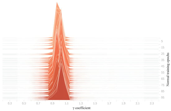
Figure 8.
Distribution of BN-layer coefficients during normal training (0–100 epochs).
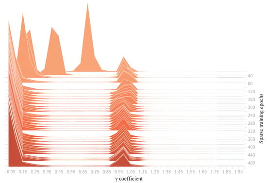
Figure 9.
Distribution of BN-layer coefficients during sparse training (0–500 epochs).
Using a pruning rate of 0.8 as an example, the channel comparison (Figure 10) shows that the number of channels is significantly reduced in most layers, and the compression is not concentrated in only a few layers but distributed across multiple key nodes of the network. The pruned channels are mainly those whose values have shrunk toward zero. This indicates that the prunable channels identified during sparse training were accurately removed at the structural level, effectively slimming the high-resolution branch (especially the early and middle convolutional layers with higher computational cost) and laying the foundation for subsequent reductions in computation and storage overhead.

Figure 10.
Channel comparison before and after pruning (pruning rate 0.8).
Table 8 summarizes the changes in scale and performance as the pruning rate varies from 0 to 0.9. Compared with the unpruned model (parameters 1,711,996, model size 4.0 MB, GFLOPs 9.1, precision 93.2%, recall 94.0%, F1 93.6), a pruning rate of 0.7 achieves the highest F1 (94.1) in this group, while parameters and GFLOPs drop to 542,858 and 6.5, showing that a higher compression ratio can still yield better overall accuracy. When further increased to 0.8, recall rises to the highest in the table at 95.5%, accompanied by more aggressive compression: parameters 392,591 (a reduction of 1,319,405 from the unpruned model, down 77.1%), model size 1.4 MB (down 2.6 MB, 65.0%), and GFLOPs 6.0 (down 3.1, 34.1%). At this point, F1 is 93.9, an increase of 0.3 over the unpruned model, and precision drops slightly from 93.2% to 92.4%. When the pruning rate reaches 0.9, model capacity becomes insufficient and F1 falls to 76.6, indicating clear degradation and suggesting a reasonable upper limit to pruning.

Table 8.
Effect of pruning rate on model scale and detection performance on the ACP-YSTD test set (input ) after fine-tuning. Best results are highlighted in bold.
To further demonstrate the performance–cost advantage of Network Slimming, we compare it with three classical pruning methods—-norm filter pruning (PFEC) [], Layer-Adaptive Magnitude-based Pruning (LAMP) [], and Group- norm structured pruning (DepGraph) []. For fairness, all methods are aligned to the same compute budget of 6.0 GFLOPs, an identical fine-tuning schedule is used, and evaluation is conducted on the ACP-YSTD test set with 960 × 960 input.
As shown in Table 9, at the same compute budget (6.0 GFLOPs), Network Slimming yields precision 92.4%, recall 95.5%, and F1 93.9. Relative to LAMP, F1 increases by 2.5, recall increases by 4.2 percentage points, and precision increases by 0.9 percentage points; the margins over PFEC and DepGraph are larger. This indicates that BN scaling factor -guided channel-level structured pruning better preserves tiny-object–critical pathways across P2 + P3 while coherently removing low-saliency channels network-wide. In contrast, PFEC tends to over-prune early high-resolution filters that encode fine spatial cues, and DepGraph can introduce irregular connectivity that is harder to fine-tune and less inference-friendly on edge hardware. Although LAMP remains competitive, its lower recall at the same GFLOPs suggests that per-layer magnitude adaptation is less aligned with the cross-scale semantics required by yellow-board tiny-target detection. Overall, under the same compute constraint, Network Slimming lies on the Pareto frontier of F1 vs. GFLOPs (i.e., no alternative simultaneously dominates it in both accuracy and compute).

Table 9.
Pruning method comparison at a matched compute budget (6.0 GFLOPs) on the ACP-YSTD test set (input 960 × 960). Best results are highlighted in bold.
Combining the distribution differentiation in Figure 8 and Figure 9 with the channel comparison before and after pruning in Figure 10, sparse training clearly separates prunable channels from important channels at both statistical and structural levels. Together with the scan results in Table 8, this study prioritized recall and deployment efficiency for the “report upon detection” early-warning scenario and finally selected a pruning rate of 0.8: while maintaining a high F1, it pushes recall to the highest value of 95.5% and brings a 77.1% reduction in parameters, a 65.0% reduction in model size, and a 34.1% reduction in computation. Moreover, the matched-compute comparison in Table 9 shows that, at the same 6.0 GFLOPs, Network Slimming attains precision 92.4%, recall 95.5%, and F1 93.9, outperforming PFEC, LAMP, and DepGraph by clear margins. Thus, Network Slimming in this task satisfies both detection stability and engineering lightweight requirements, providing solid support for building a large-scale pest monitoring and protection network at the orchard edge.
4.5. Ablation Study Results Analysis
Under a consistent data split and training pipeline, we conducted a stepwise additive evaluation of two-scale reconfiguration (P2 + P3), GSF, ShapeIoU, and Network Slimming; results are shown in Table 10. The first row corresponds to the original YOLO11n detector with the conventional three-scale head (P3 + P4 + P5), CIoU as the bounding-box regression loss, and no GSF or Network Slimming. In the second row, only the detection head is reconfigured to the two-scale P2 + P3 design while keeping the backbone, neck, and loss unchanged. The third row further inserts the GSF module into the fusion path between P2 and the upsampled P3 feature maps. The fourth row then replaces CIoU with ShapeIoU for box regression. Finally, the last row applies Network Slimming with a pruning rate of 0.8 to this configuration, yielding the compact TGSP-YOLO11 model.

Table 10.
Ablation study of P2 + P3, GSF, ShapeIoU, and Network Slimming on the ACP-YSTD test set (input ). “✓” indicates the module is used. Best results are highlighted in bold.
Starting from the three-head baseline (precision = 92.2%, recall = 90.9%, F1 = 91.5; parameters 2,582,347; model size 5.5 MB; GFLOPs 6.3), lowering the detection heads to P2 + P3 raises recall from 90.9% to 93.7% and F1 to 92.0; meanwhile, parameters drop by 33.8% and model size drops by 27.3%. However, because the high-resolution branch introduces more background textures and stain details, precision decreases from 92.2% to 90.4%, and computation rises to 9.0 GFLOPs. This stage aligns with the method’s motivation: P2 enhances the visibility and recall of tiny objects but is more sensitive to noise.
After adding GSF on the two-scale structure, precision increases to 94.0%, F1 rises to 93.4, and recall is 92.9%. Compared with using P2 + P3 only, precision improves by 3.6 percentage points and F1 by 1.4, while recall remains higher than the three-head baseline. Parameters and model size remain essentially unchanged (1,711,996; 4.0 MB), and GFLOPs increase slightly to 9.1. This indicates that adaptive weighting suppresses P2 noise amplification, while the residual term provides a stabilizing correction at fine-grained boundaries, thereby restoring and strengthening precision while maintaining the fine-detail features required for high recall.
On this basis, replacing CIoU with ShapeIoU increases recall to 94.0% and F1 to 93.6, with precision slightly falling to 93.2%. Relative to the previous row, recall increases by 1.1 percentage points and F1 by 0.2; this replacement acts only during training and does not add computation or parameters at inference. Consistent with the earlier mechanism, the shape distance and direction-sensitive weights of ShapeIoU align tiny-object contours more robustly, mitigating matching failures caused by slight deformations, thereby improving recall and yielding a more balanced overall metric.
Introducing Network Slimming (pruning rate 0.8) while keeping the two-scale structure, GSF, and ShapeIoU unchanged reduces parameters from 1,711,996 to 392,591 (down 77.1%), model size from 4.0 MB to 1.4 MB (down 65.0%), and GFLOPs from 9.1 to 6.0 (down 34.1%). Precision is 92.4%, recall increases to 95.5%, and F1 is 93.9. Compared directly with the three-head baseline, parameters drop from 2,582,347 to 392,591 (down 84.8%), model size from 5.5 MB to 1.4 MB (down 74.5%), and GFLOPs from 6.3 to 6.0 (down 4.8%); meanwhile, precision increases by 0.2 percentage points (92.2 to 92.4), recall increases by 4.6 percentage points (90.9 to 95.5), and F1 increases by 2.4 (91.5 to 93.9). This shows that sparsity-induced structured pruning effectively removes redundant channels, focusing feature expression on salient cues related to ACP and maintaining or even improving detection performance while reducing computational cost.
Overall, the ablation results present a clear progressive relationship: P2 + P3 improves the visibility of tiny objects and increases recall; on this basis, GSF suppresses high-resolution noise and strengthens precision, driving F1 upward; ShapeIoU further stabilizes geometric alignment, continuing to improve recall and overall performance; Network Slimming greatly compresses parameters, model size, and computation, while pushing recall to the highest level and maintaining a high F1. The final configuration meets the “report upon detection” business requirement and significantly reduces resource usage, making large-scale edge deployment in orchards feasible.
4.6. Model Comparison Experiments
To verify the overall advantages of the proposed method in yellow-board ACP detection, we compared representative detectors; results are shown in Table 11. The proposed method (TGSP-YOLO11) achieves the best recall and F1 in the table while maintaining low parameters and computation: precision 92.4%, recall 95.5%, F1 93.9, parameters 392,591, model size 1.4 MB, GFLOPs 6.0.

Table 11.
Model comparison on the ACP-YSTD test set (input ). Best results are highlighted in bold.
Compared with models from the same family, the main gains are clear. Relative to YOLO11n [], precision is essentially unchanged (92.2% to 92.4%); meanwhile, recall increases from 90.9% to 95.5% (+4.6%), and F1 from 91.5 to 93.9 (+2.4). After that, parameters drop from 2,582,347 to 392,591 (down 84.8%), model size from 5.5 MB to 1.4 MB (down 74.5%), and GFLOPs from 6.3 to 6.0 (down 4.8%). Compared with YOLOv12n [] and YOLOv13n [], under an approximate 6 GFLOPs budget, recall increases by 6.9 and 5.7 percentage points, and, correspondingly, F1 increases by 3.6 and 3.9; parameter reductions are about 84–85%, and model size reductions are about 74–75%. These comparisons indicate that, under a low-compute budget of about 6 GFLOPs, TGSP-YOLO11 improves accuracy not by increasing depth or width, but by concentrating capacity and computation on task-relevant components: the P2 + P3 head shifts detection toward higher-resolution feature maps that match the 6–40 pixel scale of ACP targets, GSF suppresses yellow-board texture and stain noise on the high-resolution branch while preserving fine-grained insect cues, ShapeIoU enhances localization stability for tiny boxes without adding inference cost, and Network Slimming removes redundant channels so that the remaining parameters are mainly devoted to ACP-related features, enabling higher recall and F1 with a much smaller model.
The advantages are also stable against other lightweight models. Compared with YOLOv8n [] and YOLOv10n [], recall increases by 10.1 and 4.6 percentage points, and F1 improves by 6.0 and 5.6; at the same time, parameters decrease by about 87.0% and 85.4%, model size decreases by 77.8% and 75.9%, and GFLOPs decrease by 25.9% (8.1 to 6.0) and 26.8% (8.2 to 6.0). For the “tiny” series, compared with YOLOv7-tiny [] (recall 87.0%, F1 88.8; parameters 6,007,596; GFLOPs 13.0) and YOLOv9-tiny [] (recall 89.2%, F1 91.3; parameters 2,616,950; GFLOPs 10.7), the proposed method raises recall by 8.5 and 6.3 percentage points and improves F1 by 5.1 and 2.6, while reducing parameters by about 93.5% and 85.0%, reducing model size by 88.6% and 77.4%, and reducing GFLOPs by 53.8% and 43.9%. It can be seen that simply enlarging or deepening a lightweight backbone cannot effectively overcome the scenario challenge of “tiny objects + specular/stain noise”; task-oriented structure and loss design are more critical.
We also make a lateral observation against methods with markedly different architectural styles. SSD [] has recall of 61.6 and F1 of 74.0, with computation and parameter costs clearly higher than the proposed method. RT-DETR [], under the given data scale and target size, has recall of 76.5 and F1 of 79.0, while requiring 103.4 GFLOPs and 31,985,795 parameters, which is difficult to meet edge deployment constraints. This comparison shows that in the yellow-board scenario—“uniform background but prone to specular interference”—the combination of two-scale representation for tiny targets and structured pruning better matches task needs and engineering limits.
For an intuitive performance–cost view, Figure 11 maps recall, computation, and parameter count to the vertical axis, horizontal axis, and circle radius, respectively. The bubble for the proposed method lies in the upper-left region with a smaller radius: it achieves the highest recall under an approximately 6 GFLOPs budget. With a zoomed-in view, it is clearly separated from YOLO11n, YOLOv12n, and YOLOv13n, showing a recall advantage under smaller parameters and slightly lower computation.
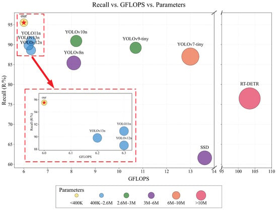
Figure 11.
Performance visualization across models on the ACP-YSTD test set (input ). Vertical axis: recall; horizontal axis: GFLOPs; circle size: number of parameters. Closer to the upper-left with smaller circles indicates better recall at lower computation and smaller model size.
For a more fine-grained view of detector behavior across confidence thresholds, Figure 12 presents the Precision–Recall (PR) curves of all models in Table 11 on the ACP-YSTD test set. In this single-class, dense small-object detection setting, the number and definition of true negatives at the pixel or proposal level are ambiguous and heavily imbalanced, so PR curves provide a more informative characterization than ROC curves. Overall, most detectors maintain high precision when recall is moderate, but as recall approaches the high-recall regime required by “report upon detection” early warning, the curves separate. SSD and RT-DETR exhibit a pronounced drop in precision as recall increases, while lightweight YOLO variants such as YOLOv7-tiny, YOLOv8n, and YOLOv10n also degrade noticeably. YOLO11n, YOLOv12n, and YOLOv13n remain closer to the top-right region, but TGSP-YOLO11 consistently lies on or near the upper envelope of all curves, maintaining higher precision at recall levels around 0.9 and above. This is consistent with its leading F1 score under an approximately 6 GFLOPs computation budget.
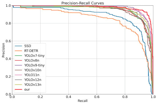
Figure 12.
Precision–Recall curves of the detectors on the ACP-YSTD test set (input ). Vertical axis: precision; horizontal axis: recall. Curves closer to the upper-right indicate a more favorable precision–recall trade-off, especially in the high-recall regime required for early warning.
To complement the above detector-level comparison, we also examined whether the performance gains can be reproduced simply by replacing the backbone with recent classification networks. Concretely, we constructed three YOLO11n variants by swapping the original backbone for MobileViT V2 [], Swin Transformer [], and ConvNeXt V2 [], while keeping the neck, detection heads, and training settings unchanged, and evaluated them under the same input on ACP-YSTD. The results are summarized in Table 12.

Table 12.
Backbone-swapped comparison under a unified YOLO11n detector on the ACP-YSTD test set (input ). Only the backbone is replaced; neck, detection heads, and training settings remain unchanged. Best results are highlighted in bold.
From Table 12, simply swapping in recent backbones does not consistently improve the detector over YOLO11n. MobileViT V2 gives the highest F1 among the swapped variants, reaching 91.2, which is close to the YOLO11n baseline of 91.5. However, this variant increases parameters to about 3.0M and model size to 6.5 MB, and its computation rises to 9.8 GFLOPs, which is roughly 63% higher than the 6.0 GFLOPs of the proposed method. Swin Transformer attains the highest recall among the swapped models at 92.3%, but its precision drops to 88.5%, so the F1 score is only 90.4. ConvNeXt V2 shows the lowest overall accuracy, with precision 89.3%, recall 88.0%, and F1 88.6, despite a compute budget similar to YOLO11n. In contrast, TGSP-YOLO11 achieves precision 92.4%, recall 95.5%, and F1 93.9 with only 392,591 parameters and a model size of 1.4 MB at 6.0 GFLOPs. Compared with MobileViT V2, recall increases by 5.0 percentage points and F1 increases by 2.7, while parameters and model size are reduced by about 87% and 78%, and computation is reduced from 9.8 to 6.0 GFLOPs. Compared with Swin Transformer, recall increases by 3.2 percentage points and F1 by 3.5, with about 84% fewer parameters and a comparable compute budget. Compared with ConvNeXt V2, recall increases by 7.5 percentage points and F1 by 5.3 at similar computation. These results show that on ACP-YSTD, recent classification backbones do not close the performance gap when directly plugged into the YOLO11n framework, whereas the task-oriented redesign of the detection head, fusion, loss, and pruning in TGSP-YOLO11 yields higher recall and F1 under a tighter parameter and model-size budget.
Further qualitative comparisons are shown in Figure 13. Three methods near the upper-left of the plot are used to visualize detections on the same images: in (a), YOLO11n and YOLOv13n each miss one target and produce two false positives; in (b), YOLO11n misses one target and produces three false positives, and YOLOv13n misses one target and produces one false positive. The proposed method detects all targets in both images, with significantly fewer false positives.
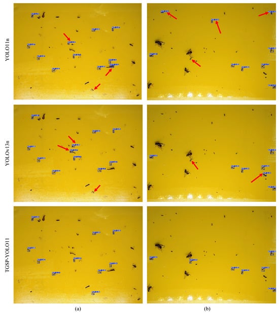
Figure 13.
Qualitative comparison on ACP-YSTD. Panels (a) and (b) are images from the ACP-YSTD dataset; detections from YOLO11n, YOLOv13n, and TGSP-YOLO11 are shown on the same images. Red arrows indicate missed and false detections.
In summary, the statistics in Table 11, the backbone-swapped comparison in Table 12, and the visualizations in Figure 11, Figure 12 and Figure 13 corroborate each other. Under a unified setup, TGSP-YOLO11 consistently achieves the highest recall and F1 while keeping parameters, model size, and computation at levels suitable for edge deployment. The PR-curve analysis further confirms that in the high-recall regime required for “report upon detection” early warning, TGSP-YOLO11 maintains a favorable precision–recall trade-off compared with the other detectors. The additional backbone experiments indicate that simply enlarging or updating the backbone does not reproduce these gains; instead, the main improvements come from the two-scale detection head, noise-suppressed fusion, shape-aware regression, and structured pruning. For the specific application of yellow-board ACP detection, TGSP-YOLO11 achieves a more favorable balance between detection reliability and resource consumption and is suitable for large-scale, long-term deployment for pest early warning at the orchard edge.
4.7. Transfer Experiments
To verify the actual detection performance and generalization ability of TGSP-YOLO11, we additionally collected 20 yellow-board images at the experimental site for an independent evaluation (partial results are shown in Figure 14). To ensure rigor in the transfer evaluation, the sample size was set to a single independent field batch collected after model freezing and outside the ACP-YSTD time window. The batch includes all yellow-board images that passed quality control within one complete on-site acquisition pass (20 images), avoiding any post hoc selection. This provides a sufficient number of target instances for error inspection and metric verification without additional data collection. The acquisition and labeling protocols are identical to those of ACP-YSTD, ensuring comparability without conflating datasets. These images contain 262 ACP in total, and the model detected 251. The precision, recall, and F1 of the transfer experiment are 94.3%, 95.8%, and 95.0, respectively. Compared with the ACP-YSTD test set (precision 92.4%, recall 95.5%, F1 93.9), these values are at least comparable and slightly higher, indicating that TGSP-YOLO11 does not exhibit noticeable performance degradation on unseen yellow-board images collected at a different time. In this independent batch, the model captures the vast majority of ACP individuals while keeping false alarms at a low level, which is consistent with the early-warning requirement of “report upon detection and minimize misses.”
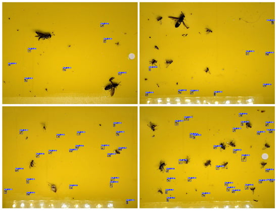
Figure 14.
Qualitative results of the transfer experiment. TGSP-YOLO11 is applied to an independent orchard set (20 yellow-board images not seen during training), distinct from the ACP-YSTD dataset.
Inference efficiency is also evaluated. Under the same environment, we repeated inference for 5 rounds. The average frame rate of TGSP-YOLO11 is 159.2 FPS, which is 11.6 FPS higher than YOLO11n at 147.6 FPS (+7.9%). With higher recall and better overall metrics, it also achieves faster inference speed, meeting real-time monitoring requirements.
It should be emphasized that TGSP-YOLO11 maintains the extremely low parameter count and model size brought by the aforementioned structure and pruning design (about parameters, 1.4 MB; GFLOPs 6.0). This significantly reduces storage and computation pressure on devices during multi-site, long-term online deployment at the orchard edge. Network-side data distribution and remote maintenance costs are also lowered, facilitating the construction of a high-density, low-cost monitoring and early-warning network.
In summary, the transfer experiment shows that TGSP-YOLO11 maintains stable detection quality and high inference efficiency on new, previously unseen yellow-board images. The recall advantage is further demonstrated, precision remains reliable, and speed meets real-time applications, while the model size and computation stay within an edge-friendly budget. These results, together with the main test-set evaluation, indicate that the proposed method generalizes well under temporal shifts in field data and is suitable for long-term deployment in real orchard environments.
5. Discussion
Under unified acquisition and annotation procedures, this study has achieved high recall and robust overall performance in the task of yellow-board ACP detection. Owing to the stickiness of the yellow-board surface and the transfer process, occasional adhesion between boards occurs during field collection, increasing the operational difficulty of batch transfer and sample management. To ensure imaging stability and annotation quality, this work adopts a “retrieval–laboratory imaging” pipeline, which represents a rational trade-off between quality and operability. On this basis, future work may be moderately expanded to multi-site on-site acquisition, and simple anti-sticking measures such as separation liners, trays, and numbering can be used during recovery, so as to progressively broaden spatial coverage without altering the advantages of the existing workflow and further enhance the dataset’s generalization capacity. Concretely, in the next data-collection phase we will conduct cross-scenario on-site acquisition in 3–5 representative citrus-growing regions (e.g., South and East China), targeting at least 50 yellow-board images per region within a single maintenance cycle under the same imaging and labeling protocol; in parallel, we will introduce controlled data augmentations (e.g., illumination range, stain intensity) to emulate field variations without changing the deployment-oriented workflow. We will also extend the annotation schema to record key ACP attributes such as developmental stage (e.g., nymph/adult) as auxiliary tags to enable attribute-aware analysis and reporting, while keeping the detector’s class definition unchanged.
Meanwhile, the present 8:1:1 split (480/60/60) leaves a relatively small validation and test set, which may limit statistical confidence for rare edge cases; our transfer evaluation on newly acquired orchard images mitigates this concern to some extent. As a future step to further improve robustness and statistical reliability, we plan to adopt image-level k-fold cross-validation (with stratification by ACP counts/density and board identity constraints) while keeping the current deployment-oriented workflow unchanged, and to report the variability of precision, recall, and F1 across folds for a more systematic validation of the observed gains.
At the model level, knowledge distillation is expected to provide a small yet stable performance gain without increasing the parameter count, model size, or computation at inference. However, distillation typically requires a high-capacity teacher model and substantially increases memory and compute demands during training, so a comprehensive distillation study is left for future work, when upgraded hardware will make training such teacher–student configurations more practical. At that point, distillation can be incorporated into the existing framework as a gain-oriented improvement that does not add deployment burden, further consolidating recall and overall detection metrics. These potential improvements are iterative refinements to the current system and do not alter the main conclusions and practical value regarding high recall, lightweight design, and edge deployability.
6. Conclusions
This study proposes TGSP-YOLO11 for the yellow-board ACP edge-deployment scenario. It addresses key issues such as missed detections of tiny targets, noise amplification from texture/stain interference, unstable localization and alignment, and deployment resource constraints. While ensuring lightweight design and deployability, it significantly enhances detection reliability and practicality.
First, a high-quality ACP-YSTD dataset was built (unified background and acquisition process, covering common interference factors) to provide a standardized data basis for subsequent training and evaluation. TGSP-YOLO11 is proposed on the YOLO11 backbone with the following improvements: the detection head is reconfigured to two scales (P2 + P3) to match target size and reduce redundant paths; GSF is introduced to suppress noise amplification and false positives; ShapeIoU is adopted for better shape and alignment of tiny targets; and Network Slimming is used for channel-level pruning, reducing parameters, FLOPs, and model size while maintaining detection performance, addressing the resource constraints of long-term edge-side monitoring.
On the ACP-YSTD test set, TGSP-YOLO11 achieves precision 92.4%, recall 95.5%, and F1 93.9, with 392,591 parameters, a model size of 1.4 MB, and 6.0 GFLOPs. Compared with YOLO11n, recall increases by 4.6%, F1 increases by 2.4, and precision increases by 0.2%; meanwhile, the parameter count decreases by 84.8%, the model size decreases by 74.5%, and the computation decreases by 4.8%. Compared with other representative models, the recall of TGSP-YOLO11 is higher than that of SSD, RT-DETR, YOLOv7-tiny, YOLOv8n, YOLOv9-tiny, YOLOv10n, YOLOv12n, and YOLOv13n by 33.9%, 19.0%, 8.5%, 10.1%, 6.3%, 4.6%, 6.9%, and 5.7%, respectively; F1 is higher by 19.9, 14.9, 5.1, 6.0, 2.6, 5.6, 3.6, and 3.9, respectively; and the parameter count, model size, and computation are reduced by 84.0–98.8%, 74.5–97.9%, and 3.2–94.2%, respectively. In the transfer experiment for practical application evaluation (20 independent yellow-board images with a total of 262 individuals), TGSP-YOLO11 attains precision 94.3%, recall 95.8%, F1 95.0, and FPS 159.2.
Overall, TGSP-YOLO11 achieves faster inference, lower deployment cost, higher recall, and better overall metrics, making it suitable for real-time monitoring and pest early warning at the orchard edge, with strong potential for large-scale deployment.
Author Contributions
Conceptualization, L.C., X.L. and Z.W.; methodology, L.C., W.X. and H.C.; software, W.X. and X.L.; validation, L.C., W.X. and H.C.; formal analysis, L.C. and W.X.; investigation, W.X., Y.M. and S.Z.; resources, L.C., W.X. and Z.W.; data curation, W.X., X.L. and Z.W.; writing—original draft preparation, W.X. and Z.W.; visualization, W.X. and Z.W.; supervision, L.C., X.L. and Z.W.; project administration, L.C., X.L. and H.C.; funding acquisition, L.C. and Z.W. All authors have read and agreed to the published version of the manuscript.
Funding
This paper was supported partly by Special projects in key areas for ordinary colleges and universities in Guangdong Province under Grant 2023ZDZX4014 and 2023ZDZX4015, Guangdong Provincial University Innovation Team Project (2025KCXTD022), Guangdong Provincial Graduate Education Innovation Plan Project under Grants 2022XSLT056 and 2024JGXM_093, Science and Technology Planning Project of Yunfu under Grant 2023020203, Open Competition Program of Top Ten Critical Priorities of Agricultural Science and Technology Innovation for the 14th Five-Year Plan of Guangdong Province (2022SDZG06, 2023SDZG06, and 2024KJ29), Innovation Team Project of Universities in Guangdong Province under Grant 2021KCXTD019, Guangzhou Science and Technology Program 201903010043, Guangdong Province key construction discipline Scientific Research Capacity Improvement Program (2021ZDJS001), and Guangdong Special Support Program for Young Top-notch Talents (NYQN2024013).
Data Availability Statement
Detailed descriptions of all essential experimental methods and analytical procedures are included herein. Additional data and materials can be obtained from the corresponding author upon reasonable academic request.
Conflicts of Interest
The authors declare no conflicts of interest.
Abbreviations
| ACP | Asian Citrus Psyllid |
| ACP-YSTD | Asian Citrus Psyllid Yellow Sticky Trap Dataset |
| F1 | F1 Score |
| Faster R-CNN | Faster Region-Based Convolutional Neural Networks |
| FLOPs | Floating-Point Operations |
| FN | False Negative |
| FP | False Positive |
| FPS | Frames Per Second |
| GSF | Guided Scalar Fusion |
| HLB | Huanglongbing |
| P | Precision |
| R | Recall |
| SSD | Single Shot MultiBox Detector |
| TN | True Negative |
| TP | True Positive |
| YOLO | You Only Look Once |
References
- Yan, K.; Song, X.; Yang, J.; Xiao, J.; Xu, X.; Guo, J.; Zhu, H.; Lan, Y.; Zhang, Y. Citrus huanglongbing detection: A hyperspectral data-driven model integrating feature band selection with machine learning algorithms. Crop Prot. 2025, 188, 107008. [Google Scholar] [CrossRef]
- Pérez-Hedo, M.; Hoddle, M.S.; Alferez, F.; Tena, A.; Wade, T.; Chakravarty, S.; Wang, N.; Stelinski, L.L.; Urbaneja, A. Huanglongbing (HLB) and its vectors: Recent research advances and future challenges. Entomol. Gen. 2025, 45, 17–35. [Google Scholar] [CrossRef]
- Dong, R.; Shiraiwa, A.; Ichinose, K.; Pawasut, A.; Sreechun, K.; Mensin, S.; Hayashi, T. Hyperspectral Imaging and Machine Learning for Huanglongbing Detection on Leaf-Symptoms. Plants 2025, 14, 451. [Google Scholar] [CrossRef]
- Xu, Q.; Su, Y.; Sun, L.; Cai, J. Detection of citrus Huanglongbing at different stages of infection using a homemade electronic nose system. Comput. Electron. Agric. 2025, 229, 109845. [Google Scholar] [CrossRef]
- Huang, D.; Xiao, K.; Luo, H.; Yang, B.; Lan, S.; Jiang, Y.; Li, Y.; Ye, D.; Sun, D.; Weng, H. Implementing transfer learning for citrus Huanglongbing disease detection across different datasets using neural network. Comput. Electron. Agric. 2025, 238, 110886. [Google Scholar] [CrossRef]
- Collins, C.F.; Oliver, J.E.; Barman, A.K.; Munoz, G.; Madrid, A.J. Confirmation of ‘Candidatus Liberibacter asiaticus’ in Asian Citrus Psyllids and Detection of Asian Citrus Psyllids in Commercial Citrus in Georgia (USA). Plant Dis. 2025, 109, 800–803. [Google Scholar] [CrossRef] [PubMed]
- Eduardo, W.I.; Cifuentes-Arenas, J.C.; Monteferrante, E.C.; Lopes, S.A.; Bassanezi, R.B.; Volpe, H.X.L.; de Oliveira Adami, A.C.; de Miranda, S.H.G.; Lopes, J.R.S.; Peña, L.; et al. Viability of using Murraya paniculata as a trap crop to manage Diaphorina citri and huanglongbing in citrus. Crop Prot. 2025, 197, 107333. [Google Scholar] [CrossRef]
- Wang, S.; Xu, D.; Liang, H.; Bai, Y.; Li, X.; Zhou, J.; Su, C.; Wei, W. Advances in deep learning applications for plant disease and pest detection: A review. Remote Sens. 2025, 17, 698. [Google Scholar] [CrossRef]
- Liu, X.; Zhang, Q.; Min, W.; Geng, G.; Jiang, S. Solutions and challenges in AI-based pest and disease recognition. Comput. Electron. Agric. 2025, 238, 110775. [Google Scholar] [CrossRef]
- Upadhyay, A.; Chandel, N.S.; Singh, K.P.; Chakraborty, S.K.; Nandede, B.M.; Kumar, M.; Subeesh, A.; Upendar, K.; Salem, A.; Elbeltagi, A. Deep learning and computer vision in plant disease detection: A comprehensive review of techniques, models, and trends in precision agriculture. Artif. Intell. Rev. 2025, 58, 92. [Google Scholar] [CrossRef]
- Girshick, R. Fast r-cnn. In Proceedings of the IEEE International Conference on Computer Vision, Santiago, Chile, 7–13 December 2015; pp. 1440–1448. [Google Scholar]
- Redmon, J.; Divvala, S.; Girshick, R.; Farhadi, A. You only look once: Unified, real-time object detection. In Proceedings of the IEEE Conference on Computer Vision and Pattern Recognition, Las Vegas, NV, USA, 27–30 June 2016; pp. 779–788. [Google Scholar]
- Liu, W.; Anguelov, D.; Erhan, D.; Szegedy, C.; Reed, S.; Fu, C.Y.; Berg, A.C. Ssd: Single shot multibox detector. In Proceedings of the European Conference on Computer Vision, Amsterdam, The Netherlands, 8–16 October 2016; pp. 21–37. [Google Scholar]
- Lyu, S.; Ke, Z.; Li, Z.; Xie, J.; Zhou, X.; Liu, Y. Accurate detection algorithm of citrus psyllid using the YOLOv5s-BC model. Agronomy 2023, 13, 896. [Google Scholar] [CrossRef]
- Dai, F.; Wang, F.; Yang, D.; Lin, S.; Chen, X.; Lan, Y.; Deng, X. Detection method of citrus psyllids with field high-definition camera based on improved cascade region-based convolution neural networks. Front. Plant Sci. 2022, 12, 816272. [Google Scholar] [CrossRef]
- Wang, H.; Yu, T.; Xiao, M.; Yang, J.; Chen, F.; Yi, G.; Lin, D.; Luo, M. Detection of Citrus Psyllid Based on Improved YOLOX Model. Plant Dis. Pests 2023, 14, 17–21. [Google Scholar]
- da Cunha, V.A.G.; Pullock, D.A.; Ali, M.; Neto, A.d.O.C.; Ampatzidis, Y.; Weldon, C.W.; Kruger, K.; Manrakhan, A.; Qureshi, J. Psyllid Detector: A Web-Based Application to Automate Insect Detection Utilizing Image Processing and Deep Learning. Appl. Eng. Agric. 2024, 40, 427–438. [Google Scholar] [CrossRef]
- Li, S.; Liang, Q.; Yu, Y.; Chen, Y.; Fu, H.; Zhang, H. Research on Asian citrus psyllid YOLO v8-MC recognition algorithm and insect remote monitoring system. Trans. Chin. Soc. Agric. Mach. 2024, 55, 210–218. (In Chinese) [Google Scholar]
- Khanam, R.; Hussain, M. Yolov11: An overview of the key architectural enhancements. arXiv 2024, arXiv:2410.17725. [Google Scholar] [CrossRef]
- Tian, Y.; Ye, Q.; Doermann, D. Yolov12: Attention-centric real-time object detectors. arXiv 2025, arXiv:2502.12524. [Google Scholar]
- Lei, M.; Li, S.; Wu, Y.; Hu, H.; Zhou, Y.; Zheng, X.; Ding, G.; Du, S.; Wu, Z.; Gao, Y. YOLOv13: Real-Time Object Detection with Hypergraph-Enhanced Adaptive Visual Perception. arXiv 2025, arXiv:2506.17733. [Google Scholar]
- Zhang, H.; Zhang, S. Shape-iou: More accurate metric considering bounding box shape and scale. arXiv 2023, arXiv:2312.17663. [Google Scholar]
- Liu, Z.; Li, J.; Shen, Z.; Huang, G.; Yan, S.; Zhang, C. Learning efficient convolutional networks through network slimming. In Proceedings of the IEEE International Conference on Computer Vision, Venice, Italy, 22–29 October 2017; pp. 2736–2744. [Google Scholar]
- Cao, L.; Xiao, W.; Hu, Z.; Li, X.; Wu, Z. Detection of Citrus Huanglongbing in Natural Field Conditions Using an Enhanced YOLO11 Framework. Mathematics 2025, 13, 2223. [Google Scholar] [CrossRef]
- Tariq, M.; Choi, K. YOLO11-Driven Deep Learning Approach for Enhanced Detection and Visualization of Wrist Fractures in X-Ray Images. Mathematics 2025, 13, 1419. [Google Scholar] [CrossRef]
- He, L.-h.; Zhou, Y.-z.; Liu, L.; Zhang, Y.-q.; Ma, J.-h. Research on the directional bounding box algorithm of YOLO11 in tailings pond identification. Measurement 2025, 253, 117674. [Google Scholar] [CrossRef]
- Zhang, Y.F.; Ren, W.; Zhang, Z.; Jia, Z.; Wang, L.; Tan, T. Focal and efficient IOU loss for accurate bounding box regression. Neurocomputing 2022, 506, 146–157. [Google Scholar] [CrossRef]
- Rezatofighi, H.; Tsoi, N.; Gwak, J.; Sadeghian, A.; Reid, I.; Savarese, S. Generalized intersection over union: A metric and a loss for bounding box regression. In Proceedings of the IEEE/CVF Conference on Computer Vision and Pattern Recognition, Long Beach, CA, USA, 15–20 June 2019; pp. 658–666. [Google Scholar]
- Zhang, H.; Xu, C.; Zhang, S. Inner-IoU: More effective intersection over union loss with auxiliary bounding box. arXiv 2023, arXiv:2311.02877. [Google Scholar]
- Zheng, Z.; Wang, P.; Liu, W.; Li, J.; Ye, R.; Ren, D. Distance-IoU loss: Faster and better learning for bounding box regression. In Proceedings of the AAAI Conference on Artificial Intelligence, New York, NY, USA, 7–12 February 2020; Volume 34, pp. 12993–13000. [Google Scholar]
- Tong, Z.; Chen, Y.; Xu, Z.; Yu, R. Wise-IoU: Bounding box regression loss with dynamic focusing mechanism. arXiv 2023, arXiv:2301.10051. [Google Scholar]
- Li, H.; Kadav, A.; Durdanovic, I.; Samet, H.; Graf, H.P. Pruning Filters for Efficient ConvNets. arXiv 2017, arXiv:1608.08710. [Google Scholar] [CrossRef]
- Lee, J.; Park, S.; Mo, S.; Ahn, S.; Shin, J. Layer-adaptive sparsity for the magnitude-based pruning. arXiv 2020, arXiv:2010.07611. [Google Scholar]
- Fang, G.; Ma, X.; Song, M.; Mi, M.B.; Wang, X. Depgraph: Towards any structural pruning. In Proceedings of the IEEE/CVF Conference on Computer Vision and Pattern Recognition, Vancouver, BC, Canada, 17–24 June 2023; pp. 16091–16101. [Google Scholar]
- Varghese, R.; Sambath, M. Yolov8: A novel object detection algorithm with enhanced performance and robustness. In Proceedings of the 2024 International Conference on Advances in Data Engineering and Intelligent Computing Systems (ADICS), Chennai, India, 18–19 April 2024; pp. 1–6. [Google Scholar]
- Wang, A.; Chen, H.; Liu, L.; Chen, K.; Lin, Z.; Han, J.; Ding, G. Yolov10: Real-time end-to-end object detection. arXiv 2024, arXiv:2405.14458. [Google Scholar]
- Wang, C.Y.; Bochkovskiy, A.; Liao, H.Y.M. YOLOv7: Trainable bag-of-freebies sets new state-of-the-art for real-time object detectors. In Proceedings of the IEEE/CVF Conference on Computer Vision and Pattern Recognition, Vancouver, BC, Canada, 17–24 June 2023; pp. 7464–7475. [Google Scholar]
- Wang, C.Y.; Yeh, I.H.; Mark Liao, H.Y. Yolov9: Learning what you want to learn using programmable gradient information. In Proceedings of the 18th European Conference on Computer Vision, Milan, Italy, 29 September–4 October 2024; Springer: Cham, Switzerland, 2024; pp. 1–21. [Google Scholar]
- Zhao, Y.; Lv, W.; Xu, S.; Wei, J.; Wang, G.; Dang, Q.; Liu, Y.; Chen, J. Detrs beat yolos on real-time object detection. In Proceedings of the IEEE/CVF Conference on Computer Vision and Pattern Recognition, Seattle, WA, USA, 16–22 June 2024; pp. 16965–16974. [Google Scholar]
- Mehta, S.; Rastegari, M. Separable self-attention for mobile vision transformers. arXiv 2022, arXiv:2206.02680. [Google Scholar] [CrossRef]
- Liu, Z.; Lin, Y.; Cao, Y.; Hu, H.; Wei, Y.; Zhang, Z.; Lin, S.; Guo, B. Swin transformer: Hierarchical vision transformer using shifted windows. In Proceedings of the IEEE/CVF International Conference on Computer Vision, Montreal, QC, Canada, 10–17 October 2021; pp. 10012–10022. [Google Scholar]
- Woo, S.; Debnath, S.; Hu, R.; Chen, X.; Liu, Z.; Kweon, I.S.; Xie, S. Convnext v2: Co-designing and scaling convnets with masked autoencoders. In Proceedings of the IEEE/CVF Conference on Computer Vision and Pattern Recognition, Vancouver, BC, Canada, 17–24 June 2023; pp. 16133–16142. [Google Scholar]
Disclaimer/Publisher’s Note: The statements, opinions and data contained in all publications are solely those of the individual author(s) and contributor(s) and not of MDPI and/or the editor(s). MDPI and/or the editor(s) disclaim responsibility for any injury to people or property resulting from any ideas, methods, instructions or products referred to in the content. |
© 2025 by the authors. Licensee MDPI, Basel, Switzerland. This article is an open access article distributed under the terms and conditions of the Creative Commons Attribution (CC BY) license (https://creativecommons.org/licenses/by/4.0/).