On Stacy’s Generalized Gamma Competing Risks Model: Estimation Procedure with Applications to Blood Cancer Data

Abstract

Competing risks modeling plays a pivotal role in both reliability analysis for scientific and engineering fields and survival analysis within medical research. In real-world scenarios, failure or death (from a biological perspective) often arises from multiple risk factors that compete with one another. To adequately capture these complexities, it is essential to employ a flexible probabilistic framework, such as the competing risks model, which ensures suitability for intricate risk scenarios (e.g., analyzing data from aggressive diseases where treatment response and disease progression are closely interwoven). This study introduces Stacy’s competing risks model, built upon Stacy’s generalized gamma distribution, offering enhanced robustness and flexibility over existing models. The paper first develops the mathematical properties of the proposed model, followed by a detailed exploration of parameter estimation through various estimation methods. A key focus is accurately estimating shape parameters to gain deeper insights into the survival and failure mechanisms associated with the underlying phenomenon. The performance of different estimation approaches is assessed using Monte Carlo simulations, with results indicating that the least square, Cramér–von Mises, Anderson–Darling, right Anderson–Darling, and weighted least square had better performance and stable estimation accuracy compared with maximum likelihood maximum product of spacings methods. The model is applied to two real-world blood cancer datasets to demonstrate practical applicability, showing the superior performance and outstanding fit of the Anderson–Darling method among the other methods. The findings highlight the superior performance of Stacy’s competing risks model, supported by low Kolmogorov–Smirnov statistics and high p-values, affirming its suitability and robustness in modeling blood cancer data compared to other standard models.

1. Introduction

Human beings are affected by various diseases, such as non-communicable diseases. A well-known example of a non-communicable disease is cancer. A particular type of cancer is blood cancer, which refers to malignant conditions affecting the blood, bone marrow, and lymphatic system. These disorders involve the uncontrolled growth of abnormal blood cells, which disrupt normal blood functions. The primary types of blood cancer are leukemia, lymphoma, and multiple myeloma. Leukemia affects the blood and bone marrow, lymphoma originates in the lymphatic system, and multiple myeloma involves malignant plasma cells. For more comprehensive details, see [1]. Cancer is a major societal, public health, and economic problem. Around 1.24 million blood cancer cases in the world are recorded annually, which represents approximately $6\%$ of all cancer cases. In addition, over 720,000 people die due to blood cancer every year, accounting for more than $7\%$ of cancer deaths [2].

A patient who is diagnosed with blood cancer might have other risk factors, such as diabetes and obesity, among others. Therefore, when the time of death is declared for such a patient, there are at least two risk factors that compete to cause the loss of the patient’s life. This complexity highlights the importance of modeling patient lifetimes precisely. For improving treatment design, clinical trial planning, and healthcare decision-making, reliable statistical models are essential. Selecting the best lifetime modeling leads to a reduction in uncertainty of survival predictions, ultimately contributing to enhanced survival rates and reduced economic burden of cancer care. From a statistical perspective, the time of death declarations are time-to-event data common in reliability and survival analyses. When at least two factors can cause failure (from an engineering perspective) or death (from a medical viewpoint), researchers are dealing with time-to-event data in the context of competing risks. This type of data is in the form of successive failure times, with indicators referring to the cause of each failure.

Various models have been proposed for such data; however, Cox’s competing risks model is often used to analyze competing risks data [3]. For more details and examples about the competing risks model, readers are referred to the monograph of [4]. Cox’s model has the following assumptions:

• The object (or subject) fails only due to any of the k independent causes of failure.
• The lifetimes of the objects (or subjects) under study, $X_1,\dots ,X_n$, are independent and identically distributed random variables (i.e., a random sample). Also, suppose that for $i=1,\dots ,n$, each lifetime can be redefined as $X_i=min\left\{X_{i1},X_{i2},\dots ,X_{ik}\right\}$ such that $X_{i1},X_{i2},\dots ,X_{ik}$ are latent failure times corresponding to the j different independent competing risk factors.

Although Cox’s model was introduced over six decades ago, it has garnered significant attention from various researchers. For example, ref. [5] investigated comparative life tests using joint-censoring samples from an exponential competing risks model, whereas ref. [6] considered progressively Type-II-censored competing risks data with lifetimes assumed to follow a linear-exponential distribution. Moreover, ref. [7] investigated estimation for the competing risks model under adaptive progressively Type-II-censored Rayleigh lifetime data. Additionally, ref. [8] examined the statistical inference of competing risks samples under a joint Type-II-censoring plan, assuming that the underlying lifetime distribution is Weibull. Ref. [9] conducted statistical inferences in competing risks models with Akshaya sub-distributions based on a Type-II-censoring scheme. A competing risks model was adopted in [10], assuming a generalized inverted exponential distribution with independent failure modes and partially observed under a Type-II progressive-censoring scheme. In [11], inference for the competing risks model based on the Weibull distribution was examined under an improved adaptive progressive Type-II-censoring scheme.

Furthermore, ref. [12] developed statistical inference for a competing risks model with latent failure times following the Kumaraswamy-G family of distributions under a unified progressive hybrid-censoring scheme. Addressing a masking problem, ref. [13] introduced an expectation–maximization (EM) algorithm for parameter estimation for the Birnbaum–Saunders distribution under competing risks with censored data, while ref. [14] applied a similar algorithm for the inverse Weibull distribution under competing risks. Additionally, ref. [15] proposed a novel competing risks model termed the additive generalized linear-exponential (AGLE) competing risks model. More recently, ref. [16] concentrated on statistical inference for independent competing risks data modeled by the inverse Lomax distribution using a Type-II generalized hybrid-censored dataset, while ref. [17] evaluated the reliability function in competing risks models by employing adaptive progressively Type-II-censored data from small electrical appliances and X-ray-exposed male mice, using the XGamma distribution as the parent model.

In the literature, there are some studies that consider the Gamma distribution as an underlying lifetime distribution in a competing risks model. Ref. [18] provided both classical and Bayesian estimation of the parameters of a competing risk model defined on the basis of the minimum of exponential and gamma failure, where the failures were due to aging or were accidental failures, and as such they considered Gamma with increasing failure rate. They considered the case where the causes were identified but which of the causes lead to failure is unknown. Ref. [19] studied the competing risk model on the basis of the minimum of exponential and gamma failure, considering the case where failure times are classified due to the two causes. Recently, ref. [20] used cardiovascular disease patients’ data for the comparison of parametric competing risk regression models, attempting to study the effect of covariates in the competing risk model. The cause of risks is assumed to follow certain lifetime distributions, such as exponential, Weibull, gamma, and generalized gamma. They used an ML method to estimate the parameters without a proposed simulation study to see the performance of the estimates. The Stacy’s GG distribution proposed by Stacy [21] is widely used not only in classical lifetimes but also extends beyond many advanced models because its multiple shape parameters accommodate a wide range of skewness, tail behavior, and hazard shapes. Models such as frailty models [22], autoregressive moving average (ARMA) model [23], reliability and accelerated life testing [24], stress strength [25], and regression models [26] are included within the stochastic process framework as in [27]. Across diverse applications, the Stacy’s GG distribution provides a good fit of real-life data and sometimes consistently outperforms or competes strongly with traditional models (Gamma, Weibull, lognormal, Gaussian, Generalized Lindley Distribution, etc.) [28,29,30,31,32,33,34,35,36,37]. Theoretically, the GG model extends the exponential, Weibull, and gamma families through two shape parameters, allowing for monotonic and non-monotonic hazard forms. Methodologically, this flexibility permits nested model comparison and provides a unified framework to assess whether simpler models are sufficient. In the context of competing risks, this adaptability ensures more accurate representation of cause-specific hazards in heterogeneous lifetime data such as blood cancer survival.

Traditionally, researchers consider the exponential, the Rayleigh, or the Weibull distribution, among others, when modeling competing risks. This study focuses on Stacy’s generalized gamma (GG) competing risks model for two main reasons. First, it is a generalization of the aforementioned models, as well as the gamma, the additive gamma, and the additive Weibull models. The two competing risks, both with different failure rates as in Stacy’s GG, cover various practical cases and might fit the available data well. Second, although the generalized gamma distribution has been widely used in reliability, frailty, and regression settings, its explicit formulation as a competing risks model with two GG cause-specific lifetimes and a detailed comparison of several frequentist estimators—particularly in the context of blood cancer survival data—has, to the best of our knowledge, not been systematically investigated. In this study, blood cancer data is utilized as an illustrative application to study the applicability of our proposed model and discover how precise the fitting of lifetimes is for patients. The choice of blood cancers is particularly pertinent, not only because of their high prevalence and increasing burden but also because the complexity of competing risks affects survival outcomes. We apply the competing risks model in this situation, aiming to provide insights that are transferable to other cancer types, supporting broader efforts in oncology.

Let $X_{ij}$ denote the time-to-event datum caused by risk j, such that $i=1,\dots ,n$. If $X_{ij}$ follow the Stacy’s GG distribution [21] with scale parameter ${\lambda }_j>0$ and shape parameters ${\alpha }_j>0$ and ${\beta }_j>0$, where $j=1,2,\dots ,k$, then the probability density function (PDF) and survival function (SF) are given by

$$f_j\left(x,{\alpha }_j,{\beta }_j,{\lambda }_j\right)={\displaystyle \frac{{\beta }_j}{\lambda \mathrm{\Gamma }\left({\alpha }_j\right)}}{\left({\displaystyle \frac{x}{{\lambda }_j}}\right)}^{{\alpha }_j{\beta }_j-1}exp\left(-{\left[{\displaystyle \frac{x}{{\lambda }_j}}\right]}^{{\beta }_j}\right),x>0$$

(1)

and

$$S_j(x;{\alpha }_j,{\beta }_j,{\lambda }_j)={\displaystyle \frac{\mathrm{\Gamma }\left({\alpha }_j,{\left[\frac{x}{{\lambda }_j}\right]}^{{\beta }_j}\right)}{\mathrm{\Gamma }\left({\alpha }_j\right)}},$$

(2)

where $\mathrm{\Gamma }\left(\alpha \right)$ is the gamma function, while $\mathrm{\Gamma }\left(\alpha ,x\right)$ is the upper incomplete gamma function, respectively. Note that this study considers only two competing risk factors (i.e., $k=2$) without loss of generality. A re-parameterized and extended logarithm of the distribution of the GG random variable was developed by [38]. Recently, a new partially linear regression based on a reparametrized generalized gamma distribution with two systematic components that can be easily interpreted was established by [36], while ref. [37] presented the flexible GG distribution with a PDF that can be expressed as an infinite linear combination of generalized gamma densities, and ref. [39] rehabilitated maximum likelihood (ML) estimation for the parameters of the GG distribution via a modified MLE to deal with computational difficulties, including, but not limited to, non-convergence or convergence to the wrong root for the normal equations.

Under the assumption that there are two unknown causes of failure (i.e., k = 2), this study aims to explore the mathematical properties of the Stacy’s GG competing risk model, compare various estimation methods through Monte Carlo simulations, and validate the model’s practical applicability by analyzing real blood cancer data. Comparing estimation methods via Monte Carlo simulation is crucial for numerically evaluating their performance under diverse finite sample and parametric settings, thereby providing a robust framework for assessing their accuracy, consistency, and efficiency. Monte Carlo simulations have become increasingly prevalent as computational technologies have advanced over the past two and a half decades; see [40,41,42,43,44,45,46,47,48] as examples of Monte Carlo simulation comparative studies, among others. In this study, seven frequentist estimation procedures are considered; namely, maximum likelihood estimators (MLEs), least squares estimators (LSEs), weighted least squares estimators (WLSEs), maximum product of spacings estimators (MPSEs), Cramér–von Mises estimators (CVMEs), Anderson–Darling estimators (ADEs), and right-tailed Anderson–Darling estimators (RADEs), assuming that these estimators exist and are unique.

The remainder of this study is organized as follows. Section 2 discusses key distributional aspects of the competing risks model, while Section 3 outlines the seven frequentist estimation procedures under consideration. Section 4 presents simulation studies that compare the performance of these estimation methods. An analysis of an actual dataset is provided to demonstrate the model’s practical applicability in Section 5. Finally, the article is concluded by a discussion and future research direction in Section 6.

2. Model Description

Consider a study or an experiment that has n objects (or subjects) and there are only two causes of failure. By the end of the study or the experiment, the researcher obtained a random sample of lifetimes; say, $X_1,X_2,\dots ,X_n$, such that $X_i=min\left\{X_{i1},X_{i2}\right\}$ where $X_{ij}$ represents the latent failure time of the i-th item due to the jth cause of failure. If the latent failure times $X_{i1}$ and $X_{i2}$ are independent, and under the assumption that each follows the Stacy’s GG distributions with scale parameter ${\lambda }_j$ and shape parameters ${\alpha }_j>0$ and ${\beta }_j>0$, $j=1,2$, then the survival function (SF) of the Stacy’s GG competing risks model of $X_i$ according to (2) is given by

$$S\left(x;\mathit{\theta }\right)={\displaystyle \frac{\mathrm{\Gamma }\left({\alpha }_1,{\left[\frac{x}{{\lambda }_1}\right]}^{{\beta }_1}\right)}{\mathrm{\Gamma }\left({\alpha }_1\right)}}{\displaystyle \frac{\mathrm{\Gamma }\left({\alpha }_2,{\left[\frac{x}{{\lambda }_2}\right]}^{{\beta }_2}\right)}{\mathrm{\Gamma }\left({\alpha }_2\right)}},$$

(3)

where $\mathit{\theta }=({\alpha }_1,{\alpha }_2,{\beta }_1,{\beta }_2,{\lambda }_1,{\lambda }_2)$ is the vector of model parameters defined on a parameter space $\mathrm{\Theta }\in {\mathbb{R}}_{+}^6$. Henceforth, the Stacy’s GG competing risks model is known by this name or is denoted by the additive generalized gamma (AGG) distribution.

2.1. Distributional Properties

The cumulative distribution function (CDF) of the AGG distribution is the complement of the SF (3), i.e.,

$$F\left(x;\mathit{\theta }\right)=1-{\displaystyle \frac{\mathrm{\Gamma }\left({\alpha }_1,{\left[\frac{x}{{\lambda }_1}\right]}^{{\beta }_1}\right)}{\mathrm{\Gamma }\left({\alpha }_1\right)}}{\displaystyle \frac{\mathrm{\Gamma }\left({\alpha }_2,{\left[\frac{x}{{\lambda }_2}\right]}^{{\beta }_2}\right)}{\mathrm{\Gamma }\left({\alpha }_2\right)}}.$$

(4)

The probability density function (PDF) of the AGG distribution is obtained by differentiating (4) with respect to x, i.e.,

$$\begin{array}{c}\hfill \begin{array}{cc}\hfill f\left(x;\mathit{\theta }\right)& ={\displaystyle \frac{{\beta }_1}{{\lambda }_1\mathrm{\Gamma }\left({\alpha }_1\right)}}{\left({\displaystyle \frac{x}{{\lambda }_1}}\right)}^{{\alpha }_1{\beta }_1-1}exp\left(-{\left[{\displaystyle \frac{x}{{\lambda }_1}}\right]}^{{\beta }_1}\right)\times {\displaystyle \frac{\mathrm{\Gamma }\left({\alpha }_2,{\left[\frac{x}{{\lambda }_2}\right]}^{{\beta }_2}\right)}{\mathrm{\Gamma }\left({\alpha }_2\right)}}\hfill \\ \hfill & +{\displaystyle \frac{{\beta }_2}{{\lambda }_2\mathrm{\Gamma }\left({\alpha }_2\right)}}{\left({\displaystyle \frac{x}{{\lambda }_2}}\right)}^{{\alpha }_2{\beta }_2-1}exp\left(-{\left[{\displaystyle \frac{x}{{\lambda }_2}}\right]}^{{\beta }_2}\right)\times {\displaystyle \frac{\mathrm{\Gamma }\left({\alpha }_1,{\left[\frac{x}{{\lambda }_1}\right]}^{{\beta }_1}\right)}{\mathrm{\Gamma }\left({\alpha }_1\right)}},x>0.\hfill \end{array}\end{array}$$

(5)

Using the CDF (4) and PDF (5), the hazard rate function (HRF) of the AGG distribution is given by

$$\begin{array}{c}\hfill \begin{array}{cc}\hfill h\left(x;\mathit{\theta }\right)& ={\displaystyle \frac{{\beta }_1}{{\lambda }_1\mathrm{\Gamma }\left({\alpha }_1,{\left[\frac{x}{{\lambda }_1}\right]}^{{\beta }_1}\right)}}{\left({\displaystyle \frac{x}{{\lambda }_1}}\right)}^{{\alpha }_1{\beta }_1-1}exp\left(-{\left[{\displaystyle \frac{x}{{\lambda }_1}}\right]}^{{\beta }_1}\right)\hfill \\ \hfill & +{\displaystyle \frac{{\beta }_2}{{\lambda }_2\mathrm{\Gamma }\left({\alpha }_2,{\left[\frac{x}{{\lambda }_2}\right]}^{{\beta }_2}\right)}}{\left({\displaystyle \frac{x}{{\lambda }_2}}\right)}^{{\alpha }_2{\beta }_2-1}exp\left(-{\left[{\displaystyle \frac{x}{{\lambda }_2}}\right]}^{{\beta }_2}\right),x>0.\hfill \end{array}\end{array}$$

(6)

In the competing risks framework with two causes, the cause-specific hazard functions for risks $j=1,2$ are defined as

$$h_j\left(x\right)={\displaystyle \frac{f_j\left(x\right)S_{3-j}\left(x\right)}{S\left(x\right)}},j=1,2,$$

(7)

where $f_j\left(x\right)$ and $S_j\left(x\right)$ denote the probability density and survival functions of the jth cause, respectively, and $S\left(x\right)$ is the overall survival function given in (3). The corresponding sub-distribution hazard for cause j can be written as

$${\tilde{h}}_j\left(x\right)={\displaystyle \frac{f_j\left(x\right)S_{3-j}\left(x\right)}{1-F_j\left(x\right)}},j=1,2,$$

(8)

where $F_j\left(x\right)$ is the cumulative distribution function of the jth cause. These expressions explicitly establish the connection between the proposed AGG formulation and standard competing risks notation.

Figure 1 shows the shape of the PDF for different values of the model parameters $\mathit{\theta }$, while Figure 2 illustrates the behavior of the corresponding HRFs. As illustrated in the latter figure, the AGG hazard function can display increasing, decreasing, and bathtub-shaped forms depending on the values of the model parameters, which provides additional flexibility compared to standard exponential or Weibull models. The HRF is a fundamental property of life probability distributions, representing the failure rates of subjects, objects, products, or systems over time. While researchers often assume the HRF to be constant or monotonic, in practice, it can exhibit non-monotonic behavior, such as bathtub-shaped patterns, which consist of three distinct phases: early failures (infant mortality), random failures (normal life), and wear-out failures (end-of-life). For more details on bathtub-shaped HRFs, see [49]. Mathematically characterizing the HRF shapes for the AGG distribution is beyond the scope of this study and remains an open problem for future research.

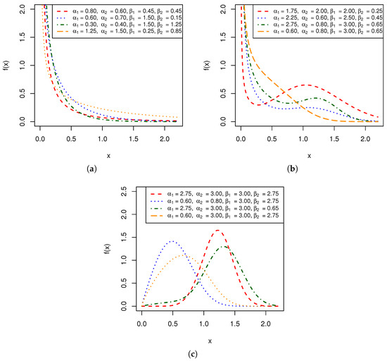
Figure 1. Different shapes of the PDF of the AGG distribution for different values of the model parameters. (a) Decreasing. (b) Non-monotonic. (c) Unimodal.

Figure 2. Different shapes of the HRF of the AGG distribution for different values of the model parameters. (a) Decreasing. (b) Non-monotonic bathtub-shaped. (c) Increasing.

2.2. Sub-Models

The AGG distribution is flexible since it comprises various well-known sub-models. In fact, it is a generalization for the exponential, linear-exponential, Rayleigh, Weibull, and gamma distributions. Moreover, it is a generalization of the additive gamma distribution and the additive Weibull distribution. The latter probability distribution belongs to a family of Gurvich’s generalized family of Weibull distributions [50] (see also [51,52] in this connection), and it was initially introduced by [53]. Explicit expressions for the moments and other fundamental distributional properties were considered by [54], who discussed model parameter estimation by the maximum likelihood methodology and obtained the corresponding observed information matrix, while [55] generalized the additive Weibull distribution by exponentiating its CDF, and discussed some statistical properties of the new generalization and maximum likelihood estimation for parameters. Table 1 summarizes the sub-models of the AGG distribution.

Table 1. The sub-models of AGG distribution.

Model	Parameters	CDF
Exponential	${\beta }_1={\beta }_2=1,{\alpha }_1={\alpha }_2=1$	$1-e^{-2\left({\displaystyle \frac{x}{\lambda }}\right)}$
Rayleigh	${\beta }_1={\beta }_2=2,{\alpha }_1={\alpha }_2=1$	$1-e^{-2{\left({\displaystyle \frac{x}{\lambda }}\right)}^2}$
Weibull	${\beta }_1={\beta }_2=\beta ,{\alpha }_1={\alpha }_2=1$	$1-e^{-2{\left({\displaystyle \frac{x}{\lambda }}\right)}^{\beta }}$
Linear exponential	${\beta }_1=2,{\beta }_2=1,{\alpha }_1={\alpha }_2=1$	$1-e^{-\left({\displaystyle \frac{x}{\lambda }}\right)-{\left({\displaystyle \frac{x}{\lambda }}\right)}^2}$
Additive Weibull	${\beta }_1\ne {\beta }_2,{\alpha }_1={\alpha }_2=1$	$1-e^{-{\left({\displaystyle \frac{x}{\lambda }}\right)}^{{\beta }_1}-{\left({\displaystyle \frac{x}{\lambda }}\right)}^{{\beta }_2}}$
Additive Gamma	${\beta }_1={\beta }_2=1,{\alpha }_1\ne {\alpha }_2$	$1-{\displaystyle \frac{\mathrm{\Gamma }\left({\alpha }_1,\left[\frac{x}{{\lambda }_1}\right]\right)}{\mathrm{\Gamma }\left({\alpha }_1\right)}}{\displaystyle \frac{\mathrm{\Gamma }\left({\alpha }_2,\left[\frac{x}{{\lambda }_2}\right]\right)}{\mathrm{\Gamma }\left({\alpha }_2\right)}}$

2.3. Statistical Properties

In this subsection, key statistical properties are obtained, namely, the moments and the quantiles.

2.3.1. Moments

To obtain the rth moment of the AGG distribution, one must obtain the rth moment of the GG distribution and apply the Fubini–Tonelli theorem when interchanging the order of integration and infinite summation; see [56,57] for this connection. The rth moment of the GG distribution is given by

$$E_i\left(X^r\right)={\mu }_r\left({\alpha }_i,{\beta }_i,{\lambda }_i\right)={\int }_0^{\infty }{x}^r{f}_i\left(x\right)dx={\lambda }_i^r{\displaystyle \frac{\mathrm{\Gamma }\left(\frac{r}{{\beta }_i}+{\alpha }_i\right)}{\mathrm{\Gamma }\left({\alpha }_i\right)}}$$

(9)

According to [58], it is straightforward to show that

$$\begin{array}{c}\hfill \begin{array}{c}\hfill \mathrm{\Gamma }\left({\alpha }_i\right)=\mathrm{\Gamma }\left({\alpha }_i,{\left[{\displaystyle \frac{x}{{\lambda }_i}}\right]}^{{\beta }_i}\right)+\sum _{k=0}^{\infty }{\displaystyle \frac{{\left(-1\right)}^k}{\mathrm{\Gamma }\left(k+1\right)\left({\alpha }_i+k\right){\lambda }_i^{{\beta }_i({\alpha }_i+k)}}}{x}^{{\beta }_i({\alpha }_i+k)}.\end{array}\end{array}$$

Hence,

$$\begin{array}{c}\hfill \begin{array}{cc}\hfill {\int }_0^{\infty }{x}^r{f}_1\left(x\right)[1-F_2\left(x\right)]& ={\int }_0^{\infty }{x}^r{f}_1\left(x\right){\displaystyle \frac{\mathrm{\Gamma }\left({\alpha }_2,{\left[\frac{x}{{\lambda }_2}\right]}^{{\beta }_2}\right)}{\mathrm{\Gamma }\left({\alpha }_2\right)}}\hfill \\ \hfill & ={\int }_0^{\infty }{x}^r{f}_1\left(x\right)\left[1-{\displaystyle \frac{1}{\mathrm{\Gamma }\left({\alpha }_2\right)}}\sum _{k=0}^{\infty }{\displaystyle \frac{{\left(-1\right)}^k}{\mathrm{\Gamma }\left(k+1\right)\left({\alpha }_2+k\right){\lambda }_2^{{\beta }_2({\alpha }_2+k)}}}{x}^{{\beta }_2({\alpha }_2+k)}\right]dx\hfill \\ & ={\mu }_r\left({\alpha }_1,{\beta }_1,{\lambda }_1\right)-\hfill \\ \hfill & {\displaystyle \frac{1}{\mathrm{\Gamma }\left({\alpha }_2\right)}}\sum _{k=0}^{\infty }{\displaystyle \frac{{\left(-1\right)}^k}{\mathrm{\Gamma }\left(k+1\right)\left({\alpha }_2+k\right){\lambda }_2^{{\beta }_2({\alpha }_2+k)}}}{\mu }_{r+{\beta }_2({\alpha }_2+k)}\left({\alpha }_1,{\beta }_1,{\lambda }_1\right).\hfill \end{array}\end{array}$$

Thus, the rth moment of the AGG distribution is given by

$$\begin{array}{cc}\hfill E_i\left(X^r\right)& ={\mu }_r\left({\alpha }_1,{\beta }_1,{\lambda }_1\right)+{\mu }_r\left({\alpha }_2,{\beta }_2,{\lambda }_2\right)\hfill \\ \hfill & -\left[{\displaystyle \frac{1}{\mathrm{\Gamma }\left({\alpha }_2\right)}}\sum _{k=0}^{\infty }{\displaystyle \frac{{\left(-1\right)}^k}{\mathrm{\Gamma }\left(k+1\right)\left({\alpha }_2+k\right){\lambda }_2^{{\beta }_2\left({\alpha }_2+k\right)}}}{\mu }_{r+{\beta }_2\left({\alpha }_2+k\right)}\left({\alpha }_1,{\beta }_1,{\lambda }_1\right)\right.\hfill \\ \hfill & +\left.{\displaystyle \frac{1}{\mathrm{\Gamma }\left({\alpha }_1\right)}}\sum _{k=0}^{\infty }{\displaystyle \frac{{\left(-1\right)}^k}{\mathrm{\Gamma }\left(k+1\right)\left({\alpha }_1+k\right){\lambda }_1^{{\beta }_1\left({\alpha }_1+k\right)}}}{\mu }_{r+{\beta }_1\left({\alpha }_1+k\right)}\left({\alpha }_2,{\beta }_2,{\lambda }_2\right)\right]\hfill \end{array}$$

2.3.2. Quantiles

In the statistical literature, q-quantiles are values that split sorted data or a probability distribution into q parts. They are the general form of quartiles ($q=4$), deciles ($q=10$), and percentiles ($q=100$). They have various applications, such as establishing a goodness-of-fit visualization device called the quantile–quantile (Q-Q) plot. Moreover, they are used to simulate random variates from the underlying probability model. The q-quantile, denoted by $x_q$, is obtained by solving a nonlinear equation $h\left(x_q\right)=0$, such that

$$h\left(x_q\right)=\mathrm{\Gamma }\left({\alpha }_1\right)\mathrm{\Gamma }\left({\alpha }_2\right)\left(1-q\right)-\mathrm{\Gamma }\left({\alpha }_1,{\left[{\displaystyle \frac{x_q}{{\lambda }_1}}\right]}^{{\beta }_1}\right)\mathrm{\Gamma }\left({\alpha }_2,{\left[{\displaystyle \frac{x_q}{{\lambda }_2}}\right]}^{{\beta }_2}\right)$$

Since $x_q$ cannot be obtained directly, one can use Newton’s method [59] to solve $h\left(x_q\right)=0$ as follows. Given an initial value $x_q^{\left(0\right)}$, we iterate

$$\begin{array}{c}\hfill x_q^{\left(k+1\right)}=x_q^{\left(k\right)}-{\displaystyle \frac{\mathrm{\Gamma }\left({\alpha }_1\right)\mathrm{\Gamma }\left({\alpha }_2\right)\left(1-q\right)-\mathrm{\Gamma }\left({\alpha }_1,{\left[\frac{x_q^{\left(k\right)}}{{\lambda }_1}\right]}^{{\beta }_1}\right)\mathrm{\Gamma }\left({\alpha }_2,{\left[\frac{x_q^{\left(k\right)}}{{\lambda }_2}\right]}^{{\beta }_2}\right)}{\mathrm{\Gamma }\left({\alpha }_1\right)f_1\left(x_q^{\left(k\right)}\right)\mathrm{\Gamma }\left({\alpha }_2,{\left[\frac{x_q^{\left(k\right)}}{{\lambda }_2}\right]}^{{\beta }_2}\right)+\mathrm{\Gamma }\left({\alpha }_2\right)f_2\left(x_q^{\left(k\right)}\right)\mathrm{\Gamma }\left({\alpha }_1,{\left[\frac{x_q^{\left(k\right)}}{{\lambda }_1}\right]}^{{\beta }_1}\right)}}\end{array}$$

(10)

for $k=1,2,\dots$ such that $\left|1-{\displaystyle \frac{x_q^{\left(k\right)}}{x_q^{\left(k+1\right)}}}\right|<ϵ$, where $ϵ\to 0$. For the initial value $x_q^{\left(0\right)}$, one can consider $x_q^{\left(0\right)}=min\left(X_1,X_2\right)$ from the physical interpretation of the survival function of the AGG distribution. Moreover, since $X_i$ follows the GG distribution with shape parameters ${\alpha }_i$ and ${\beta }_i$ and a scale parameter ${\lambda }_i$, then $X_i={\lambda }_1{Z}_i^{1/{\beta }_1}$ such that $Z_i$ follows the conventional gamma distribution with a shape parameter ${\alpha }_i$ and a scale parameter equal to 1. Accordingly, $Z_i=G_i^{-1}\left(q\right)$, where $G_i^{-1}\left(·\right)$ is the inverse of the CDF of the classical gamma distribution with a shape parameter ${\alpha }_i$ and a scale parameter equal to 1. Table 2 shows the solutions of $h\left(x_q\right)=0$ assuming various values for q using Brent’s method [60] and the corresponding approximation of Newton’s method for various values of the model parameters assuming $ϵ={10}^{-2}$ without loss of generality.

Table 2. The q-quantiles assuming Brent’s method ($x_q$) and Newton’s method ($x_q^{\ast }$).

${\mathit{\alpha }}_1$	${\mathit{\alpha }}_2$	${\mathit{\beta }}_1$	${\mathit{\beta }}_2$	${\mathit{\lambda }}_1$	${\mathit{\lambda }}_2$	q	${\mathit{x}}_{\mathit{q}}$	${\mathit{x}}_{\mathit{q}}^{\ast }$
0.9	0.9	0.8	0.95	0.5	1.5	0.1	0.015117	0.015117
0.9	0.9	0.8	0.95	0.5	1.5	0.25	0.056910	0.056892
0.9	0.9	0.8	0.95	0.5	1.5	0.5	0.178640	0.178640
0.9	0.9	0.8	0.95	0.5	1.5	0.75	0.434103	0.434099
0.9	0.9	0.8	0.95	0.5	1.5	0.9	0.824318	0.824322
1.75	2	2	1.75	2	2.5	0.1	1.389480	1.389481
1.75	2	2	1.75	2	2.5	0.25	1.728532	1.728546
1.75	2	2	1.75	2	2.5	0.5	2.218734	2.218739
1.75	2	2	1.75	2	2.5	0.75	2.784660	2.784662
1.75	2	2	1.75	2	2.5	0.9	3.336842	3.336840
2.75	3	0.85	0.65	0.5	1	0.1	0.787955	0.787956
2.75	3	0.85	0.65	0.5	1	0.25	1.031164	1.031167
2.75	3	0.85	0.65	0.5	1	0.5	1.500599	1.500619
2.75	3	0.85	0.65	0.5	1	0.75	2.209882	2.209883
2.75	3	0.85	0.65	0.5	1	0.9	3.076120	3.076110
0.8	0.8	2	1.75	2.5	4	0.1	0.409684	0.409683
0.8	0.8	2	1.75	2.5	4	0.25	0.782841	0.782841
0.8	0.8	2	1.75	2.5	4	0.5	1.361231	1.361231
0.8	0.8	2	1.75	2.5	4	0.75	2.079365	2.079387
0.8	0.8	2	1.75	2.5	4	0.9	2.812611	2.812611
0.9	3	3	2.75	3	2.5	0.1	2.473862	2.473860
0.9	3	3	2.75	3	2.5	0.25	2.649346	2.649346
0.9	3	3	2.75	3	2.5	0.5	2.956975	2.956975
0.9	3	3	2.75	3	2.5	0.75	3.342883	3.342911
0.9	3	3	2.75	3	2.5	0.9	3.721376	3.721381
2.25	2.5	2	0.65	1.5	1.5	0.1	1.293811	1.293811
2.25	2.5	2	0.65	1.5	1.5	0.25	1.581975	1.581991
2.25	2.5	2	0.65	1.5	1.5	0.5	2.008057	2.008076
2.25	2.5	2	0.65	1.5	1.5	0.75	2.502279	2.502309
2.25	2.5	2	0.65	1.5	1.5	0.9	2.984889	2.984911
1.5	0.9	3	0.85	1.5	2.5	0.1	0.449450	0.449450
1.5	0.9	3	0.85	1.5	2.5	0.25	0.767233	0.767246
1.5	0.9	3	0.85	1.5	2.5	0.5	1.220258	1.220265
1.5	0.9	3	0.85	1.5	2.5	0.75	1.632157	1.632127
1.5	0.9	3	0.85	1.5	2.5	0.9	1.969129	1.969129
0.7	0.7	2	0.75	2.5	3	0.1	0.030656	0.030671
0.7	0.7	2	0.75	2.5	3	0.25	0.167366	0.167368
0.7	0.7	2	0.75	2.5	3	0.5	0.590651	0.590658
0.7	0.7	2	0.75	2.5	3	0.75	1.323657	1.323642
0.7	0.7	2	0.75	2.5	3	0.9	2.165974	2.165982
1.75	0.4	0.45	0.55	1.7	1.6	0.1	0.124859	0.124858
1.75	0.4	0.45	0.55	1.7	1.6	0.25	0.206257	0.206259
1.75	0.4	0.45	0.55	1.7	1.6	0.5	0.474718	0.474710
1.75	0.4	0.45	0.55	1.7	1.6	0.75	1.226658	1.226658
1.75	0.4	0.45	0.55	1.7	1.6	0.9	2.801610	2.801599

2.3.3. The Mean Residual Lifetime

The mean residual lifetime (MRLT) is a concept in reliability and survival analyses that describes the expected remaining lifetime of a system, component, object, or species given that it has survived up to a specific time threshold. Under the assumption that the mean residual lifetime (MRLT) model for the failure time is conditioned on the failure of interest, a recent study by [61] considered a mixture regression model for competing risks data, where the logistic regression model is specified for the marginal probabilities of the failure types. Based on Equations (3) and (5), the MRLT is given by

$$m(t;\mathit{\theta })=E(X-T|X>t)={\displaystyle \frac{1}{S(t;\mathit{\theta })}}{\int }_t^{\infty }(x-t)f(t;\mathit{\theta })dx.$$

(11)

The behavior of the MRLT can be evaluated by rewriting Equation (11) as follows:

$$m(t;\mathit{\theta })={\int }_0^{\infty }exp\left(-{\int }_t^{x+t}h(\tau ;\mathit{\theta })d\tau \right)dx,$$

(12)

where $h(x;\mathit{\theta })$ is the HRF (6); see [62]. Figure 3 shows the shape of the MRLT (12) for different values of the model parameters $\mathit{\theta }$. The latter figure shows that the MRLT behaves oppositely to the HRF; for example, if the HRF is increasing, the MRLT is decreasing.

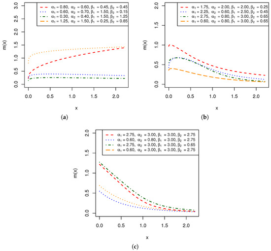
Figure 3. Different shapes of the MRLT of the AGG distribution for different values of the model parameters. (a) Increasing. (b) Non-monotonic upside-down bathtub-shaped. (c) Decreasing.

3. Estimation Procedures

This section is dedicated to discussing seven estimation methods for the parameters of the AGG distribution. It is essential to mention that it is assumed that all estimators from these methods exist and are unique. Mathematically proving the existence and uniqueness of estimators in the case of the AGG distribution is an open problem, and it is beyond the scope of this study.

3.1. Maximum Likelihood Method

The ML estimation is a statistical inference framework in which model parameters are estimated by maximizing the log-likelihood function with respect to the unknown parameters. It is a widely used approach in many fields. Suppose that $\mathbf{x}=(x_1,x_2,\dots ,x_n)$ is an observed random sample of size n from the GG risk model. Also, suppose that for each i, $I({\delta }_i=1)$ is an indicator function which indicates that the cause of failure is the first cause, while $I({\delta }_i=2)$ indicates that the cause of failure is the second risk factor. Finally, assume $I({\delta }_i=\ast )$ indicates that the cause of failure is either the first cause or the second cause, but which cause leads to failure is unknown (i.e., unknown cause of failure). Hence, we are under the assumption that some causes are known, and others are unknown. Therefore, in summary, we have the following types of observations: $(x_i,1),(x_i,2)$, and $(x_i,\ast )$. The likelihood contributions from the observations are, respectively, $f_1\left(xi\right)S_2\left(xi\right), f_2\left(x_i\right)S_1\left(x_i\right)$, and $f_1\left(x_i\right)S_2\left(x_i\right)+f_2\left(x_i\right)S_1\left(x_i\right)$. The likelihood function is given by

$$\begin{array}{c}\hfill \mathcal{l}\left(\mathit{\theta }|\mathbf{x}\right)=\prod _{i=1}^n{\left[f_1\left(x_i\right)S_2\left(x_i\right)\right]}^{I({\delta }_i=1)}{\left[f_1\left(x_i\right)S_2\left(x_i\right)\right]}^{I({\delta }_i=2)}{\left[f_1\left(x_i\right)S_2\left(x_i\right)+f_2\left(x_i\right)S_1\left(x_i\right)\right]}^{I({\delta }_i=\ast )}\end{array}$$

(13)

such that

$$I\left({\delta }_i=1\right)=\left\{\begin{array}{cc}1& \mathrm{if} {\delta }_i=1;\\ 0& \mathrm{if} {\delta }_i\ne 1\end{array}\right.$$

$$I\left({\delta }_i=2\right)=\left\{\begin{array}{cc}1& \mathrm{if} {\delta }_i=2;\\ 0& \mathrm{if} {\delta }_i\ne 2\end{array}\right.$$

and

$$I\left({\delta }_i=\ast \right)=\left\{\begin{array}{cc}1& \mathrm{if} {\delta }_i=\ast ;\\ 0& \mathrm{if} {\delta }_i\ne \ast \end{array}\right.$$

However, we consider the case where all causes of failure are unknown for this method and henceforth. Thus, the corresponding MLEs of $\mathit{\theta }$, say, ${\widehat{\mathit{\theta }}}^{\mathrm{MLE}}=({\widehat{\alpha }}_1^{\mathrm{MLE}},{\widehat{\alpha }}_2^{\mathrm{MLE}},{\widehat{\beta }}_1^{\mathrm{MLE}},{\widehat{\beta }}_2^{\mathrm{MLE}},{\widehat{\lambda }}_1^{\mathrm{MLE}},{\widehat{\lambda }}_2^{\mathrm{MLE}})$, are obtained by maximizing the following objective:

$$\begin{array}{c}\hfill \mathcal{l}\left(\mathit{\theta }|\mathbf{x}\right)\propto \sum _{i=1}^{n}log\left[f_1\left(x_i\right)S_2\left(x_i\right)+f_2\left(x_i\right)S_1\left(x_i\right)\right]\end{array}$$

(14)

where $\mathcal{l}\left(\mathit{\theta }\right|\mathbf{x})$ is the log-likelihood function without the normalized constant term. $f_j$ and $S_j$ are given, respectively, by Equations (1) and (2), where $j=1,2$. The first partial derivatives of Equation (14) with respect to ${\alpha }_j,{\beta }_j$ and ${\lambda }_j,$ are

$$\begin{array}{c}\hfill \begin{array}{cc}\hfill {\displaystyle \frac{\partial \mathcal{l}}{\partial {\alpha }_j}}& =\sum _{i=1}^n{\displaystyle \frac{1}{f\left(x_i\right)}}\{f_1\left(x_i\right)S_{3-j}\left(x_i\right)\left[{\beta }_{j}ln\left({\displaystyle \frac{x_i}{\lambda }}\right)-\psi \left({\alpha }_j\right)\right]\hfill \\ \hfill & +f_{3-j}\left(x_i\right)[{\displaystyle \frac{1}{\mathrm{\Gamma }\left({\alpha }_j\right)}}{\int }_{{\left({\displaystyle \frac{x_i}{{\lambda }_j}}\right)}^{{\beta }_j}}^{\infty }{w}^{{\alpha }_j-1}{e}^{-w}lnwdw-\psi \left({\alpha }_j\right)S_j\left(x_i\right)]\}\hfill \\ \\ \hfill {\displaystyle \frac{\partial \mathcal{l}}{\partial {\beta }_j}}& =\sum _{i=1}^n{\displaystyle \frac{1}{f\left(x_i\right)}}\{f_1\left(x_i\right)S_{3-j}\left(x_i\right)\left[{\displaystyle \frac{1}{{\beta }_j}}-{\left({\displaystyle \frac{x_i}{{\lambda }_j}}\right)}^{{\beta }_j}ln\left({\displaystyle \frac{x_i}{{\lambda }_j}}\right)+{\alpha }_{j}ln\left({\displaystyle \frac{x_i}{{\lambda }_j}}\right)\right]\hfill \\ \hfill & +f_j\left(x_i\right)f_{3-j}\left(x_i\right)\left({\displaystyle \frac{x_i}{{\beta }_j}}\right)ln\left({\displaystyle \frac{x_i}{{\lambda }_j}}\right)\}\hfill \\ \\ \hfill {\displaystyle \frac{\partial \mathcal{l}}{\partial {\lambda }_j}}& =\sum _{i=1}^n{\displaystyle \frac{1}{f\left(x_i\right)}}\left\{f_j\left(x_i\right)S_{3-j}\left(x_i\right)\left[{\displaystyle \frac{{\beta }_j{x}_i^{{\beta }_j}}{{\lambda }_j^{{\beta }_j+1}}}-{\displaystyle \frac{{\alpha }_j{\beta }_j}{{\lambda }_j}}\right]+f_j\left(x_i\right)f_{3-j}\left(x_i\right)\left({\displaystyle \frac{x_i}{{\lambda }_j}}\right)\right\}\hfill \end{array}\end{array}$$

where $j=1,2$ and $\psi \left(\alpha \right)={\displaystyle \frac{d}{d\alpha }}ln\mathrm{\Gamma }\left(\alpha \right)={\displaystyle \frac{{\mathrm{\Gamma }}^{\prime }\left(\alpha \right)}{\mathrm{\Gamma }\left(\alpha \right)}}$ is the digamma function, respectively. The normal equations are obtained by equating these partial derivatives to 0. Since the resulting equations are nonlinear, the MLEs are obtained numerically using an appropriate optimization approach, assuming the existence and uniqueness of these estimators.

3.2. Maximum Product of Spacing Estimation

Another estimation approach based on maximization is the maximum product of spacings (MPS) framework, which yields MPS estimates (MPSEs). These estimators compete with maximum likelihood estimators (MLEs) in terms of efficiency and asymptotic performance, as demonstrated in [63,64,65,66]. However, ties complicate MPSE computation, as the conventional method cannot be applied directly. To address this issue, ref. [67] introduced a generalized maximum product of spacings method. The idea of the method is to maximize the geometric mean of the differences between the distribution function values at adjacent ordered points. Suppose that ${\mathbf{x}}^{\ast }=(x_{1:n},x_{2:n},\dots ,x_{n:n})$ are the corresponding observed order statistics based on a random sample of size n from the AGG distribution with an arbitrary CDF with model parameters $\mathit{\theta }$, say, $F(x;\mathit{\theta })$, such that $F(x_{0:n};\mathit{\theta })=0$ and $F(x_{n+1:n};\mathit{\theta })=1$. The MPSEs of $\mathit{\theta }$, say, ${\widehat{\mathit{\theta }}}^{\mathrm{MPSE}}=({\widehat{\alpha }}_1^{\mathrm{MPSE}},{\widehat{\alpha }}_2^{\mathrm{MPSE}},{\widehat{\beta }}_1^{\mathrm{MPSE}},{\widehat{\beta }}_2^{\mathrm{MPSE}},{\widehat{\lambda }}_1^{\mathrm{MPSE}},{\widehat{\lambda }}_2^{\mathrm{MPSE}})$, are acquired by maximizing

$$P(\mathit{\theta }\mid {\mathbf{x}}^{\ast })={\displaystyle \frac{1}{n+1}}\sum _{i=1}^{n+1}log{△}_i,$$

(15)

such that

$$\begin{array}{c}\left\{\begin{array}{cc}F\left(x_{1:n};\mathit{\theta }\right)\hfill & \mathrm{if} i=1\hfill \\ F\left(x_{i:n};\mathit{\theta }\right)-F\left(x_{i-1:n};\mathit{\theta }\right)\hfill & \mathrm{if} 1<i\le n\hfill \\ 1-F\left(x_{n:n};\mathit{\theta }\right)\hfill & \mathrm{if} i=n+1\hfill \end{array}\right.\hfill \end{array}.$$

The first partial derivatives of Equation (15) with respect to the model parameters are as follows:

$$\begin{array}{c}\hfill {\displaystyle \frac{\partial P}{\partial {\alpha }_j}}={\displaystyle \frac{1}{n+1}}\sum _{i=1}^{n+1}{\displaystyle \frac{B_{{\alpha }_j}{△}_i}{{△}_i}},{\displaystyle \frac{\partial P}{\partial {\beta }_j}}={\displaystyle \frac{1}{n+1}}\sum _{i=1}^{n+1}{\displaystyle \frac{B_{{\beta }_j}{△}_i}{{△}_i}},{\displaystyle \frac{\partial P}{\partial {\lambda }_j}}={\displaystyle \frac{1}{n+1}}\sum _{i=1}^{n+1}{\displaystyle \frac{B_{{\lambda }_j}{△}_i}{{△}_i}},\end{array}$$

where

$$B_{{\alpha }_j}{△}_i=\left\{\begin{array}{cc}{\tau }_{{\alpha }_j}(x_{1:n};\mathit{\theta })\hfill & \mathrm{if} i=1\hfill \\ {\tau }_{{\alpha }_j}(x_{i:n};\mathit{\theta })-{\tau }_{{\alpha }_j}(x_{i-1:n};\mathit{\theta })\hfill & \mathrm{if} 1<i\le n,\hfill \\ -{\tau }_{{\alpha }_j}(x_{n:n};\mathit{\theta })\hfill & \mathrm{if} i=n+1\hfill \end{array}\right.$$

$$B_{{\beta }_j}{△}_i=\left\{\begin{array}{cc}{\tau }_{{\beta }_j}(x_{1:n};\mathit{\theta })\hfill & \mathrm{if} i=1;\hfill \\ {\tau }_{{\beta }_j}(x_{i:n};\mathit{\theta })-{\tau }_{{\beta }_j}(x_{i-1:n};\mathit{\theta })\hfill & \mathrm{if} 1<i\le n;\hfill \\ -{\tau }_{{\beta }_j}(x_{n:n};\mathit{\theta })\hfill & \mathrm{if} i=n+1.\hfill \end{array}\right.$$

$$B_{{\lambda }_j}{△}_i=\left\{\begin{array}{cc}{\tau }_{{\lambda }_j}(x_{1:n};\mathit{\theta })\hfill & \mathrm{if} i=1\hfill \\ {\tau }_{{\lambda }_j}(x_{i:n};\mathit{\theta })-{\tau }_{{\lambda }_j}(x_{i-1:n};\mathit{\theta })\hfill & \mathrm{if} 1<i\le n.\hfill \\ -{\tau }_{{\lambda }_j}(x_{n:n};\mathit{\theta })\hfill & \mathrm{if} i=n+1\hfill \end{array}\right.,$$

such that

$${\tau }_{{\alpha }_j}(x_{i:n};\mathit{\theta })={\displaystyle \frac{\partial F(x_{i:n};\mathit{\theta })}{\partial {\alpha }_j}}=S_{3-j}\left(x_{i:n}\right)\left[\psi \left({\alpha }_j\right)S_j\left(x_{i:n}\right)-{\displaystyle \frac{1}{\mathrm{\Gamma }\left({\alpha }_j\right)}}{\int }_{{\left({\displaystyle \frac{x_{i:n}}{{\lambda }_j}}\right)}^{{\beta }_j}}^{\infty }{w}^{{\alpha }_j-1}{e}^{-w}lnwdw\right],$$

(16)

$${\tau }_{{\beta }_j}(x_{i:n};\mathit{\theta })={\displaystyle \frac{\partial F(x_{i:n};\mathit{\theta })}{\partial {\beta }_j}}={\displaystyle \frac{x_{i:n}}{{\beta }_j}}ln\left({\displaystyle \frac{x_{i:n}}{{\lambda }_j}}\right)S_{3-j}\left(x_{i:n}\right)f_j\left(x_{i:n}\right),$$

(17)

and

$${\tau }_{{\lambda }_j}(x_{i:n};\mathit{\theta })={\displaystyle \frac{\partial F(x_{i:n};\mathit{\theta })}{\partial {\lambda }_j}}={\displaystyle \frac{x_{i:n}}{{\lambda }_j}}{S}_{3-j}\left(x_{i:n}\right)f_j\left(x_{i:n}\right),$$

(18)

for $j=1,2$. Note that these expressions are frequently used in the following subsections.

3.3. Least Square Estimation

In a study by [68], LSEs were obtained for the beta distribution model parameters. Recall that $\mathbf{x}=(x_1,x_2,\dots ,x_n)$ is an observed random sample, and ${\mathbf{x}}^{\ast }=(x_{1:n},x_{2:n},\dots ,x_{n:n})$ are the corresponding observed order statistics. Thus, $F(x_{1:n};\mathit{\theta }),\dots ,F(x_{n:n};\mathit{\theta })$ are order statistics from a standard uniform distribution with expected values:

$$\mathrm{E}\left[F(x_{i:n};\mathit{\theta })\right]={\displaystyle \frac{i}{n+1}},$$

such that $i=1,\dots ,n$ [69]. The LSEs of $\mathit{\theta }$, say, ${\widehat{\mathit{\theta }}}^{\mathrm{LSE}}=({\widehat{\alpha }}_1^{\mathrm{LSE}},{\widehat{\alpha }}_2^{\mathrm{LSE}},{\widehat{\beta }}_1^{\mathrm{LSE}},{\widehat{\beta }}_2^{\mathrm{LSE}},{\widehat{\lambda }}_1^{\mathrm{LSE}},{\widehat{\lambda }}_2^{\mathrm{LSE}})$, are obtained by minimizing the following least squares objective function:

$$\begin{array}{c}\hfill S\left(\mathit{\theta }\right|{\mathbf{x}}^{\ast })=\sum _{i=1}^n{\left[F(x_{i:n};\mathit{\theta })-{\displaystyle \frac{i}{n+1}}\right]}^2\end{array}$$

(19)

The first partial derivatives of Equation (19) with respect to model parameters are given by

$$\begin{array}{c}\hfill \begin{array}{c}\hfill {\displaystyle \frac{\partial S}{\partial {\alpha }_j}}=2\sum _{i=1}^n\left[F(x_{i:n};\mathit{\theta })-{\displaystyle \frac{i}{n+1}}\right]{\tau }_{{\alpha }_j}(x_{i:n};\mathit{\theta }),\end{array}\end{array}$$

$$\begin{array}{c}\hfill {\displaystyle \frac{\partial S}{\partial {\beta }_j}}=2\sum _{i=1}^n\left[F(x_{i:n};\mathit{\theta })-{\displaystyle \frac{i}{n+1}}\right]{\tau }_{{\beta }_j}(x_{i:n};\mathit{\theta }),\end{array}$$

and

$$\begin{array}{c}\hfill {\displaystyle \frac{\partial S}{\partial {\lambda }_j}}=2\sum _{i=1}^n\left[F(x_{i:n};\mathit{\theta })-{\displaystyle \frac{i}{n+1}}\right]{\tau }_{{\lambda }_j}(x_{i:n};\mathit{\theta }),\end{array}$$

where $j=1,2$ and ${\tau }_{{\alpha }_j}(x_{i:n};\mathit{\theta }),{\tau }_{{\beta }_j}(x_{i:n};\mathit{\theta })$ and ${\tau }_{{\lambda }_j}(x_{i:n};\mathit{\theta })$ are defined by (16)–(18).

3.4. Weighted Least Square Estimation

Alongside the LSEs, ref. [68] considered WLSEs for the beta distribution parameters. Recall that $x_{1:n},x_{2:n},\dots x_{n:n}$ are the observed order statistics. From [69], it is known that

$$Var\left[F\left(x_{i:n}\right)\right]={\displaystyle \frac{i(n-i+1)}{{(n+1)}^2(n+2)}},$$

since $F\left(x_{1:n}\right),F\left(x_{2:n}\right),\dots ,F\left(x_{n:n}\right)$ are order statistics from a standard uniform distribution. The WLSEs of ${\widehat{\mathit{\theta }}}^{\mathrm{WLSE}}=({\widehat{\alpha }}_1^{\mathrm{WLSE}},{\widehat{\alpha }}_2^{\mathrm{WLSE}},{\widehat{\beta }}_1^{\mathrm{WLSE}},{\widehat{\beta }}_2^{\mathrm{WLSE}},{\widehat{\lambda }}_1^{\mathrm{WLSE}},{\widehat{\lambda }}_2^{\mathrm{WLSE}})$ are computed after minimizing the objective function:

$$\begin{array}{c}\hfill S_w\left(\mathit{\theta }{\mathbf{x}}^{\ast }\right)=\sum _{i=1}^n{w}_{i:n}[F(x_{i:n};\mathit{\theta })-{\displaystyle \frac{i}{n+1}}{]}^2\end{array}$$

(20)

where $w_{1:n},w_{2:n},\dots ,w_{n:n}$ are the weights, such that $w_{i:n}={\left\{Var\left[F\left(x_{i:n}\right)\right]\right\}}^{-1}$. The first partial derivatives of Equation (20) with respect to model parameters are

$$\begin{array}{cc}\hfill {\displaystyle \frac{\partial S_w}{\partial {\alpha }_j}}& =2\sum _{i=1}^n{w}_{i:n}[F(x_{i:n};\mathit{\theta })-{\displaystyle \frac{i}{n+1}}]{\tau }_{{\alpha }_j}(x_{i:n};\mathit{\theta }),\hfill \end{array}$$

$$\begin{array}{cc}\hfill {\displaystyle \frac{\partial S_w}{\partial {\beta }_j}}& =2\sum _{i=1}^n{w}_{i:n}[F(x_{i:n};\mathit{\theta })-{\displaystyle \frac{i}{n+1}}]{\tau }_{{\beta }_j}(x_{i:n};\mathit{\theta }),\hfill \end{array}$$

and

$$\begin{array}{cc}\hfill {\displaystyle \frac{\partial S_w}{\partial {\lambda }_j}}& =2\sum _{i=1}^n{w}_{i:n}[F(x_{i:n};\mathit{\theta })-{\displaystyle \frac{i}{n+1}}]{\tau }_{{\lambda }_j}(x_{i:n};\mathit{\theta }),\hfill \end{array}$$

for $j=1,2$.

3.5. Cramér–von Mises Estimation

Some estimators can be acquired under a minimum-distance framework in the statistical literature. Under this framework, the difference between an empirical distribution function and the hypothesized model distribution function is minimized. The first estimation method is per Cramér–von Mises statistic, which is used for the goodness-of-fit test. Recall that the observed order statistics ${\mathbf{x}}^{\ast }$ of a random sample $\mathbf{x}$ of size n with CDF $F\left(x_{i:n}\right)$, the CVMEs of $\mathit{\theta }$, say, ${\widehat{\mathit{\theta }}}^{\mathrm{CVME}}=({\widehat{\alpha }}_1^{\mathrm{CVME}},{\widehat{\alpha }}_2^{\mathrm{CVME}},{\widehat{\beta }}_1^{\mathrm{CVME}},{\widehat{\beta }}_2^{\mathrm{CVME}},{\widehat{\lambda }}_1^{\mathrm{CVME}},{\widehat{\lambda }}_2^{\mathrm{CVME}})$, are calculated by minimizing

$$C\left(\mathit{\theta }\right|{\mathbf{x}}^{\ast })={\displaystyle \frac{1}{12n}}+\sum _{i=1}^n{\left[F(x_{i:n};\mathit{\theta })-{\displaystyle \frac{2i-1}{2n}}\right]}^2.$$

(21)

The first partial derivative of Equation (21) with respect to model parameters, are given by

$$\begin{array}{cc}\hfill {\displaystyle \frac{\partial C}{\partial {\alpha }_j}}& =-2\sum _{i=1}^n\left[F(x_{i:n};\mathit{\theta })-{\displaystyle \frac{2i-1}{2n}}\right]{\tau }_{{\alpha }_j}(x_{i:n};\mathit{\theta }),\hfill \end{array}$$

$$\begin{array}{cc}\hfill {\displaystyle \frac{\partial C}{\partial {\beta }_j}}& =-2\sum _{i=1}^n\left[F(x_{i:n};\mathit{\theta })-{\displaystyle \frac{2i-1}{2n}}\right]{\tau }_{{\beta }_j}(x_{i:n};\mathit{\theta }),\hfill \end{array}$$

and

$$\begin{array}{cc}\hfill {\displaystyle \frac{\partial C}{\partial {\lambda }_j}}& =-2\sum _{i=1}^n\left[F(x_{i:n};\mathit{\theta })-{\displaystyle \frac{2i-1}{2n}}\right]{\tau }_{{\lambda }_j}(x_{i:n};\mathit{\theta }),\hfill \end{array}$$

for $j=1,2$.

3.6. Anderson–Darling Estimation

Another minimum-distance estimation method is the Anderson–Darling method. This approach may provide robust and efficient estimators; see [70]. Recall that the observed order statistics ${\mathbf{x}}^{\ast }$ of a random sample $\mathbf{x}$ of size n with CDF $F\left(x_{i:n}\right)$, the ADEs of $\mathit{\theta }$, say, ${\widehat{\mathit{\theta }}}^{\mathrm{ADE}}=({\widehat{\alpha }}_1^{\mathrm{ADE}},{\widehat{\alpha }}_2^{\mathrm{ADE}},{\widehat{\beta }}_1^{\mathrm{ADE}},{\widehat{\beta }}_2^{\mathrm{ADE}},{\widehat{\lambda }}_1^{\mathrm{ADE}},{\widehat{\lambda }}_2^{\mathrm{ADE}})$, are obtained by minimizing the following objective function:

$$\begin{array}{cc}\hfill A\left(\mathit{\theta }\right|{\mathbf{x}}^{\ast })& =-n-{\displaystyle \frac{1}{n}}\sum _{i=1}^n(2i-1)\{log\left[F(x_{i:n};\mathit{\theta })\right]+log\left[S(x_{n-i+1:n};\mathit{\theta })\right]\}.\hfill \end{array}$$

(22)

The first partial derivative of Equation (22) with respect to model parameters are given by

$$\begin{array}{cc}\hfill {\displaystyle \frac{\partial A}{\partial {\alpha }_j}}& ={\displaystyle \frac{1}{n}}\sum _{i=1}^n(2i-1)\{{\tau }_{{\alpha }_j}(x_{i:n};\mathit{\theta }){\left[F\right(x_{i:n};\mathit{\theta }\left)\right]}^{-1}+{\tau }_{{\alpha }_j}(x_{i:n};\mathit{\theta }){\left[S(x_{n-i+1:n};\mathit{\theta })\right]}^{-1}\},\hfill \end{array}$$

$$\begin{array}{cc}\hfill {\displaystyle \frac{\partial A}{\partial {\beta }_j}}& ={\displaystyle \frac{1}{n}}\sum _{i=1}^n(2i-1)\{{\tau }_{{\beta }_j}(x_{i:n};\mathit{\theta }){\left[F(x_{i:n};\mathit{\theta })\right]}^{-1}+{\tau }_{{\beta }_j}(x_{i:n};\mathit{\theta }){\left[S(x_{n-i+1:n};\mathit{\theta })\right]}^{-1}\},\hfill \end{array}$$

and

$$\begin{array}{cc}\hfill {\displaystyle \frac{\partial A}{\partial {\lambda }_j}}& ={\displaystyle \frac{1}{n}}\sum _{i=1}^n(2i-1)\{{\tau }_{{\lambda }_j}(x_{i:n};\mathit{\theta }){\left[F(x_{i:n};\mathit{\theta })\right]}^{-1}+{\tau }_{{\lambda }_j}(x_{i:n};\mathit{\theta }){\left[S(x_{n-i+1:n};\mathit{\theta })\right]}^{-1}\},\hfill \end{array}$$

for $j=1,2$.

3.7. Right-Tailed Anderson–Darling Estimation

Another version of the Anderson–Darling-based estimation method is the right-tailed Anderson–Darling method. Based on the observed order statistics ${\mathbf{x}}^{\ast }$ with CDF $F\left(x_{i:n}\right)$, the RADEs of $\mathit{\theta }$, say, ${\widehat{\mathit{\theta }}}^{\mathrm{RADE}}=({\widehat{\alpha }}_1^{\mathrm{RADE}},{\widehat{\alpha }}_2^{\mathrm{RADE}},{\widehat{\beta }}_1^{\mathrm{RADE}},{\widehat{\beta }}_2^{\mathrm{RADE}},{\widehat{\lambda }}_1^{\mathrm{RADE}},{\widehat{\lambda }}_2^{\mathrm{RADE}})$, are computed after minimizing the following objective function:

$$\begin{array}{c}\hfill \begin{array}{cc}\hfill R_A(\mathit{\theta }\mid \underline{x})& ={\displaystyle \frac{n}{2}}-{\displaystyle \frac{1}{n}}\sum _{i=1}^n(2i-1)log\left[S(x_{n-i+1:n};\mathit{\theta })\right]-2\sum _{i=1}^{n}F(x_{i:n};\mathit{\theta }).\hfill \end{array}\end{array}$$

(23)

The first partial derivative of Equation (23) with respect to model parameters are given by

$$\begin{array}{c}\hfill {\displaystyle \frac{\partial R_A}{\partial {\alpha }_j}}={\displaystyle \frac{1}{n}}\sum _{i=1}^n(2i-1){\tau }_{{\alpha }_j}(x_{n-i+1:n};\mathit{\theta }){\left[S(x_{n-i+1:n};\mathit{\theta })\right]}^{-1}-2\sum _{i=1}^n{\tau }_{{\alpha }_j}(x_{i:n};\mathit{\theta }),\end{array}$$

$$\begin{array}{c}\hfill {\displaystyle \frac{\partial R_A}{\partial {\beta }_j}}=-{\displaystyle \frac{1}{n}}\sum _{i=1}^n(2i-1){\tau }_{{\beta }_j}(x_{n-i+1:n};\mathit{\theta }){\left[S(x_{n-i+1:n};\mathit{\theta })\right]}^{-1}-2\sum _{i=1}^n{\tau }_{{\beta }_j}(x_{i:n};\mathit{\theta }),\end{array}$$

and

$$\begin{array}{c}\hfill {\displaystyle \frac{\partial R_A}{\partial {\lambda }_j}}=-{\displaystyle \frac{1}{n}}\sum _{i=1}^n(2i-1){\tau }_{{\lambda }_j}(x_{n-i+1:n};\mathit{\theta }){\left[S(x_{n-i+1:n};\mathit{\theta })\right]}^{-1}-2\sum _{i=1}^n{\tau }_{{\lambda }_j}(x_{i:n};\mathit{\theta }),\end{array}$$

for $j=1,2$.

In principle, MLEs and MPSEs are generally preferred because of their asymptotic efficiency. However, for complex survival models, their performance may deteriorate when the likelihood surface is flat, multimodal, or poorly conditioned, leading to convergence failures or unstable estimates, especially in small samples. Moreover, MLEs are sensitive to data contamination and outliers. To overcome these limitations, several alternative estimators are considered in this study. Minimum-distance estimators, such as ADEs, RADEs, and CVMEs, provide robustness by assigning different weights across the distribution. ADEs and RADEs emphasize the tails, which are particularly important in reliability and survival applications, whereas CVMEs offer a more balanced fit across the entire range. Although LSEs and WLSEs are not asymptotically efficient, they may yield stable results when likelihood-based estimators become unreliable. Accordingly, this study adopts a multi-method estimation strategy in which MLEs and MPSEs serve as the primary estimators, while the remaining procedures act as complementary approaches to improve robustness and ensure reliable inference under various data conditions.

4. Monte Carlo Simulation Outcomes

A comprehensive Monte Carlo simulation analysis is conducted to numerically analyze and compare the efficacy of the proposed estimators under different combinations of sample size n and different parameters values of ${\alpha }_1,{\alpha }_2,{\beta }_1,{\beta }_2,{\lambda }_1,{\lambda }_2$ where the parameters ${\alpha }_1,{\alpha }_2,{\beta }_1$, and ${\beta }_2$ affect the shape of the distribution while the scale parameters ${\lambda }_1$ and ${\lambda }_2$ control the spread of data, stretching the distribution along the x-axis rather than changing its fundamental shape which is basically controlled by the parameter shape. The simulation results are categorized into two sections: the first section assesses the efficiency of estimators, while the second section focuses on goodness-of-fit analysis for each estimation method. In the simulation, the sample size is designated as $n=25,50,100,250,500$; moreover, the parameter values were set as ${\alpha }_1=0.4, 1.2, 2,{\alpha }_2=0.8, 1.6, 2.4, {\beta }_1=0.4, 1.2, 2$, and ${\beta }_2=2,0.8, 1.6, 2.4$ with the scale parameters maintained at ${\lambda }_1={\lambda }_2=1$ without loss of generality. The simulation outcomes are based on $N=1000$ simulation iterations. All numerical results were obtained using RStudio 2024.12.1 [71], an integrated development environment (IDE) for R 4.4.3 [72], a language and environment designed for statistical computing, visualization, and analysis. Due to its versatility, R includes numerous built-in functions for optimization, in addition to a wide range of contributed packages. One such package is nloptr 2.2.1, which serves as an R interface to NLopt 2.10.0, a free and open-source library for nonlinear optimization. NLopt provides a unified interface to various freely available optimization routines, as well as original implementations of several algorithms [73]. Among these is the Bound Optimization by Quadratic Approximation (BOBYQA) algorithm [74], which demonstrated strong performance in obtaining the estimators.

Each estimation method was implemented using numerical optimization via the BOBYQA algorithm. We determine the stopping criteria when the relative change in the calculated optimized objects from one iteration to the next is less than ${10}^{-6}$, or when the maximum number of function evaluations ${10}^4$ is reached. The initial parameter values were obtained using uniform sampling within $\pm 10\%$ of the true parameters for each simulation run. For any of the seven estimation objects, if a failure to converge was detected (e.g., returning infinite values or reaching the maximum number of function evaluations), the optimization was repeated using a newly generated initial value until the convergence criteria were met. The estimation is ensured to be stable across all simulation runs due to adaptive re-initialization, resulting in negligible final non-convergence rates.

To acquire random samples from the underlying model, the following steps are implemented:

• Generate two independent random samples of size n for each cause of failure, i.e., $X_{11},X_{12},\dots ,X_{1n}$ represent a random sample from $\mathrm{GG}({\alpha }_1,{\beta }_1,{\lambda }_1)$ (failure #1) and $X_{21},X_{22},\dots ,X_{2n}$ form a random sample from $\mathrm{GG}({\alpha }_2,{\beta }_2,{\lambda }_2)$.
• Set $X_i=min(X_{1i},X_{2i})$ for all $i=1,\dots ,n$ to obtain a random sample from the AGG distribution.

Using the specified simulation settings and procedures described above, 1000 random samples were generated, and the model parameters were estimated using the seven previously discussed methods. As some comparison metrics yielded disproportionately large values, min–max normalization was applied to scale all results between 0 and 1. It is important to note that lower values indicate better performance; thus, an estimation method with metrics closer to 0 is considered superior to its counterparts.

4.1. Estimation Efficiency

The root mean square error (RMSE) is a common metric for assessing the average magnitude of errors between estimated values and actual values. This evaluation is crucial for determining the performance of estimators across various statistical applications. In this study, RMSE is used to compare estimator performance under varying parameter settings. The simulated RMSE is obtained for each estimator as

$$RMSE\left(\widehat{\theta }\right)=\sqrt{{\displaystyle \frac{1}{N}}\sum _{i=1}^N{({\widehat{\theta }}_i-\theta )}^2}$$

where ${\widehat{\theta }}_i$ is the point estimator of $\theta$ on simulation run i. Table 3, Table 4 and Table 5 include the estimated RMSEs for three cases of parameters selected from simulation results. For a complete visual summary, Figure 4, Figure 5, Figure 6 and Figure 7 illustrate the efficiency of the estimation and provide numerous patterns in RMSE values related to various estimation methods in differing values of parameters and sample sizes. For clarification, Figure 4 is a heatmap that displays the simulated RMSE of the estimator ${\alpha }_1$ across the seven estimation methods and different sample sizes for all combinations of the parameters ${\alpha }_2=0.8, 1.6, 2.4, {\beta }_1=0.4, 1.2, 2$, and ${\beta }_2=2, 0.8, 1.6, 2.4$; more green is associated with lower values of RMSE. The outcomes of this part of the simulation study are discussed as follows:

Table 3. Simulation results based on parameters $({\alpha }_1=0.4, {\alpha }_2=0.8, {\beta }_1=0.4, {\beta }_2=0.8)$.

Method	n	RMSE (${\widehat{\mathit{\alpha }}}_1$)	RMSE (${\widehat{\mathit{\alpha }}}_2$)	RMSE (${\widehat{\mathit{\beta }}}_1$)	RMSE (${\widehat{\mathit{\beta }}}_2$)	${\mathit{D}}_{\mathbf{max}}$	${\mathit{D}}_{\mathbf{abs}}$
	25	0.8004	1.8465	1.0632	3.0372	0.1001	0.0555
	50	0.7255	1.5829	0.9164	1.8095	0.0701	0.0387
AD	100	0.5775	1.4435	0.6736	1.4870	0.0504	0.0276
	250	0.5258	1.2486	0.4989	0.7479	0.0319	0.0173
	500	0.3529	1.0473	0.3469	0.4466	0.0227	0.0123
	25	0.7272	1.7582	0.9093	3.2716	0.1053	0.0568
	50	0.6272	1.1935	0.5935	1.4701	0.0732	0.0396
CVM	100	0.5094	1.1212	0.4966	0.8281	0.0523	0.0281
	250	0.3990	0.9897	0.3706	0.6273	0.0330	0.0176
	500	0.3342	0.7915	0.2607	0.4189	0.0233	0.0125
	25	0.7353	1.6888	0.8204	1.5170	0.1030	0.0571
	50	0.6322	1.2980	0.6213	1.2496	0.0722	0.0398
LS	100	0.5075	1.2135	0.4801	0.6870	0.0519	0.0282
	250	0.3964	0.9743	0.4247	0.6180	0.0328	0.0177
	500	0.3181	0.8043	0.2843	0.4224	0.0233	0.0125
	25	1.2893	13.4726	6.8718	26.0862	0.1020	0.0555
	50	0.7202	7.6779	2.5109	28.5677	0.0701	0.0385
ML	100	0.6396	5.3765	1.6467	14.8956	0.0507	0.0275
	250	0.5149	2.2474	1.0512	3.6352	0.0320	0.0173
	500	0.4823	4.3053	0.6874	31.6124	0.0229	0.0123
	25	1.0876	3.4826	2.3837	9.0008	0.0985	0.0561
	50	0.9115	3.7267	1.8261	6.2322	0.0696	0.0391
MPS	100	0.9172	2.9276	1.5132	5.8654	0.0506	0.0279
	250	0.7614	2.2540	1.2067	1.4484	0.0320	0.0173
	500	0.6779	1.6276	0.7578	1.2795	0.0230	0.0123
	25	0.7186	1.8848	0.9392	5.3906	0.1008	0.0557
	50	0.5461	1.7886	0.6497	1.7187	0.0702	0.0390
RAD	100	0.4720	1.7475	0.4765	1.6356	0.0508	0.0277
	250	0.3665	1.4792	0.2620	0.7995	0.0324	0.0175
	500	0.2964	1.1115	0.2097	0.5984	0.0231	0.0124
	25	0.8825	1.9071	1.0907	7.5173	0.0999	0.0562
	50	0.7163	1.7317	0.7041	2.1429	0.0703	0.0391
WLS	100	0.6037	1.4053	0.5644	1.7256	0.0504	0.0277
	250	0.4394	1.2179	0.4092	0.7320	0.0320	0.0173
	500	0.3411	1.0113	0.2996	0.5195	0.0227	0.0123

Table 4. Simulation results based on parameters $({\alpha }_1=1.2, {\alpha }_2=2.4, {\beta }_1=2,{\beta }_2=2.4)$.

Method	n	RMSE (${\widehat{\mathit{\alpha }}}_1$)	RMSE (${\widehat{\mathit{\alpha }}}_2$)	RMSE (${\widehat{\mathit{\beta }}}_1$)	RMSE (${\widehat{\mathit{\beta }}}_2$)	${\mathit{D}}_{\mathbf{max}}$	${\mathit{D}}_{\mathbf{abs}}$
	25	3.8696	4.5710	2.1805	4.5376	0.0974	0.0547
	50	2.5707	3.7078	1.3933	2.9634	0.0704	0.0391
AD	100	1.9511	3.3414	1.4341	1.7588	0.0497	0.0274
	250	1.4471	2.7918	1.1828	1.4125	0.0315	0.0172
	500	1.1344	2.0176	1.2654	1.2048	0.0227	0.0125
	25	4.9484	3.6161	3.2976	4.7298	0.1055	0.0564
	50	2.6704	2.8617	1.0925	2.7295	0.0751	0.0402
CVM	100	2.0896	2.3989	0.9408	1.7942	0.0529	0.0283
	250	1.3811	1.7719	0.8335	1.4011	0.0331	0.0176
	500	0.9346	1.5126	0.8330	1.0483	0.0238	0.0128
	25	2.8903	3.5592	1.4920	2.9227	0.1020	0.0569
	50	2.4526	2.8803	1.2525	2.4264	0.0735	0.0403
LS	100	1.9228	2.3929	0.9611	1.6200	0.0523	0.0283
	250	1.3510	1.7417	0.8104	1.3004	0.0330	0.0176
	500	0.8750	1.4886	0.6773	1.0391	0.0237	0.0128
	25	12.9767	13.6384	22.9772	36.2098	0.1008	0.0557
	50	5.1360	13.0494	9.0282	30.4231	0.0714	0.0395
ML	100	3.8944	9.1857	8.0525	29.8039	0.0501	0.0277
	250	2.9975	8.9024	5.4239	18.0750	0.0316	0.0171
	500	2.5327	8.5122	5.4875	20.2460	0.0228	0.0126
	25	4.4468	8.9473	4.0642	18.5628	0.0959	0.0558
	50	3.7992	7.3898	5.6584	10.2533	0.0690	0.0394
MPS	100	3.0723	6.9549	4.3824	8.9993	0.0489	0.0276
	250	2.3901	5.7265	5.0838	8.6194	0.0313	0.0172
	500	2.0444	4.3894	4.9907	2.0108	0.0225	0.0125
	25	3.7427	4.6234	2.8798	8.1502	0.0984	0.0552
	50	2.4967	3.6922	1.2833	5.2507	0.0717	0.0396
RAD	100	1.8601	2.9919	0.9198	3.4692	0.0508	0.0278
	250	1.2236	2.4227	0.7702	2.2605	0.0324	0.0174
	500	0.7270	1.7920	1.1720	1.4842	0.0234	0.0128
	25	3.1507	5.0549	1.8745	6.9476	0.0981	0.0557
	50	2.6520	4.3485	1.4925	3.6004	0.0708	0.0395
WLSE	100	2.0614	3.7384	1.1423	7.0709	0.0502	0.0277
	250	1.4989	3.4297	1.0560	1.8824	0.0317	0.0172
	500	1.2021	2.7426	1.1971	1.3805	0.0228	0.0126

Table 5. Simulation results based on parameters $({\alpha }_1=0.4, {\alpha }_2=0.8, {\beta }_1=2,{\beta }_2=1.6)$.

Method	n	RMSE (${\widehat{\mathit{\alpha }}}_1$)	RMSE (${\widehat{\mathit{\alpha }}}_2$)	RMSE (${\widehat{\mathit{\beta }}}_1$)	RMSE (${\widehat{\mathit{\beta }}}_2$)	${\mathit{D}}_{\mathbf{max}}$	${\mathit{D}}_{\mathbf{abs}}$
	25	1.7309	4.0228	4.0926	3.3201	0.0967	0.0543
	50	1.3968	2.9716	3.0121	1.5369	0.0699	0.0391
AD	100	1.3922	2.4048	3.1197	1.0630	0.0491	0.0276
	250	0.9791	1.7021	1.7699	0.7256	0.0313	0.0174
	500	0.8660	1.2687	1.5384	0.6139	0.0225	0.0125
	25	1.5843	3.5834	3.9039	2.5510	0.1037	0.0562
	50	1.2728	2.7742	2.5347	1.5766	0.0735	0.0402
CVM	100	1.0451	2.1096	2.1793	0.8774	0.0510	0.0282
	250	0.8889	1.5001	1.6533	0.7194	0.0326	0.0178
	500	0.7076	1.2238	1.4082	0.6151	0.0234	0.0129
	25	1.5153	3.3650	2.4229	1.9504	0.1004	0.0564
	50	1.2162	2.7090	2.0835	1.3985	0.0723	0.0404
LS	100	1.0994	2.0654	1.9541	0.8095	0.0506	0.0282
	250	0.9047	1.4962	1.5503	0.6879	0.0325	0.0178
	500	0.7240	1.2337	1.3492	0.5923	0.0234	0.0129
	25	4.5246	20.0665	41.9294	25.4423	0.1006	0.0557
	50	2.9897	12.8197	26.2575	19.2926	0.0726	0.0400
ML	100	1.7359	11.4318	17.6730	11.0614	0.0499	0.0278
	250	1.9386	3.4213	11.7639	2.6453	0.0314	0.0173
	500	1.3947	2.6450	9.9168	2.5103	0.0225	0.0125
	25	1.8195	7.9617	9.4541	9.5800	0.0946	0.0549
	50	2.1119	5.2736	8.9657	4.7021	0.0698	0.0394
MPS	100	1.7908	4.2444	47.0125	4.0985	0.0491	0.0278
	250	1.8792	2.6294	9.6275	1.6218	0.0311	0.0174
	500	1.6184	2.0046	4.4688	0.9240	0.0223	0.0125
	25	1.7818	4.5906	4.7346	4.5116	0.0982	0.0552
	50	1.4513	3.0432	3.4015	2.1570	0.0714	0.0396
RAD	100	1.3099	2.3681	2.7326	1.2107	0.0502	0.0279
	250	0.9818	1.6299	1.8062	0.6854	0.0319	0.0176
	500	0.8140	1.2872	1.5158	0.6768	0.0231	0.0128
	25	1.7898	3.8518	3.3545	2.7746	0.0968	0.0552
	50	1.4073	3.0653	2.8693	1.8732	0.0700	0.0393
WLS	100	1.2430	2.4227	2.7502	1.1070	0.0491	0.0276
	250	0.9517	1.7692	2.1309	0.8890	0.0314	0.0174
	500	0.7890	1.3006	1.8170	0.6142	0.0226	0.0126

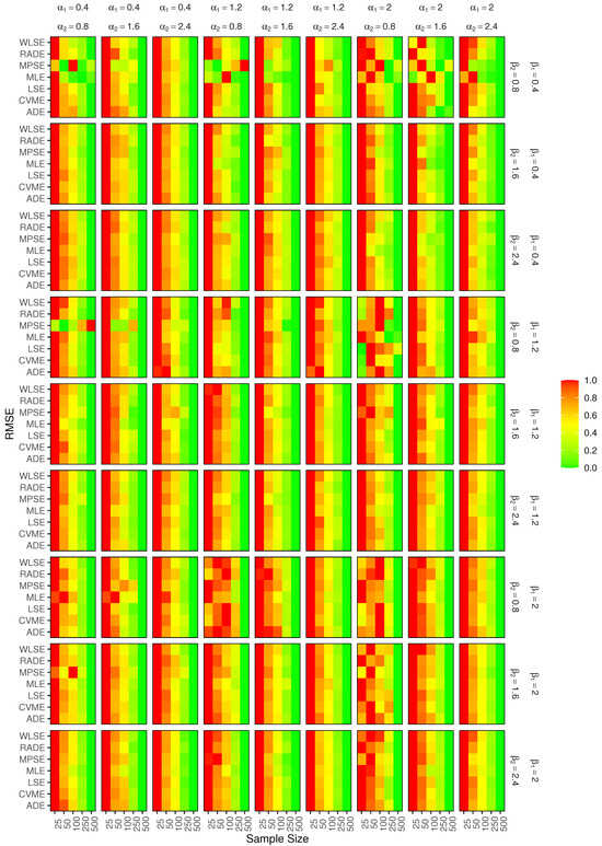
Figure 4. RMSE of the estimators of ${\alpha }_1$ for each estimation method and sample size. Color bars include numeric ticks; green indicates better performance (lower RMSE values), red indicates poorer accuracy (higher RMSE values).

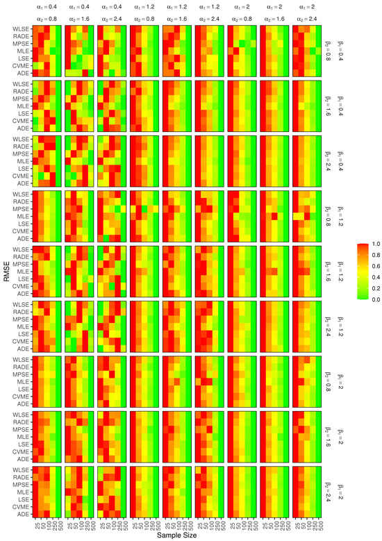
Figure 5. RMSE of the estimators of ${\alpha }_2$ for each estimation method and sample size. Color bars include numeric ticks; green indicates better performance (lower RMSE values), red indicates poorer accuracy (higher RMSE values).

Figure 6. RMSE of the estimators of ${\beta }_1$ for each estimation method and sample size. Color bars include numeric ticks; green indicates better performance (lower RMSE values), red indicates poorer accuracy (higher RMSE values).

Figure 7. RMSE of the estimators of ${\beta }_2$ for each estimation method and sample size. Color bars include numeric ticks; green indicates better performance (lower RMSE values), red indicates poorer accuracy (higher RMSE values).

• Generally, the RMSEs for the estimators of ${\beta }_2$ converges to 0 as the sample size increases starting from $n=100$. Nonetheless, in certain instances, we observe variations. For instance, when ${\alpha }_1=0.4, {\alpha }_2=2.4, {\beta }_1=1.2, {\beta }_2=0.8$, the RMSEs for the MPSEs initially (at $n=25$) exhibit small values, subsequently rise at moderate samples, and then decline once more.
• When ${\beta }_2$ exceeds 1, the RMSEs for the estimators of ${\beta }_1>1$ are minimal in large samples, indicating that the estimators are efficient, except when ${\alpha }_1=0.4, {\alpha }_2=2.4, {\beta }_1=1.2, {\beta }_2=2.4$, where the RMSEs for LSE, WLSE, and CVME are lower (close to 0) in small samples ($n=25, 50$) than in large samples ($n=250, 500$) where the values substantially increase to 1. In contrast, the RMSEs for ${\beta }_1<1$; in the first place, MPSEs exhibit reduced efficiency in certain situations, such as ${\alpha }_1=2, {\alpha }_2>1$, where at $n=250, 500$ the RMSEs are close to 1.
• When ${\beta }_2$ is less than 1, the RMSEs of the estimators of ${\beta }_1$ diminish as the sample gets larger, starting from color red $n=100$. Nevertheless, some methods yield more efficient estimators for small samples than the others. The RMSEs of the LSEs, WLSEs, CVMEs, ADEs, and RADEs are inferior to those of MLEs and MPSEs when ${\alpha }_1=0.4, {\alpha }_2=2.4, {\beta }_1=0.4, {\beta }_2=0.8$, where at $n=25, 50$, the RMSEs are extremely close to 0.
• Generally, the RMSEs of the estimators of ${\alpha }_1$, which decrease with a growth in sample size (starting from $n=100$, reflect the efficiency of the estimators’ performance. However, in some situations, some estimation approaches provide superior performance in small samples compared to other ones such as MPSEs in case of ${\alpha }_1=0.4, {\alpha }_2=0.8, {\beta }_1=0.4, {\beta }_2=0.8$, and MLEs when ${\alpha }_1=1.2, {\alpha }_2=0.8, {\beta }_1=0.4, {\beta }_2=0.8$, where RMSEs converge to 1 as sample size increases.
• When ${\alpha }_1$ is more than 1, the estimators of ${\alpha }_2$ show better performance with increasing sample size, regardless of the methods employed, but in most situations where ${\alpha }_1$ is less than 1, we observe variations in the RMSE values of ${\alpha }_2$ estimators, which are initially low at $n=25, 50$, which subsequently get higher at $n=100, 250$, and then decrease again at $n=500$.
• The presence of fluctuations in RMSEs across sample sizes might be attributed to several causes, such as sampling variability, the complexity of the lifetime distribution, and the sensitivity of the estimation methods to the underlying distribution characteristics, sample size, and sample variability. Smaller samples, by coincidence, may sometimes produce estimators with unexpectedly low RMSE; for instance, the sample might resemble the population well enough. As the sample size increases, the estimation procedure might be more susceptible to the specific sample realization and fail to reflect the underlying distribution’s characteristics.

The medians of RMSEs (denoted by $\mathrm{MRMSE}(·)$) were used as robust summary measures to compare the overall performance of the estimation methods across parameters and sample sizes. As shown in Table 6, the $\mathrm{MRMSE}$ values consistently decrease as the sample size increases, indicating improved estimation accuracy with larger samples. Among all methods, LS, CVM, AD, RAD, and WLS exhibit relatively low $\mathrm{MRMSE}$ values across parameters, reflecting stable and reliable performance. In contrast, MPS and particularly ML estimators yield considerably higher $\mathrm{MRMSE}$ values, especially for small and moderate sample sizes, suggesting slower or less stable convergence.

Table 6. Overall median of RMSEs per method across all sample sizes.

Method	n	$\mathbf{MRMSE}\left({\mathit{\alpha }}_1\right)$	$\mathbf{MRMSE}\left({\mathit{\alpha }}_2\right)$	$\mathbf{MRMSE}\left({\mathit{\beta }}_1\right)$	$\mathbf{MRMSE}\left({\mathit{\beta }}_2\right)$
AD	25	2.08	2.31	2.31	2.70
	50	1.85	2.02	1.48	1.83
	100	1.63	1.84	1.05	1.12
	250	1.23	1.53	0.73	0.68
	500	0.93	1.20	0.60	0.52
CVM	25	2.02	1.98	1.94	2.34
	50	1.55	1.62	1.20	1.46
	100	1.27	1.38	0.86	0.95
	250	1.03	1.14	0.60	0.63
	500	0.84	0.90	0.49	0.49
LS	25	1.84	1.95	1.60	1.81
	50	1.56	1.62	1.15	1.07
	100	1.30	1.38	0.80	0.86
	250	1.04	1.15	0.59	0.60
	500	0.85	0.92	0.52	0.48
ML	25	5.66	8.13	18.42	24.36
	50	3.72	6.20	10.43	17.86
	100	2.97	5.18	6.96	12.42
	250	2.50	3.71	4.24	7.53
	500	1.80	2.73	2.21	4.09
MPS	25	3.37	4.02	5.95	7.63
	50	2.67	3.70	4.38	5.18
	100	2.29	3.24	3.06	3.57
	250	1.78	2.38	2.13	2.53
	500	1.43	1.97	1.55	1.69
RAD	25	2.20	2.23	2.42	3.72
	50	1.68	1.97	1.64	2.56
	100	1.43	1.82	1.03	1.45
	250	1.02	1.56	0.66	0.84
	500	0.80	1.19	0.55	0.57
WLS	25	2.21	2.37	1.96	2.85
	50	1.91	2.11	1.43	2.01
	100	1.68	1.93	0.99	1.37
	250	1.28	1.58	0.77	0.88
	500	1.00	1.26	0.60	0.62

Overall, estimation precision improves with sample size, leading to smaller RMSEs. However, the observed fluctuations across estimators and parameters underscore the importance of selecting estimation methods that are suited to both the parameter regime and the available sample size.

4.2. Goodness-of-Fit Analysis

This section of the simulation results presents simulation results based on two simulated goodness-of-fit metrics: the average absolute difference ($D_{\mathrm{abs}}$) between the true and estimated cumulative distribution functions (CDFs), and the maximum absolute difference ($D_{\max }$) between the true and estimated CDFs, to evaluate the estimation methodologies. These metrics are defined as

$$D_{\mathrm{abs}}={\displaystyle \frac{1}{n\times N}}\sum _{i=1}^N\sum _{j=1}^n\left|F(x_j;\theta )-F(x_j;{\widehat{\theta }}_i)\right|$$

and

$$D_{\max }={\displaystyle \frac{1}{N}}\sum _{i=1}^N\underset{j=1,\dots ,n}{max}\left|F(x_j;\theta )-F(x_j;{\widehat{\theta }}_i)\right|$$

where ${\widehat{\theta }}_i$ denotes the estimate of the model parameter $\theta$ based on the i-th simulation run. The statistical measures $D_{\mathrm{abs}}$ and $D_{\max }$ are used to assess the accuracy of the estimation methods by quantifying the average and maximum absolute differences across all data points and simulation runs. Table 3, Table 4 and Table 5 include the estimated values of $D_{\max }$ and $D_{\mathrm{abs}}$ for three cases of parameters selected from simulation results. The simulated goodness-of-fit results are presented in Figure 8 and Figure 9. Both $D_{\mathrm{abs}}$ and $D_{\max }$ exhibit a decreasing trend as the sample size increases, regardless of the values of the shape parameters. Moreover, the values of $D_{\mathrm{abs}}$ and $D_{\max }$ are consistent across all estimators, indicating independence from the specific values of the shape parameter. While the RMSE values may not exhibit a perfectly monotonic convergence pattern, the comparison criteria based on $D_{\mathrm{abs}}$ and $D_{\max }$ indicate that all estimators achieve comparable distributional accuracy. The observed variation in parameter estimates arises because each method optimizes a different objective function. Despite these numerical differences, the resulting fitted distributions exhibit similar overall shapes and goodness-of-fit measures, confirming that the generalized gamma model adequately represents the data. Consequently, for larger sample sizes, all seven estimation procedures demonstrate reliable performance in capturing the underlying lifetime distribution.

Figure 8. Simulated $D_{\mathrm{abs}}$ for each estimation method and sample size. Color bars include numeric ticks; green indicates a better fit (lower $D_{\mathrm{abs}}$ values), red indicates a poorer fit (higher $D_{\mathrm{abs}}$ values).

Figure 9. Simulated $D_{\max }$ for each estimation method and sample size. Color bars include numeric ticks; green indicates a better fit (lower $D_{\max }$ values), red indicates a poorer fit (higher $D_{\max }$ values).

5. Data Analysis

This section illustrates the AGG distribution using real data in the health field. These real data are used to investigate the suggested estimation approaches and the practical applicability of the model. In addition to the RMSE, goodness-of-fit criteria such as Kolmogorov–Smirnov (KS) statistic and the corresponding p-value are used when analyzing the data. The preferred distribution is selected based on the lowest calculated criterion alongside the highest p-value. Because of estimating the parameters and existing ties in data, the corresponding p-value is calculated based on 1000 parametric bootstrap samples (see Algorithm 1).

Algorithm 1 Calculation of p-value

Require:  Observed data $\mathbf{X}=(x_1,\dots ,x_n)$, hypothesized CDF $F(x;\mathit{\theta })$, number of bootstrap replicates $B=1000$. Ensure:  Bootstrap-based p-values and Monte Carlo Standard Errors for the KS test. 1: Step 1: Estimate model parameters Obtain initial estimates $${\widehat{\theta }}^{\left(0\right)}=({\widehat{\alpha }}_1^{\left(0\right)},{\widehat{\alpha }}_2^{\left(0\right)},{\widehat{\beta }}_1^{\left(0\right)},{\widehat{\beta }}_2^{\left(0\right)},{\widehat{\lambda }}_1^{\left(0\right)},{\widehat{\lambda }}_2^{\left(0\right)})=({\widehat{\theta }}_1^{\left(0\right)},{\widehat{\theta }}_2^{\left(0\right)},{\widehat{\theta }}_3^{\left(0\right)},{\widehat{\theta }}_4^{\left(0\right)},{\widehat{\theta }}_5^{\left(0\right)},{\widehat{\theta }}_6^{\left(0\right)}),$$ for the seven estimation methods. 2: Step 2: Compute observed test statistic Using $F(x;\widehat{\mathit{\theta }})$, compute $T_{\mathrm{KS}}^{\left(0\right)}$. 3: Step 3: Parametric bootstrap simulation 4: for $b=1$ to B do 5:       Generate bootstrap sample $X^{\ast \left(b\right)}$ using the estimated parameters in step 1 6:       Re-estimate $${\widehat{\mathit{\theta }}}_j^{\ast \left(b\right)}=({\widehat{\alpha }}_{1j}^{\ast \left(b\right)},{\widehat{\alpha }}_{2j}^{\ast \left(b\right)},{\widehat{\beta }}_{1j}^{\ast \left(b\right)},{\widehat{\beta }}_{2j}^{\ast \left(b\right)},{\widehat{\lambda }}_{1j}^{\ast \left(b\right)},{\widehat{\lambda }}_{2j}^{\ast \left(b\right)})=({\widehat{\theta }}_{1j}^{\ast \left(b\right)},{\widehat{\theta }}_{2j}^{\ast \left(b\right)},{\widehat{\theta }}_{3j}^{\ast \left(b\right)},{\widehat{\theta }}_{4j}^{\ast \left(b\right)},{\widehat{\theta }}_{5j}^{\ast \left(b\right)},{\widehat{\theta }}_{6j}^{\ast \left(b\right)}),$$ based on bootstrap sample #j. 7:       Compute the KS test statistics $T_j^{\ast \left(b\right)}$ based on bootstrap sample #j. 8: end for 9: Step 4: Calculate bias of each estimator ${\widehat{\mathit{\theta }}}_i$ $${\mathrm{Bias}}^{\ast }\left({\widehat{\theta }}_i\right)={\displaystyle \frac{1}{B}}\sum _{j=1}^B{\widehat{\theta }}_{ij}^{\ast \left(b\right)}-\widehat{\theta }$$ 10: Step 5: Calculate RMSE for the estimator ${\widehat{\mathit{\theta }}}_i$ $${\mathrm{RMSE}}^{\ast }\left({\widehat{\theta }}_i\right)=\sqrt{{\displaystyle \frac{1}{B}}\sum _{i=1}^B{({\widehat{\theta }}_{ij}^{\ast \left(b\right)}-{\widehat{\theta }}_i)}^2}$$ 11: Step 6: Compute bootstrap p-values (mid-p correction) $$\widehat{p}={\displaystyle \frac{{\sum }_{b=1}^{B}I(T^{\ast \left(b\right)}>T^{\left(0\right)})+0.5{\sum }_{b=1}^{B}I(T^{\ast \left(b\right)}=T^{\left(0\right)})}{B}}$$ 12: Step 7: Compute Monte Carlo Standard Error (MCSE) $$\mathrm{MCSE}=\sqrt{{\displaystyle \frac{\widehat{p}(1-\widehat{p})}{B}}}$$

The first dataset in Table 7 consists of the survival times in days of 43 patients with blood cancer obtained from the Ministry of Health Hospital in Saudi Arabia, studied by [75]. The data are transformed from days to years for computational convenience. The second dataset in Table 8 consists of survival times of 30 patients with chronic granulocytic (CG) leukemia, as cited in the National Cancer Institute [76]. Both datasets represent complete samples of uncensored survival times. No additional information was available in the original sources regarding disease subtypes, treatment protocols, or specific causes of death. Consequently, these datasets are interpreted as pure lifetime data, where the observed failures are assumed to result from either disease progression (Cause #1) or other complications (Cause #2), both of which are unknown. The summary statistics of the two datasets are obtained in Table 9. The histogram and box-plot for each dataset are shown in Figure 10.

Table 7. Survival times in days of blood cancer data.

115	181	225	418	441	461	516	739	743	789	807	865	924
983	1025	1062	1063	1063	1165	1191	1222	1222	1251	1277	1290	1357
1369	1408	1455	1478	1519	1578	1578	1599	1603	1605	1696	1735	1799
1815	1852	1899	1925	1965

Table 8. Survival times of chronic granulocytic leukemia.

0.019	0.129	0.159	0.203	0.485	0.635	0.747	1.054	0.868	1.175
1.205	1.218	1.246	1.117	1.355	1.361	1.457	1.563	1.585	1.591
1.780	1.922	1.958	2.133	2.412	2.464	2.546	2.650	2.949	3.036

Table 9. Summary statistics for blood cancer and CG leukemia datasets.

Data	n	Min	Max	Mean	Median	SD	Q1	Q3	Skew	Kurt
Blood Cancer	43	0.315	5.384	3.265	3.427	1.388	2.290	4.352	−0.427	−0.826
CG Leukemia	30	0.019	3.036	1.434	1.358	0.839	0.915	1.949	0.138	−0.886

Figure 10. The histogram and box-plot of blood cancer and CG luekemia.

For blood cancer data, the estimated model parameters employing the seven estimation methods are listed in Table 10. The variation in RMSEs is observed across parameters within the same method, with no specific approach providing uniformly optimal estimates for all parameters. ML procedure exhibited the highest RMSE for ${\alpha }_1$, while performing well for ${\alpha }_2$, ${\lambda }_1$, and ${\lambda }_2$. MPS approach showed the greatest RMSEs for ${\beta }_1$, ${\beta }_2$, and ${\lambda }_2$. AD and RAD methods delivered close estimates as well as close RMSEs for all parameters except ${\alpha }_1$ where their RMSEs are not the least.

Table 10. The estimated values of the parameters with their RMSEs based on blood cancer data.

Method	${\widehat{\mathit{\alpha }}}_1$	RMSE (${\widehat{\mathit{\alpha }}}_1$)	${\widehat{\mathit{\alpha }}}_2$	RMSE (${\widehat{\mathit{\alpha }}}_2$)	${\widehat{\mathit{\beta }}}_1$	RMSE (${\widehat{\mathit{\beta }}}_1$)
ML	15.4198	4.7328	0.1346	0.0176	19.5595	1.1825
LS	1.9709	0.6654	0.2843	0.1011	3.3681	1.2106
WLS	0.5241	0.3320	0.4246	0.1583	7.5364	3.1230
MPS	0.2104	0.2998	0.1664	0.0841	14.6875	7.8276
CVM	0.9462	0.2262	0.3919	0.1191	5.5023	1.9429
AD	4.7561	1.4691	0.3897	0.0226	3.4650	0.2226
RAD	4.7561	1.2981	0.3897	0.0313	3.4650	0.2229
Method	${\widehat{\mathit{\beta }}}_{\mathbf{2}}$	RMSE (${\widehat{\mathit{\beta }}}_{\mathbf{2}}$)	${\widehat{\mathit{\lambda }}}_{\mathbf{1}}$	RMSE (${\widehat{\mathit{\lambda }}}_{\mathbf{1}}$)	${\widehat{\mathit{\lambda }}}_{\mathbf{2}}$	RMSE (${\widehat{\mathit{\lambda }}}_{\mathbf{2}}$)
ML	12.0944	0.8190	4.6413	0.0095	5.3892	0.0036
LS	3.9677	0.8151	3.7254	0.5858	8.9501	7.2845
WLS	2.5018	0.8302	5.0442	0.5480	10.8580	9.2035
MPS	6.2028	2.5793	5.4121	0.4417	11.2521	15.7041
CVM	3.1899	0.7191	4.6866	0.3683	8.1690	4.8736
AD	4.2266	0.5491	3.1727	0.0819	5.6192	0.0004
RAD	4.2267	0.7237	3.1727	0.0030	5.6192	0.0005

The goodness-of-fit metrics based on the observed blood cancer data are studied and the results are listed in Table 11. The quantile–quantile (Q-Q) plot between the estimated and empirical distribution functions is provided in Figure 11. Obviously, all the estimation methods yielded close test statistics KS, demonstrating a good distributional fit. The p-values for AD, RAD, and ML methods are the highest compared to others. The MCSE refers to how uncertain $\widehat{p}$ is because of using a finite number of simulations B. It is the standard error of “successes” that represents the number of bootstrap statistics greater than or equal to the observed statistic. The MCSEs corresponding to AD, RAD, and ML are the least, indicating their p-values are the most confident.

Table 11. Outcomes of goodness-of-fit statistics based on blood cancer data.

Method	KS	Sig.	MCSE
ML	0.0590	0.9980	0.0014
LS	0.0533	0.7720	0.0133
WLS	0.0562	0.7070	0.0144
MPS	0.0680	0.5486	0.0157
CVM	0.0482	0.8360	0.0117
AD	0.0546	0.9980	0.0014
RAD	0.0546	0.9980	0.0014

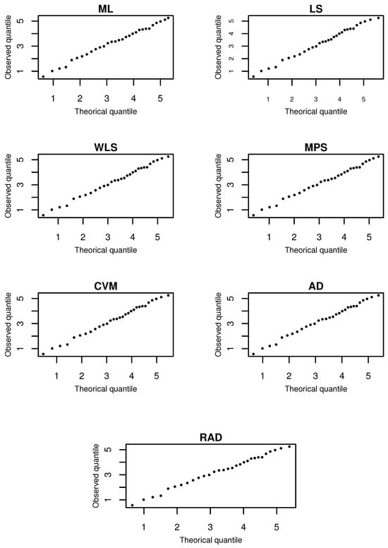
Figure 11. The Q-Q plot of fitted models based on blood cancer data.

Based on CG leukemia data, the calculated values of the model’s parameters using the previously described approaches are listed in Table 12. The variation in estimates, as well as within the corresponding RMSEs, is obvious. The MPS method produced estimates with the highest RMSEs corresponding to ${\alpha }_1$ and ${\beta }_1$, while RMSEs of MLEs of ${\alpha }_2$ and ${\beta }_2$ are the least efficient. Although there was no systemic pattern among the performance of estimates that concluded a specific approach that could provide uniformly optimal estimates for all parameters, generally, AD provided more accurate estimates according to their RMSEs, despite the RMSE of ${\beta }_2$ and ${\lambda }_2$, which provided a slight rise higher than those of RAD.

Table 12. The estimated values of the parameters with their RMSEs based on CG leukemia.

Method	${\widehat{\mathit{\alpha }}}_1$	RMSE (${\widehat{\mathit{\alpha }}}_1$)	${\widehat{\mathit{\alpha }}}_2$	RMSE (${\widehat{\mathit{\alpha }}}_2$)	${\widehat{\mathit{\beta }}}_1$	RMSE (${\widehat{\mathit{\beta }}}_1$)
ML	3.6116	2.0087	4.5149	4.3490	1.4248	2.4111
LS	5.6439	2.2234	2.4974	1.5427	0.8975	1.8302
WLS	5.5375	2.4516	2.3260	1.4963	0.9521	2.0398
MPS	7.9532	3.8635	2.6522	1.4514	0.8686	3.8197
CVM	5.8527	2.1115	2.4623	1.6501	0.9190	1.9793
AD	5.8995	1.8341	2.8161	0.6759	0.9653	1.4100
RAD	2.1265	3.2239	2.5949	1.2476	1.5031	2.7793
Method	${\widehat{\mathit{\beta }}}_{\mathbf{2}}$	RMSE (${\widehat{\mathit{\beta }}}_{\mathbf{2}}$)	${\widehat{\mathit{\lambda }}}_{\mathbf{1}}$	RMSE (${\widehat{\mathit{\lambda }}}_{\mathbf{1}}$)	${\widehat{\mathit{\lambda }}}_{\mathbf{2}}$	RMSE (${\widehat{\mathit{\lambda }}}_{\mathbf{2}}$)
ML	0.2247	6.7958	0.7578	2.3817	0.0097	1.3849
LS	0.1711	1.2295	0.2500	1.1269	0.7326	1.6041
WLS	0.2324	0.9868	0.2931	1.1452	0.9150	1.6447
MPS	0.2429	1.3092	0.1666	1.2357	0.2893	2.9476
CVM	0.2121	1.6168	0.2494	1.1298	0.8880	1.4492
AD	0.2553	1.0894	0.2825	0.7728	0.2715	1.0647
RAD	0.1755	0.8938	1.0638	0.9062	0.8675	0.7490

The results of goodness-of-fit tests are shown in Table 13, while the Q-Q plot is shown in Figure 12. All methods produced adequate distributional fits according to test statistics, but AD showed outstanding performance based on the corresponding p-value and MCSE.

Table 13. Outcomes of goodness-of-fit statistics based on CG leukemia data.

Method	KS	Sig.	MCSE
ML	0.0897	0.5350	0.0158
LS	0.0776	0.6490	0.0151
WLS	0.0804	0.5660	0.0157
MPS	0.0895	0.6780	0.0148
CVM	0.0729	0.6820	0.0147
AD	0.0777	0.7990	0.0127
RAD	0.0776	0.6260	0.0153

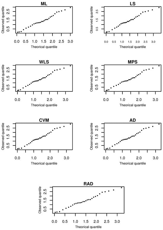
Figure 12. The Q-Q plot of fitted models based on CG leukemia data.

The evaluations revealed that some approaches provided better parameter estimation accuracy (lower RMSE). At the same time, other methods showed superior distributional approximation (better goodness-of-fit results) as demonstrated in the first application, where ML exhibited goodness-of-fit results and the highest RMSE of $\alpha$. The conflict between the estimation efficiency of the parameters and the performance of the goodness-of-fit test is not a problem to be solved; it is expected, especially when dealing with complex distributions. The results demonstrated the ability of unstable parameters to produce better distributional fits and provide adaptation to limited data. Based on analysis of two datasets, AD achieved a best fit with more accurate estimates. The choice of optimal methods depends on the purpose of the analysis, whether it is parameter inference or distributional modeling. For clinical data analysis, goodness-of-fit tests are the primary recommendation since decisions depend on distributional accuracy, risk evaluation requires accurate distributional behavior, and predictive performance is more critical than parameter precision.

6. Conclusions

In this paper, a competing risks model based on Stacy’s GG distribution is proposed, considering two latent failure times with different shapes and scale parameters. The model parameters are estimated using seven methods, and a free derivative procedure is utilized to optimize the objective functions of these methods. The accuracy of estimates is evaluated through the examination of their RMSEs. The results showed fluctuations in the values of the RMSEs for all estimation approaches, indicating a non-systematic pattern across different sample sizes. The existence and uniqueness of the estimators remain analytically intractable and represent an open problem. The model complexity and potential parameter interactions may lead to flat or multimodal likelihood surfaces. Further research could explore parameter identifiability through profile likelihoods or Fisher information analysis. To assess distributional fit quality, the KS test is considered, and the results revealed that while individual parameter estimates exhibited variations across samples, the overall distributional form remains consistent.

One of the most significant challenges faced by physicians in clinical research is accurately diagnosing diseases to design effective treatment plans, while also considering the factors that interfere with patients’ lives. For the application part, two real datasets from the clinical field are used to study the applicability of the proposed competing risks model (AGG distribution). The different estimation methods yielded substantially different parameter estimates, even with the same initial values as well as RMSEs. The methods, in general, produced adequate distributional fits despite the inaccuracy of their estimates; however, based on data analysis, AD showed superior performance and an excellent fit. It is preferable to consider the method that provides a better distributional approximation, allowing for accurate capture of data patterns and reliable clinical predictions.

References

- Loscalzo, J.; Fauci, A.S.; Kasper, D.L.; Hauser, S.; Longo, D.L. Harrison’s Principles of Internal Medicine, 21st ed.; McGraw-Hill Education: New York, NY, USA, 2022; Volumes 1 and 2. [Google Scholar]
- International Agency for Research on Cancer. Global Cancer Observatory: Cancer Today. 2018. Available online: https://gco.iarc.fr/today (accessed on 3 October 2025).
- Cox, D.R. The Analysis of Exponentially Distributed Life-Times with Two Types of Failure. J. R. Stat. Soc. Ser. B (Methodol.) 1959, 21, 411–421. [Google Scholar] [CrossRef]
- Crowder, M.J. Classical Competing Risks; Chapman and Hall/CRC: Boca Raton, FL, USA, 2001. [Google Scholar] [CrossRef]
- Almarashi, A.M.; Algarni, A.; Daghistani, A.M.; Abd-Elmougod, G.A.; Abdel-Khalek, S.; Raqab, M.Z. Inferences for Joint Hybrid Progressive Censored Exponential Lifetimes under Competing Risk Model. Math. Probl. Eng. 2021, 2021, 3380467. [Google Scholar] [CrossRef]
- Davies, K.F.; Volterman, W. Progressively Type-II censored competing risks data from the linear exponential distribution. Commun. Stat.—Theory Methods 2020, 51, 1444–1460. [Google Scholar] [CrossRef]
- Nassar, M.; Alotaibi, R.; Dey, S. Estimation Based on Adaptive Progressively Censored under Competing Risks Model with Engineering Applications. Math. Probl. Eng. 2022, 2022, 6731230. [Google Scholar] [CrossRef]
- Alghamdi, A.S.; Abd-Elmougod, G.A.; Kundu, D.; Marin, M. Statistical Inference of Jointly Type-II Lifetime Samples under Weibull Competing Risks Models. Symmetry 2022, 14, 701. [Google Scholar] [CrossRef]
- Ramadan, D.A.; Almetwally, E.M.; Tolba, A.H. Statistical Inference to the Parameter of the Akshaya Distribution under Competing Risks Data with Application HIV Infection to AIDS. Ann. Data Sci. 2022, 10, 1499–1525. [Google Scholar] [CrossRef]
- Farghal, A.W.A.; Badr, S.K.; Abu-Zinadah, H.; Abd-Elmougod, G.A. Analysis of generalized inverted exponential competing risks model in presence of partially observed failure modes. Alex. Eng. J. 2023, 78, 74–87. [Google Scholar] [CrossRef]
- Elshahhat, A.; Nassar, M. Inference of improved adaptive progressively censored competing risks data for Weibull lifetime models. Stat. Pap. 2023, 65, 1163–1196. [Google Scholar] [CrossRef]
- Dutta, S.; Ng, H.K.T.; Kayal, S. Inference for Kumaraswamy-G family of distributions under unified progressive hybrid censoring with partially observed competing risks data. Stat. Neerl. 2024, 78, 719–742. [Google Scholar] [CrossRef]
- Park, C.; Wang, M. Parameter Estimation of Birnbaum-Saunders Distribution under Competing Risks Using the Quantile Variant of the Expectation-Maximization Algorithm. Mathematics 2024, 12, 1757. [Google Scholar] [CrossRef]
- Alotaibi, R.; Rezk, H.; Park, C. Parameter estimation of inverse Weibull distribution under competing risks based on the expectation–maximization algorithm. Qual. Reliab. Eng. Int. 2024, 40, 3795–3808. [Google Scholar] [CrossRef]
- Alhidairah, S.; Alam, F.M.A.; Nassar, M. A new competing risks model with applications to blood cancer data. J. Radiat. Res. Appl. Sci. 2024, 17, 101001. [Google Scholar] [CrossRef]
- Ahmed, S.M.; Abdalla, M.; Farghal, A.W.A. Statistical inference for competing risks model with Type-II generalized hybrid censored of inverse Lomax distribution with applications. Alex. Eng. J. 2025, 118, 132–146. [Google Scholar] [CrossRef]
- Alotaibi, R.; Nassar, M.; Khan, Z.A.; Alajlan, W.A.; Elshahhat, A. Analysis and data modelling of electrical appliances and radiation dose from an adaptive progressive censored XGamma competing risk model. J. Radiat. Res. Appl. Sci. 2025, 18, 101188. [Google Scholar] [CrossRef]
- Ranjan, R.; Singh, S.; Upadhyay, S.K. A Bayes analysis of a competing risk model based on gamma and exponential failures. Reliab. Eng. Syst. Saf. 2015, 144, 35–44. [Google Scholar] [CrossRef]
- Ranjan, R.; Upadhyay, S.K. Classical and Bayesian Estimation for the Parameters of a Competing Risk Model Based on Minimum of Exponential and Gamma Failures. IEEE Trans. Reliab. 2016, 65, 1522–1535. [Google Scholar] [CrossRef]
- Jayakodi, G.; Sundaram, N.; Venkatesan, P. Parametric Regression Modeling of Competing Risk Using Cardiovascular Disease Patient’s Survival Data. JP J. Biostat. 2022, 22, 25–47. [Google Scholar] [CrossRef]
- Stacy, E.W. A Generalization of the Gamma Distribution. Ann. Math. Stat. 1962, 33, 1187–1192. [Google Scholar] [CrossRef]
- Balakrishnan, N.; Peng, Y. Generalized gamma frailty model. Stat. Med. 2006, 25, 2797–2816. [Google Scholar] [CrossRef]
- Barkauskas, D.A.; Kronewitter, S.R.; Lebrilla, C.B.; Rocke, D.M. Analysis of MALDI FT-ICR mass spectrometry data: A time series approach. Anal. Chim. Acta 2009, 648, 207–214. [Google Scholar] [CrossRef] [PubMed]
- Khakifirooz, M.; Tseng, S.T.; Fathi, M. Model Mis-Specification of Generalized Gamma Distribution for Accelerated Lifetime Censored Data. Technometrics 2020, 62, 357–370. [Google Scholar] [CrossRef]
- Chang, I.H.; Kim, B.H. Non-informative priors in the generalized gamma stress-strength systems. IIE Trans. 2011, 43, 797–804. [Google Scholar] [CrossRef]
- Ortega, E.M.M.; Bolfarine, H.; Paula, G.A. Influence diagnostics in generalized log-gamma regression models. Comput. Stat. Data Anal. 2003, 42, 165–186. [Google Scholar] [CrossRef]
- Jordanova, P.K.; Savov, M.; Tchorbadjieff, A.; Stehlík, M. Mixed Poisson process with Stacy mixing variable. arXiv 2024, arXiv:2303.10226v1. [Google Scholar] [CrossRef]
- Tahai, A.; Meyer, M.J. A Revealed Preference Study of Management Journals’ Direct Influences. Strateg. Manag. J. 1999, 20, 279–296. [Google Scholar] [CrossRef]
- van Noortwijk, J.M. Bayes Estimates of Flood Quantiles using the Generalised Gamma Distribution. In System and Bayesian Reliability; Essays in Honor of Professor Richard E. Barlow on His 70th Birthday; Hayakawa, Y., Irony, T., Xie, M., Eds.; World Scientific Publishing: Singapore, 2001; pp. 351–374. [Google Scholar]
- Shin, J.W.; Chang, J.H.; Yun, H.S.; Kim, N.S. Voice Activity Detection Based on Generalized Gamma Distribution. In Proceedings of the IEEE International Conference on Acoustics, Speech, and Signal Processing (ICASSP), Philadelphia, PA, USA, 23 March 2005; IEEE: New York, NY, USA, 2005; pp. I-781–I-784. [Google Scholar]
- Shanker, R.; Shukla, K.K. On Modeling Of Lifetime Data Using Three-Parameter Generalized Lindley and Generalized Gamma Distributions. Biom. Biostat. Int. J. 2016, 4, 283–288. [Google Scholar] [CrossRef]
- Pending, A.N. Modeling traumatic brain injury lifetime data: Improved estimators for the Generalized Gamma distribution under small samples. PLoS ONE 2019, 14, e0221332. [Google Scholar] [CrossRef]
- Zamani, H.; Shekari, M.; Pakdaman, Z. Modeling insurance data using generalized gamma regression. J. Stat. Model. Theory Appl. 2020, 1, 169–177. [Google Scholar]
- Ulusoy, I.C.; Erdik, T. Marine current energy estimation using the generalized gamma distribution: A case study for the upper layer of the Dardanelles Strait. J. Ocean. Eng. Mar. Energy 2021, 7, 481–492. [Google Scholar] [CrossRef]
- Peng, C. A New Formulation of Generalized Gamma: Some Results and Applications. ESAIM Probab. Stat. 2023, 27, 913–935. [Google Scholar] [CrossRef]
- Fidelis, C.R.; Ortega, E.M.M.; Prataviera, F.; Vila, R.; Cordeiro, G.M. Reparametrized generalized gamma partially linear regression with application to breast cancer data. J. Appl. Stat. 2024, 51, 3248–3265. [Google Scholar] [CrossRef]
- Ferreira, A.A.; Cordeiro, G.M. The Flexible Generalized Gamma Distribution with Applications to COVID-19 Data. Rev. Colomb. Estadística 2024, 47, 453–473. [Google Scholar] [CrossRef]
- Prentice, R.L. A log gamma model and its maximum likelihood estimation. Biometrika 1974, 61, 539–544. [Google Scholar] [CrossRef]
- Arslan, T.; Acitas, S.; Senoglu, B. On the maximization of the likelihood for the generalized gamma distribution: The modified maximum likelihood approach. Soft Comput. 2025, 29, 579–591. [Google Scholar] [CrossRef]
- Gupta, R.D.; Kundu, D. Generalized exponential distribution: Different method of estimations. J. Stat. Comput. Simul. 2001, 69, 315–337. [Google Scholar] [CrossRef]
- Alkasasbeh, M.R.; Raqab, M.Z. Estimation of the generalized logistic distribution parameters: Comparative study. Stat. Methodol. 2009, 6, 262–279. [Google Scholar] [CrossRef]
- Mazucheli, J.; Louzada, F.; Ghitany, M. Comparison of estimation methods for the parameters of the weighted Lindley distribution. Appl. Math. Comput. 2013, 220, 463–471. [Google Scholar] [CrossRef]
- do Espirito Santo, A.; Mazucheli, J. Comparison of estimation methods for the Marshall–Olkin extended Lindley distribution. J. Stat. Comput. Simul. 2014, 85, 3437–3450. [Google Scholar] [CrossRef]
- Balakrishnan, N.; Alam, F.M.A. Maximum likelihood estimation of the parameters of Student’s t Birnbaum-Saunders distribution: A comparative study. Commun. Stat. Simul. Comput. 2019, 51, 793–822. [Google Scholar] [CrossRef]
- Alam, F.M.A.; Nassar, M. On Modeling Concrete Compressive Strength Data Using Laplace Birnbaum-Saunders Distribution Assuming Contaminated Information. Crystals 2021, 11, 830. [Google Scholar] [CrossRef]
- Moloy, D.J.; Ali, M.A.; Alam, F.M.A. Modeling Climate data using the Quartic Transmuted Weibull Distribution and Different Estimation Methods. Pak. J. Stat. Oper. Res. 2023, 19, 649–669. [Google Scholar] [CrossRef]
- Alosaimi, B.S.; Alam, F.M.; Baaqeel, H.M. Modeling Air Pollution Data Using a Generalized Birnbaum-Saunders Distribution with Different Estimation Procedures. In Mathematical Modeling in Physical Sciences; Springer Nature: Cham, Switzerland, 2024; pp. 587–618. [Google Scholar] [CrossRef]
- Alam, F.M.A. On Modeling X-Ray Diffraction Intensity Using Heavy-Tailed Probability Distributions: A Comparative Study. Crystals 2025, 15, 188. [Google Scholar] [CrossRef]
- Klutke, G.; Kiessler, P.; Wortman, M. A critical look at the bathtub curve. IEEE Trans. Reliab. 2003, 52, 125–129. [Google Scholar] [CrossRef]
- Gurvich, M.R.; Dibenedetto, A.T.; Ranade, S.V. A new statistical distribution for characterizing the random strength of brittle materials. J. Mater. Sci. 1997, 32, 2559–2564. [Google Scholar] [CrossRef]
- Nadarajah, S.; Kotz, S. On Some Recent Modifications of Weibull Distribution. IEEE Trans. Reliab. 2005, 54, 561–562. [Google Scholar] [CrossRef]
- Lai, C.; Xie, M.; Murthy, D. Reply to “On Some Recent Modifications of Weibull Distribution”. IEEE Trans. Reliab. 2005, 54, 563. [Google Scholar] [CrossRef]
- Xie, M.; Lai, C. Reliability analysis using an additive Weibull model with bathtub-shaped failure rate function. Reliab. Eng. Syst. Saf. 1996, 52, 87–93. [Google Scholar] [CrossRef]
- Lemonte, A.J.; Cordeiro, G.M.; Ortega, E.M.M. On the Additive Weibull Distribution. Commun. Stat.—Theory Methods 2014, 43, 2066–2080. [Google Scholar] [CrossRef]
- Ahmad, A.E.B.A.; Ghazal, M. Exponentiated additive Weibull distribution. Reliab. Eng. Syst. Saf. 2020, 193, 106663. [Google Scholar] [CrossRef]
- Friedman, H. A consistent Fubini-Tonelli theorem for nonmeasurable functions. Ill. J. Math. 1980, 24. [Google Scholar] [CrossRef]
- Priestley, H.A. Fubini’s Theorem and Tonelli’s Theorem. In Introduction to Integration; Oxford University Press: Oxford, UK, 1997; pp. 190–200. [Google Scholar] [CrossRef]
- Olver, F.W.J.; Olde Daalhuis, A.B.; Lozier, D.W.; Schneider, B.I.; Boisvert, R.F.; Clark, C.W.; Miller, B.R.; Saunders, B.V.; Cohl, H.S.; McClain, M.A. (Eds.) NIST Digital Library of Mathematical Functions; Release 1.2.3 of 2024-12-15. Available online: https://dlmf.nist.gov/ (accessed on 19 November 2025).
- Kelley, C.T. Solving Nonlinear Equations with Newton’s Method; Society for Industrial and Applied Mathematics: Philadelphia, PA, USA, 2003. [Google Scholar] [CrossRef]
- Brent, R.P. An algorithm with guaranteed convergence for finding a zero of a function. Comput. J. 1971, 14, 422–425. [Google Scholar] [CrossRef]
- Chen, C.M.; Lin, C.C.; Wu, C.C.; Tsai, J.R. Mixture mean residual life model for competing risks data with mismeasured covariates. J. Appl. Stat. 2024, 52, 1361–1380. [Google Scholar] [CrossRef]
- Watson, G.S.; Wells, W.T. On the Possibility of Improving the Mean Useful Life of Items by Eliminating Those with Short Lives. Technometrics 1961, 3, 281–298. [Google Scholar] [CrossRef]
- Cheng, R.C.H.; Amin, N.A.K. Maximum Product-of-Spacings Estimation with Applications to the Lognormal Distribution; Technical Report 1; Department of Mathematics, University of Wales IST: Wales, UK, 1979. [Google Scholar]
- Cheng, R.C.H.; Amin, N.A.K. Estimating Parameters in Continuous Univariate Distributions with a Shifted Origin. J. R. Stat. Soc. Ser. B Stat. Methodol. 1983, 45, 394–403. [Google Scholar] [CrossRef]
- Ranneby, B. The Maximum Spacing Method. An Estimation Method Related to the Maximum Likelihood Method. Scand. J. Stat. 1984, 11, 93–112. [Google Scholar]
- Ghosh, K.; Jammalamadaka, S. A general estimation method using spacings. J. Stat. Plan. Inference 2001, 93, 71–82. [Google Scholar] [CrossRef]
- Murage, P.; Mung’atu, J.; Odero, E. Optimal Threshold Determination for the Maximum Product of Spacing Methodology with Ties for Extreme Events. Open J. Model. Simul. 2019, 07, 149–168. [Google Scholar] [CrossRef]
- Swain, J.; Venkatraman, S.; Wilson, J. Least squares estimation of distribution function in Johnson’s translation system. J. Stat. Comput. Simul. 1988, 29, 271–297. [Google Scholar] [CrossRef]
- Arnold, B.C.; Balakrishnan, N.; Nagaraja, H.N. A First Course in Order Statistics; SIAM: Philadelphia, PA, USA, 2008. [Google Scholar]
- Boos, D.D. Minimum Distance Estimation in Nonlinear Regression. Ann. Stat. 1982, 10, 826–837. [Google Scholar]
- Posit team. RStudio: Integrated Development Environment for R; Posit Software, PBC: Boston, MA, USA, 2025. [Google Scholar]
- R Core Team. R: A Language and Environment for Statistical Computing; R Foundation for Statistical Computing: Vienna, Austria, 2025. [Google Scholar]
- Johnson, S.G. The NLopt Nonlinear-Optimization Package. 2007. Available online: https://github.com/stevengj/nlopt (accessed on 22 July 2025).
- Powell, M. The BOBYQA Algorithm for Bound Constrained Optimization without Derivatives; Technical Report; Department of Applied Mathematics and Theoretical Physics, University of Cambridge: Cambridge, UK, 2009. [Google Scholar]
- Abouammoh, A.; Abdulghani, S.; Qamber, I. On partial orderings and testing of new better than renewal used classes. Reliab. Eng. Syst. Saf. 1994, 43, 37–41. [Google Scholar] [CrossRef]
- Bryson, M.C.; Siddiqui, M. Some Criteria for Aging. J. Am. Stat. Assoc. 1969, 64, 147–161. [Google Scholar] [CrossRef]
Disclaimer/Publisher’s Note: The statements, opinions and data contained in all publications are solely those of the individual author(s) and contributor(s) and not of MDPI and/or the editor(s). MDPI and/or the editor(s) disclaim responsibility for any injury to people or property resulting from any ideas, methods, instructions or products referred to in the content. |
© 2025 by the authors. Licensee MDPI, Basel, Switzerland. This article is an open access article distributed under the terms and conditions of the Creative Commons Attribution (CC BY) license (https://creativecommons.org/licenses/by/4.0/).