Multi-Objective Mathematical Model for Crude Oil Terminal Scheduling with Tank Farm Operations

Abstract

A critical process underpinning the sustainability of the global economy is the reliable and efficient supply of crude oil from tank farms to international markets. The crude oil terminal serves as the central component of this process. The availability of crude oil in tank farms and the scheduling of oil carriers are key operational decisions made at the oil terminals. This study introduces a novel multi-objective mixed-integer programming (MIP) model for Crude Oil Terminal Scheduling (COTS). The model is an extension of our earlier mathematical modeling framework on COTS. The primary objective of the proposed COTS model is to enhance customer satisfaction by reducing the deviation between actual loading dates and customers’ preferred loading dates. Secondary objectives include managing crude oil inventory levels and reducing the frequency of tank service changes. The model’s results support decision-makers in both scheduling oil carriers and allocating tank storage capacities while enabling dynamic adjustments of tank operations across multiple crude oil types. To address multiple objectives, in this work, several solution approaches, namely the weighted sum (WS) approach, the hierarchical optimization (HO) approach, and the weighted Tchebycheff (WT) approach, are developed. Novel ordering and scaling methods in handling the multiple objectives for COTS using HO and WT are proposed in this paper. The validity of the proposed model and the effectiveness of its solutions are demonstrated through a numerical case study. Based on the numerical analysis, it is estimated that the Pareto-based approaches like HO and WT increase the solution time by ≈400% in the presence of four objectives. However, the Pareto approaches provide a spectrum of operational points to the decision-maker. Finally, key findings and future research paths are discussed.

1. Introduction

They say money moves the world, but energy makes it function, and oil plays a significant role in global energy consumption. Oil contributes to various sectors, including transportation, industry, and electricity generation. The consumption of oil is strongly correlated with improved quality of life, as measured by the United Nations Human Development Index (HDI). 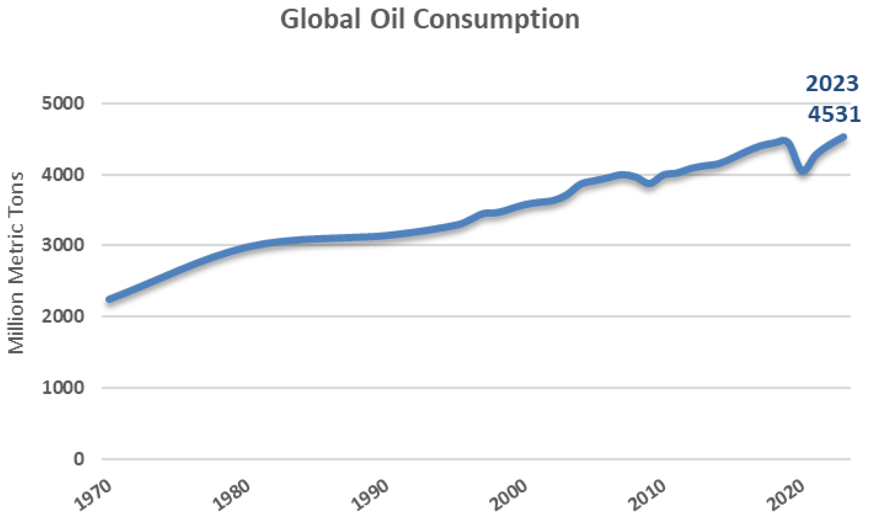Countries with higher oil consumption tend to have populations that are better educated, wealthier, and longer-lived [1]. Moreover, since the 1970s, oil consumption across the world has been gradually increasing over the years [2], as shown in Figure 1.

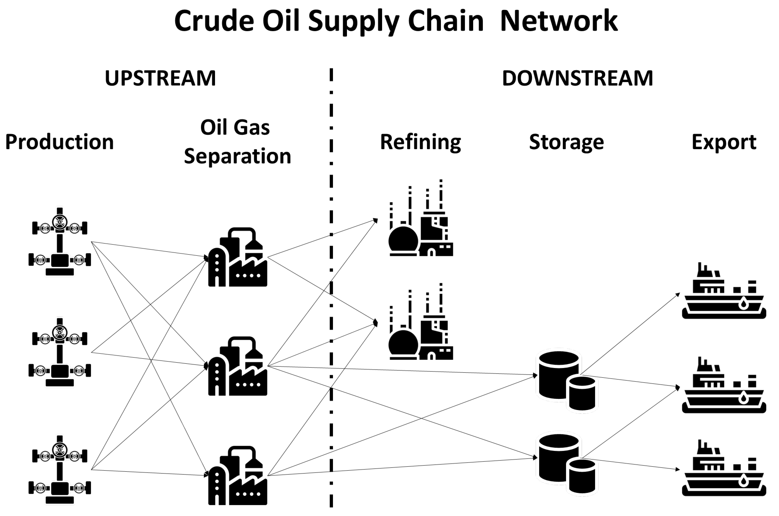
The crude oil industry involves the process from the point of detection of crude oil to the final delivery to customers across the world. The crude oil industry is usually divided into two segments, upstream and downstream. Each segment includes a large network of equipment and facilities for crude oil production, treatment, processing, and transportation. In the upstream segment, the crude oil is produced from oil fields and sent to be treated in oil and gas separation plants, where the gas and water associated with the crude oil are removed. The downstream segment starts with treated crude oil that supplies different facilities through pipelines. Those facilities can be refineries where the crude oil is processed or crude oil terminals (COT) where it is stored and shipped to customers using crude oil carriers, as illustrated in Figure 2 [3,4].

Terminals, in the crude oil industry, guarantee a sustainable and efficient supply of crude oil from the tank farms to the rest of the world and play a decisive role in sustaining the global economy. They are essential infrastructure that facilitates the storage, distribution, and transportation of crude oil globally. These terminals serve as critical hubs, connecting production sites to refineries and consumers to ensure reliable and efficient movement of this vital energy resource, supporting economic growth and development worldwide. The strategic planning and operational efficiency of crude oil terminals are crucial in maintaining a stable and secure energy supply, which is fundamental to the functioning of modern societies. The research question in the crude oil industry can be stated as follows: can a data-driven automated scheduling model improve operational efficiency and reduce delays in crude oil terminals compared to traditional manual scheduling methods? Currently, there is no data-driven and automated approach directly applicable to scheduling operations in crude oil terminals reported in the literature. This work aims to bridge that gap by proposing a model designed to support day-to-day terminal operations.

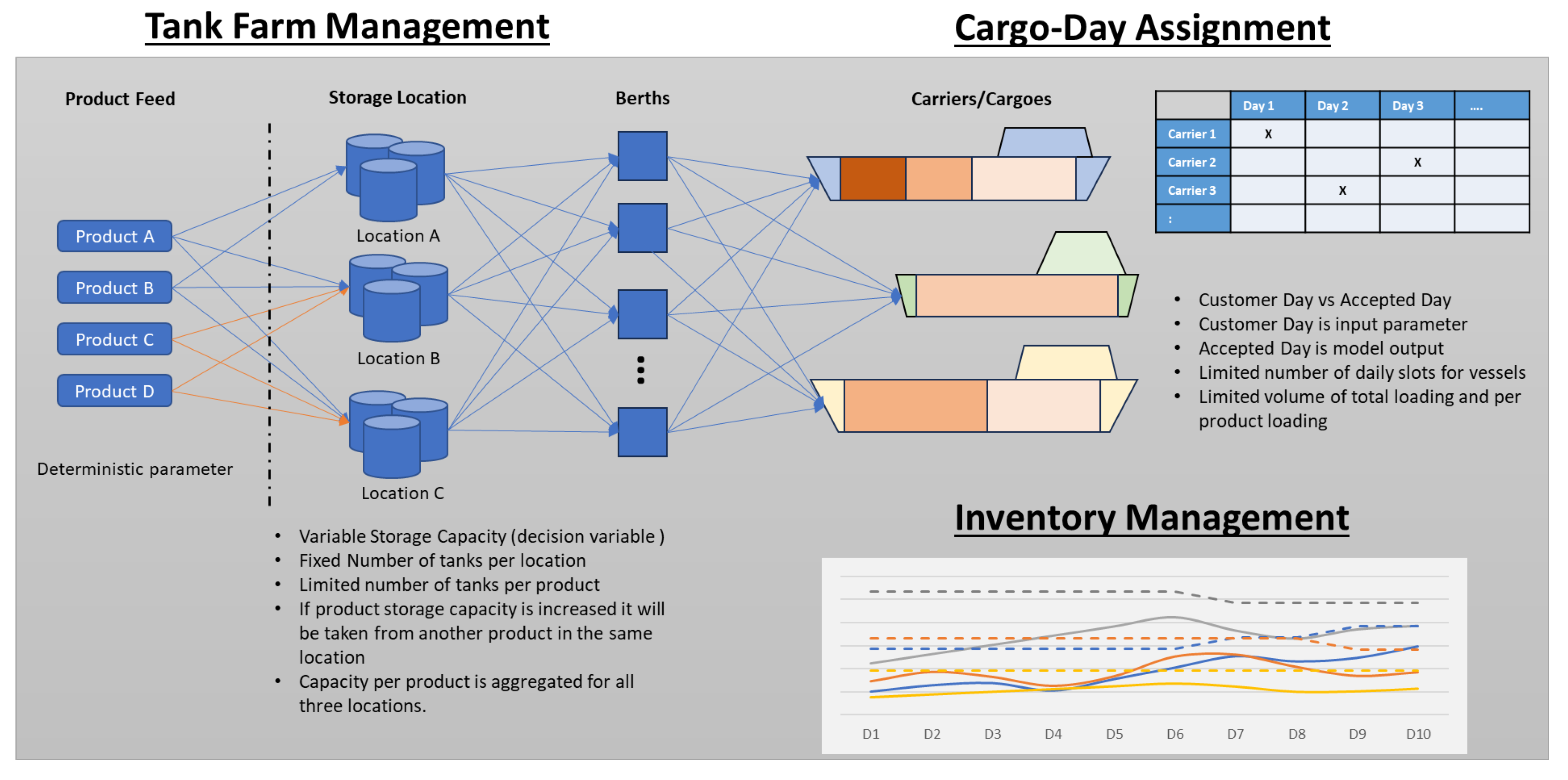
In this study, a mixed-integer programming (MIP) model for Crude Oil Terminal Scheduling (COTS) is formulated. The model extends our earlier work [5] by incorporating multiple objectives to better reflect real-world multi-criteria decision-making scenarios. The proposed model is a dynamic, multiproduct (different grades of crude oil), single-location inventory model that is efficiently integrated into oil carrier scheduling. It schedules oil carriers so that specific quantities of designated products (contractual commitments) are loaded on optimal loading dates. These optimal dates are determined by the model as a result of the trade-off between customers’ preferred dates and the nearest feasible loading dates. Several capacity constraints are considered at the terminal, including the number of berths available for simultaneous vessel service, tank storage capacities, the limited number of tanks that can switch product, and the availability of each crude oil grade.

The rest of this paper is arranged as follows: We offer a review of the published literature in the next section that addresses scheduling, inventory management, and/or optimization in the crude oil shipping industry. In Section 3, we introduce typical operations at crude oil terminals and break down their systems into individual components. In Section 4, the COTS assumptions and the MIP model are presented, along with the notations, including parameters and variables. Furthermore, the components of the mathematical model are presented in this section. In Section 5, we present different approaches to handle multiple objectives. Specifically, we exploit a lexicographic ordering of the objectives and then solve the models using a hierarchical optimization approach as well as a weighted Tchebycheff approach. Section 6 presents the validity of the presented model through a case study. The results are presented to demonstrate the pertinence of the proposed model. Additionally, a comparative discussion between the weighted sum approach and the Pareto generating approaches is presented in this section. Finally, the key achievements of the work and future research directions are depicted in Section 7.

2. Literature Review

To the best of the authors’ knowledge, the COTS problem has received limited attention in the oil and gas supply chain literature. Existing studies in the literature primarily address berth allocation in the marine supply chain, vessel routing, pipeline scheduling, and refinery scheduling (Table 1). The studies also propose various optimization models and methodologies to improve efficiency and overcome operational complexities.

The study of berth and ship dispatching scheduling has advanced significantly through methodologies like those of Golias et al. [6], who introduced a robust approach using hierarchical optimization and genetic algorithms to tackle discrete berth scheduling problems. Bausch et al. [7] complemented this by developing a mathematical programming model that optimizes ship dispatch schedules, enhancing both timelines and resource utilization. In vessel assignment and inventory management, Ye et al. [8] presented a two-level model assigning vessels to tasks based on product and destination requirements while avoiding operational overlaps, and Misra et al. [9] formulated a maritime inventory routing problem using an MILP model to optimize supply systems via efficient ship movements and jetty allocations.

Pipeline scheduling and inventory management have been thoroughly researched by Relvas et al. [10] and Castro et al. [11], who focused on MILP models for tank farm inventory management and pipeline scheduling, maintaining safe inventory levels and optimizing product sequences to meet demand while minimizing undesirable intermixing. Zheng et al. [12] introduced a model for optimizing crude oil procurement integrated with blending operations in refineries, utilizing a hybrid event–continuous-time model to effectively manage time scales, reduce procurement costs, and ensure stability in blended crude oil properties.

In crude oil scheduling, Zhang et al. [13] developed a dual-stage evolutionary algorithm, enhancing performance through a global search and local refinement, while Wang et al. [14] refined the multi-operation sequencing model, improving computational efficiency and solution quality in marine-access refineries. Advanced scheduling techniques have been proposed by Zhang et al. [15], who developed a Variable-Length Constrained Evolutionary Algorithm (VLCEA), and Zimberg et al. [16], who formulated a continuous-time approach for multi-operation sequencing, resulting in high-quality solutions for crude oil operations.

Efficient scheduling of crude oil operations has also been addressed by Yang et al. [17] through a rolling horizon approach and Zhang et al. [18] with a multi-scale strategy and multi-criteria optimization model for monthly refinery operations. Integrated optimization approaches by Yu et al. [19] and clustering-based methods by Assis et al. [20] have further reduced computational efforts in operational management.

Heuristic methods for operational management have been explored by An et al. [21] in vessel and port operation scheduling, highlighting cost savings and transportation optimization, and Assis et al. [22] in integrating crude oil supply management from offshore production to refining. Practical approaches for chemical tanker scheduling have been presented by Cankaya et al. [23], while Yamashita et al. [24] proposed a multi-start heuristic method for ship routing and scheduling, providing effective solutions for maritime logistics. Yang et al. [25] designed a multimodal transport network to optimize the use of energy resources and enhance the stability of the energy system, thereby improving energy security. They converted the problem into a nonlinear and multi-objective assignment problem of transportation optimization. Lv et al. [26] very recently provided a review of the literature on optimization methods in scheduling, particularly for port operations, covering quay crane scheduling, tugboat scheduling, pilot assignment, berth allocation, and channel-constrained vessel scheduling.

Optimization systems for pipeline planning were developed by Quinteros et al. [27], and a novel MINLP model for inland refinery crude scheduling was introduced by Qu et al. [28]. Panda et al. [29] proposed a reactive scheduling methodology using a structured, adapted genetic algorithm to handle uncertainties in marine-access refineries. Iterative decomposition methods for pipeline scheduling have been explored by De Assis et al. [30], while Zhang et al. [31] addressed crude oil operations in inland refineries through a continuous-time MINLP model, effectively managing long-distance pipeline transportation challenges.

Risk assessment in crude oil transportation has been highlighted by Siddiqui et al. [32], who developed a framework balancing economic efficiency and environmental protection through optimized crude oil tanker routing and scheduling. Zimberg et al. [33] focused on optimizing crude oil terminal operations with an MILP model and a rolling horizon strategy. In contrast, Hennig et al. [34] compared continuous and discrete cargo models for tanker routing and scheduling. Recently, Yang et al. [35] introduced a quantitative regional risk model to assess both individual and societal risks in oil tank farms, with a major focus on energy-related risks, including fires, leaks, and explosions. To provide an accurate and comprehensive evaluation of regional risks, their model integrated various factors, including weather conditions, operational variations in day–night operations, and risk superposition.

Strategic and tactical decision-making in the crude oil supply chain has been systematically reviewed by Sahebi et al. [36], who emphasized the need for advanced solution techniques. Transportation and inventory scheduling models have been addressed by De Assis et al. [37] and Yongtu et al. [38], who developed an MINLP model and simulation software for multiproduct pipeline delivery schedules. Integrated refinery scheduling, combining production scheduling with unit operation optimization, was demonstrated by Robertson et al. [39] to be beneficial in considering both logistical and operational costs.

Dynamic scheduling for refinery operations has been proposed by Yuzgecc et al. [40] using an MPC-based approach, while Rocha et al. [41] and Cafaro et al. [42] developed MILP models for petroleum allocation and dynamic scheduling for multiproduct pipelines, respectively. Maritime transport optimization has been explored by Al-Eisa et al. [43] using MILP models and by Lasschuit et al. [44] and Neiro et al. [45] through supply chain development and operational planning in the petroleum industry using MINLP and MILP models. Finally, Aires et al. [46], Cafaro et al. [47], and Rejowski et al. [48] introduced MILP and continuous-time models for pipeline scheduling, with Pinto et al. [49] applying nonlinear and mixed-integer optimization models for short-term refinery scheduling with time-dependent conditions.

Table 1. Summary of related works in oil and gas supply chain scheduling.

Research Focus	Methodology/Model Type	Studies
Berth Allocation and Vessel Dispatching	Hierarchical optimization, genetic algorithm, MILP, multilayer perceptron	[6,7,50]
Vessel Assignment and Maritime Inventory Routing	Two-level MILP, maritime inventory routing, fractional programming	[8,9,51]
Pipeline Scheduling and Tank Farm Inventory Management	MILP, MINLP, iterative decomposition, continuous-time modeling	[10,11,27,28,30,31]
Crude Oil Scheduling and Refinery Operations	Evolutionary algorithms, MILP, continuous-time optimization, rolling horizon	[13,14,15,16,17,18]
Integrated Optimization and Heuristic Approaches	Heuristic optimization, MILP, MINLP, multiobjective optimization, clustering methods	[19,20,21,22,23,24,25,26]
Risk and Safety in Crude Oil Operations	Bi-objective optimization, MILP, continuous/discrete models, risk assessment modeling, simulation	[32,33,34,35,52]
Strategic and Tactical Supply Chain Planning	MINLP, simulation modeling, integrated scheduling	[36,37,38,39]
Dynamic Refinery Scheduling and Petroleum Allocation	MPC-based control, MILP, MINLP, nonlinear optimization, continuous-time models	[40,41,42,43,44,45,46,47,48,49]

Table 1. Summary of related works in oil and gas supply chain scheduling.

Research Focus	Methodology/Model Type	Studies
Berth Allocation and Vessel Dispatching	Hierarchical optimization, genetic algorithm, MILP, multilayer perceptron	[6,7,50]
Vessel Assignment and Maritime Inventory Routing	Two-level MILP, maritime inventory routing, fractional programming	[8,9,51]
Pipeline Scheduling and Tank Farm Inventory Management	MILP, MINLP, iterative decomposition, continuous-time modeling	[10,11,27,28,30,31]
Crude Oil Scheduling and Refinery Operations	Evolutionary algorithms, MILP, continuous-time optimization, rolling horizon	[13,14,15,16,17,18]
Integrated Optimization and Heuristic Approaches	Heuristic optimization, MILP, MINLP, multiobjective optimization, clustering methods	[19,20,21,22,23,24,25,26]
Risk and Safety in Crude Oil Operations	Bi-objective optimization, MILP, continuous/discrete models, risk assessment modeling, simulation	[32,33,34,35,52]
Strategic and Tactical Supply Chain Planning	MINLP, simulation modeling, integrated scheduling	[36,37,38,39]
Dynamic Refinery Scheduling and Petroleum Allocation	MPC-based control, MILP, MINLP, nonlinear optimization, continuous-time models	[40,41,42,43,44,45,46,47,48,49]

In this study, we address the tactical-level scheduling decisions made daily at crude oil terminals. The main decisions that are made include scheduling oil carriers, managing tank inventories, and limiting service changes in the storage tanks. Further, all these decisions are made through the COTS model proposed in this work. The immediate objectives are to minimize the maximum and total deviation between the berth assignment date and the customers’ preferred loading date. The secondary objectives are to minimize the number of tank service switches and minimize the events when the inventory violates the soft constraint limits. To address multiple objectives, in this work, several solution approaches, namely the weighted sum approach, the hierarchical optimization approach, and the Tchebycheff approach, are developed.

3. Crude Oil Terminal Operation

There are two types of crude oil terminal systems (COTs): onshore and floating marine terminals. Each one has its own advantages and disadvantages; however, they both have the same logistics and operations from a scheduling point of view [53]. The crude oil terminal system consists of

• Feed lines, supplying product to the terminal.
• Storage tanks and water handling units.
• Loading systems, supplying products from tanks to ships.
• Berths, where a ship can be secured and load the product.

The crude oil terminal operations are

• Crude Receiving: Crude oil is supplied to the terminal through pipelines, and depending on the infrastructure of the facility and the supplier capability, the terminal can receive multiple products simultaneously or a single product at a time [53].
• Crude Storage: Crude oil is stored in crude tanks, and their capacity corresponds to the expected production rate to operate the terminals safely and to reduce product-handling costs. The number of tanks is allocated for a specific product to optimize its expected turnover. Also, some tanks can only handle a limited number of products out of the available ones due to infrastructure limitations [53].
• Crude Settling: Usually, crude arrives at the terminal with associated water. As soon as the crude is stored safely, oil–water separation by gravity starts in the tanks. After several hours, excessive water is then collected from the tanks in a water collection pond or sent to the oily water processing unit [53].
• Crude Loading: Upon crude carrier arrival at the terminal, and after finishing administrative work such as documentation, inspection, and verification, cargo hoses are connected to the carrier to start loading its cargo from the tanks. Additionally, the rate at which cargo is loaded into the carrier depends on the terminal’s available pumping capacity. Moreover, crude carriers come in different sizes and may load single or multiple cargoes based on the customer’s requirements. Terminals are committed to loading the cargoes in a timely manner to avoid demurrage and operation interruption [53]. Ships receive their cargo through a loading system, which is a collection of pumps and pipes that supply cargoes to the carriers. Usually, each loading system is used for a single product; otherwise, the pipeline must be flushed before using the system for another product.

4. Mathematical Model on Crude Oil Terminal Scheduling (COTS)

The proposed model is an extension of the previously proposed model presented in [5], where an allocation model used to plan oil carriers was developed and solved as a single-objective model. In these models, the problem will have a discrete-time representation, i.e., each day will be represented as a single time slot that can serve a number of oil carriers. The following subsection presents the assumptions for the development of the model.

4.1. Assumptions

• The total demand, including the opening inventory, is assumed to be less than the available supply.
• Backorders are not permitted; thus, inventory levels must remain non-negative at all times.
• The inventory is aggregated by the product pool across all terminal locations.
• The scheduled numbers of carriers per day are restricted to half the number of available berths, thereby preventing berth overlap in cases where loading operations extend beyond a single day.
• The impact of variations in loading capacity between two successive days is assumed to be negligible (Figure 3).

4.2. Model Formulation

The proposed COTS model is formulated using a structured set of indices, parameters, and decision variables.

Table 2. Definition of indices and sets.

Symbol	Description
i	Index of crude carriers, where $i\in I=\{1,2,\dots ,n\}$, and n represents the total number of crude carriers within the planning horizon.
j	Index of days, where $j\in J=\{1,2,\dots ,d\}$, and d denotes the total number of days in the planning horizon.
k	Index of products, where $k\in P=\{1,2,\dots ,p\}$, and p indicates the total number of products.
l	Index of locations, where $l\in M=\{1,2,\dots ,m\}$, and m is the total number of tank farms.

defines the sets and indices that represent the fundamental entities involved in the problem.

Table 3. Definition of parameters.

Symbol	Description
$D_j$	The jth day in the planning horizon (for $j\in J$).
$N_i$	The ith carrier’s preferred loading day (for $i\in I$).
$C_{ik}$	The cargo size (in cargoes) of the kth product to be loaded on the ith carrier (for $i\in I$ and $k\in P$).
$P_{ik}$	Binary parameter indicating whether the ith carrier requests the kth product: $$P_{ik}=\left\{\begin{array}{cc}1,\hfill & \mathrm{if}\mathrm{the}i\mathrm{th}\mathrm{carrier}\mathrm{requests}\mathrm{the}k\mathrm{th}\mathrm{product},\hfill \\ 0,\hfill & \mathrm{otherwise}.\hfill \end{array}\right.$$
$P{M}_{jk}$	The maximum number of cargoes (in cargoes) of the kth product that can be loaded on the jth day.
$Avrg{C}_k$	The average cargo size (in barrels) for the kth product.
$O{I}_{jk}$	The opening inventory of the kth product on the jth day (in barrels).
$F_{jk}$	The quantity of the kth product fed to the terminal on the jth day (in barrels).
$S_j$	The maximum number of carriers that can be scheduled on the jth day.
$Q{C}_j$	The maximum loading capacity (in barrels) for the crude oil terminal for the jth day.
$Avg{T}_{kl}$	The average tank size (in barrels) for the kth product at the lth location.
$Max{T}_{kl}$	The maximum number of tanks that can store the kth product at the lth the location.
$ATank{s}_{jl}$	Number of tanks available on the jth day at the lth location.
$P{r}_i$	The priority level of the ith carrier; a higher value indicates lower deviation from the requested date.
w	The penalty coefficient for changing tank service.
$cr$	The penalty coefficient for violating soft inventory limits.

summarizes the model parameters, which describe system characteristics, operational capacities, and penalty factors.

Table 4. Decision variables.

Symbol	Description
$x_{ij}$	Binary variable indicating whether the ith crude carrier is scheduled on the jth day: $$x_{ij}=\left\{\begin{array}{cc}1,\hfill & \mathrm{if}\mathrm{the}i\mathrm{th}\mathrm{carrier}\mathrm{is}\mathrm{scheduled}\mathrm{on}\mathrm{the}j\mathrm{th}\mathrm{day},\hfill \\ 0,\hfill & \mathrm{otherwise}.\hfill \end{array}\right.$$
$t_{jkl}$	Total number of tanks in tank farm l that store product k on the jth day.
$r_{jk}^{+}$	Total volume of product k exceeding the soft maximum inventory limit on the jth day.
$r_{jk}^{-}$	Total volume of product k below the soft minimum inventory limit on the jth day.
$y_i^{+}$	Linearization variable representing the absolute deviation of the ith carrier from its requested loading day.
$q_{jk}$	Total volume of product k loaded on the jth day.
$c_{jk}^s$	Available storage capacity for product k on the jth day.
$I_{jk}$	Inventory level of product k on the jth day.
${\mu }^{+}$	Maximum allowable delay (in days) for scheduling a carrier.
${\mu }^{-}$	Maximum allowable advancement (in days) for scheduling a carrier.
${\theta }_{jkl}$	Number of tank service changes for product k at location l between the jth and $(j-1)$th days.
${\theta }_{jkl}^{+}$	Absolute number of tank service changes for product k at location l between the jth and $(j-1)$th days.

details the decision variables that govern scheduling, allocation, and inventory decisions within the optimization framework.

• Next, the mathematical model is presented:

• Objective Function:

$$Min.:\left\{{\mu }^{+}+{\mu }^{-};\sum _{i\in I}P{r}_i\ast y_i^{+};\sum _{\begin{array}{c}l\in M\\ k\in P\\ j\in J\end{array}}{\theta }_{jkl}^{+};\sum _{\begin{array}{c}k\in P\\ j\in J\end{array}}(r_{jk}^{+}+r_{jk}^{-})\right\}$$

(1)

Constraints:

$$\sum _{j=1}^d{x}_{ij}\ast D_j-N_i\le y_i^{+}\mathrm{and}{N}_i-\sum _{j=1}^d{x}_{ij}\ast D_j\le y_i^{+}\forall i$$

(2a)

$$\sum _{j=1}^d{x}_{ij}\ast D_j-N_i\le {\mu }^{+}\forall i$$

(2b)

$$N_i-\sum _{j=1}^d{x}_{ij}\ast D_j\le {\mu }^{-}\forall i$$

(2c)

$$\sum _{j=1}^d{x}_{ij}=1\forall i$$

(2d)

$$q_{jk}=\sum _{i=1}^n{x}_{ij}\ast C_{ik}\forall j,k$$

(2e)

$$I_{jk}=O{I}_{jk}+F_{jk}-q_{jk}\forall j=1 \& \forall k$$

(2f)

$$I_{jk}=I_{j-1,k}+F_{jk}-q_{jk}\forall j\ge 2 \& \forall k$$

(2g)

$$I_{jk}\le c_{jk}^s\forall j,k$$

(2h)

$$I_{jk}\ge 0\forall j,k$$

(2i)

$$I_{jk}\le 0.8\ast c_{jk}^s+r_{jk}^{+}\forall j,k$$

(2j)

$$I_{jk}\ge 3\ast Avrg{C}_k-r_{jk}^{-}\forall j,k$$

(2k)

$$\sum _{i=1}^n{x}_{ij}\le S_j\forall j$$

(2l)

$$\sum _{i=1}^n{x}_{ij}\ast P_{ik}\le P{M}_{jk}\forall j,k$$

(2m)

$$\sum _{k=1}^p{q}_{jk}+q_{j+1,k}\le Q{C}_j+Q{C}_{j+1}\forall j$$

(2n)

$$c_{jk}^s=\sum _{l=1}^m{t}_{jkl}\ast Avg{T}_{kl}\forall j,k$$

(2o)

$$t_{jkl}\le Max{T}_{kl}\forall j,k,l$$

(2p)

$$\sum _{k=1}^p{t}_{jkl}=ATank{s}_{jl}\forall j,l$$

(2q)

$${\displaystyle \frac{t_{jkl}-t_{j-1,kl}}{2}}={\theta }_{jkl}\forall j,k,l$$

(2r)

$${\theta }_{jkl}\le {\theta }_{jkl}^{+}and-{\theta }_{jkl}\le {\theta }_{jkl}^{+}\forall j,k,l$$

(2s)

$$\begin{array}{c}\hfill x_{ij}\in \{0,1\},\forall i,j,\\ \hfill t_{jkl}\in {\mathbb{Z}}_{+},{\theta }_{jkl}\in \mathbb{Z},\forall j,k,l,\\ \hfill r_{jk}^{+},r_{jk}^{-},y_i^{+},q_{jk},c_{jk}^s,I_{jk}\ge 0,\forall j,k,\\ \hfill {\mu }^{+},{\mu }^{-}\ge 0,\\ \hfill {\theta }_{jkl}^{+}\ge 0,\forall j,k,l.\end{array}$$

(2t)

4.2.1. Linearized Deviation from Preferred Loading Day

The deviation from the requested loading day is given as

$$|\sum _{j=1}^d{x}_{ij}\ast D_j-N_i|\forall i$$

(3)

Equation (3) can be linearized by introducing variables $y_i^{+}\ge 0$ for $i=1,\dots ,n$, as shown in Equation (2a). Equations (2b) and (2c) set upper and lower limits on the maximum number of days that an oil carrier can deviate. Equation (2d) ensures that each carrier is assigned to exactly one loading day.

4.2.2. Inventory Balance and Capacity

Equation (2e) estimates the total quantity of product k loaded on day j. Equations (2f) and (2g) illustrate the inventory balance constraints. Moreover, Equations (2h) and (2i) set hard constraints related to the physical storage capacity, where the storage capacity for product k on day j is dynamically changed, as shown in Equation (2o).

On the other hand, we also consider soft constraints on the physical storage. The idea is to penalize any inventory level beyond 80% of the available storage capacity. Equation (2j) implements this idea of a soft max capacity constraint. Similarly, Equation (2k) corresponds to the soft min constraint. The idea is to maintain an inventory level at least three times the average cargo size of product k, during the planning horizon, where the average cargo size $Avrg{C}_k$ is estimated as shown in Equation (4).

$$Avrg{C}_k={\displaystyle \frac{{\sum }_{i=1}^n{C}_{ik}}{{\sum }_{i=1}^n{P}_{ik}}}.$$

(4)

4.2.3. Terminal and Loading Capacities

Due to the terminal and carrier size, there is a limitation on the number of carriers served on a single day. Equation (2l) limits the total number of carriers permitted to be scheduled for loading on a given day. Furthermore, each loading system is capable of handling a single product at any given time. The quantity of cargoes of the same product that can be loaded on the same day must be limited due to the available capacity of the loading systems. Equation (2m) restricts the number of payloads of the single product to be loaded on a single day.

Moreover, crude oil terminals load vessels through pipelines using pumps, with each loading line having a defined transfer capacity based on its size and pumping rate. Since large carriers typically require between one and two days to complete loading and the model operates on a discrete-time basis, the loaded quantities over two consecutive days must be monitored to ensure they remain within the combined loading capacity. This logic is implemented in Equation (2n).

4.2.4. Tank Farm Storage

In this dynamic framework, storage at the tank farms is treated as a controllable parameter that can be adjusted based on the daily allocation of storage tanks to specific crude oil products. The terminal consists of multiple tank farms, each characterized by distinct storage capacities, tank counts, and product-handling capabilities determined by the crude grades assigned to them. Equation (2o) dynamically determines the storage capacity allocated to product k on day j. Equation (2p) restricts the number of tanks allocated on day j to product k within the tank farm l. Finally, Equation (2q) guarantees that all available tanks are fully utilized.

4.2.5. Linearized Service Changes in Tanks

The system permits changes in tank service when necessary. However, such modifications are undesirable and should be minimized. Ideally, the modification may involve either adding or deducting a tank from the service of the given product k. Thus, the absolute value of ${\theta }_{jkl}$ can be represented as

$${\theta }_{jkl}={\displaystyle \frac{|t_{jkl}-t_{j-1,kl}|}{2}}\forall j,k,l$$

(5)

Equation (5) also accounts for potential double counting of service reassignments, since an increase in the number of tanks serving one product corresponds to a decrease for another, resulting in two counted changes for a single reassigned tank. To linearize this formulation, an auxiliary variable ${\theta }_{jkl}^{+}$ is introduced along with the following constraints: Equations (2r) and (2s).

5. Handling Multiple Objectives

In this section, we present different approaches for handling the multiple objectives. Specifically, we will focus on the weighted sum approach, the hierarchical optimization approach, and the weighted Tchebycheff approach.

5.1. Weighted Sum (WS) Approach

The WS objective function, shown in Equation (6), minimizes three components: the deviation from carriers’ requested loading dates, violations of inventory restrictions, and the number of tanks that change their service. Nevertheless, the objective in Equation (6) is not directly comparable across components, as each is expressed in different units. Specifically, the deviation component is measured in days, the tank service change component in the number of tanks, and the inventory violation component in volume.

$$MinZ=\sum _{i=1}^{n}P{r}_i\ast y_i^{+}+w\ast \sum _{l=1}^m\sum _{k=1}^p\sum _{j=1}^d{\theta }_{jkl}^{+}+cr\ast \sum _{k=1}^p\sum _{j=1}^d(r_{jk}^{+}+r_{jk}^{-})$$

(6)

The unification of the objective function can be achieved by transforming all three components to equivalent volume measures. This is achieved by multiplying the divergence in loading days by the carrier’s cargo capacity and by multiplying the average tank size of product k by the number of tanks that change service, as revealed in Equation (7).

$$\begin{array}{c}\hfill MinZ=\sum _{k=1}^p{C}_{ik}\ast \sum _{i=1}^{n}P{r}_i\ast y_i^{+}+w\ast \sum _{l=1}^m\sum _{k=1}^p\sum _{j=1}^{d}Avg{T}_{kl}\ast {\theta }_{jkl}^{+}\\ \hfill +cr\ast \sum _{k=1}^p\sum _{j=1}^d(r_{jk}^{+}+r_{jk}^{-})\end{array}$$

(7)

Even though the units are merged, the objective function given in Equation (7) inherently prioritizes carriers with larger volumes. This behavior is not aligned with the business requirements, as neither the carrier’s cargo volume nor the tank size should influence the prioritization of carriers or tanks.

Robust WS Approach to Handle Potential Infeasibility

In our initial attempts, the model was solved using Equation (7), with ${\mu }^{+}$ and ${\mu }^{-}$ as given parameters. After testing the initial model on several datasets, it was observed that not all carriers could be scheduled within the predefined deviation limits, ${\mu }^{+}$ and ${\mu }^{-}$. To address this issue, the model was modified to minimize the maximum delay and advancement by converting ${\mu }^{+}$ and ${\mu }^{-}$ into variables. Furthermore, they were directly added to the objective function. We apply a penalty $m^{+}$ for exceeding ${\mu }^{+}$, while a higher penalty $m^{++}$ is assigned for violating ${\mu }^{-}$, as advancing the loading date is typically unacceptable to customers. The resulting robust WS objective function is presented in Equation (8). A pseudocode depicting the robust WS approach is presented in Algorithm 1.

$$\begin{array}{c}\hfill MinZ=m^{+}\ast {\mu }^{+}+m^{++}\ast {\mu }^{-}+\sum _{i=1}^{n}P{r}_i\ast y_i^{+}\\ \hfill +\sum _{k=1}^p\sum _{j=1}^d(r_{jk}^{+}+r_{jk}^{-})\ast cr+(\sum _{l=1}^m\sum _{k=1}^p\sum _{j=1}^d{\theta }_{jkl}^{+})\ast w\end{array}$$

(8)

Algorithm 1: Pseudocode of the Weighted Sum (WS) Approach

Input: Constraint set from Equations (2) and objective functions from Equation (8). Output: Optimal Operating point for a given set of weights. Step 1: Select the suitable weights. Select values for $m^{+},m^{++},P{r}_i,cr,w$ based on decision-maker’s input. Step 2: Solve the WS model. Where the objective function is from Equation (8) and the constraint set is from Equations (2). returnBest solutions within 3000 secs.

5.2. Pareto Generating Approaches

In the field of decision-making, particularly in complex systems or procedures, we frequently come across circumstances that call for the simultaneous optimization of several competing goals. Rather than searching for a single ideal solution, multi-objective optimization seeks to identify a set of solutions that balance multiple goals. The Pareto front, or Pareto optimal set, is a useful concept in multi-objective optimization that illustrates the trade-offs between many objectives.

The proposed problem has multiple objectives to be solved simultaneously; the objective function in Equation (8) uses a single weighted objective to solve the multi-objective optimization model. The aim is to handle each individual objective separately. Finally, a Pareto front can be generated by altering the importance associated with each objective, as shown in Section 5.4.

There are several methods used to solve the multi-objective model for each objective. Examples of those methods include hierarchical optimization, the weighted Tchebycheff procedure, and goal programming. Here, the problem will be solved using the hierarchical optimization method in addition to using the weighted Tchebycheff procedure and then comparing their results with the single-weighted-objective approach.

5.3. Hierarchical Optimization (HO) Approach

A lexicographic order needs to be established for the set of objectives to make sure that the best outcome, aligned with the business requirements, is achieved. This ordering of the objectives will be further exploited via the HO modeling approach. According to the subject matter experts, minimizing the maximum deviation from the customer-requested loading date is preferred over reducing the deviation per shipment. With this, the first two objectives will be related to the shipment schedule. The remaining objectives are related to the tank farm operations in terms of managing the inventory and the storage capacity for all products. The subject matter experts stated that although it is applicable to change the service for a number of tanks, they would like to keep this to the bare minimum, even though that means violating the soft max and soft min inventory constraints. Thus, the third and fourth objectives will be minimizing the number of tank services switched and minimizing the violation of the soft constraint to exceed the soft limits of the inventory, respectively.

• The lexicographic order for the objectives is as follows:

• Objective 1: Minimizing the maximum days deviated. ${\mu }^{+}+10\ast {\mu }^{-}$.
• Objective 2: Minimizing the total days’ deviation from the requested loading date for each nomination. ${\sum }_{i=1}^n{y}_i^{+}\ast P{r}_i$.
• Objective 3: Minimizing the number of tank services switched. ${\sum }_{l=1}^m{\sum }_{k=1}^p{\sum }_{j=1}^d{\theta }_{jkl}^{+}$
• Objective 4: Minimizing the violation of the soft constraint to exceed the soft limits of the inventory. ${\sum }_{k=1}^p{\sum }_{j=1}^d(r_{jk}^{+}+r_{jk}^{-})$

• The same model constraints from Equations (2) will be used here with minor modifications. In order to present the modification, let us define the following set:

• $g:\mathrm{objective}\mathrm{index},g=1,2,3,4\mathrm{and}g\in Z$

• Additionally, the generic objective function given in Equation (1) will be broken into four constraints such that Objective 1 will be solved first, then Objective 2, then 3, and lastly Objective 4, and at each stage, the value of the previous objective will be introduced to the model as a constraint with a maximum deviation of ${ϵ}_g$. Each ${ϵ}_g$ is relative to the units and scale of each objective. The values of ${ϵ}_g$ based on our discussions with the subject matter experts are presented as follows:

• ${ϵ}_1$, which is related to the objective for the maximum deviation days and will be zero, since this is the most important objective, and it derives the supplier’s schedule quality.
• ${ϵ}_2$, which represents the additional days of deviation per shipment, and it will range from 1.5 to 2 days per shipment.
• ${ϵ}_3$, which is the additional number of tanks to change their service and will be 1.

• Finally, the set of new equations that will be added to the HO model is shown in Equation (9) to Equation (12), where ($z_1,\dots ,z_4$) are new variables added to the HO model.

$$z_1={\mu }^{+}+10\ast {\mu }^{-}$$

(9)

$$z_2=\sum _{i=1}^{n}P{r}_i\ast y_i^{+}$$

(10)

$$z_3=\sum _{l=1}^m\sum _{k=1}^p\sum _{j=1}^d{\theta }_{jkl}^{+}$$

(11)

$$z_4=\sum _{k=1}^p\sum _{j=1}^d(r_{jk}^{+}+r_{jk}^{-})$$

(12)

Finally, the model will loop over g, as shown in Algorithm 2. Since the values of ${ϵ}_g$ are fixed, the final model (last model in the loop) will give a single solution based on the business’s required preferences. However, if the subject matter experts’ information is not available, then a Pareto can be generated by selecting appropriate intervals for the values of ${ϵ}_g$ (also known as the $ϵ$ constraint approach). A pseudocode depicting the HO approach is presented in Algorithm 2.

Algorithm 2: Pseudocode of the Hierarchical Optimization (HO) Approach

5.4. Weighted Tchebycheff (WT) Approach

Here, another approach will be applied to the multi-objective optimization problem, which is the weighted Tchebycheff approach. The weighted Tchebycheff approach minimizes the weighted maximum deviation of a feasible solution to a desirable reference point. An alternative feasible solution will be produced by altering the selected weight for each objective, ultimately generating a Pareto feasible region [54].

Let $\mathcal{P}$ be the set of constraints containing all the constraints from Equation (2) and Equations (9) to (12). The feasible set $\mathcal{P}$ will be the basis of the WT procedure. Let the best achieved value for each individual objective be represented as $z_g^{\ast \ast }$; that is, $z_g^{\ast \ast }={\displaystyle \underset{\mathcal{F}}{min}}\left\{z_g\right\}$. Now, $z_g^{\ast \ast }$ is the desired reference point to be achieved by the corresponding objective. In addition to that, different weights $w_g$ are assigned for each objective such that ${\sum }_{g\in Z}{w}_g=1$. This will lead to the objective function, as depicted in Equation (13):

$$Z=\sum _{g\in Z}{w}_g\ast (z_g-z_g^{\ast \ast })$$

(13)

Scaling the objective function: Since the four objectives in the problem are not homogeneous, as they do not have the same scale nor unit of measure, scaling the objective function components to be between 0 and 1 is necessary to achieve balanced control over the multiple objectives. There are many methods to scale or normalize the data based on their bounds or distribution, such as linear scaling, as shown in Equation (14), or the z-score method, as illustrated in Equation (15).

$$z^{\prime }={\displaystyle \frac{z-z_{min}}{z_{max}-z_{min}}}$$

(14)

$$z^{\prime }={\displaystyle \frac{z-\mu }{\sigma }}$$

(15)

However, since there is no clear idea of the absolute bounds nor distribution of every objective, the linear scaling method shown in Equation (14) will be used. The $z_{min}$ value for each objective g will be equal to $z_g^{\ast \ast }$, and the value of $z_{max}$ will be $z_g^{++}$, which is assumed to be the maximum value of objective $z_g$ obtained while minimizing other objectives $z_{gg}$, $z_g^{++}=max\left\{z_g\right|{\displaystyle \underset{\mathcal{F}}{min}}{z}_{gg};gg\ne g\}$, or an appropriate upper bound based on the specific objective function based on the MIP relaxations. Thus, the scaled objective function will be

$$Z=\sum _{g\in Z}{w}_g\ast \left({\displaystyle \frac{z_g-z_g^{\ast \ast }}{z_g^{++}-z_g^{\ast \ast }}}\right)$$

(16)

The objective function introduced in Equation (16) is scaled between 0, when $z_g=z_g^{\ast \ast }$, and 1, when $z_g=z_g^{++}$. Hence, the solver will prioritize minimizing the objective with larger $w_g$, bringing it closer to the minimum achieved value $z_g^{\ast \ast }$ as intended. A pseudocode depicting the WT approach is presented in Algorithm 3.

Algorithm 3: Pseudocode of the Weighted Tchebycheff (WT) Approach

In the next section, we present a numerical case study, depicting the performance of the proposed WS, HO and WT approaches.

6. Case Study

In this section, the performance of the three proposed approaches is compared on a real-life case study. In this case study, we consider three tank farms with aggregated product pools, four different products, and a planning horizon of 30 days. The study involved multiple crude carriers to be scheduled at the terminal with a different cargo mix; the number of products in the same crude carrier is between 1 and 4 products and each cargo size varies from 0 to 2000 barrels. Additionally, each crude carrier has a different desired loading day. Furthermore, a daily feed rate to the terminal is provided for each product, based on the opening inventory, which is proportional to the demand. Along with all other loading capacity limitations, the quantity and capacity of the available storage tanks are also considered. The details of the parameters and their ranges are provided in

Table 5. Variable definitions, distributions, and units.

Parameter	Range/Distribution	Units
$D_j$	$U[10,90]$	days
$N_i$	$U[1,90]$	days
$C_{ik}$	$U[1,4]$	cargoes
$P_{ik}$	$B[0,1]$	binary
$P{M}_{jk}$	$U[0,20]$	cargoes
${\mathrm{AvrgC}}_k$	$U[100,2000]$	barrels
$O_{ijk}$	$U[0,{\mathrm{Cap}}_{jk}]$	barrels
$F_{jk}$	$U[0,{\mathrm{Cap}}_{jk}]$	barrels
$S_j$	$U[0,20]$	carriers
AvgTkl	$U[100,1000]$	barrels
MaxTkl	$U[0,100]$	tanks
$ATank{s}_{jl}$	$U[0,100]$	tanks
$Q{C}_j$	$U[0,{\mathrm{Cap}}_{jk}]$	barrels

. In the table, $U[A,B]$ implies a uniform random value between (and including) A and B.

These proposed mathematical models are modeled in GAMS 24.7.4 (https://www.gams.com/) and solved via CPLEX 12.6 (https://www.ibm.com/products/ilog-cplex-optimization-studio (accessed on 21 October 2025) solver. We set the terminating criteria for the solver as either reaching a relative tolerance of 1% from the best possible solution for WS and WT and 5% for HO, or reaching a time limit of 3000 s. The model is run on a system with an Intel Core Ultra 9 185H processor and 16 GB RAM.

6.1. Solving the Problem as a WS

The WS model returned a feasible solution in the time limit of 610 s and will be used to evaluate the performance of the other approaches, HO and WT.

6.2. Exploring Objective Function Values Using HO

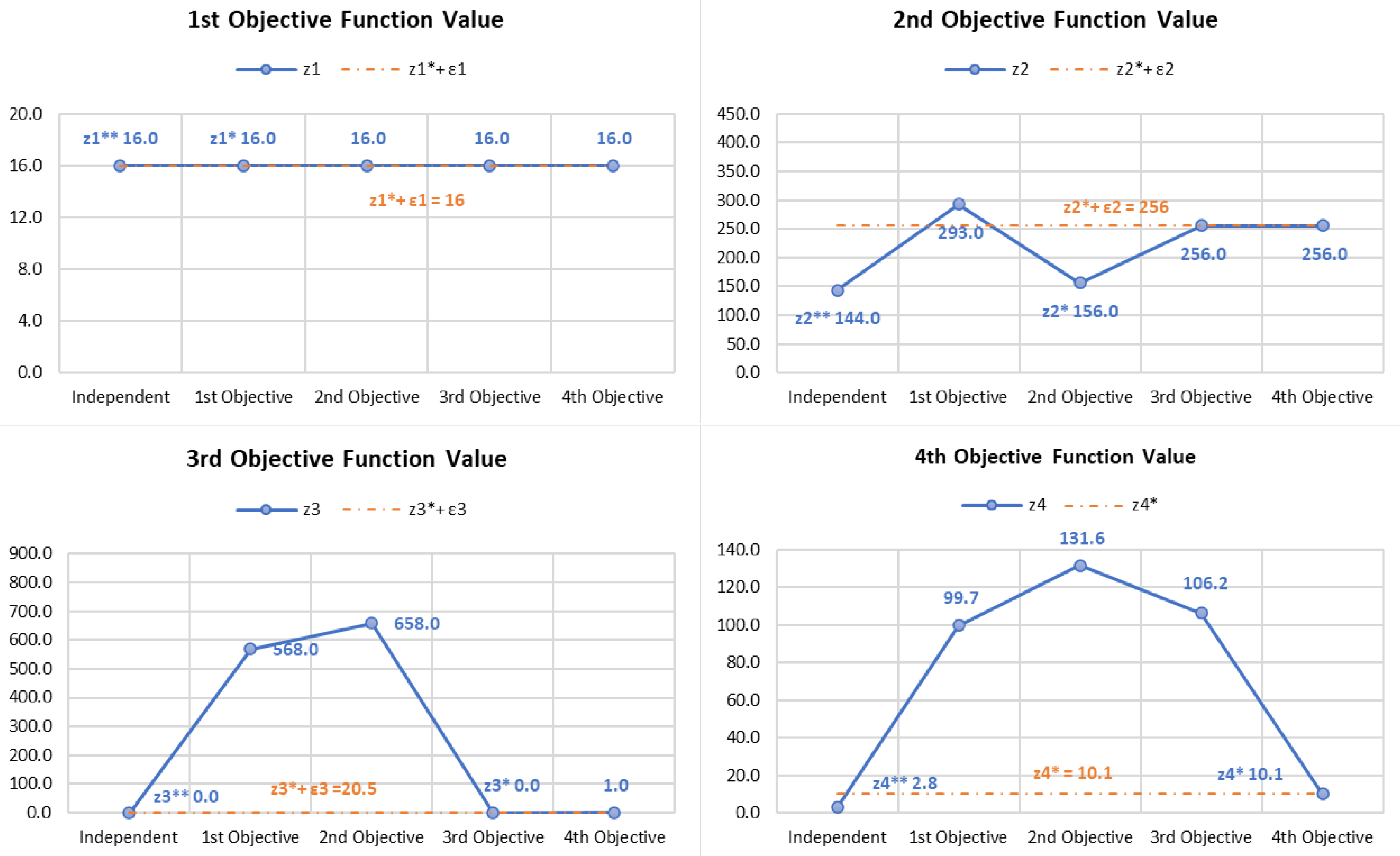
The hierarchical approach allows us to optimize each subordinate objective independently, hierarchically avoiding conflicts with other objectives. Figure 4 illustrates how each objective behaves on its own and shows that conflicting objectives stay within the allowable deviation of the $ϵ$ value.

We ran the model eight times to cover all possible scenarios. In four of these runs, we focused on minimizing each objective on its own. For the other four runs, we optimized the objectives with the $ϵ$ constraint based on the hierarchy among the objectives. This thorough analysis helped us understand the trade-offs between different objectives and their sensitivity. These insights are valuable for making informed decisions and finding the best strategies for this COTS.

6.3. Generating Pareto Fronts of Feasible Solutions Using WT

Every non-dominated solution, or the points where no other solution simultaneously achieves better results in any of the objectives, makes up the Pareto front. This is similar to determining the ideal point at which achieving one goal cannot come at the expense of another. To produce the Pareto front, the model is solved multiple times with different $w_g$ at each run. For this problem, the model is solved five times, and the weights are shown in

Table 6. Weight values for each run.

Case	${\mathit{w}}_1$	${\mathit{w}}_2$	${\mathit{w}}_3$	${\mathit{w}}_4$
1st	0.25	0.25	0.25	0.25
2nd	0.5	0.3	0.15	0.05
3rd	0.3	0.5	0.15	0.05
4th	0.15	0.05	0.5	0.3
5th	0.05	0.15	0.3	0.5

. Additionally, the relative values for each objective are shown in

Table 7. Relative objective’s values.

Case	${\mathit{z}}_1$	${\mathit{z}}_2$	${\mathit{z}}_3$	${\mathit{z}}_4$
1st	0%	10%	0%	5%
2nd	0%	8%	0%	12%
3rd	0%	8%	0%	8%
4th	0%	11%	0%	5%
5th	21%	10%	0%	3%

, and they are scaled using the values shown in

Table 8. Scaling values.

z	${\mathit{z}}_1$	${\mathit{z}}_2$	${\mathit{z}}_3$	${\mathit{z}}_4$
$z^{\ast \ast }$	16.0	144.0	0.0	2817.1
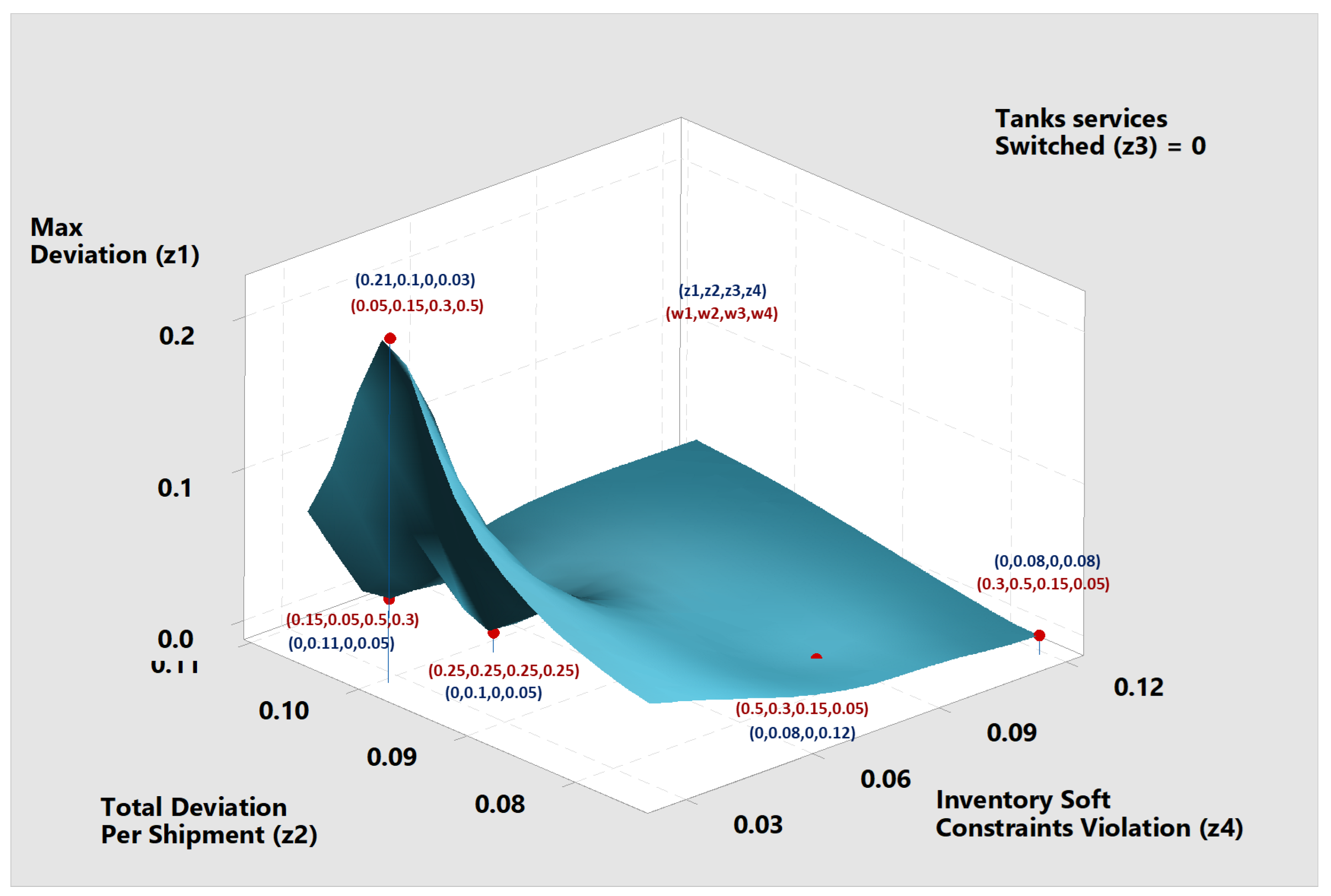
$z^{++}$	30.0	1341.0	658.0	131,560.2

, which are produced using HO. Interestingly, Objective 3 ($z_3$) is found to always hit the minimum value of $z_g^{\ast \ast }$; hence, it enables the generation of a 3D Pareto front, as shown in Figure 5, despite there being four objectives to be optimized.

6.4. Sensitivity Analysis

In order to evaluate the influence of key operational parameters, namely loading capacity, the number of daily time slots, and the number of available tanks, a sensitivity analysis is performed. Specifically, six scenarios are designed, as summarized in

Table 9. Summary of base and sensitivity scenarios.

Scenario ID	Description
S0	Base Scenario: Represents the baseline configuration used for comparison. All parameters remain at their nominal values.
S1	Scenario-1 tests the impact of increasing the loading capacity by 500 units, which may reduce congestion or improve scheduling flexibility.
S2	Scenario-2 evaluates the effect of reducing the loading capacity by 500 units, potentially stressing the system and increasing delays.
S3	Scenario-3 adds one berth or loading operation slot to assess improvements in throughput and scheduling efficiency.
S4	Scenario-4 removes one berth or loading slot to examine the system’s robustness under tighter scheduling constraints.
S5	Scenario-5 introduces one extra tank to test how increased storage capacity affects inventory balance and service flexibility.
S6	Scenario-6 reduces the number of available tanks by one to explore how limited storage impacts scheduling and delays.

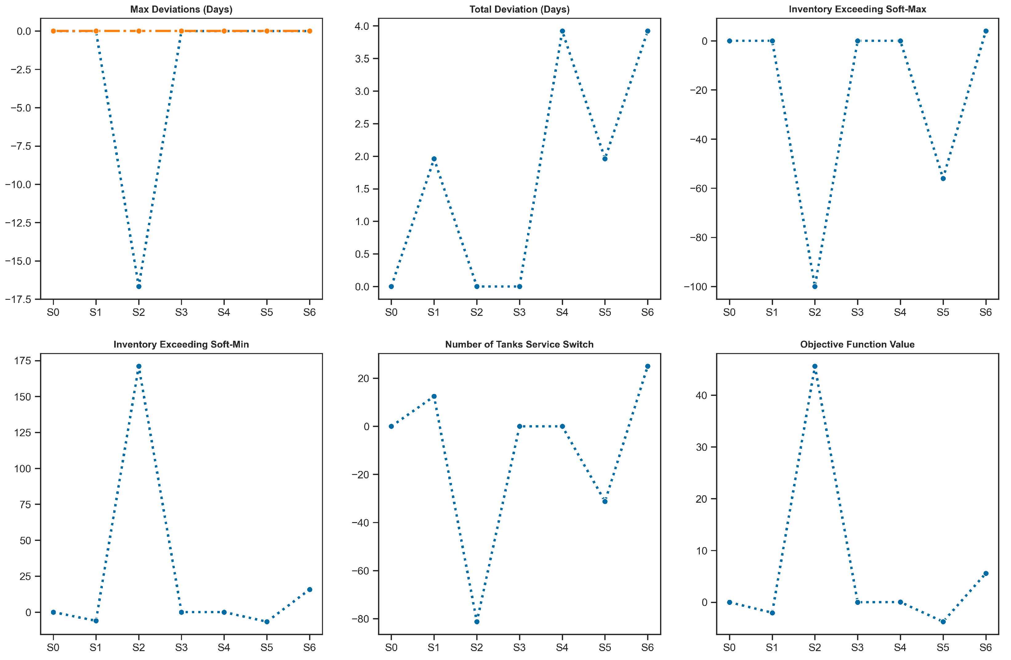
. The parameter values for these scenarios are generated based on the data provided in Table 5. All cases are solved to optimality using the CPLEX solver on the same computational setup described at the beginning of Section 6. Figure 6 provides an overview of the sensitivity analysis, in which the y-axis reports each scenario’s percentage change from the base scenario.

For each scenario, several performance indicators are analyzed:

Max deviations (days): This indicator represents the maximum deviation from the preferred loading date, including both delays (blue profile) and advancements (orange profile). The results indicate that none of the scenarios cause advancements in loading dates. However, Scenario S2 shows a noticeable decrease in maximum delays, suggesting that loading capacity has a significant effect on this measure.

Total deviations (days): Depicted in the top-middle subplot, this metric represents the total number of delayed days across the planning horizon. The results show that Scenarios S4 and S6 lead to substantial increases in total delays, highlighting the sensitivity of the schedule to daily slot and tank availability.

Inventory exceeding soft max: The top-right subplot illustrates the total inventory volume exceeding the soft maximum threshold (80% of the maximum level). The results indicate that Scenario S2 considerably reduces excess inventory, implying a more balanced inventory profile under this condition.

Inventory exceeding soft min: The bottom-left subplot shows the inventory volume going above the safety stock (calculated as three times $Avrg{C}_k$ during the planning horizon). Scenario S2 again has a pronounced effect, causing inventory levels to drop further below the soft minimum, which may reflect tighter operational constraints.

Number of tank service switches: This indicator, shown in the bottom-middle subplot, measures the frequency of tank service switches, where lower values are preferred. Scenario S2 significantly reduces this number, suggesting improved operational stability.

Objective function value: Illustrated in the bottom-right subplot, this value (computed using Equation (8)) represents the overall system performance. Scenario S2 exhibits the largest improvement in the objective function, confirming its strong impact on system efficiency.

In summary, Scenario S2, which corresponds to a reduction of 500 units in loading capacity, exhibits the most pronounced influence across all key performance indicators. Although Scenario S2 has a positive effect on max deviations, total deviations, the inventory exceeding soft max, and number of tank service switches, it performs very poorly with respect to the objective function value as well as the inventory exceeding soft min. Furthermore, Scenario S5, which corresponds to an increment in tanks by 1 unit, shows promising results with respect to all the performance indicators. This finding underscores the critical roles of loading capacity and number of tanks in determining overall system performance.

6.5. Result Comparison

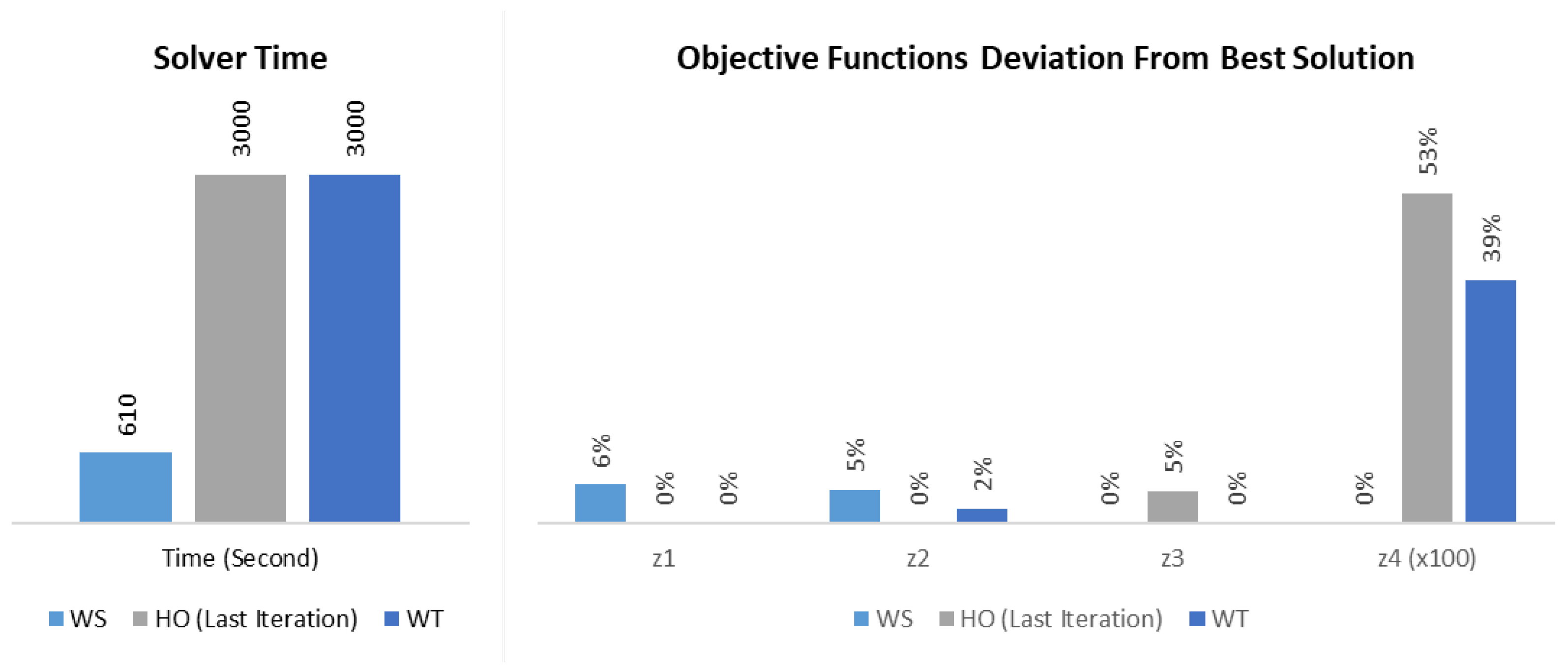
The three models’ results are compared in this section: WS, HO, and WT. For WT, we choose Case 1, where all $w_g$ are equal, to be used in this comparison. Figure 7 illustrates the time required to produce the results for each model along with the values of the four objectives for the three models.

The WS model dominated the other two in the time required to solve the problem, with one iteration that required 610 s to be solved, against multiple iterations for the HO and WT, some of which took up to 3000 s. Moreover, the HO and WT approaches produced better solutions compared to the WS method in alignment with the prioritization of business objectives.

Table 10. Best objective achieved.

z	${\mathit{z}}_1$	${\mathit{z}}_2$	${\mathit{z}}_3$	${\mathit{z}}_4$
WS			x	x
HO	x	x
WT	x		x

indicates which model produced the best value for each objective. Additionally, when comparing the best objectives from the HO and WT methods with the WS method, a marginal improvement is noticed.

Managerial Insights

For managers and decision-makers, understanding the Pareto region is valuable. It allows them to explore different trade-offs, assess robustness, and make informed choices. We can infer from the Pareto in Figure 5 that Objective 1, minimizing the maximum deviation days, is very robust and achieved the best found solution in four out of the five explored cases. Additionally, Objective 2, which aims to minimize the total days deviated, exhibits stability throughout all five scenarios with no apparent fluctuation, as the best attained value in this objective is 8%, while the worst is 11%, with a mere 3% gap between them. Moreover, Objective 3, minimizing the number of tank services switched, has no significant impact on the overall problem, as it always hits its best achieved solution in all explored cases. Furthermore, Objective 4, minimizing the inventory soft constraint violations, is very sensitive to the assigned weight and can be easily manipulated in case there is a need.

Analyzing the objectives’ behaviors, there is a clear trade-off between Objectives 3 and 4 and Objectives 1 and 2, as illustrated in Figure 6. The decision-maker needs to prioritize maintaining the number of tank service switches and the inventory below the soft constraint or minimizing the number of days deviated and maximizing customer satisfaction.

Finally, the decision-maker needs to understand the trade-off between the time required to solve each model and the generated solution. If time is of the essence, then the decision-maker may opt to use the WS method; otherwise, the HO or WT can produce more controlled results based on the objective priorities.

6.6. WT Solution

In this section, we illustrate the results of the WT method, exploring inventory profiles, product loading, crude carriers’ loading day distribution, and loading day deviation from the requested day.

6.6.1. Inventory Profiles

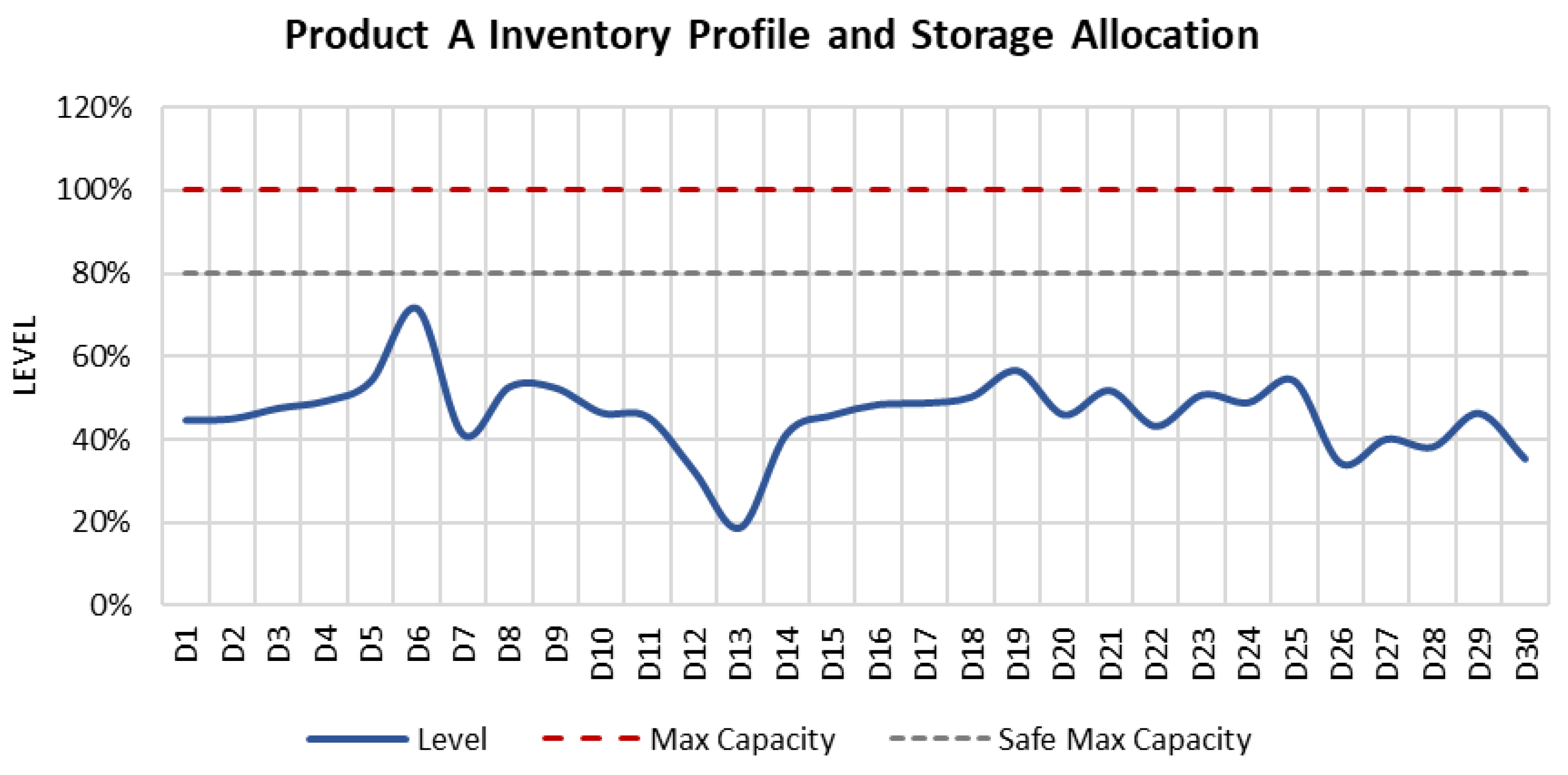
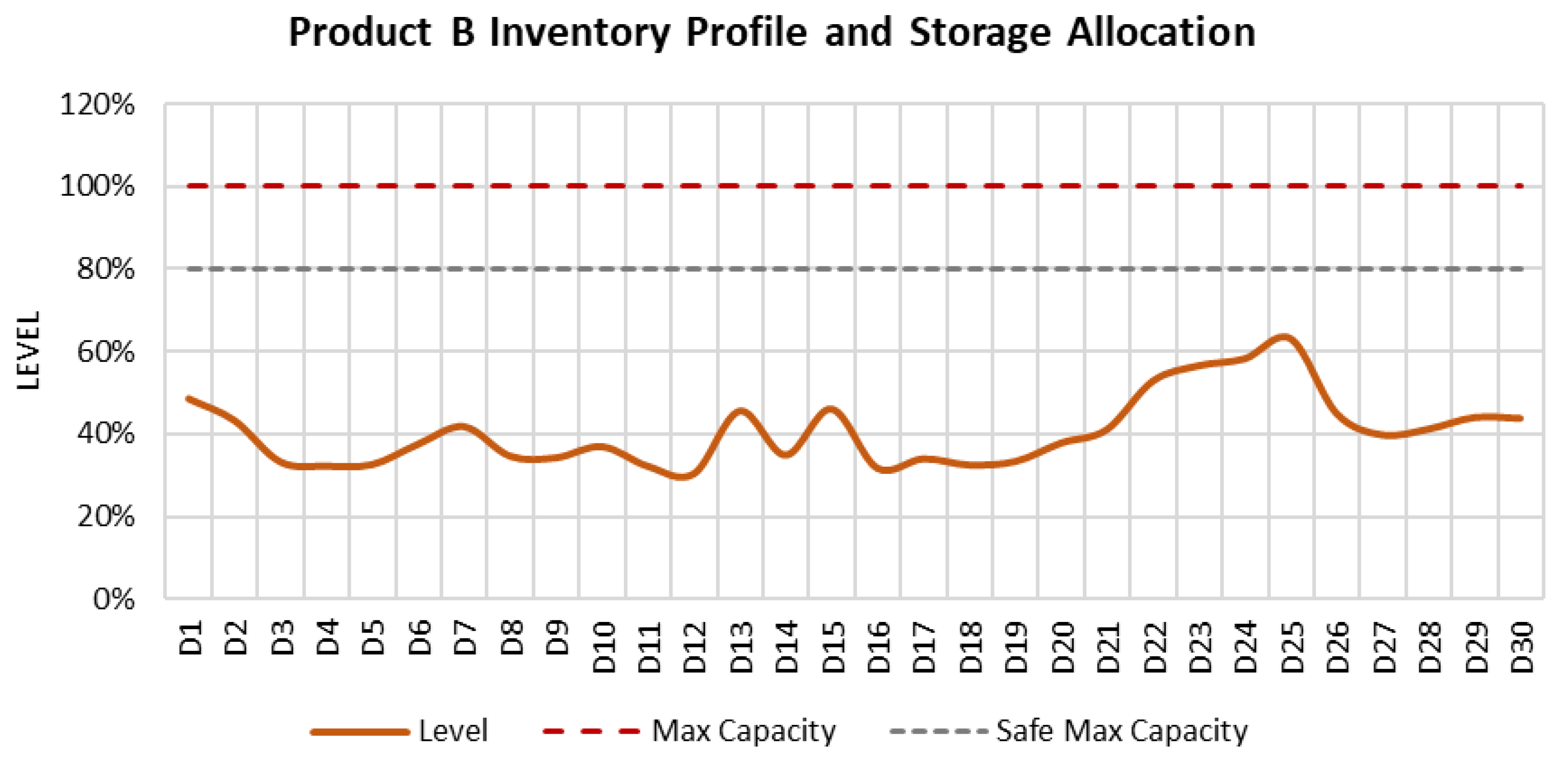
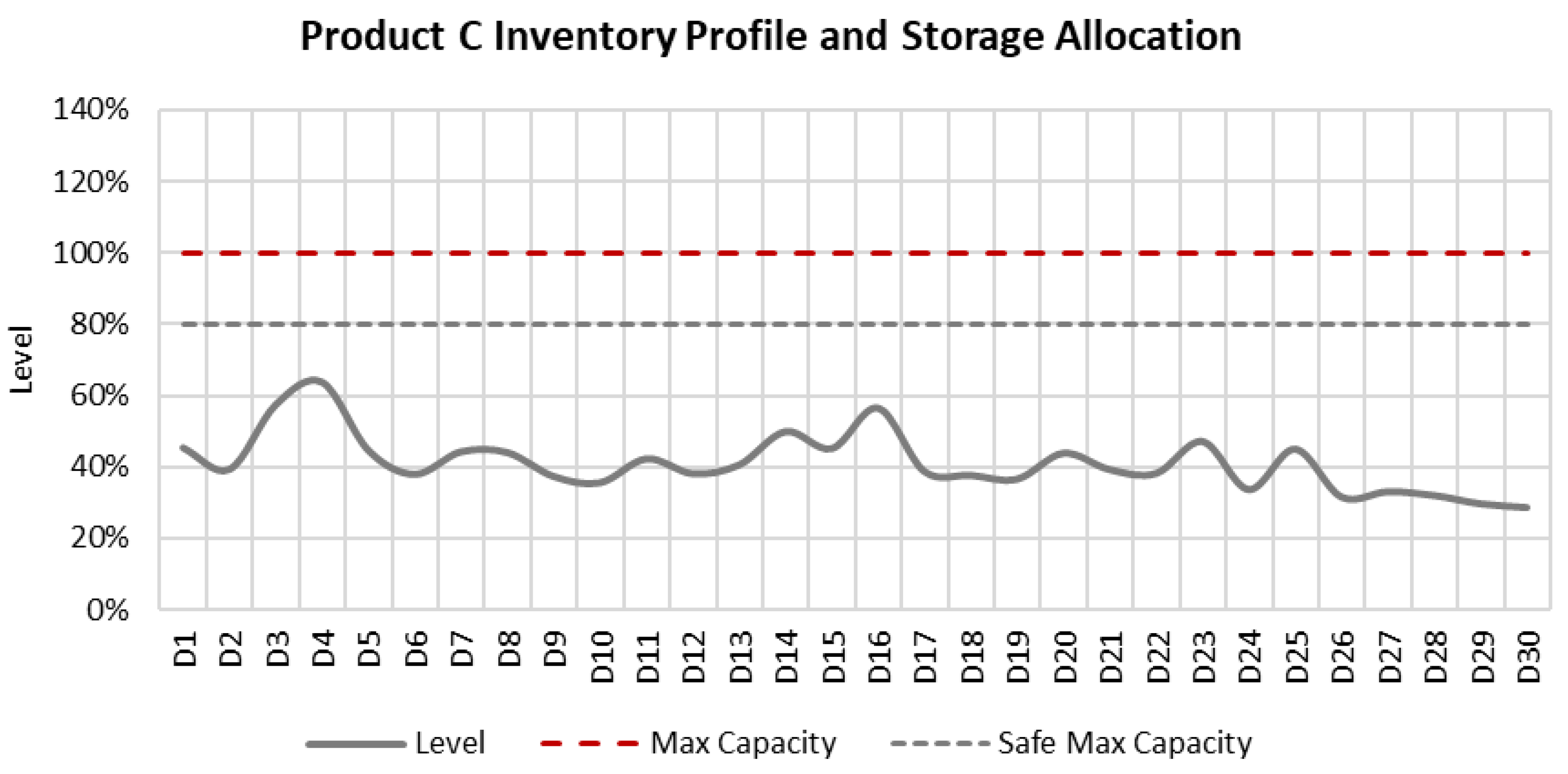
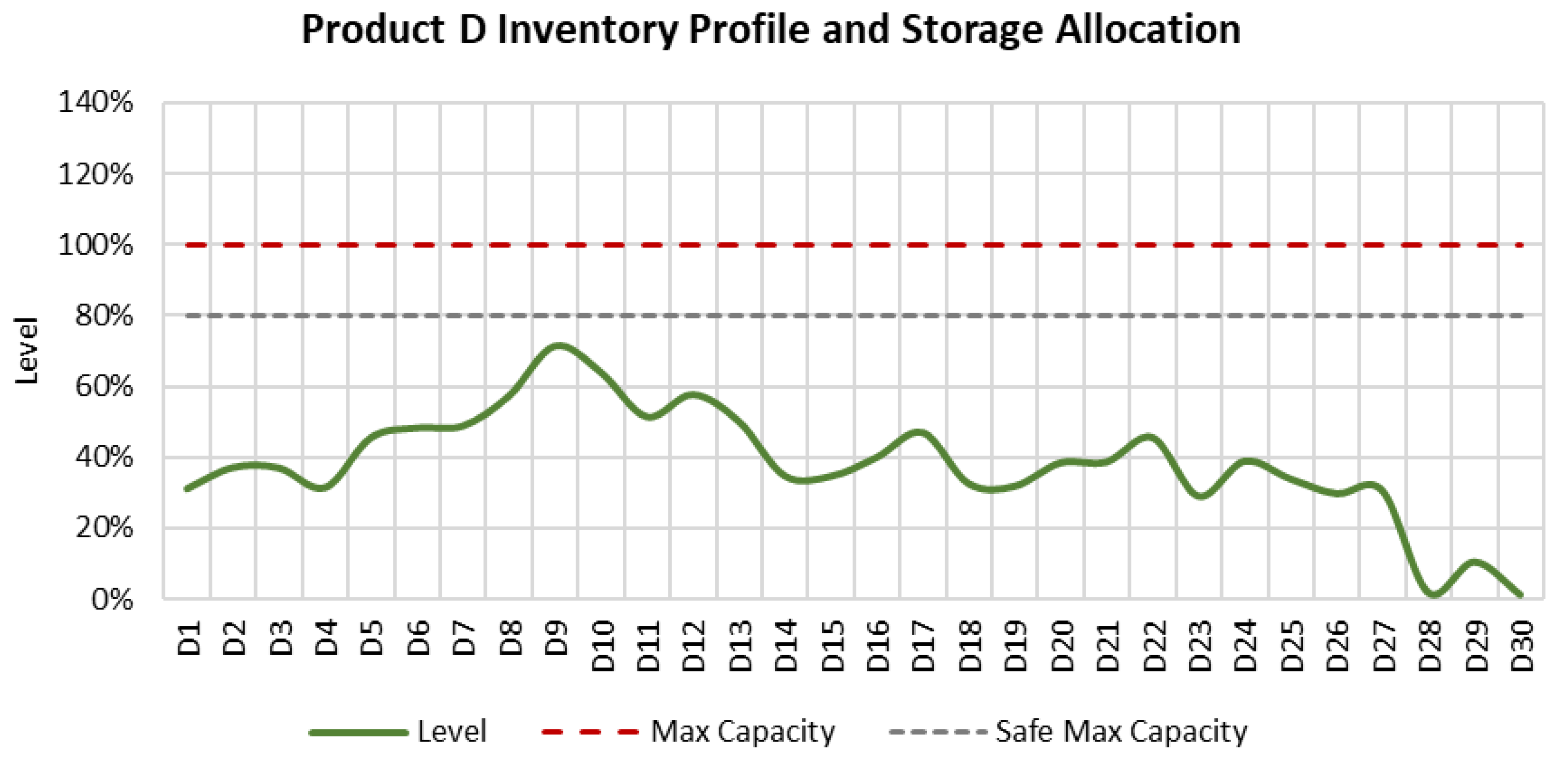
Figure 8, Figure 9, Figure 10 and Figure 11 illustrate the inventory profiles that were obtained from the model’s solution. All physical inventory limits are respected, and the model maintains inventory levels below the soft maximum limit of 80% capacity. Additionally, the graphs show how the model was able to maintain the projected inventories without altering tanks’ service, which is one of the objectives to be optimized.

6.6.2. Product Loading

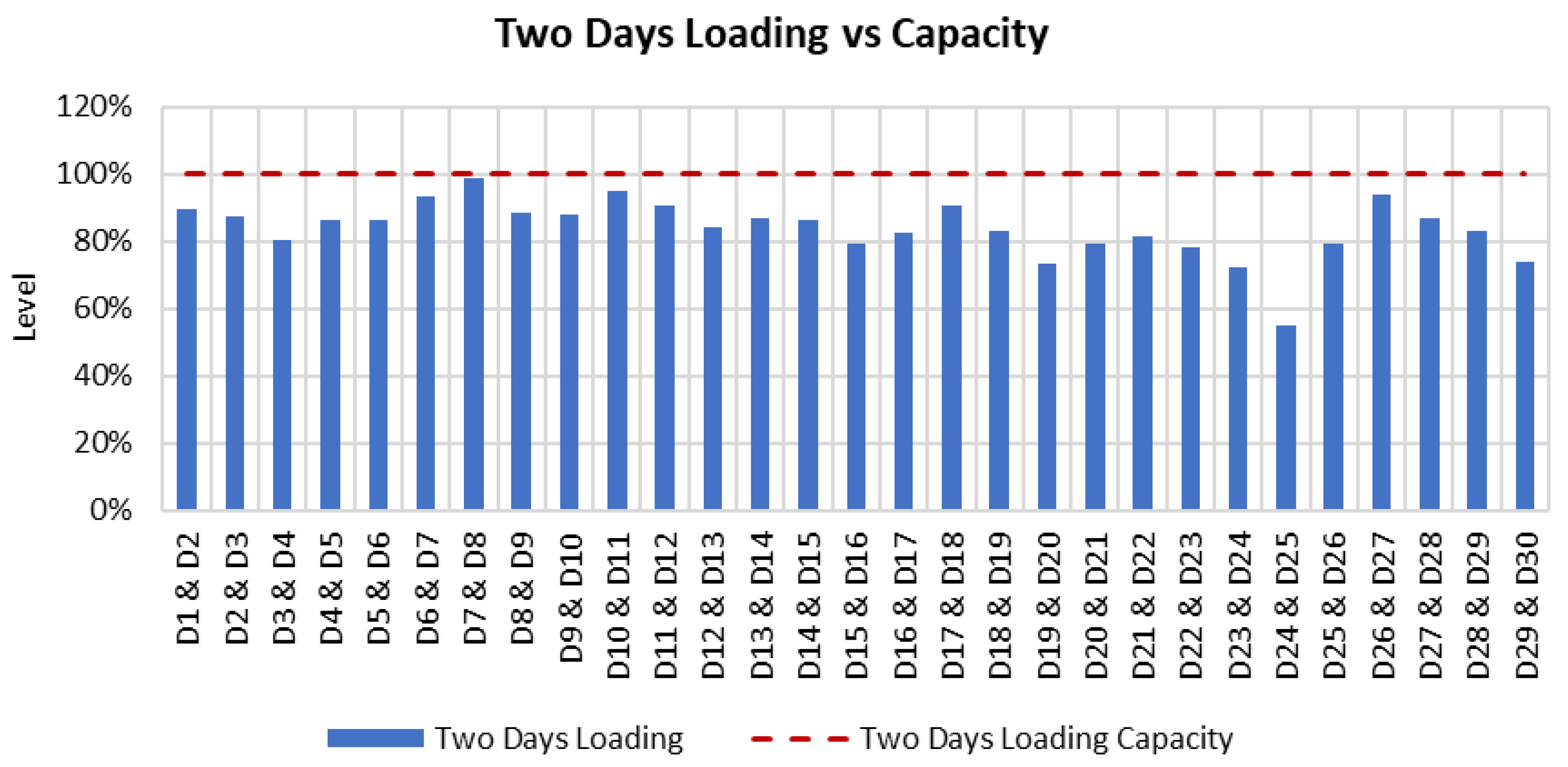
The solution maintained the level of loading quantities within the capacity of the terminal. Figure 12 illustrates the two consecutive days’ loading volumes against the two consecutive days’ capacity.

6.6.3. Crude Carriers’ Loading Day Distribution

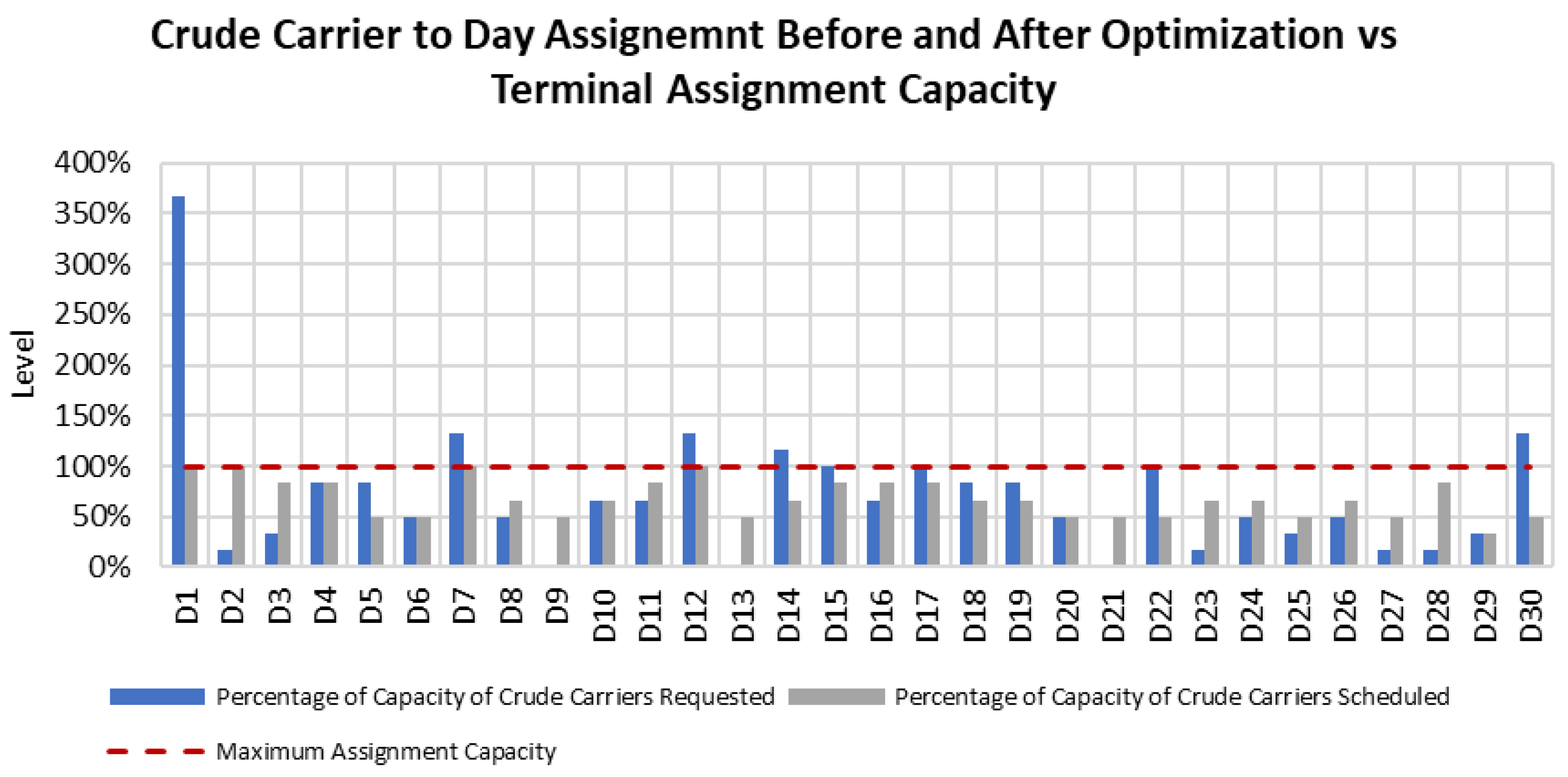
Figure 13 shows the crude carrier assignment before and after the optimization. Many customers prefer to load their cargoes on the first of the month, and the terminal capacity cannot accommodate all of them. In addition, it is noticed that for several days at the middle and end of the month, many carriers request to load their cargoes and exceed the terminal capacity. The solution distributes the crude carriers along the month to comply with the terminal assignment capacity. Load balancing was achieved by introducing the loading capacity constraint, where the problem started with an unfeasible solution with respect to the customer loading date, and the model changed the loading dates, with minimum deviation from the preferred loading date, to produce a feasible solution within the loading capacity limit.

6.6.4. Loading Day Deviation from Requested Day

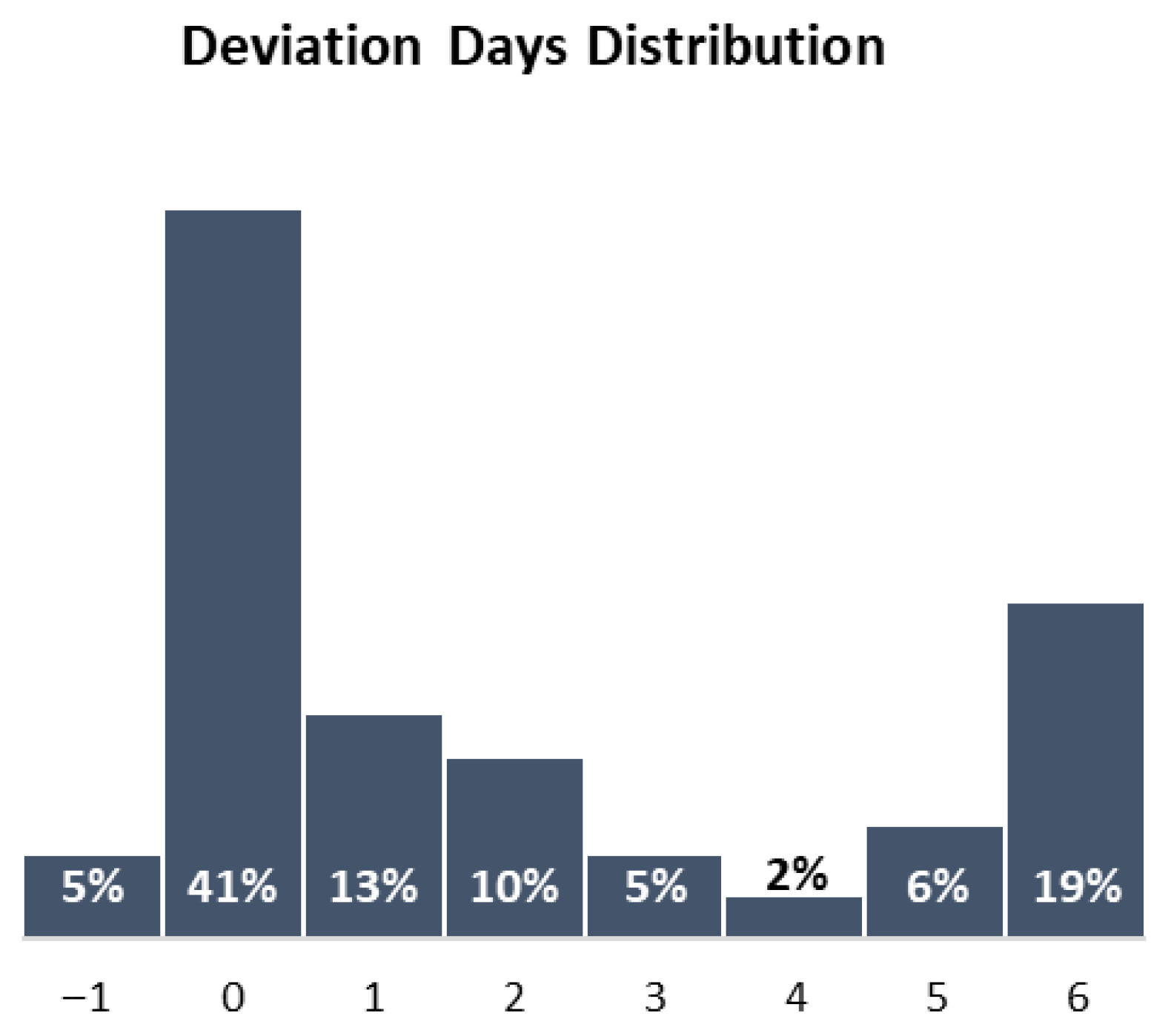
The primary objective of the model is to minimize the deviation between the actual and requested loading days. Analysis of the scheduling results shows that 53% of carriers are loaded within 2 days of their requested date, 15% within 3 to 4 days, and 32% within 5 to 6 days of deviation, as illustrated in Figure 14. These results highlight the model’s effectiveness in aligning actual loading schedules with customer preferences while identifying the proportion of carriers subject to longer deviations.

7. Conclusions and Future Research Direction

The COTS problem from the supplier perspective has not been investigated enough in the literature. The COTS is customer-centric, with dynamic inventory capacity management that integrates customers’ satisfaction with safe operating levels. The objective of this paper is to investigate the COTS for multiproduct dynamic storage capacity. In the literature, the majority of the papers are concerned with problems related to vessel routing and berth allocation in the field of marine supply. In this paper, a novel MIP formulation for crude oil export scheduling is developed that captures business requirements such as minimizing the maximum deviation from the customers’ requested loading date and maintaining a safe level of inventory for all products, with the ability to dynamically reallocate storage capacity for available products.

The problem is solved using three approaches: WS, HO, and WT. The WT method produced a better solution compared to the WS approach in alignment with the business-prioritized requirements. Adding its flexibility to fine-tune the weights for the objectives to adapt the dynamics of the problem makes it the best approach compared to the other two. However, utilizing the WT can be time-consuming, especially in obtaining the best available values for each objective and finding the minimum and maximum values to scale the function.

Furthermore, since the problem is modeled as an MILP, its performance can be enhanced by repressing the time variables to be continuous instead of discrete variables. Additionally, finding an exact solution in a short time is a challenge with this type of model; hence, exploring a heuristic approach may reduce the time to find a near-optimal solution. Finally, integrating the whole crude oil supply from the production facilities to the customers can be researched to produce a holistic model that can produce production and export plans that minimize inventory-related costs and maintain high service levels.

Reinforcement learning has shown promise in addressing scheduling problems. As the volatility and complexity of actual port settings escalate [55], training utilizing more efficient learning methodologies will further augment operational efficiency.