Distributed Robust Algorithms with Dependent Sampling

Abstract

Robust algorithms have been widely used and intensively studied in the communities of engineering, statistics, and machine learning since such algorithms are less sensitive to outliers and effective in addressing the issue of non-Gaussian noise during the learning process. In this paper we study the learning performance of a distributed robust algorithm with mixing dependent samples, where big data are collected distributively and have a dependence structure. Learning rates are derived by means of an integral operator decomposition technique and probability inequalities in Hilbert spaces. The results show that with a suitable robustification parameter, the performance of the distributed robust algorithm is comparable with that of its non-distributed counterpart, even if the dependent feature restricts the availability and the effective amount of data.

1. Introduction

Regression analysis plays an important role in the framework of supervised learning, which aims at estimating the function relations between input data and output data. The ordinary least-squares (OLS) method is widely employed for regression learning in real applications. However, when the sampling data are contaminated by high levels of noise, OLS behaves poorly since it belongs to two-moment statistical methods and cannot capture the high-moment information contained in the data. To tackle this problem, new learning methods are increasingly developed that are robust to heavy-tailed data or other potential forms of contamination. Among them, various robust loss functions are proposed to replace the least squares loss function, which can overcome the limitation of OLS caused by the characteristic of second-order statistics (see [1,2,3,4,5,6,7,8,9]). In this paper we focus on the robust loss functions of the form

$$\begin{array}{c}\hfill V_h\left(z\right)=G\left(\frac{z^2}{h^2}\right)\end{array}$$

(1)

induced by a windowing function $G:\mathcal{R}\to {\mathcal{R}}_{+}$ and the robustification parameter $h.$ Here the windowing function G is required to satisfy the following two conditions:

• For any $s\ge 0,G^{\prime }\left(s\right)>0$ and $G\left(s\right)\ge G\left(0\right)$. In addition, $C_G:={sup}_{s>0}|G^{\prime }\left(s\right)|<\infty$.
• There exists some $p>0$ such that for some constant $c_p>0$,

  $$\begin{array}{c}\hfill |G^{\prime }\left(s\right)-G^{\prime }\left(0\right)|\le c_p{|s|}^p,s>0.\end{array}$$

  (2)

Some commonly used robust loss functions fall into this category and are listed below.

• Fair loss function: $V_h\left(z\right)=\frac{|z|}{h}-log\left(1+\frac{|z|}{h}\right),G\left(s\right)=\sqrt{s}=log(1+\sqrt{s}),p=\frac{1}{2}$, $c_p=\frac{1}{2}$;
• Cauchy loss function: $V_h\left(z\right)=log\left(1+\frac{z^2}{2h^2}\right),G\left(s\right)=log(1+\frac{s}{2}),p=1,c_p=\frac{1}{4}$;
• Correntropy loss function: $V_h\left(z\right)=1-exp\left\{-\frac{z^2}{2h^2}\right\},G\left(s\right)=1-exp\{-\frac{s}{2}\},p=1$, $c_p=\frac{1}{4}$;
• Huber loss function: $V_h\left(z\right)={\mathbb{I}}_{|z|\le h}\frac{z^2}{2h^2}+{\mathbb{I}}_{|z|>h}\left(\frac{|z|}{h}-\frac{1}{2}\right),G\left(s\right)={\mathbb{I}}_{|z|\le h}\frac{s}{2}+{\mathbb{I}}_{|z|>h}\left(s^{\frac{1}{2}}-\frac{1}{2}\right),$$p=0,c_p=\frac{1}{2}$.

We can easily check that the windowing function G has the redescending property [4]. That is, when $|s|\le h$, the loss is convex and behaves like the least-squares loss; when $|s|\ge h$ the loss function tends to be concave and rapidly decreases to be flat as $|s|$ goes far from zero. Therefore, with a suitable chosen robustification parameter h, robust loss can completely reject gross outliers while maintaining a prediction accuracy similar to that of least-squares losses. In this work, we are interested in the application of robust loss in regression problems, linked to the data generation model given as

$$\begin{array}{c}\hfill Y=f^{\ast }\left(X\right)+\epsilon ,\mathbb{E}[\epsilon |X=x]=0.\end{array}$$

(3)

Here X is the input variable that takes values in a separable metric space $\mathcal{X}$ and $Y\in \mathcal{Y}\subset \mathbb{R}$ stands for the output variable; $\epsilon$ is the noise of the model, having a conditional mean of zero with respect to given $X=x$. The main purpose of the regression problem is to estimate $f^{\ast }$ according to a set of sampling data $\mathbf{D}={\left\{(x_i,y_i)\right\}}_{i=1}^m\subset \mathcal{Z}:=\mathcal{X}\times \mathcal{Y}$ generated by model (3).

Distributed learning has received considerable attention for the rapid expansion of computing capacities in the era of big data. Due to privacy concerns and communication cost, this paper studies a distributed robust algorithm with one communication round, based on the divide-and-conquer principle (DC). DC starts by using a massive data set that is stored distributively in local machines or dividing the whole data set into multiple subsets that are distributed to local machines, then takes a base algorithm to analyze the local data set, and finally averages all local estimators by only one communication to the master machine. It is thus computationally efficient by enabling parallel computing in the local learning process and can preserve data security and privacy without mutual information communications. This scheme has been developed for many classical learning algorithms, including kernel ridge regression, bias correction, minimum error entropy, and spectral algorithms, see [10,11,12,13,14,15,16,17,18].

During the data collection or assignment, the sampling data is generated from some non-trivial stochastic process with memory. In particular, when big data are collected in a temporal order, they display a dependence feature between samples. Typical examples include Monte Carlo estimation in the Markov chain, covariance matrix estimation for Markov-dependent samples, and multiarm bandit problems [19,20,21,22]. In the literature the mixing process is frequently used to model a dependence structure between samples due to its ubiquitousness in stationary stochastic processes [23,24], which will be described in the next section.

With the development of modern science and technology, data collection becomes easier and thus more big data have been obtained and stored. Besides the property of large scale, such data usually have temporal dependence characteristics, such as in economy, finance, biology, medicine, industry, agriculture, transportation, and other fields. It is thus worthy to investigate the learning ability of distributed algorithms in the mixing sampling process. Robust learning is widely employed for regression learning when the sampling data are contaminated by high levels of noise. Therefore, we shall investigate the interplay between the level of robustness, degree of dependence, partition number, and generalization ability. Our works will demonstrate that in robust learning, the distributed method with dependent sampling can obtain statistical optimality while reducing computation cost substantially.

The aim of this paper is to study the learning performance of distributed robust algorithms for mixing sequences of sampling data. Our theoretical results will be the capacity-dependent error bounds obtained by using a recently developed integral operator technique and probability inequalities in Hilbert spaces for mixing sequences. We prove that such a distributed learning scheme can obtain optimal learning rates in the regression setting if the robustification parameter is suitably chosen.

2. Main Results

In this section, we state our main results and discuss their relations to the existing works. For this purpose, we first introduce some notations and concepts.

2.1. Preliminaries and Problem Setup

Given the sequence of random variables ${\left\{x_i\right\}}_{i=1}^{\infty }$, let ${\mathcal{M}}_j^t:=\sigma (x_i:j\le i\le t),t\in \mathbf{N}$ be the sigma-algebra generated by the random variables $x_j,\cdots ,x_t$. The strong mixing condition and uniform mixing condition are defined as follows.

Definition 1.

For two σ-fields $\mathcal{E}$ and $\mathcal{F}$, define the α-coefficient as

$$\begin{array}{c}\hfill \alpha (\mathcal{E},\mathcal{F})=\underset{A\in \mathcal{E},B\in \mathcal{F}}{sup}|P(A\bigcap B)-P\left(A\right)P\left(B\right)|\end{array}$$

and ϕ-coefficient as

$$\begin{array}{c}\hfill \varphi (\mathcal{E},\mathcal{F})=\underset{A\in \mathcal{E},B\in \mathcal{F}}{sup}|P(A|B)-P\left(A\right)P\left(B\right)|.\end{array}$$

A set of random sequences $\left\{x_i\right\},i\ge 1,$ is said to satisfy a strongly mixing condition (or α-mixing condition) if

$$\begin{array}{c}\hfill {\alpha }_i=\underset{k\ge 1}{sup}\alpha \left({\mathcal{M}}_1^k,{\mathcal{M}}_{k+i}^{\infty }\right)\to 0,\mathit{as}i\to \infty .\end{array}$$

(4)

It satisfies a uniformly mixing condition (or ϕ-mixing condition) if

$$\begin{array}{c}\hfill {\varphi }_i=\underset{k\ge 1}{sup}\varphi \left({\mathcal{M}}_1^k,{\mathcal{M}}_{k+i}^{\infty }\right)\to 0,\mathit{as}i\to \infty .\end{array}$$

(5)

Remark 1.

When the sampling data ${\left\{x_i\right\}}_{i\ge 1}$ are drawn independently, both mixing conditions hold with ${\alpha }_i={\varphi }_i=0.$ According to the definitions, the strongly mixing condition is weaker than the ϕ-mixing condition. Many random processes satisfy the strongly mixing condition, for example, the stationary Markov process, which is uniformly purely non-deterministic, the stationary Gaussian sequence with a continuous spectral density that is bounded away from 0, certain ARMA processes, and some aperiodic Harris recurrent Markov processes; see [25,26].

In this work, we study the robust learning algorithm under the framework of reproducing kernel Hilbert space (RKHS) ${\mathcal{H}}_K$ [27]. Let $K:\mathcal{X}\times \mathcal{X}\to$ be a Mercer kernel, that is, a continuous, symmetric, and positive semi-definite function. The RKHS ${\mathcal{H}}_K$ associated with K is defined to be the completion of the linear span of the set of functions $\{K_x:=K(x,·),x\in \mathcal{X}\}$ equipped with the inner product ${⟨·,·⟩}_K$ satisfying the reproducing property

$$\begin{array}{c}\hfill {⟨g,K_x⟩}_K=g\left(x\right),foranyx\in \mathcal{X},g\in {\mathcal{H}}_K.\end{array}$$

(6)

Denote $\kappa :={sup}_{x\in \mathcal{X}}\sqrt{k(x,x)}$ [10]. This property implies that ${\parallel g\parallel }_{\infty }\le \kappa {\parallel g\parallel }_K,\forall g\in {\mathcal{H}}_K.$ Kernel methods provide efficient non-parametric learning algorithms for dealing with nonlinear features and RKHSs are used here as hypothesis spaces in the design of robust algorithms. Define the empirical robust risk over $\mathbf{D}={\left\{(x_i,y_i)\right\}}_{i=1}^m\subset \mathcal{Z}$,

$$\begin{array}{c}\hfill {\mathcal{E}}_D\left(f\right)=\frac{h^2}{2m}\sum _{(x,y)\in D}G\left(\frac{{\left[(f\left(x\right)-y)\right]}^2}{h^2}\right).\end{array}$$

Definition 2.

Given a sample set $\mathbf{D}={\left\{(x_i,y_i)\right\}}_{i=1}^m\subset \mathcal{Z}$, the regularized robust algorithm with an RKHS ${\mathcal{H}}_K$ in supervised learning is defined by

$$\begin{array}{c}\hfill f_{\mathbf{D},\lambda }=arg\underset{f\in {\mathcal{H}}_K}{min}{\mathcal{E}}_{\mathbf{D}}\left(f\right)+\frac{\lambda }{2}{\parallel f\parallel }_K^2\end{array}$$

(7)

where λ is a regularization parameter and h is a robustification parameter.

Distributed learning considered in the paper is applied to two real situations: 1. Data are collected and stored distributively and cannot be shared with each other due to privacy or communication cost. The typical example is continuous monitoring data from hospitals. 2. The collections of data have the time-serial property and the partitioning of data is performed sequentially. The typical example is spot price data. In the following, we describe the implementation of distributed learning in the two situations.

Based on DC, the implementation of (7) with distributed learning is described as follows:

• Decompose the data sets $\mathbf{D}$ into k disjoint subsets ${\left\{{\mathbf{D}}_{\ell }\right\}}_{\ell =1}^k$ of equal size so that each subset ${\mathbf{D}}_{\ell }$ has the sample size $|{\mathbf{D}}_{\ell }|=\frac{m}{k}=n$.
• Assign ${\mathbf{D}}_{\ell }$ to the ℓ-th local machine and produce the local estimator $f_{{\mathbf{D}}_{\ell },\lambda }$ using the base algorithm (7) performing on ${\mathbf{D}}_{\ell }.$
• Obtain the final estimator ${\overline{f}}_{\mathbf{D},\lambda }$ by averaging the local estimators

  $$\begin{array}{c}\hfill {\overline{f}}_{\mathbf{D},\lambda }=\frac{1}{k}\sum _{\ell =1}^k{f}_{{\mathbf{D}}_{\ell },\lambda }\end{array}$$

  (8)

When a sample set $\mathbf{D}={\left\{(x_i,y_i)\right\}}_{i=1}^m\subset \mathcal{Z}$ is drawn independently according to the identical distribution, it has been proven that for a broad class of algorithms, distributed learning has the same learning rates as its non-distributed counterpart as long as the local machines do not have too little training data [10,11,12,13]. When data have dependent structures, distributed regularized least-squares methods were shown in [22] to perform as well as the standard least-squares methods via attaining optimal learning rates. Their theoretical analysis is based on the characteristics of the squared losses, which cannot apply to the robust loss directly since it is not necessarily convex. Therefore, the learning performance of distributed robust algorithms under the dependency condition on the sampling data is still unknown.

2.2. Learning Rates

Throughout this paper, we assume that $\rho$ is a Borel probability measure on $\mathcal{Z}=\mathcal{X}\times \mathcal{Y}.$ The joint measure $\rho$ can be decomposed into

$$\begin{array}{c}\hfill \rho (x,y)=\rho (y|x){\mathbb{P}}_{\mathcal{X}}\left(x\right),z=(x,y)\in \mathcal{Z}\end{array}$$

where $\rho (y|x)$ is the conditional distribution on $\mathcal{Y}$ for given $\mathcal{X}=x$ and ${\rho }_{\mathcal{X}}$ is the marginal distribution of $\rho$ on $\mathcal{X}$ that describes the input data set ${\mathbf{D}}_{\mathcal{X}}={\left\{x_i\right\}}_{i=1}^m$. We assume the sample sequence ${\{z_i=(x_i,y_i)\}}_i$ comes from a strictly stationary process, and the dependence will be measured by the strongly mixing condition and uniformly mixing condition.

The goal of this paper is to estimate the learning error between ${\overline{f}}_{\mathbf{D},\lambda }$ and the target function $f^{\ast }$ in the $L_{{\mathbb{P}}_{\mathcal{X}}}^2$-space, that is $\parallel {\overline{f}}_{\mathbf{D},\lambda }-f^{\ast }{\parallel }_{L_{{\mathbb{P}}_{\mathcal{X}}}^2}^2$,

$$\begin{array}{c}\hfill L_{{\mathbb{P}}_{\mathcal{X}}}^2:=\left\{f:\mathcal{X}\to {\mathcal{R},\parallel f\parallel }_{L_{{\mathbb{P}}_{\mathcal{X}}}^2}={\int }_{\mathcal{X}}{|f\left(x\right)|}^{2}d{\mathbb{P}}_{\mathcal{X}}\left(x\right)<\infty \right\}.\end{array}$$

We now provide some necessary assumptions with respect to an integral operator $L_K:L_{{\mathbb{P}}_{\mathcal{X}}}^2⟶L_{{\mathbb{P}}_{\mathcal{X}}}^2$ associated with the kernel K by

$$\begin{array}{c}\hfill L_K\left(f\right):={\int }_{\mathcal{X}}f\left(x\right)K_{x}d{\mathbb{P}}_{\mathcal{X}},\forall f\in L_{{\mathbb{P}}_{\mathcal{X}}}^2.\end{array}$$

By the reproducing property of ${\mathcal{H}}_K,$ for any $f\in {\mathcal{H}}_K,$ it can be expressed as

$$\begin{array}{c}\hfill L_K\left(f\right)={\int }_{\mathcal{X}}{⟨f,K_x⟩}_K{K}_{x}d{\mathbb{P}}_{\mathcal{X}}\left(x\right),\forall f\in L_{{\mathbb{P}}_{\mathcal{X}}}^2.\end{array}$$

(9)

Since K is continuous, symmetric, and positive semi-definite, $L_K$ is a compact positive operator of trace class and $L_K+\lambda I$ is invertible for all $\lambda >0$.

Our first assumption is related to the complexity of the RKHS ${\mathcal{H}}_K,$ which can be measured by the concept effective dimension [10], that is, the trace of the operator ${(L_K+\lambda I)}^{-1}{L}_K$ defined as

$$\begin{array}{c}\hfill \mathcal{N}\left(\lambda \right)=Tr\left({(L_K+\lambda I)}^{-1}{L}_K\right),\lambda >0.\end{array}$$

Assumption 1.

With a parameter $0<s\le 1,$ there exists a constant $C_0>0$ such that $\mathcal{N}\left(\lambda \right)\le C_0{\lambda }^{-s}.$

Let ${\left\{{\mu }_i\right\}}_{i=1}^{\infty }$ be the eigenvalues of the operator $L_K$; then the eigenvalues of the operator ${(L_K+\lambda I)}^{-1}{L}_K$ are ${\left\{\frac{{\mu }_i}{{\mu }_i+\lambda }\right\}}_{i=1}^{\infty }$ and the trace $Tr\left({(L_K+\lambda I)}^{-1}{L}_K\right)$ is equal to ${\sum }_{i=1}^{\infty }\frac{{\mu }_i}{{\mu }_i+\lambda }.$ By the compactness of $\mathcal{X}$, we know that $Tr\left(L_K\right)<\infty .$ Hence, the above assumption is always satisfied with $s=1$ by taking the constant $C_0=Tr\left(L_K\right).$ When ${\mathcal{H}}_K$ is a finite rank space, for example, the linear space, the parameter s tends to 0. Furthermore, we assume that ${\left\{{\mu }_i\right\}}_{i=1}^{\infty }$ decays as ${\mu }_i=O\left(i^{-\frac{1}{b}}\right)$ for some $0<b<1$; then it is easy to check that $\mathcal{N}\left(\lambda \right)=O\left({\lambda }^{-b}\right).$ In fact, the effective dimension $\mathcal{N}\left(\lambda \right)$ is a common tool in leaning theory and spectral algorithms. It reflects the structure of the hypothesis space ${\mathcal{H}}_K$ and establishes a connection between integral operators and spectral methods. For more details, see [21].

The second assumption is stated in terms of the regularity of the target function $f^{\ast }.$

Assumption 2.

For some $r>0$ and $h_{\rho }\in L_{{\mathbb{P}}_{\mathcal{X}}}^2,$$f^{\ast }=L_K^r\left(h_{\rho }\right).$

Here $L_K^r$ denotes the r-th power of $L_K$, and it is well defined since $L_K$ is compact and positive. By the definition of ${\mathcal{H}}_K,$ we know that for any $f\in L_{{\mathbb{P}}_{\mathcal{X}}}^2$, ${\parallel f\parallel }_{L_{{\mathbb{P}}_{\mathcal{X}}}^2}={\parallel L_K^{\frac{1}{2}}f\parallel }_K.$ Then if $r\ge \frac{1}{2},$ it implies that $f^{\ast }$ lies in ${\mathcal{H}}_K.$ This assumption is called the Holder source condition [28] in inverse problems and characterizes the smoothness of the target function $f^{\ast }.$

In the sequel, let ${\parallel ·\parallel }_{\rho }:={\parallel ·\parallel }_{L_{{\mathbb{P}}_{\mathcal{X}}}^2}$ for simplicity and $|y|\le M$ almost surely for some constant $M>0.$ Without loss of generality, let $G^{\prime }\left(0\right)=1$ and $\kappa :={sup}_{x\in \mathcal{X}}\sqrt{k(x,x)}=1$. Our main results can be stated as follows. Here we assume that each sub-data set has the same size $|{\mathbf{D}}_{\ell }|=\frac{m}{k}=n$ for $1\le \ell \le k.$

Theorem 1.

Define ${\overline{f}}_{\mathbf{D},\lambda }$ by (8). Under Assumptions 1 and 2 with $0<s<1$ and $\frac{1}{2}<r\le 1,$ if the sample data $\mathbf{D}={\left\{(x_i,y_i)\right\}}_{i=1}^m$ satisfies the α-mixing condition, let $\lambda =m^{-\frac{1}{2r+s}},\delta >0$,

$$\begin{array}{cc}\hfill & \mathbb{E}[\parallel {\overline{f}}_{\mathbf{D},\lambda }-f^{\ast }{\parallel }_{\rho }]\hfill \\ \hfill & \le C_{1}k{m}^{-\frac{2r+s-1}{2r+s}}{\left(1+\sum _{\ell =1}^n{\alpha }_{\ell }\right)}^{\frac{1}{2}}\left(m^{\frac{s}{4r+2s}}+m^{\frac{2s+\delta }{(2r+s)(2\delta +4)}}{\left(\sum _{\ell =1}^n{\alpha }_{\ell }^{\frac{\delta }{2+\delta }}\right)}^{\frac{1}{2}}+m^{\frac{p+\frac{1}{2}}{2r+s}}{h}^{-2p}\right)\hfill \\ \hfill & +C_1\left(m^{-\frac{r}{2r+s}}+m^{\frac{2s+\delta }{(2r+s)(2\delta +4)}-\frac{1}{2}}{\left(\sum _{\ell =1}^m{\alpha }_{\ell }^{\frac{\delta }{2+\delta }}\right)}^{\frac{1}{2}}+h^{-2p}{m}^{\frac{p+1}{2r+s}}\right).\hfill \end{array}$$

(10)

where $C_1$ is a constant depending on the constants $C_0,r,s,M$ (appearing in the previous necessary assumptions), independent of $m,n,k,h$ (will be given in the proof).

A consequence of Theorem 1 is that the error bound for the distributed robust algorithm (8) depends on the partition number $k,$ robustification parameter h, and dependence coefficients ${\alpha }_{\ell }$. In particular, we have the following learning rates.

Corollary 1.

Under the same conditions as Theorem 1 with $2r+s>2$, if the α-mixing coefficients satisfy ${\alpha }_{\ell }=\mathcal{O}\left({\ell }^{-j}\right)$ with $j>1$ and

$$\begin{array}{c}\hfill k<m^{\frac{2r+s-2}{4r+2s}},\end{array}$$

(11)

then for any arbitarily small $ϵ>0,$

$$\begin{array}{cc}\hfill & \mathbb{E}[\parallel {\overline{f}}_{\mathbf{D},\lambda }-f^{\ast }{\parallel }_{\rho }]\le C_2\left(m^{-\frac{r+ϵ}{2r+s}}+h^{-2p}{m}^{\frac{p+1}{2r+s}}\right)\hfill \end{array}$$

(12)

where $C_2$ is a constant depending on the constants $C_0,r,s,M,j$ (appearing in the previous necessary assumptions), independent of $m,n,k,h$ (will be given in the proof).

Remark 2.

It was shown in [22] that the distributed least-squares method maintains the nearly optimal learning performance $\mathcal{O}\left(m^{-\frac{r+ϵ}{2r+s}}\right)$ for small enough $ϵ>0$ provided the number of local machines k is not so large and samples are drawn according to the α-mixing process. This corollary suggests that as the robustification parameter h increases, the learning rates can improve to the best order $\mathcal{O}\left(m^{-\frac{r+ϵ}{2r+s}}\right)$, coinciding with the results for the least-squares methods. However, further increasing of h beyond $m^{\frac{p+1+r}{2p(2r+s)}}$ may not help to improve the learning rate. This shows that h should keep a balance between the prediction accuracy and the degree of robustness during the training process.

For example, when ${\mathcal{H}}_K$ is a linear space and $f^{\ast }$ lies in ${\mathcal{H}}_K$, then s goes to 0 and $r=\frac{1}{2}.$ By Corollary 1, we deduce that the generalization error bound for the robust losses (including Huber loss) is on the order of $\mathcal{O}\left(m^{-\frac{1}{2}+{ϵ}^{\prime }}\right)$ (${ϵ}^{\prime }$ is arbitrarily small) by taking h large enough and ϵ small enough.

Next, Theorem 2 concerns the error bound for the distributed robust algorithm (8) under the $\varphi$-mixing process.

Theorem 2.

Define ${\overline{f}}_{\mathbf{D},\lambda }$ by (8). Under Assumptions 1,2 with $0<s<1$ and $\frac{1}{2}<r\le 1,$ if the sample data $\mathbf{D}={\left\{(x_i,y_i)\right\}}_{i=1}^m$ satisfies the ϕ-mixing condition, let $\lambda =m^{-\frac{1}{2r+s}},$

$$\begin{array}{cc}\hfill & \mathbb{E}[\parallel {\overline{f}}_{\mathbf{D},\lambda }-f^{\ast }{\parallel }_{\rho }]\hfill \\ \hfill & \le C_{3}k{m}^{-\frac{2r+s-1}{2r+s}}{\left(1+\sum _{\ell =1}^n{\varphi }_{\ell }\right)}^{\frac{1}{2}}\left(m^{\frac{s}{4r+2s}}+m^{\frac{s}{4r+2s}}{\left(\sum _{\ell =1}^n{\varphi }_{\ell }^{\frac{1}{2}}\right)}^{\frac{1}{2}}+m^{\frac{p+\frac{1}{2}}{2r+s}}{h}^{-2p}\right)\hfill \\ \hfill & +C_3\left(m^{-\frac{r}{2r+s}}+m^{-\frac{r}{2r+s}}{\left(\sum _{\ell =1}^m{\varphi }_{\ell }^{\frac{1}{2}}\right)}^{\frac{1}{2}}+h^{-2p}{m}^{\frac{p+1}{2r+s}}\right).\hfill \end{array}$$

(13)

where $C_3$ is a constant depending on the constants $C_0,r,s,M$ (appearing in the previous necessary assumptions), independent of $m,n,k,h$ (will be given in the proof).

Corollary 2.

Under the same conditions as Theorem 2 with $2r+s>2$, if the ϕ-mixing coefficients satisfy ${\varphi }_{\ell }=\mathcal{O}\left({\ell }^{-j}\right)$ with some $j>2$ and

$$\begin{array}{c}\hfill k<m^{\frac{2r+s-2}{4r+2s}},\end{array}$$

(14)

then

$$\begin{array}{cc}\hfill & \mathbb{E}[\parallel {\overline{f}}_{\mathbf{D},\lambda }-f^{\ast }{\parallel }_{\rho }]\le C_4\left(m^{-\frac{r}{2r+s}}+h^{-2p}{m}^{\frac{p+1}{2r+s}}\right)\hfill \end{array}$$

(15)

where $C_4$ is a constant depending on the constants $C_0,r,s,M,j$ (appearing in the previous necessary assumptions), independent of $m,n,k,h$ (will be given in the proof).

Remark 3.

Corollaries 1 and 2 tell us that distributed robust algorithms can achieve the same learning rate as that for independent samples if the mixing coefficients are summable, which was proved in [10]. Therefore, such algorithms have advantages in dealing with the large sample size and noise models.

3. Proofs

Now we are in a position of proving the consistency results stated in Section 2. First, we will give the error decomposition of $f_{\mathbf{D},\lambda }$ defined in algorithm (7).

3.1. Expression of $f_{\mathbf{D},\lambda }$

Define the empirical operator $L_{K,\mathbf{D}}:{\mathcal{H}}_K\to {\mathcal{H}}_K$ by

$$\begin{array}{c}\hfill L_{K,\mathbf{D}}:=\frac{1}{m}\sum _{x\in {\mathbf{D}}_{\mathcal{X}}}{⟨·,K_x⟩}_K{K}_x,\end{array}$$

So for any $f\in {\mathcal{H}}_K$, ${\displaystyle L_{K,\mathbf{D}}f=\frac{1}{m}\sum _{x\in {\mathbf{D}}_{\mathcal{X}}}f\left(x\right)K_x}$. Then we have the following representation for $f_{\mathbf{D},\lambda }$.

Lemma 1.

Define $f_{\mathbf{D},\lambda }$ by (7). Then it satisfies

$$\begin{array}{c}\hfill f_{\mathbf{D},\lambda }={(L_{K,\mathbf{D}}+\lambda I)}^{-1}{\hat{f}}_{\rho ,\mathbf{D}}+{(L_{K,\mathbf{D}}+\lambda I)}^{-1}{E}_{\mathbf{D},\lambda }\end{array}$$

(16)

where

$$\begin{array}{c}\hfill {\hat{f}}_{\rho ,\mathbf{D}}=\frac{1}{m}\sum _{(x,y)\in \mathbf{D}}y{K}_x\end{array}$$

and

$$\begin{array}{c}\hfill E_{\mathbf{D},\lambda }=\frac{1}{m}\sum _{(x,y)\in \mathbf{D}}\left[G^{\prime }\left(\frac{{(f_{\mathbf{D},\lambda }\left(x\right)-y)}^2}{h^2}\right)-G^{\prime }\left(0\right)\right](f_{\mathbf{D},\lambda }\left(x\right)-y)K_x.\end{array}$$

Proof. 

Since $f_{\mathbf{D},\lambda }$ is the minimizer of algorithm (7), we take the gradient of the regularized functional on ${\mathcal{H}}_K$ in (7) to give

$$\begin{array}{c}\hfill \frac{1}{m}\sum _{(x,y)\in \mathbf{D}}{G}^{\prime }\left(\frac{{(f_{\mathbf{D},\lambda }\left(x\right)-y)}^2}{h^2}\right)(f_{\mathbf{D},\lambda }\left(x\right)-y)K_x+\lambda f_{\mathbf{D},\lambda }=0,\end{array}$$

or equivalently (recall the assumption $G^{\prime }\left(0\right)=1$),

$$\begin{array}{c}\hfill \frac{1}{m}\sum _{(x,y)\in D}(f_{\mathbf{D},\lambda }\left(x\right)-y)K_x+\lambda f_{\mathbf{D},\lambda }-E_{\mathbf{D},\lambda }=0,\end{array}$$

which is $(L_{K,\mathbf{D}}+\lambda I)f_{\mathbf{D},\lambda }-{\hat{f}}_{\rho ,\mathbf{D}}-E_{\mathbf{D},\lambda }=0$.

The proof is completed. □

The quantity $E_{\mathbf{D},\lambda }$ is referred to as the robust error, which is determined by the degree of robustness in the training process and can be estimated as follows. By the definition of $f_{\mathbf{D},\lambda }$ in (7), we have that ${\mathcal{E}}_{\mathbf{D}}\left(f_{\mathbf{D},\lambda }\right)+\lambda {\parallel f_{\mathbf{D},\lambda }\parallel }_K^2\le {\mathcal{E}}_{\mathbf{D}}\left(0\right)$. Recall that $C_G={sup}_s|G^{\prime }\left(s\right)|$. With the fact that $G\left(0\right)<G\left(a\right)$ for all $a>0$ and considering Taylor expansion,

$$\begin{array}{cc}\hfill \lambda \parallel f_{\mathbf{D},\lambda }{\parallel }_K^2\le & {\mathcal{E}}_{\mathbf{D}}\left(0\right)-{\mathcal{E}}_{\mathbf{D}}\left(f_{\mathbf{D},\lambda }\right)\le \frac{h^2}{2m}\sum _{(x,y)\in \mathbf{D}}G\left(\frac{y^2}{h^2}\right)-\frac{h^{2}G\left(0\right)}{2}\hfill \\ \hfill \le & \frac{C_G}{2m}\sum _{(x,y)\in \mathbf{D}}{y}^2\le C_G{M}^2.\hfill \end{array}$$

It follows that

$$\begin{array}{c}\hfill \parallel f_{\mathbf{D},\lambda }{\parallel }_K\le \sqrt{C_G}{\lambda }^{-\frac{1}{2}}M.\end{array}$$

(17)

By (2), we see that

$$\begin{array}{cc}\hfill \parallel E_{\mathbf{D},\lambda }{\parallel }_K& \le c_p{h}^{-2p}\frac{1}{m}\sum _{(x,y)\in \mathbf{D}}{\left(\parallel f_{\mathbf{D},\lambda }{\parallel }_K+|y|\right)}^{2p+1}\hfill \\ \hfill & \le 2^{2p}{c}_p{h}^{-2p}\frac{1}{m}\sum _{(x,y)\in \mathbf{D}}\left(\parallel f_{\mathbf{D},\lambda }{\parallel }_K^{2p+1}+{|y|}^{2p+1}\right)\hfill \\ \hfill & \le 2^{2p}{c}_p{h}^{-2p}\left(\parallel f_{\mathbf{D},\lambda }{\parallel }_K^{2p+1}+M^{2p+1}\right).\hfill \end{array}$$

(18)

This in combination with the bounds (17) gives that

$$\begin{array}{c}\hfill \parallel E_{\mathbf{D},\lambda }{\parallel }_K\le c_{p,M}\left({\lambda }^{-(p+\frac{1}{2})}+1\right)h^{-2p}\end{array}$$

(19)

where $c_{p,M}=2^{2p}{c}_p(C_G^{p+\frac{1}{2}}+1)M^{2p+1}$.

3.2. Error Decomposition

To derive the explicit learning rate of the distributed algorithm (8), we define the regularization function $f_{\lambda }$ in ${\mathcal{H}}_K$,

$$\begin{array}{c}\hfill f_{\lambda }:=arg\underset{f\in {\mathcal{H}}_K}{min}{\mathcal{E}}_{\mathsf{ls}}\left(f\right)+\lambda {\parallel f\parallel }_K^2\end{array}$$

where ${\mathcal{E}}_{\mathsf{ls}}\left(f\right)={\int }_{\mathcal{Z}}{(f\left(x\right)-y)}^{2}d\rho$ is the expected risk associated with the least-squares loss. It was proved in [29] that

$$\begin{array}{c}\hfill f_{\lambda }={(L_K+\lambda I)}^{-1}{L}_K{f}^{\ast },\end{array}$$

(20)

so $f_{\lambda }-f^{\ast }=-\lambda {(L_K+\lambda I)}^{-1}{f}^{\ast }$. Under Assumption 2 with $r>\frac{1}{2}$,

$$\begin{array}{c}\hfill \parallel f_{\lambda }-f^{\ast }{\parallel }_{\rho }\le {\parallel h_{\rho }\parallel }_{\rho }{\lambda }^r,\end{array}$$

(21)

and

$$\parallel f_{\lambda }{\parallel }_K\le {\parallel h_{\rho }\parallel }_{\rho }{\lambda }^{r-\frac{1}{2}}.$$

(22)

Now we state two error decompositions for $f_{\mathbf{D},\lambda }-f_{\lambda }$. By (20), $-L_{K,\mathbf{D}}{f}_{\lambda }-\lambda f_{\lambda }=-L_{K,\mathbf{D}}{f}_{\lambda }+L_K{f}_{\lambda }-L_K{f}^{\ast }$, so

$$\begin{array}{c}-f_{\lambda }={(L_{K,\mathbf{D}}+\lambda I)}^{-1}[(L_K-L_{K,D})f_{\lambda }-L_K{f}^{\ast }],\end{array}$$

(23)

and we obtain the first decomposition

$$\begin{array}{cc}\hfill f_{\mathbf{D},\lambda }-f_{\lambda }=& {(L_{K,\mathbf{D}}+\lambda I)}^{-1}(L_K-L_{K,\mathbf{D}})f_{\lambda }+{(L_{K,\mathbf{D}}+\lambda I)}^{-1}\left({\hat{f}}_{\rho ,\mathbf{D}}-L_K{f}^{\ast }\right)\hfill \\ \hfill & +{(L_{K,\mathbf{D}}+\lambda I)}^{-1}{E}_{\mathbf{D},\lambda }.\hfill \end{array}$$

(24)

Recall that $\lambda f_{\mathbf{D},\lambda }=-L_{K,\mathbf{D}}{f}_{\mathbf{D},\lambda }+{\hat{f}}_{\rho ,\mathbf{D}}+E_{\mathbf{D},\lambda }$, so

$$\begin{array}{c}(L_K+\lambda I)f_{\mathbf{D},\lambda }=(L_K-L_{K,\mathbf{D}})(f_{\mathbf{D},\lambda }-f_{\lambda })+(L_K-L_{K,\mathbf{D}})f_{\lambda }+{\hat{f}}_{\rho ,\mathbf{D}}+E_{\mathbf{D},\lambda },\end{array}$$

and we obtain the second decomposition

$$\begin{array}{cc}\hfill & f_{\mathbf{D},\lambda }-f_{\lambda }=f_{\mathbf{D},\lambda }-{(L_K+\lambda I)}^{-1}{L}_K{f}^{\ast }={(L_K+\lambda I)}^{-1}[(L_K+\lambda I)f_{\mathbf{D},\lambda }-L_K{f}^{\ast }]\hfill \\ \hfill & ={(L_K+\lambda I)}^{-1}(L_K-L_{K,\mathbf{D}})(f_{\mathbf{D},\lambda }-f_{\lambda })+{(L_K+\lambda I)}^{-1}(L_K-L_{K,\mathbf{D}})f_{\lambda }\hfill \\ \hfill & +{(L_K+\lambda I)}^{-1}({\hat{f}}_{\rho ,\mathbf{D}}-L_K{f}^{\ast })+{(L_K+\lambda I)}^{-1}{E}_{\mathbf{D},\lambda }.\hfill \end{array}$$

(25)

3.3. Estimates in Distributed Learning

In order to deal with the mixing sequences, we use the following two lemmas, which can be found in [21]. For a random variable $\xi$ with values in a Hilbert space $\mathcal{H}$ and $1\le u\le \infty$, denote ${\parallel \xi \parallel }_u={(\mathbb{E}\parallel \xi \parallel }_{\mathcal{H}}^u{)}^{1/u}$ if $1\le u<\infty$ and ${\parallel \xi \parallel }_{\infty }=sup{\parallel \xi \parallel }_{\mathcal{H}}.$

Lemma 2.

Let ξ and η be random variables with values in separable Hilbert space $\mathcal{H}$ measurable σ-fields $\mathcal{E}$ and $\mathcal{F}$ with finite u-th and v-th moments, respectively. If $1<u,v,t<\infty$ with $u^{-1}+v^{-1}+t^{-1}=1,$ then

$$\begin{array}{c}\hfill |\mathbb{E}(\xi ,\eta )-(\mathbb{E}\xi ,\mathbb{E}\eta )|\le 15{\alpha }^{\frac{1}{t}}(\mathcal{E},\mathcal{F}){\parallel \xi \parallel }_u{\parallel \eta \parallel }_v.\end{array}$$

(26)

Lemma 3.

Let ξ and η be random variables with values in separable Hilbert space $\mathcal{H}$ measurable σ-fields $\mathcal{E}$ and $\mathcal{F}$ with finite p-th and q-th moments, respectively. If $1\le p,q<\infty$ with $p^{-1}+q^{-1}=1,$ then

$$\begin{array}{c}\hfill |\mathbb{E}(\xi ,\eta )-(\mathbb{E}\xi ,\mathbb{E}\eta )|\le 2{\varphi }^{\frac{1}{p}}(\mathcal{E},\mathcal{F}){\parallel \xi \parallel }_p{\parallel \eta \parallel }_q.\end{array}$$

(27)

Next, we define some notations used in this paper.

$$\begin{array}{cc}\hfill & \mathcal{A}(\mathbf{D},\lambda ):=\mathbb{E}[\parallel {(L_k+\lambda I)}^{-\frac{1}{2}}(L_K-L_{K,\mathbf{D}}){\parallel }^2],\hfill \\ \hfill & \mathcal{B}(\mathbf{D},\lambda ):=\mathbb{E}[\parallel {(L_k+\lambda I)}^{-1}(L_K+\lambda I)\parallel ],\hfill \\ \hfill & \mathcal{C}(\mathbf{D},\lambda ):=\mathbb{E}[\parallel {(L_k+\lambda I)}^{-\frac{1}{2}}(L_K{f}^{\ast }-{\hat{f}}_{\rho ,\mathbf{D}}){\parallel }_K^2],\hfill \\ \hfill & \mathcal{I}\left(\mathbf{D}\right):=\mathbb{E}[\parallel L_K-L_{K,\mathbf{D}}{\parallel }^2],\hfill \\ \hfill & \mathcal{J}\left(\mathbf{D}\right):=\mathbb{E}[\parallel L_K{f}^{\ast }-{\hat{f}}_{\rho ,\mathbf{D}}{\parallel }_K^2].\hfill \end{array}$$

Lemma 4.

If the sample sequence $\mathbf{D}={\left\{(x_i,y_i)\right\}}_{i=1}^m$ satisfies the α-mixing condition, then for any $\delta >0,$

$$\begin{array}{cc}\hfill & \mathcal{A}{(\mathbf{D},\lambda )}^{{\displaystyle \frac{1}{2}}}\le \sqrt{{\displaystyle \frac{\mathcal{N}\left(\lambda \right)}{m}}}+4{\displaystyle \frac{{\left(\mathcal{N}\left(\lambda \right)\right)}^{\frac{1}{2+\delta }}}{{\lambda }^{\frac{\delta }{2\delta +4}}}}\left(\sqrt{{\displaystyle \frac{1}{m}}\sum _{\ell }^m{\left({\alpha }_{\ell }\right)}^{{\displaystyle \frac{\delta }{2+\delta }}}}\right);\hfill \end{array}$$

(28)

$$\begin{array}{cc}\hfill & \mathcal{B}{(\mathbf{D},\lambda )}^{{\displaystyle \frac{1}{2}}}\le \sqrt{{\displaystyle \frac{2\mathcal{N}\left(\lambda \right)}{m\lambda }}}+6{\displaystyle \frac{{\left(\mathcal{N}\left(\lambda \right)\right)}^{\frac{1}{2+\delta }}}{{\lambda }^{\frac{\delta +1}{\delta +2}}}}\left(\sqrt{{\displaystyle \frac{1}{m}}\sum _{\ell }^m{\left({\alpha }_{\ell }\right)}^{{\displaystyle \frac{\delta }{2+\delta }}}}\right)+\sqrt{3};\hfill \end{array}$$

(29)

$$\begin{array}{cc}\hfill & \mathcal{C}{(\mathbf{D},\lambda )}^{{\displaystyle \frac{1}{2}}}\le M\sqrt{{\displaystyle \frac{\mathcal{N}\left(\lambda \right)}{m}}}+4M{\displaystyle \frac{{\left(\mathcal{N}\left(\lambda \right)\right)}^{\frac{1}{2+\delta }}}{{\lambda }^{\frac{\delta }{2\delta +4}}}}\left(\sqrt{{\displaystyle \frac{1}{m}}\sum _{\ell }^m{\left({\alpha }_{\ell }\right)}^{{\displaystyle \frac{\delta }{2+\delta }}}}\right);\hfill \end{array}$$

(30)

$$\begin{array}{cc}\hfill & \mathcal{I}{\left(\mathbf{D}\right)}^{{\displaystyle \frac{1}{2}}}\le {\displaystyle \frac{1}{\sqrt{m}}}{\left(1+30\sum _{\ell =1}^m{\alpha }_{\ell }\right)}^{{\displaystyle \frac{1}{2}}};\hfill \end{array}$$

(31)

$$\begin{array}{cc}\hfill & \mathcal{J}{\left(\mathbf{D}\right)}^{{\displaystyle \frac{1}{2}}}\le {\displaystyle \frac{M}{\sqrt{m}}}{\left(1+30\sum _{\ell =1}^m{\alpha }_{\ell }\right)}^{{\displaystyle \frac{1}{2}}}.\hfill \end{array}$$

(32)

If the sample sequence $\mathbf{D}={\left\{(x_i,y_i)\right\}}_{i=1}^m$ satisfies the ϕ-mixing condition, then

$$\begin{array}{cc}\hfill & \mathcal{A}{(\mathbf{D},\lambda )}^{{\displaystyle \frac{1}{2}}}\le \sqrt{{\displaystyle \frac{\mathcal{N}\left(\lambda \right)}{m}}}+\sqrt{{\displaystyle \frac{2\mathcal{N}\left(\lambda \right)}{m}}\sum _{\ell =1}^m{\varphi }_{\ell }^{{\displaystyle \frac{1}{2}}}};\hfill \end{array}$$

(33)

$$\begin{array}{cc}\hfill & \mathcal{B}{(\mathbf{D},\lambda )}^{{\displaystyle \frac{1}{2}}}\le \sqrt{{\displaystyle \frac{2\mathcal{N}\left(\lambda \right)}{m\lambda }}}+2\sqrt{{\displaystyle \frac{\mathcal{N}\left(\lambda \right)}{m\lambda }}\sum _{\ell =1}^m{\varphi }_{\ell }^{{\displaystyle \frac{1}{2}}}}+\sqrt{2};\hfill \end{array}$$

(34)

$$\begin{array}{cc}\hfill & \mathcal{C}{(\mathbf{D},\lambda )}^{{\displaystyle \frac{1}{2}}}\le M\sqrt{{\displaystyle \frac{\mathcal{N}\left(\lambda \right)}{m}}}+M\sqrt{{\displaystyle \frac{2\mathcal{N}\left(\lambda \right)}{m}}\sum _{\ell =1}^m{\varphi }_{\ell }^{{\displaystyle \frac{1}{2}}}};\hfill \end{array}$$

(35)

$$\begin{array}{cc}\hfill & \mathcal{I}{\left(\mathbf{D}\right)}^{{\displaystyle \frac{1}{2}}}\le {\displaystyle \frac{1}{\sqrt{m}}}{\left(1+4\sum _{\ell =1}^m{\varphi }_{\ell }\right)}^{{\displaystyle \frac{1}{2}}};\hfill \end{array}$$

(36)

$$\begin{array}{cc}\hfill & \mathcal{J}{\left(\mathbf{D}\right)}^{{\displaystyle \frac{1}{2}}}\le {\displaystyle \frac{M}{\sqrt{m}}}{\left(1+4\sum _{\ell =1}^m{\varphi }_{\ell }\right)}^{{\displaystyle \frac{1}{2}}}.\hfill \end{array}$$

(37)

Proof. 

When $\mathbf{D}={\left\{(x_i,y_i)\right\}}_{i=1}^m$ satisfies the $\alpha$-mixing, the estimates (28)–(32) can be found in [22]. We only consider the situation of $\varphi$-mixing. Define ${\eta }_1\left(x\right)={(L_K+\lambda I)}^{-\frac{1}{2}}{⟨·,K_x⟩}_K{K}_x,\forall x\in \mathcal{X}.$ It takes values on $\mathcal{H}\mathcal{S}\left({\mathcal{H}}_{\mathcal{K}}\right)$, which is the Hilbert space of Hilbert–Schmidt operators on ${\mathcal{H}}_{\mathcal{K}}$ with the inner product ${⟨A,B⟩}_{\mathcal{H}\mathcal{S}}=Tr\left(A^{T}B\right)$. The norm is given by ${\parallel A\parallel }_{\mathcal{H}\mathcal{S}}^2={\sum }_i{\parallel A{e}_i\parallel }_K^2$, where ${\left\{e_i\right\}}_i$ is an orthonormal basis on ${\mathcal{H}}_K$. $\mathcal{H}\mathcal{S}\left({\mathcal{H}}_{\mathcal{K}}\right)$ is a subspace of the space of bounded linear operators on ${\mathcal{H}}_{\mathcal{K}}$ with the norm relations

$$\begin{array}{c}\hfill \parallel A\parallel \le {\parallel A\parallel }_{\mathcal{H}\mathcal{S}},{\parallel AB\parallel }_{\mathcal{H}\mathcal{S}}\le \parallel A\parallel {\parallel B\parallel }_{\mathcal{H}\mathcal{S}}.\end{array}$$

It was proved in [10] that

$$\begin{array}{c}\hfill \mathbb{E}\left[\parallel {\eta }_1{\left(x\right)\parallel }_{\mathcal{H}\mathcal{S}}^2\right]\le \mathcal{N}\left(\lambda \right).\end{array}$$

Thus, for any $i,$ we have

$$\begin{array}{c}\hfill {\mathbb{E}}_{x_i}{⟨{\eta }_1\left(x_i\right),{\eta }_1\left(x_i\right)⟩}_{\mathcal{H}\mathcal{S}}=\mathbb{E}\left[\parallel {\eta }_1{\left(x\right)\parallel }_{\mathcal{H}\mathcal{S}}^2\right]\le \mathcal{N}\left(\lambda \right).\end{array}$$

(38)

For any $i<j$, by Lemma 3 with $p=q=2,$

$$\begin{array}{c}\hfill \left|\mathbb{E}{⟨{\eta }_1\left(x_i\right),{\eta }_1\left(x_j\right)⟩}_{\mathcal{H}\mathcal{S}}-{\parallel {(L_K+\lambda I)}^{-\frac{1}{2}}{L}_K\parallel }_{\mathcal{H}\mathcal{S}}^2\right|\le 2{\varphi }_{j-i}^{\frac{1}{2}}\mathbb{E}[\parallel {\eta }_1\left(x\right){\parallel }_{\mathcal{H}\mathcal{S}}^2]\le 2{\varphi }_{j-i}^{\frac{1}{2}}\mathcal{N}\left(\lambda \right).\end{array}$$

(39)

In the rest, denote ${\hat{\mathbb{E}}}_{\mathbf{D}}\left[{\eta }_1\right]={\sum }_{i=1}^m{(L_K+\lambda I)}^{-\frac{1}{2}}{⟨·,K_{x_i}⟩}_K{K}_{x_i}$. Then

$$\begin{array}{cc}\hfill & \mathbb{E}[\parallel {(L_k+\lambda I)}^{-\frac{1}{2}}(L_K-L_{K,D}){\parallel }^2]=\mathbb{E}\left[{⟨\mathbb{E}\left[{\eta }_1\right]-{\hat{\mathbb{E}}}_{\mathbf{D}}\left[{\eta }_1\right],\mathbb{E}\left[{\eta }_1\right]-{\hat{\mathbb{E}}}_{\mathbf{D}}\left[{\eta }_1\right]⟩}_{\mathcal{H}\mathcal{S}}\right]\hfill \\ \hfill & =\mathbb{E}\left[\parallel {\hat{\mathbb{E}}}_{\mathbf{D}}\left[{\eta }_1\right]{\parallel }_{\mathcal{H}\mathcal{S}}^2\right]-{\parallel {(L_K+\lambda I)}^{-\frac{1}{2}}{L}_K\parallel }_{\mathcal{H}\mathcal{S}}^2.\hfill \end{array}$$

(40)

Note that by (38) and (39),

$$\begin{array}{cc}\hfill & \mathbb{E}\left[\parallel {\hat{\mathbb{E}}}_{\mathbf{D}}\left[{\eta }_1\right]{\parallel }_{\mathcal{H}\mathcal{S}}^2\right]=\frac{1}{m^2}\sum _{i=1}^m\mathbb{E}[\parallel {\eta }_1\left(x_i\right){\parallel }_{\mathcal{H}\mathcal{S}}^2]+\frac{2}{m^2}\sum _{i<j}\mathbb{E}\left[⟨{\eta }_1\left(x_i\right),{\eta }_1\left(x_j\right)⟩\right]\hfill \\ & \le \frac{\mathcal{N}\left(\lambda \right)}{m}+{\parallel {(L_K+\lambda I)}^{-\frac{1}{2}}{L}_K\parallel }_{\mathcal{H}\mathcal{S}}^2+\frac{2\mathcal{N}\left(\lambda \right)}{m^2}\sum _{1\le i<j\le m}{\varphi }_{j-i}^{\frac{1}{2}}.\hfill \end{array}$$

Putting the estimate above into (40) yields

$$\begin{array}{c}\hfill \mathbb{E}[\parallel {(L_K+\lambda I)}^{-\frac{1}{2}}(L_K-L_{K,D}){\parallel }^2]\le \frac{\mathcal{N}\left(\lambda \right)}{m}++\frac{2\mathcal{N}\left(\lambda \right)}{m}\sum _{1\le \ell \le m}{\varphi }_{\ell }^{\frac{1}{2}}.\end{array}$$

(41)

Then the estimate (33) holds.

Now we turn to estimating (34).

$$\begin{array}{cc}\hfill & \mathbb{E}\left[{(L_{K,\mathbf{D}}+\lambda I)}^{-1}(L_K+\lambda I)\right]\hfill \\ \hfill & \le \frac{1}{\lambda }\mathbb{E}\left[\parallel {(L_k+\lambda I)}^{-\frac{1}{2}}(L_K-L_{K,\mathbf{D}}){\parallel }^2\right]+\frac{1}{\sqrt{\lambda }}{\left(\mathbb{E}\left[\parallel {(L_K+\lambda I)}^{-\frac{1}{2}}(L_K-L_{K,\mathbf{D}}){\parallel }^2\right]\right)}^{\frac{1}{2}}+1\hfill \\ \hfill & \le \frac{2}{\lambda }\mathbb{E}\left[\parallel {(L_k+\lambda I)}^{-\frac{1}{2}}(L_K-L_{K,\mathbf{D}}){\parallel }^2\right]+2\hfill \\ \hfill & \le \frac{2\mathcal{N}\left(\lambda \right)}{m\lambda }++\frac{4\mathcal{N}\left(\lambda \right)}{m\lambda }\sum _{1\le \ell \le m}{\varphi }_{\ell }^{\frac{1}{2}}+2.\hfill \end{array}$$

where the last inequality is obtained by (41). Formula (34) can be obtained directly.

We proceed to estimating (35). Define the random variable ${\eta }_3\left(z\right)={(L_K+\lambda )}^{-\frac{1}{2}}y{K}_x,z=(x,y)\in \mathcal{Z}.$ It takes values on ${\mathcal{H}}_K$, and

$$\begin{array}{c}\hfill \mathbb{E}\left[{\eta }_3\left(z\right)\right]={(L_K+\lambda I)}^{-\frac{1}{2}}{L}_K{f}^{\ast }\end{array}$$

Denote the empirical form of $\mathbb{E}\left[{\eta }_3\right]$ as ${\hat{\mathbb{E}}}_{\mathbf{D}}\left[{\eta }_3\right]={\sum }_{i=1}^m{(L_K+\lambda I)}^{-\frac{1}{2}}{\hat{f}}_{\rho ,\mathbf{D}}$. It is easy to check that $\parallel {\eta }_s{\left(z\right)\parallel }_K\le \frac{M}{\sqrt{\lambda }}$ and $\mathbb{E}[\parallel {\eta }_3\left(z\right){\parallel }_K^2\le M^2\mathcal{N}\left(\lambda \right)$. For any $i<j$, by Lemma 3 with $p=q=2,$

$$\begin{array}{c}\hfill \left|\mathbb{E}{⟨{\eta }_3\left(x_i\right),{\eta }_3\left(x_j\right)⟩}_K-{\parallel {(L_K+\lambda I)}^{-\frac{1}{2}}{L}_K{f}^{\ast }\parallel }_{\mathcal{H}\mathcal{S}}^2\right|\le 2{\varphi }_{j-i}^{\frac{1}{2}}\mathbb{E}[\parallel {\eta }_3\left(x\right){\parallel }_K^2]\le 2M^2{\varphi }_{j-i}^{\frac{1}{2}}\mathcal{N}\left(\lambda \right).\end{array}$$

(42)

Following similar procedures in estimating (33) again, we can get (35).

We are in the position of estimating (36). Define ${\eta }_2\left(x\right)={⟨·,K_x⟩}_K{K}_x$. Then for any $i,$ we have

$$\begin{array}{c}\hfill {\mathbb{E}}_{x_i}{⟨{\eta }_2\left(x_i\right),{\eta }_2\left(x_i\right)⟩}_{\mathcal{H}\mathcal{S}}=\mathbb{E}\left[\parallel {\eta }_2{\left(x\right)\parallel }_{\mathcal{H}\mathcal{S}}^2\right]\le 1\end{array}$$

(43)

due to $\kappa =1.$

For any $i<j$, by Lemma 3 with $p=1,q=\infty ,$

$$\begin{array}{c}\hfill \left|\mathbb{E}{⟨{\eta }_2\left(x_i\right),{\eta }_2\left(x_j\right)⟩}_{\mathcal{H}\mathcal{S}}-{\parallel L_K\parallel }_{\mathcal{H}\mathcal{S}}^2\right|\le 2{\varphi }_{j-i}\underset{x}{sup}[\parallel {\eta }_2\left(x\right){\parallel }_{\mathcal{H}\mathcal{S}}]\le 2{\varphi }_{j-i}.\end{array}$$

(44)

Following similar procedures in estimating (33), we can get estimate (36).

For estimating (37), we define ${\eta }_4\left(z\right)=y{K}_x,z=(x,y)\in \mathbf{D}.$ Then for any $i,$ we have

$$\begin{array}{c}\hfill {\mathbb{E}}_{z_i}{⟨{\eta }_4\left(z_i\right),{\eta }_4\left(z_i\right)⟩}_K=\mathbb{E}\left[y_i^{2}K(x_i,x_i)\right]\le M^2.\end{array}$$

(45)

For any $i<j$, by Lemma 3 with $p=1,q=\infty ,$

$$\begin{array}{c}\hfill \left|\mathbb{E}{⟨{\eta }_4\left(z_i\right),{\eta }_4\left(z_j\right)⟩}_K-{\parallel L_K{f}^{\ast }\parallel }_K^2\right|\le 2{\varphi }_{j-i}\underset{x}{sup}[\parallel {\eta }_4\left(z\right){\parallel }_K]\le 2M{\varphi }_{j-i}.\end{array}$$

(46)

Following similar procedures in estimating (36), we can get estimate (37).

The proof is finished. □

Proposition 1.

Under Assumptions 1,2 with $0<s<1$ and $\frac{1}{2}<r\le 1,$ we have

$$\begin{array}{cc}\hfill & \mathbb{E}[\parallel {\overline{f}}_{\mathbf{D},\lambda }-f^{\ast }{\parallel }_{\rho }]\hfill \\ & \le 2{\lambda }^{-1}\underset{\ell }{sup}\mathcal{A}{({\mathbf{D}}_l,\lambda )}^{\frac{1}{2}}\left(\left(\mathcal{I}{\left({\mathbf{D}}_{\ell }\right)}^{\frac{1}{2}}{\parallel h_{\rho }\parallel }_{\rho }+\mathcal{J}{\left({\mathbf{D}}_{\ell }\right)}^{\frac{1}{2}}+c_{p,M}\left({\lambda }^{-(p+\frac{1}{2})}+1\right)h^{-2p}\right)\right)\hfill \\ \hfill & +\mathcal{A}{(\mathbf{D},\lambda )}^{\frac{1}{2}}\parallel h_{\rho }{\parallel }_{\rho }+\mathcal{C}{(\mathbf{D},\lambda )}^{\frac{1}{2}}+c_{p,M}\left({\lambda }^{-(p+\frac{1}{2})}+1\right)h^{-2p}+{\parallel h_{\rho }\parallel }_{\rho }{\lambda }^r.\hfill \end{array}$$

(47)

Proof. 

We split $\parallel {\overline{f}}_{\mathbf{D},\lambda }-f^{\ast }{\parallel }_{\rho }$ into $\parallel {\overline{f}}_{\mathbf{D},\lambda }-f_{\lambda }{\parallel }_{\rho }$ and $\parallel f^{\ast }-f_{\lambda }{\parallel }_{\rho }.$ First, we use the decomposition (24) and get

$$\begin{array}{cc}\hfill & \mathbb{E}[\parallel f_{\mathbf{D},\lambda }-f_{\lambda }{\parallel }_K^2]\le 3\mathbb{E}[\parallel {(L_{K,\mathbf{D}}+\lambda I)}^{-1}(L_K-L_{K,\mathbf{D}})f_{\lambda }{\parallel }^2]\hfill \\ \hfill & +3\mathbb{E}[\parallel {(L_{K,\mathbf{D}}+\lambda I)}^{-1}\left({\hat{f}}_{\rho ,\mathbf{D}}-L_K{f}^{\ast }\right){\parallel }^2]+3\mathbb{E}[\parallel {(L_{K,\mathbf{D}}+\lambda I)}^{-1}{E}_{\mathbf{D},\lambda }{\parallel }^2]\hfill \\ \hfill & \le 3{\lambda }^{-2}\left(\mathcal{I}\left(\mathbf{D}\right)\parallel f_{\lambda }{\parallel }_K^2+\mathcal{J}\left(\mathbf{D}\right)+{\parallel E_{\mathbf{D},\lambda }\parallel }_K^2\right).\hfill \end{array}$$

(48)

By the definition of ${\mathcal{H}}_k$, we know that for any $f\in L_{{\rho }_{\mathcal{X}}}^2$, $\parallel L_K^{\frac{1}{2}}{f\parallel }_K={\parallel f\parallel }_{\rho }$; then

$$\begin{array}{c}\hfill \parallel {\overline{f}}_{\mathbf{D},\lambda }-f_{\lambda }{\parallel }_{\rho }=\parallel L_K^{\frac{1}{2}}({\overline{f}}_{\mathbf{D},\lambda }-f_{\lambda }){\parallel }_K\le {\parallel {(L_K+\lambda I)}^{\frac{1}{2}}({\overline{f}}_{\mathbf{D},\lambda }-f_{\lambda })\parallel }_K.\end{array}$$

Then by decomposition (25), we have

$$\begin{array}{cc}\hfill & \parallel {\overline{f}}_{\mathbf{D},\lambda }-f_{\lambda }{\parallel }_{\rho }\le \frac{1}{k}\sum _{l=1}^k{\parallel {(L_K+\lambda I)}^{-\frac{1}{2}}(L_K-L_{K,{\mathbf{D}}_l})(f_{{\mathbf{D}}_l,\lambda }-f_{\lambda })\parallel }_K\hfill \\ \hfill & +{∥\frac{1}{k}\sum _{l=1}^k{(L_K+\lambda I)}^{-\frac{1}{2}}(L_K-L_{K,{\mathbf{D}}_l})f_{\lambda }∥}_K\hfill \\ \hfill & +{∥\frac{1}{k}\sum _{l=1}^k{(L_K+\lambda I)}^{-\frac{1}{2}}\left({\hat{f}}_{\rho ,{\mathbf{D}}_l}-L_K{f}_{\rho }\right)∥}_K+{\lambda }^{-\frac{1}{2}}\frac{1}{k}\sum _{l=1}^k{∥E_{{\mathbf{D}}_l,\lambda }∥}_K\hfill \\ \hfill & =\frac{1}{k}\sum _{l=1}^k{\parallel {(L_K+\lambda I)}^{-\frac{1}{2}}(L_K-L_{K,{\mathbf{D}}_l})(f_{{\mathbf{D}}_l,\lambda }-f_{\lambda })\parallel }_K\hfill \\ \hfill & +{∥{(L_K+\lambda I)}^{-\frac{1}{2}}(L_K-L_{K,\mathbf{D}})f_{\lambda }∥}_K\hfill \\ \hfill & +{∥{(L_K+\lambda I)}^{-\frac{1}{2}}\left({\hat{f}}_{\rho ,\mathbf{D}}-L_K{f}_{\rho }\right)∥}_K+{\lambda }^{-\frac{1}{2}}\frac{1}{k}\sum _{l=1}^k{∥E_{{\mathbf{D}}_l,\lambda }∥}_K.\hfill \end{array}$$

Therefore, we have

$$\begin{array}{cc}\hfill \mathbb{E}[\parallel {\overline{f}}_{\mathbf{D},\lambda }-f_{\lambda }{\parallel }_{\rho }]& \le \mathbb{E}\left[\frac{1}{k}\sum _{l=1}^k{\parallel {(L_K+\lambda I)}^{-\frac{1}{2}}(L_K-L_{K,{\mathbf{D}}_l})(f_{{\mathbf{D}}_l,\lambda }-f_{\lambda })\parallel }_K\right]\hfill \\ \hfill & +\mathbb{E}\left[{∥{(L_K+\lambda I)}^{-\frac{1}{2}}(L_K-L_{K,\mathbf{D}})f_{\lambda }∥}_K\right]\hfill \\ \hfill & +\mathbb{E}\left[{∥{(L_K+\lambda I)}^{-\frac{1}{2}}\left({\hat{f}}_{\rho ,\mathbf{D}}-L_K{f}_{\rho }\right)∥}_K\right]+{\lambda }^{-\frac{1}{2}}\mathbb{E}\left[\frac{1}{k}\sum _{l=1}^k{∥E_{D_l,\lambda }∥}_K\right]\hfill \\ \hfill & \le \underset{\ell }{sup}\mathcal{A}{({\mathbf{D}}_l,\lambda )}^{\frac{1}{2}}{\left(\mathbb{E}[\parallel f_{{\mathbf{D}}_l,\lambda }-f_{\lambda }{\parallel }_K^2]\right)}^{\frac{1}{2}}+\mathcal{A}{(\mathbf{D},\lambda )}^{\frac{1}{2}}{\parallel f_{\lambda }\parallel }_K\hfill \\ \hfill & +\mathcal{C}{(\mathbf{D},\lambda )}^{\frac{1}{2}}+{\lambda }^{-\frac{1}{2}}\underset{\ell }{sup}{∥E_{{\mathbf{D}}_l,\lambda }∥}_K\hfill \end{array}$$

(49)

where the last inequality is obtained by the Cauchy inequality. Using (48) with $\mathbf{D}={\mathbf{D}}_{\ell }$ and putting it into the estimate above, we have

$$\begin{array}{cc}\hfill & \mathbb{E}[\parallel {\overline{f}}_{\mathbf{D},\lambda }-f^{\ast }{\parallel }_{\rho }]\le \mathbb{E}[\parallel {\overline{f}}_{\mathbf{D},\lambda }-f_{\lambda }{\parallel }_{\rho }]+\parallel f^{\ast }-f_{\lambda }{\parallel }_{\rho }]\hfill \\ & \le 2{\lambda }^{-1}\underset{\ell }{sup}\mathcal{A}{({\mathbf{D}}_l,\lambda )}^{\frac{1}{2}}{\left(\left(\mathcal{I}\left({\underset{\_}{\mathbf{D}}}_{\ell }\right)\parallel f_{\lambda }{\parallel }_K^2+\mathcal{J}\left({\mathbf{D}}_{\ell }\right)+{\parallel E_{{\mathbf{D}}_{\ell },\lambda }\parallel }_K^2\right)\right)}^{\frac{1}{2}}\hfill \\ \hfill & +\mathcal{A}{(\underset{\_}{\mathbf{D}},\lambda )}^{\frac{1}{2}}\parallel f_{\lambda }{\parallel }_K+\mathcal{C}{(\mathbf{D},\lambda )}^{\frac{1}{2}}+{\lambda }^{-\frac{1}{2}}\underset{\ell }{sup}{∥E_{{\mathbf{D}}_l,\lambda }∥}_K+{\parallel f^{\ast }-f_{\lambda }\parallel }_{\rho }.\hfill \end{array}$$

This together with (19) and (22) gives the desired conclusion. □

3.4. Proofs of the Main Results

Proof of Theorem 1. 

We apply Proposition 1 to prove our main results. With the choice of $\lambda =m^{-\frac{1}{2r+s}}$, by Assumption 1, we get

$$\begin{array}{c}\hfill {\lambda }^{-(p+\frac{1}{2})}=m^{\frac{p+\frac{1}{2}}{2r+s}},\end{array}$$

$$\begin{array}{cc}\hfill \mathcal{A}{(\mathbf{D},\lambda )}^{\frac{1}{2}}& \le \sqrt{C_0}{\lambda }^{-\frac{s}{2}}{m}^{-\frac{1}{2}}+4C_0^{\frac{1}{\delta +2}}{\lambda }^{-\frac{\delta +2s}{2\delta +4}}{m}^{-\frac{1}{2}}{\left(\sum _{\ell =1}^m{\alpha }_{\ell }^{\frac{\delta }{2+\delta }}\right)}^{\frac{1}{2}}\hfill \\ \hfill & =\sqrt{C_0}{m}^{-\frac{r}{2r+s}}+4C_0^{\frac{1}{\delta +2}}{m}^{\frac{2s+\delta }{(2r+s)(2\delta +4)}-\frac{1}{2}}{\left(\sum _{\ell =1}^m{\alpha }_{\ell }^{\frac{\delta }{2+\delta }}\right)}^{\frac{1}{2}}.\hfill \end{array}$$

Similarly, we obtain

$$\begin{array}{c}\hfill \mathcal{C}{(\mathbf{D},\lambda )}^{\frac{1}{2}}=M\left(\sqrt{C_0}{m}^{-\frac{r}{2r+s}}+6C_0^{\frac{1}{\delta +2}}{m}^{\frac{2s+\delta }{(2r+s)(2\delta +4)}-\frac{1}{2}}{\left(\sum _{\ell =1}^m{\alpha }_{\ell }^{\frac{\delta }{2+\delta }}\right)}^{\frac{1}{2}}\right).\end{array}$$

Next, by $|{\mathbf{D}}_{\ell }|=n=\frac{m}{k},$ we get

$$\begin{array}{cc}\hfill \mathcal{A}{({\mathbf{D}}_{\ell },\lambda )}^{\frac{1}{2}}& \le \sqrt{C_0}{\lambda }^{-\frac{s}{2}}{n}^{-\frac{1}{2}}+4C_0^{\frac{1}{\delta +2}}{\lambda }^{-\frac{\delta +2s}{2\delta +4}}{n}^{-\frac{1}{2}}{\left(\sum _{\ell =1}^n{\alpha }_{\ell }^{\frac{\delta }{2+\delta }}\right)}^{\frac{1}{2}}\hfill \\ \hfill & =k^{\frac{1}{2}}\left(\sqrt{C_0}{m}^{-\frac{r}{2r+s}}+4C_0^{\frac{1}{\delta +2}}{m}^{\frac{2s+\delta }{(2r+s)(2\delta +4)}-\frac{1}{2}}{\left(\sum _{\ell =1}^n{\alpha }_{\ell }^{\frac{\delta }{2+\delta }}\right)}^{\frac{1}{2}}\right).\hfill \end{array}$$

Similarly, we have

$$\begin{array}{cc}\hfill & \mathcal{I}{\left({\mathbf{D}}_{\ell }\right)}^{\frac{1}{2}}=k^{\frac{1}{2}}\frac{1}{\sqrt{m}}{\left(1+30\sum _{\ell =1}^n{\alpha }_{\ell }\right)}^{\frac{1}{2}};\hfill \\ \hfill & \mathcal{J}{\left({\mathbf{D}}_{\ell }\right)}^{\frac{1}{2}}=k^{\frac{1}{2}}\frac{M}{\sqrt{m}}{\left(1+30\sum _{\ell =1}^n{\alpha }_{\ell }\right)}^{\frac{1}{2}}.\hfill \end{array}$$

We find that

$$\begin{array}{cc}\hfill & {\lambda }^{-1}\underset{\ell }{sup}\mathcal{A}{({\mathbf{D}}_l,\lambda )}^{\frac{1}{2}}\left(\left(\mathcal{I}{\left({\mathbf{D}}_{\ell }\right)}^{\frac{1}{2}}{\parallel h_{\rho }\parallel }_{\rho }+\mathcal{J}{\left({\mathbf{D}}_{\ell }\right)}^{\frac{1}{2}}+c_{p,M}\left({\lambda }^{-(p+\frac{1}{2})}+1\right)h^{-2p}\right)\right)\hfill \\ \hfill & \le C_{1}k{m}^{-\frac{2r+s-1}{2r+s}}{\left(1+\sum _{\ell =1}^n{\alpha }_{\ell }\right)}^{\frac{1}{2}}\left(m^{\frac{s}{4r+2s}}+m^{\frac{2s+\delta }{(2r+s)(2\delta +4)}}{\left(\sum _{\ell =1}^n{\alpha }_{\ell }^{\frac{\delta }{2+\delta }}\right)}^{\frac{1}{2}}+m^{\frac{p+\frac{1}{2}}{2r+s}}{h}^{-2p}\right)\hfill \end{array}$$

with

$$C_1=30{(\sqrt{C_0}+6C_0^{\frac{1}{\delta +2}})}^2(\parallel h_{\rho }{\parallel }_{\rho }+1+2c_{p,M})$$

and

$$\begin{array}{cc}\hfill & \mathcal{A}{(\mathbf{D},\lambda )}^{\frac{1}{2}}\parallel h_{\rho }{\parallel }_{\rho }+\mathcal{C}{(\mathbf{D},\lambda )}^{\frac{1}{2}}+c_{p,M}\left({\lambda }^{-(p+\frac{1}{2})}+1\right)h^{-2p}+{\parallel h_{\rho }\parallel }_{\rho }{\lambda }^r\hfill \\ \hfill & \le C_1\left(m^{-\frac{r}{2r+s}}+m^{\frac{2s+\delta }{(2r+s)(2\delta +4)}-\frac{1}{2}}{\left(\sum _{\ell =1}^m{\alpha }_{\ell }^{\frac{\delta }{2+\delta }}\right)}^{\frac{1}{2}}+h^{-2p}{m}^{\frac{p+1}{2r+s}}\right).\hfill \end{array}$$

Putting the estimates into (47) yields the desired conclusion (10).

□

Proof of Corollary 1. 

We shall prove it by Theorem 1. Note that ${\alpha }_{\ell }=\mathcal{O}\left({\ell }^{-j}\right)$ with $j>1$; then there exists a constant $c_j$ such that ${\sum }_{\ell =1}^n{\alpha }_{\ell }^{\frac{1}{2}}\le c_j$. In addition, with arbitrarily small $\epsilon >0,$ we choose large enough $\delta =\left(\frac{(2+s)\epsilon }{2r+s}+4\right)/(j-1)$. By simple calculation,

$$\begin{array}{c}\hfill m^{\frac{2s+\delta }{(2r+s)(2\delta +4)}-\frac{1}{2}}{\left(\sum _{\ell =1}^n{\alpha }_{\ell }^{\frac{\delta }{2+\delta }}\right)}^{\frac{1}{2}}\le c_{j,\epsilon }{m}^{\frac{s+\epsilon }{4r+2s}}\end{array}$$

where $c_{j,\epsilon }$ is a constant depending only on $j,\epsilon ,r,s$, independent of m. Note that $m^{\frac{2s+\delta }{(2r+s)(2\delta +4)}-\frac{1}{2}}{\left({\sum }_{\ell =1}^m{\alpha }_{\ell }^{\frac{\delta }{2+\delta }}\right)}^{\frac{1}{2}}\le m^{\frac{2s+\delta }{(2r+s)(2\delta +4)}-\frac{1}{2}}{\left({\sum }_{\ell =1}^n{\alpha }_{\ell }^{\frac{\delta }{2+\delta }}\right)}^{\frac{1}{2}}\le c_{j,\epsilon }{m}^{\frac{s+2\epsilon }{4r+2s}}.$ Putting the estimates above into (10), we get

$$\begin{array}{cc}\hfill \mathbb{E}[\parallel {\overline{f}}_{\mathbf{D},\lambda }-f^{\ast }{\parallel }_{\rho }]& \le C_1(1+c_j)(1+c_{j,\epsilon })k\left(m^{-\frac{4r+s-2-2\epsilon }{4r+2s}}+h^{-2p}{m}^{\frac{p+\frac{1}{2}}{2r+s}}\right)\hfill \\ \hfill & +C_1(1+c_{j,\epsilon })\left(m^{-\frac{r+\epsilon }{2r+s}}+h^{-2p}{m}^{\frac{p+1}{2r+s}}\right).\hfill \end{array}$$

This together with (14) yields the desired conclusion by letting $C_2=C_1(1+c_j)(1+c_{j,\epsilon })$. □

Proof of Theorem 2. 

We also apply Proposition 1 to prove our Theorem 2. With the choice of $\lambda =m^{-\frac{1}{2r+s}}$, by Assumption 1, we get

$$\begin{array}{c}\hfill {\lambda }^{-(p+\frac{1}{2})}=m^{\frac{p+\frac{1}{2}}{2r+s}},\end{array}$$

$$\begin{array}{cc}\hfill \mathcal{A}{(\mathbf{D},\lambda )}^{\frac{1}{2}}& \le \sqrt{C_0}{\lambda }^{-\frac{s}{2}}{m}^{-\frac{1}{2}}+2C_0^{\frac{1}{\delta +2}}{\lambda }^{-\frac{\delta +2s}{2\delta +4}}{m}^{-\frac{1}{2}}{\left(\sum _{\ell =1}^m{\varphi }_{\ell }^{\frac{1}{2}}\right)}^{\frac{1}{2}}\hfill \\ \hfill & =\sqrt{C_0}{m}^{-\frac{r}{2r+s}}+2C_0^{\frac{1}{\delta +2}}{m}^{\frac{2s+\delta }{(2r+s)(2\delta +4)}-\frac{1}{2}}{\left(\sum _{\ell =1}^m{\varphi }_{\ell }^{\frac{1}{2}}\right)}^{\frac{1}{2}}.\hfill \end{array}$$

Similarly, we obtain

$$\begin{array}{c}\hfill \mathcal{C}{(\mathbf{D},\lambda )}^{\frac{1}{2}}=M\left(\sqrt{C_0}{m}^{-\frac{r}{2r+s}}+2C_0^{\frac{1}{\delta +2}}{m}^{\frac{2s+\delta }{(2r+s)(2\delta +4)}-\frac{1}{2}}{\left(\sum _{\ell =1}^m{\varphi }_{\ell }^{\frac{1}{2}}\right)}^{\frac{1}{2}}\right).\end{array}$$

Next, by $|{\mathbf{D}}_{\ell }|=n=\frac{m}{k},$ we get

$$\begin{array}{cc}\hfill \mathcal{A}{({\mathbf{D}}_{\ell },\lambda )}^{\frac{1}{2}}& \le \sqrt{C_0}{\lambda }^{-\frac{s}{2}}{n}^{-\frac{1}{2}}+2C_0^{\frac{1}{\delta +2}}{\lambda }^{-\frac{\delta +2s}{2\delta +4}}{n}^{-\frac{1}{2}}{\left(\sum _{\ell =1}^n{\varphi }_{\ell }^{\frac{1}{2}}\right)}^{\frac{1}{2}}\hfill \\ \hfill & =k^{\frac{1}{2}}\left(\sqrt{C_0}{m}^{-\frac{r}{2r+s}}+2C_0^{\frac{1}{\delta +2}}{m}^{\frac{2s+\delta }{(2r+s)(2\delta +4)}-\frac{1}{2}}{\left(\sum _{\ell =1}^n{\varphi }_{\ell }^{\frac{1}{2}}\right)}^{\frac{1}{2}}\right).\hfill \end{array}$$

Similarly, we have

$$\begin{array}{cc}\hfill & \mathcal{I}{\left({\mathbf{D}}_{\ell }\right)}^{\frac{1}{2}}=k^{\frac{1}{2}}\frac{1}{\sqrt{m}}{\left(1+4\sum _{\ell =1}^n{\varphi }_{\ell }^{\frac{1}{2}}\right)}^{\frac{1}{2}};\hfill \\ \hfill & \mathcal{J}{\left({\mathbf{D}}_{\ell }\right)}^{\frac{1}{2}}=k^{\frac{1}{2}}\frac{M}{\sqrt{m}}{\left(1+4\sum _{\ell =1}^n{\varphi }_{\ell }^{\frac{1}{2}}\right)}^{\frac{1}{2}}.\hfill \end{array}$$

Then,

$$\begin{array}{cc}\hfill & {\lambda }^{-1}\underset{\ell }{sup}\mathcal{A}{({\mathbf{D}}_l,\lambda )}^{\frac{1}{2}}\left(\left(\mathcal{I}{\left({\mathbf{D}}_{\ell }\right)}^{\frac{1}{2}}{\parallel h_{\rho }\parallel }_{\rho }+\mathcal{J}{\left({\mathbf{D}}_{\ell }\right)}^{\frac{1}{2}}+c_{p,M}\left({\lambda }^{-(p+\frac{1}{2})}+1\right)h^{-2p}\right)\right)\hfill \\ \hfill & \le C_{3}k{m}^{-\frac{2r+s-1}{2r+s}}{\left(1+\sum _{\ell =1}^n{\varphi }_{\ell }^{\frac{1}{2}}\right)}^{\frac{1}{2}}\left(m^{\frac{s}{4r+2s}}+m^{\frac{2s+\delta }{(2r+s)(2\delta +4)}}{\left(\sum _{\ell =1}^n{\varphi }_{\ell }^{\frac{1}{2}}\right)}^{\frac{1}{2}}+m^{\frac{p+\frac{1}{2}}{2r+s}}{h}^{-2p}\right)\hfill \end{array}$$

with

$$C_3=16{(\sqrt{C_0}+4C_0^{\frac{1}{\delta +2}})}^2(\parallel h_{\rho }{\parallel }_{\rho }+1+2c_{p,M})$$

and

$$\begin{array}{cc}\hfill & \mathcal{A}{(\mathbf{D},\lambda )}^{\frac{1}{2}}\parallel h_{\rho }{\parallel }_{\rho }+\mathcal{C}{(\mathbf{D},\lambda )}^{\frac{1}{2}}+c_{p,M}\left({\lambda }^{-(p+\frac{1}{2})}+1\right)h^{-2p}+{\parallel h_{\rho }\parallel }_{\rho }{\lambda }^r\hfill \\ \hfill & \le C_3\left(m^{-\frac{r}{2r+s}}+m^{\frac{2s+\delta }{(2r+s)(2\delta +4)}-\frac{1}{2}}{\left(\sum _{\ell =1}^m{\varphi }_{\ell }^{\frac{1}{2}}\right)}^{\frac{1}{2}}+h^{-2p}{m}^{\frac{p+1}{2r+s}}\right).\hfill \end{array}$$

Putting the estimates into (47) yields the desired conclusion (13).

□

Proof of Corollary 2. 

Note that ${\sum }_{\ell =1}^n{\varphi }_{\ell }^{\frac{1}{2}}<c$ for some $c>0$ due to ${\varphi }_{\ell }=\mathcal{O}\left({\ell }^{-j}\right)$ for $j>2$. Then following similar procedures to those in the proof of Corollary 1, we get

$$\begin{array}{cc}\hfill \mathbb{E}[\parallel {\overline{f}}_{\mathbf{D},\lambda }-f^{\ast }{\parallel }_{\rho }]& \le C_3{(1+c^{\frac{1}{2}})}^{2}k\left(m^{-\frac{4r+s-2}{4r+2s}}+h^{-2p}{m}^{\frac{p+\frac{1}{2}}{2r+s}}\right)\hfill \\ \hfill & +C_3(1+c^{\frac{1}{2}})\left(m^{-\frac{r}{2r+s}}+h^{-2p}{m}^{\frac{p+1}{2r+s}}\right).\hfill \end{array}$$

The restriction of k implies that $k{m}^{-\frac{4r+s-2}{4r+2s}}\le m^{-\frac{r}{2r+s}}$. Then the desired conclusion holds with $C_4=2C_3{(1+c^{\frac{1}{2}})}^2$.

□

4. Experimental Setup

We consider the non-parametric regression model

$$Y_t=f^{\ast }\left(X_t\right)+{\epsilon }_t,$$

where the regression function is chosen as

$$f^{\ast }\left(x\right)=sin\left(2\pi x\right)+0.3cos\left(4\pi x\right),$$

which is infinitely smooth and therefore satisfies the regularity assumptions of our theory for any $r>0$. The noise variables are generated independently as ${\epsilon }_t\sim \mathcal{N}(0,0.1^2)$ and are independent of the covariates $X_t$.

To instantiate the theoretical rates in a concrete manner, we fix the smoothness, capacity, and robustness indices as

$$r=1,s=\frac{1}{2}.$$

These choices correspond to a moderately smooth regression function, a kernel with effective dimension exponent $s=1/2$, and a light-tailed noise regime compatible with the Huber loss used in the algorithm.

Given $(r,s,p)$, the theoretically guided tuning parameters for distributed robust regression are set as

$${\lambda }_m=0.1m^{-1/(2r+s)}\mathrm{and}{h}_m=m^{{\gamma }_h},{\gamma }_h=\frac{p+1+r}{2p(2r+s)}=\frac{3}{5},$$

which agree with the convergence theory developed in this paper. All experiments employ the Gaussian kernel with bandwidth parameter $\gamma =1$ and the Huber loss.

For each sample size m, we draw a training sample ${\left\{(X_t,Y_t)\right\}}_{t=1}^m$ under the specified dependence structure and compute the distributed estimator using k machines, as described earlier. Each configuration is repeated 100 independent times. For evaluation, we generate an independent test set of size 500 and report the mean test MSE together with $\pm 1$ standard deviation. The only quantity that varies in Experiment 1 is the dependence structure of the covariates $\left(X_t\right)$; all other aspects of the data generating process and all tuning parameters are kept fixed to ensure a fair comparison.

The covariates follow the stationary Gaussian AR(1) model

$$X_t=\varphi X_{t-1}+{\eta }_t,{\eta }_t\sim \mathcal{N}(0,0.5^2),$$

where the dependence strength is varied by $\varphi \in \{0.3,0.6,0.9\}$. For $|\varphi |<1$, the process is geometrically $\alpha$-mixing, and larger $\varphi$ corresponds to slower mixing.

To obtain a process that is provably $\Phi$-mixing, we generate $X_t$ from a finite-state, irreducible, aperiodic Markov chain. Let the state space be five equally spaced points

$$\mathcal{Z}=\{z_1,\dots ,z_5\}\subset [-2,2].$$

Given a parameter $\rho \in [0,1)$, the transition matrix is defined as

$$P=(1-\rho )\frac{1}{5}{\mathbf{m}}_1{\mathbf{m}}_1^{\top }+\rho {\mathbf{I}}_5.$$

That is, with probability $\rho$ the chain stays in its current state, and with probability $1-\rho$ it jumps uniformly to any state in $\mathcal{Z}$. This construction is well known to yield a uniformly ergodic (hence geometrically $\Phi$-mixing) Markov chain, and the parameter $\rho$ directly controls the dependence strength: larger $\rho$ implies slower mixing. We consider $\rho \in \{0.1,0.5,0.9\}$.

4.1. Experiment 1: Effect of Dependence Strength

The sample sizes are

$$m\in \{1000,2000,5000,10000,20000\},$$

and all aspects of the data generating process and estimator are held fixed, except for the temporal dependence strength of the covariates $\left(X_t\right)$. For $\alpha$-mixing, the strength is controlled by the AR(1) coefficient $\varphi \in \{0.3,0.6,0.9\}$; for $\Phi$-mixing, the strength is controlled by the Markov chain persistence parameter $\rho \in \{0.1,0.5,0.9\}$. Each configuration is repeated 100 times, and the test set contains 500 samples.

Figure 1 shows that the test MSE is monotone in the dependence parameter: smaller $\varphi$ or $\rho$ produces lower error. This is consistent with the fact that stronger dependence corresponds to slower decay of the mixing coefficients, which enlarges the variance component of the risk.

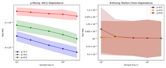
Figure 1. Experiment 1: Effect of dependence strength under $\alpha$-mixing (left) and $\Phi$-mixing (right). Curves show the mean test MSE over 100 repetitions, and the shaded region shows $\pm 1$ standard deviation. Stronger dependence leads to larger MSE, while the nearly parallel slopes confirm the theoretical rate $m^{-r/(2r+s)}$.

When plotted against $logm$, all curves decay almost linearly, indicating a power-law rate close to the theoretical $m^{-r/(2r+s)}$. That is, dependence modifies only the multiplicative constant while the convergence rate remains unchanged. Although AR(1) processes and finite-state Markov chains generate different types of temporal dependence ($\alpha$-mixing versus $\Phi$-mixing), both exhibit identical qualitative behavior: stronger dependence increases the finite-sample error but does not alter the asymptotic decay rate. This supports the generality of our theory across multiple dependence frameworks.

The tuning parameters $({\lambda }_m,h_m)$ depend solely on $(r,s,p)$ and do not use any information about the mixing strength. The smooth decay of all curves, despite very different dependence scenarios, demonstrates the practical robustness of this theoretically motivated choice. The parallel slopes in all settings show that the proposed estimator remains stable across a wide range of temporal dependence strengths. Thus, even in moderately or strongly dependent environments, the method retains its theoretical convergence behavior and delivers reliable empirical performance.

4.2. Experiment 2: Effect of the Number of Machines

In this experiment we investigate the scalability of the proposed distributed robust regression estimator as the number of machines increases. We fix the total sample size at

$$m=10000,$$

and the data follow the AR(1) model with dependence level $\varphi =0.6$. The number of machines is varied over

$$k\in \{1,2,3,4,5,6,10,15,20\}.$$

According to Theorem 1, the distributed estimator remains minimax optimal only if k grows no faster than

$$k_{max}\asymp m^{(2r+s-2)/(4r+2s)},$$

which equals approximately $2.5$ under our choice $r=1$ and $s=1/2$. When k exceeds this threshold, the local sample size $m/k$ becomes too small to guarantee the stability of the bias and variance terms.

Figure 2 exhibits a clear phase transition: the MSE remains nearly flat for $k=1$ and $k=2$, both of which lie below the predicted upper bound. Once k exceeds $k_{max}$, the error begins to increase and becomes unstable. This is consistent with the theoretical constraint that guarantees statistical optimality only when each local machine receives sufficiently many samples. For large values of k, each local machine receives only $m/k$ observations (e.g., only 500 samples when $k=20$). In this regime, the local estimators become significantly more variable, and the averaging step cannot adequately correct for the inflated variance. The resulting oscillatory behavior in the curve reflects precisely this high-variance effect.

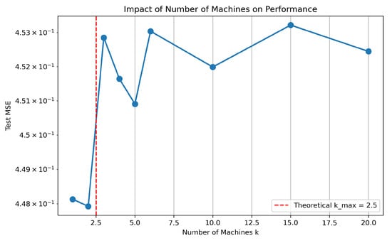
Figure 2. Experiment 2: Test MSE as a function of the number of machines k. The red dashed line marks the theoretical upper limit $k_{max}\approx 2.5$. Test error remains stable up to $k=2$ and begins to fluctuate and increase once $k>k_{max}$, in accordance with the theoretical prediction.

The experiment provides a direct empirical confirmation of the theoretical scalability bound: distributing the data across too many machines degrades performance even when the total number of samples is fixed. The fact that the degradation occurs almost exactly beyond the predicted threshold demonstrates that the bound $k_{max}$ is not merely an artifact of the analysis but accurately characterizes the practical limitation of distributed learning under dependence. The results highlight an important guideline for real-world implementations: to preserve minimax optimality, the number of computational workers must be chosen in accordance with the problem’s smoothness $\left(r\right)$ and marginal dimension $\left(s\right)$. The experiment confirms that over-parallelization can harm statistical efficiency, especially in the presence of temporal dependence.

5. Conclusions

Non-Gaussian noise and dependent samples are two stylized features of big data. In this paper we studied the learning performance of distributed robust regression with $\alpha$-mixing and $\varphi$-mixing inputs. Our analysis provides very useful information on the application of distributed kernel-sounding algorithms. It tells us that the number of local machines and robustification parameter should be selected according to the big sample size and mixing coefficients. It is worth mentioning that the selection of the robustification parameter should balance between the learning rates and the degree of robustness.

We should point out that integral operator decompositions are mostly used to analyze ordinary least-squares methods, where the loss functions are convex and derivatives of losses have a linear structure. However, the robust losses in this work are generally not convex and their derivatives do not have linear structures, which brings about essential difficulties in the technical analysis. Therefore, we introduce the robust error term to deal with the technical difficulty caused by non-convexity features of robust algorithms. We notice that the robust error term is vital in analyzing the learning performance of robust algorithms, as shown in Theorems 1 and 2. It helps us understand the difference between robust learning and OLS and explains that robust loss can completely reject gross outliers while keeping a prediction accuracy similar to that of least-squares losses.

References

- Feng, Y.; Wu, Q. Learning under (1+ϵ)-moment conditions. Appl. Comput. Harmon. Anal. 2020, 49, 495–520. [Google Scholar] [CrossRef]
- Ganan, S.; McClure, D. Bayesian image analysis: An application to single photon emission tomography. Amer. Statist. Assoc. 1985, 12–18. [Google Scholar]
- Hampel, F. A general definition of qualitative robustness. Ann. Math. Stat 1971, 42, 1887–1896. [Google Scholar] [CrossRef]
- Huber, P.J. Robust Statistics; John Wiley & Sons: Hoboken, NJ, USA, 2004; Volume 523. [Google Scholar]
- Mizera, I.; Müller, C.H. Breakdown points of Cauchy regression-scale estimators. Stat. Probab. Lett. 2002, 57, 79–89. [Google Scholar] [CrossRef]
- Principe, J.C. Information Theoretic Learning: Renyi’s Entropy and Kernel Perspectives; Springer Science & Business Media: Berlin/Heidelberg, Germany, 2010. [Google Scholar]
- Sun, D.; Roth, S.; Black, M.J. Secrets of optical flow estimation and their principles. In Proceedings of the 2010 IEEE Computer Society Conference on Computer Vision and Pattern Recognition, San Francisco, CA, USA, 13–18 June 2010; pp. 2432–2439. [Google Scholar]
- Tukey, J.W. A survey of sampling from contaminated distributions. Contrib. Probab. Stat. 1960, 448–485. [Google Scholar]
- Wang, X.; Jiang, Y.; Huang, M.; Zhang, H. Robust variable selection with exponential squared loss. J. Am. Stat. Assoc. 2013, 108, 632–643. [Google Scholar] [CrossRef]
- Lin, S.B.; Guo, X.; Zhou, D.X. Distributed learning with regularized least squares. J. Mach. Learn. Res. 2017, 18, 1–31. [Google Scholar]
- Muckec, N.; Blanchard, G. Parallelizing spectrally regularized kernel algorithms. J. Mach. Learn. Res. 2018, 19, 1–29. [Google Scholar]
- Hu, T.; Wu, Q.; Zhou, D.X. Distributed kernel gradient descent algorithm for minimum error entropy principle. Appl. Comput. Harmon. Anal. 2020, 49, 229–256. [Google Scholar] [CrossRef]
- Guo, Z.; Shi, L.; Wu, Q. Learning Theory of Distributed Regression with Bias Corrected Regularization Kernel Network. J. Mach. Learn. Res. 2017, 18, 1–25. [Google Scholar]
- Shi, L. Distributed learning with indefinite kernels. Anal. Appl. 2020, 17, 947–975. [Google Scholar] [CrossRef]
- Ouakrim, Y.; Boutaayamou, I.; Yazidi, Y.; Zafrar, A. Convergence analysis of an alternating direction method of multipliers for the identification of nonsmooth diffusion parameters with total variation. Inverse Probl. 2023, 39. [Google Scholar] [CrossRef]
- Liu, J.; Shi, L. Distributed learning with discretely observed functional data. Inverse Probl. 2025, 41. [Google Scholar] [CrossRef]
- Jiao, Y.; Yang, K.; Song, D. Distributed Distributionally Robust Optimization with Non-Convex Objectives. In Proceedings of the 36th Conference on Neural Information Processing Systems (NeurIPS), New Orleans, LA, USA, 28 November–9 December 2022. [Google Scholar]
- Allouah, Y.; Guerraoui, R.; Gupta, N.; Pinot, R.; Rizk, G. Robust Distributed Learning: Tight Error Bounds and Breakdown Point under Data Heterogeneity. In Proceedings of the 37th Conference on Neural Information Processing Systems (NeurIPS), New Orleans, LA, USA, 10–16 December 2023. [Google Scholar]
- Fan, J.; Liao, Y.; Liu, H. An overview of the estimation of large covariance and precision matrices. Econom. J. 2016, 19, C1–C32. [Google Scholar] [CrossRef]
- Sun, Q.; Zhou, W.X.; Fan, J. Adaptive Huber Regression. J. Am. Stat. Assoc. 2017, 115, 254–265. [Google Scholar] [CrossRef]
- Sun, H.; Wu, Q. Regularized least square regression with dependent samples. Adv. Comput. Math. 2010, 32, 175–189. [Google Scholar] [CrossRef]
- Sun, Z.; Lin, S.B. Distributed Learning with Dependent Samples. Inf. Theory IEEE Trans. (T-IT) 2022, 68, 6003–6020. [Google Scholar] [CrossRef]
- Li, L.; Wan, C. Support Vector Machines with Beta-Mixing Input Sequences. In International Symposium on Neural Networks; Springer: Berlin/Heidelberg, Germany, 2006. [Google Scholar]
- Mirzaei, E.; Maurer, A.; Kostic, V.R.; Pontil, M. An Empirical Bernstein Inequality for Dependent Data in Hilbert Spaces and Applications. In Proceedings of the 28th International Conference on Artificial Intelligence and Statistics, Mai Khao, Thailand, 3–5 May 2025. [Google Scholar]
- Agarwal, A.; Duchi, J.C. The Generalization Ability of Online Algorithms for Dependent Data. IEEE Trans. Inf. Theory 2011, 59, 573–587. [Google Scholar] [CrossRef]
- Modha, D.S.; Masry, E. Minimum complexity regression estimation with weakly dependent observations. IEEE Trans. Inf. Theory 2002, 42, 2133–2145. [Google Scholar] [CrossRef]
- Aronszajn, N. Theory of reproducing kernels. Trans. Am. Math. Soc. 1950, 68, 337–404. [Google Scholar] [CrossRef]
- Blanchard, G.; Mücke, N. Optimal Rates for Regularization of Statistical Inverse Learning Problems. Found. Comput. Math. 2016, 18, 971–1013. [Google Scholar] [CrossRef]
- Smale, S.; Zhou, D.X. Learning Theory Estimates via Integral Operators and Their Approximations. Constr. Approx. 2007, 26, 153–172. [Google Scholar] [CrossRef]
Disclaimer/Publisher’s Note: The statements, opinions and data contained in all publications are solely those of the individual author(s) and contributor(s) and not of MDPI and/or the editor(s). MDPI and/or the editor(s) disclaim responsibility for any injury to people or property resulting from any ideas, methods, instructions or products referred to in the content. |
© 2025 by the authors. Licensee MDPI, Basel, Switzerland. This article is an open access article distributed under the terms and conditions of the Creative Commons Attribution (CC BY) license (https://creativecommons.org/licenses/by/4.0/).