A Two-Stage Stochastic Optimization Model for Cruise Ship Food Provisioning with Substitution

Abstract

The global cruise industry has demonstrated remarkable growth, with modern ships functioning as large-scale floating resorts. Effective food provisioning is a critical operational function that directly impacts both cost efficiency and passenger satisfaction. This task is characterized by massive consumption scales and high demand uncertainty. To address these challenges, this paper develops a two-stage stochastic optimization model for cruise ship food provisioning. The first-stage decisions involve procurement quantities made before the voyage under demand uncertainty, subject to the volumetric constraints of different storage types. The second-stage decisions determine the optimal substitution plan after the actual demand is realized, mitigating shortages by utilizing alternative available items. Solving stochastic programs with continuous distributions is computationally challenging. Therefore, we employ the sample average approximation (SAA) method to obtain tractable solutions, complemented by a full statistical evaluation of solution quality. Numerical experiments using real-world data confirm that a scenario size of 80 achieves an optimal balance with an optimality gap of 0.78%. Sensitivity analysis demonstrates the model’s robust performance and provides valuable managerial insights: higher shortage penalty coefficients significantly reduce stockouts; two-way substitution structures enhance system flexibility; appropriate salvage value accounting reduces total costs; and implementing a service level constraint of ${\lambda }_i=0.80$ optimally balances operational resilience with economic efficiency. These findings support the development of more resilient and cost-effective provisioning strategies, offering cruise operators a practical decision-support tool for managing food provisioning under uncertainty.

1. Introduction

Over the past two decades, the global cruise industry has demonstrated remarkable growth dynamics, emerging as one of the most rapidly developing segments in the worldwide tourism market [1,2,3]. Nevertheless, cruise tourism continues to receive limited attention in academic research, representing a notably under-investigated area within tourism studies [4,5]. The quantity of studies focusing on cruise tourism remains disproportionately low, especially when contrasted with the extensive body of literature devoted to tourism in general [6]. Positioned as an applied discipline, research in this field has predominantly concentrated on analyzing industry evolution and enhancing operational frameworks [7,8]. Within this context, food provisioning management deserves particular emphasis due to the massive scale of consumption and high demand uncertainty characteristic of cruise operations. Optimized provisioning strategies not only substantially impact operational profitability but also contribute significantly to waste reduction objectives [9].

Food and beverage provisioning represents a critical operational function that directly impacts both cost efficiency and passenger satisfaction. Modern cruise ships have evolved into “floating resorts”, where dining experiences constitute a fundamental component of the overall vacation value proposition [10]. The scale of this challenge is substantial, as a single large cruise vessel must provision thousands of diverse food items for thousands of passengers and crew across extended voyages, all within the constraints of specialized storage facilities with limited capacities [11,12].

Making plans for all kinds of consumption during the voyage is a critical support of maritime operations [13,14,15]. A central aspect of this support involves the provisioning of food and beverages, which requires meticulous planning prior to departure due to limited onboard storage capacity and the inherent uncertainty in consumption patterns during voyages. Traditional deterministic planning methods, which rely on average demand forecasts, frequently result in either costly overstocking or problematic shortages [16,17]. The latter scenario is particularly critical, as it can adversely affect passenger satisfaction and overall operational effectiveness. At the same time, it is essential to consider how potential shortages of specific food categories during voyages should be proactively addressed through contingency planning.

Several studies have investigated cruise ship provisioning and related inventory management problems, employing various methodologies, as summarized in Table 1. Erkoc et al. [18] developed a multistage inventory replenishment model for cruise ship food and beverage provisioning, employing stochastic dynamic programming to optimize a three-stage procurement strategy that includes advance contracting, pre-departure expedited replenishment, and mid-voyage restocking, while demonstrating that optimal replenishment follows base-stock policies at each stage. However, its decision making is based on realized demand values rather than simultaneously formulating recourse actions for multiple potential demand scenarios within a unified stochastic programming framework, and it does not address effective response mechanisms—such as product substitution—for in-voyage stockouts. Véronneau and Roy [8] presented an empirical study of global cruise operations, examining supply chain management practices and challenges under dynamic supply point environments and summarizing key characteristics and managerial experiences in strategic planning, procurement processes, and port turnaround efficiency. Nevertheless, it primarily offers qualitative descriptions of managerial practices and operational challenges without developing mathematical models to quantitatively analyze optimal decisions under uncertainty or systematically addressing demand fluctuation and supply risks through stochastic optimization or inventory theory. Furthermore, while several studies in the supply chain risk management literature have explored just-in-time (JIT) replenishment strategies as potential solutions [19,20], they generally lack quantitative optimization frameworks that provide actionable decision support under uncertainty.

Table 1. Summary of the literature on cruise ship provisioning and related methodologies.

Study	Methodology	Limitations
Erkoc et al. [18]	Multistage inventory replenishment model; Stochastic dynamic programming	Decision-making based on realized demand; No substitution mechanisms; No unified stochastic programming framework
Véronneau and Roy [8]	Empirical study; Qualitative analysis of supply chain practices	No mathematical models; No quantitative optimization under uncertainty
Zhou et al. [19]	Supply chain risk management; Risk typology classification	Lacks quantitative optimization; No specific decision support tools
Meng and Wu [20]	Risk analysis; Set pair analysis–Markov chain model	Focuses on risk assessment rather than operational optimization
Pasternack and Drezner [21]	Stochastic inventory models; Substitutable products	General inventory context; Not tailored to cruise operations
Nagarajan and Rajagopalan [22]	Inventory models; Substitutable products	No cruise-specific constraints; Limited to moderate substitution levels
Ahiska and Kurtul [23]	Hybrid manufacturing-remanufacturing; Markov decision processes	Manufacturing context; Not applicable to cruise provisioning
Rao et al. [24]	Multiproduct systems; Two-stage stochastic programming	Industrial-scale focus; No cruise-specific considerations
Kim and Bell [25]	Joint pricing and production; Inventory-driven substitution	General retail context; No storage constraints consideration

To address these research gaps, we model the food provisioning problem as a two-stage stochastic program. The first-stage decisions are made before the voyage under demand uncertainty. They determine the optimal quantity of each food type to purchase. These decisions are subject to the volumetric constraints of different storage facilities, such as freezer, refrigerator, and ambient stores. The second-stage decisions are made after the actual demand is realized. They determine the optimal substitution plan to minimize penalty costs. This plan mitigates the shortage of one food item by using alternative available items. The overall objective is to minimize the total expected cost. This cost includes procurement costs, shortage penalties, substitution penalties, and salvage values. Solving stochastic programs with continuous distributions is computationally difficult. Therefore, we apply the sample average approximation (SAA) method. This method uses a finite set of generated demand scenarios to obtain tractable and high-quality solutions.

This paper presents three primary contributions to cruise ship logistics and stochastic optimization:

• We propose a two-stage stochastic optimization model for cruise ship food provisioning. It captures both demand uncertainty and food substitution. The model combines first-stage procurement decisions with second-stage recourse actions. This allows optimal substitution after demand is realized. Our approach minimizes expected costs and offers a practical decision-support tool.
• We solve the stochastic program using the SAA method. Our solution includes a full statistical evaluation of its quality. We establish a statistical lower bound by solving multiple independent SAA problems. We also compute an upper bound by evaluating candidate solutions on a large reference sample. The optimality gap is then estimated from these bounds. This ensures computational tractability and reliability for real-world, large-scale planning.
• We perform extensive sensitivity analyses to derive managerial insights. The results reveal that a higher shortage penalty coefficient leads to a significant reduction in stockouts, while accounting for food salvage value contributes to a reduction in the total cost. Based on these findings, we recommend that cruise operators implement two key strategies: first, adopt a substitution cost structure that permits two-way substitution, as this enhances system flexibility and rationalizes procurement; second, implement a service level constraint of approximately ${\lambda }_i=0.80$, as this setting optimally balances substitution flexibility with cost control, enhancing both operational resilience and economic efficiency.

The remainder of this paper is organized as follows. Section 2 provides a comprehensive review of the relevant literature. Section 3 details the problem description and presents the two-stage stochastic programming formulation alongside its SAA counterpart. Section 4 presents numerical experiments based on real-world data, including convergence analysis and sensitivity analyses. Section 5 discusses the practical implications of our research findings for cruise operators. Finally, Section 6 concludes with a summary of findings and potential future research directions.

2. Literature Review

Effective food and beverage provisioning constitutes a critical operational function in cruise management, characterized by distinctive storage constraints, substantial demand uncertainty, and the essential requirement of reducing stock shortages. This literature review synthesizes pertinent research from two interconnected domains. The analysis first examines the operational specificities and documented challenges within cruise ship food provisioning to establish the problem domain. Subsequent investigation focuses on the methodological foundations of stochastic inventory models incorporating substitution mechanisms, evaluating their potential applicability and inherent limitations for maritime operational environments.

2.1. The Operation Management Related to Food Provisioning on Cruise Ships

Efficient food provisioning represents a critical operational function in cruise ship management, directly impacting cost control and inventory control [26]. A fundamental challenge in this context arises from the significant uncertainty in passenger demand for various food items, which stems from multiple factors including fluctuating passenger counts, diverse demographic profiles with differing culinary preferences, and external variables such as itinerary changes and weather conditions [27,28].

Research on demand uncertainty reveals both seasonal patterns and risk factors that affect provisioning. Bo et al. [29] investigated Mediterranean cruise port seasonality by classifying temporal patterns into three distinct categories while demonstrating the crucial influence of maritime factors such as multisea complementary cruising and port hierarchy. Similarly, Fernández-Morales et al. [30] analyzed UK tourism seasonality using a decomposition approach, revealing varying patterns across market segments and advocating for disaggregated mitigation strategies. Beyond seasonal variations, Diabat et al. [31] identified demand-side risks as major supply chain threats originating from volatile consumption and sudden preference shifts, thereby necessitating provisioning strategies that address broader uncertainty spectra. It is worth noting that our problem differs fundamentally from high-dimensional transportation problems [32,33]. While the latter excel at optimizing spatial flows in deterministic networks, our focus is on sequential decision-making under uncertainty.

Studies specifically addressing cruise food provisioning employ diverse methodological approaches. Erkoc et al. [18] examined multistage replenishment through a stochastic model that optimizes contracting and inventory policies by integrating advance purchasing with expedited port replenishment, demonstrating base-stock policy optimality. In contrast, Veronneau and Roy [8] adopted an empirical perspective through field study methodology, identifying key operational characteristics and best practices in global service supply chains while emphasizing resupply complexities.

The literature on cruise supply chain challenges further enriches our understanding. Zhou et al. [19] developed a comprehensive risk typology that classifies vulnerabilities into four categories—macro risks, safety–security–health risks, information risks, and supply risks—providing a systematic framework for risk identification. Meng and Wu [20] employed a set pair analysis–Markov chain model to evaluate China’s cruise supply chain risks, forecasting evolution trends and potential provisioning stability disruptions. Although Sun et al. [34] primarily focused on marketing optimization, they acknowledged the persistent scarcity of operational research despite the industry’s rapid growth.

Complementing these perspectives, Li and Wang [9] investigated food waste among Chinese cruise passengers through qualitative methodology, revealing how cultural factors, passenger demographics, and all-inclusive pricing models significantly drive waste generation, thereby emphasizing the importance of avoiding excessive purchasing.

In summary, while the existing literature addresses individual aspects, including strategic inventory replenishment, practical supply chain management, and post-consumption analysis, it lacks a holistic approach. A unified optimization framework that simultaneously integrates demand uncertainty, operational constraints, and recourse actions such as substitution remains undeveloped, representing a significant gap in current research.

2.2. Stochastic Inventory Models with Substitution

The literature on inventory management for substitutable products provides valuable methodologies for handling demand uncertainty. Foundational work by Pasternack and Drezner [21] established the concavity of the expected profit function for two substitutable products, demonstrating that optimal order quantities are influenced by substitution revenue. Building on this, Rao et al. [24] developed a two-stage stochastic programming model for multiproduct systems with downward substitution and setup costs, providing effective heuristics for industrial-scale problems. Nagarajan and Rajagopalan [22] further analyzed optimal policies for substitutable products, showing that partially decoupled base-stock policies perform well when substitution levels are moderate. More recent contributions include Ahiska and Kurtul [23], who examined one-way substitution in hybrid manufacturing–remanufacturing systems using Markov decision processes, revealing that substitution remains profitable even with negative unit margins due to savings in lost sales. Finally, Kim and Bell [25] integrated both price-driven and inventory-driven substitution, developing joint pricing and production models that demonstrate how firms can leverage substitution to increase profitability. While these models provide robust frameworks for handling substitution in various contexts, their application to cruise ship food provisioning—with its unique combination of storage constraints, multiple substitution relationships, and voyage-length planning horizon—remains unexplored.

On the methodological front, these existing models exhibit important limitations in addressing the specialized requirements of cruise operations. Specifically, they fail to account for the distinctive challenges of cruise ship food provisioning, particularly the presence of specialized storage constraints and the need to manage complex substitution networks simultaneously across extended voyage durations. These methodological gaps motivate our research to develop a two-stage stochastic optimization model specifically designed for cruise operations. Our proposed model explicitly incorporates volumetric storage constraints and handles multiple substitution relationships, thereby providing a tailored decision-support framework for cruise ship food provisioning under uncertainty.

2.3. Research Gap

The synthesis of the existing literature reveals several critical gaps that this research aims to address in the domain of cruise ship food provisioning.

First, while prior studies have separately examined inventory replenishment and supply chain challenges in cruise operations, they often lack a holistic optimization framework. There is a notable absence of models that can simultaneously integrate proactive procurement decisions made under demand uncertainty with reactive recourse actions. Specifically, the literature lacks a unified stochastic programming paradigm that effectively combines first-stage purchasing decisions with the second-stage operational flexibility provided by product substitution strategies [35,36]. Although some stochastic optimization studies have explored substitution in multiproduct inventory systems, they have not been extended to the cruise provisioning context, where the combination of uncertainty, perishability, and voyage constraints presents unique modeling challenges [37,38].

Second, although the theory of inventory management for substitutable products is well established in general [22,39], existing models are not adequately tailored to the unique operational environment of a cruise ship. These models typically fail to account for the complex network of substitution relationships governed by nutritional value and taste similarity. Furthermore, they overlook the distinct volumetric constraints of frozen, refrigerated, and ambient storage, as well as the extended planning horizon of a voyage without port calls. Consequently, the direct application of these generic models to the cruise context inevitably yields suboptimal and impractical solutions [11,37].

Third, from a methodological standpoint, there is a clear need for a computationally tractable and statistically rigorous solution approach tailored for this class of large-scale stochastic optimization problems in maritime logistics. Many existing studies do not provide sufficient quality guarantees for their obtained solutions, limiting their practical utility. To bridge this gap, this paper employs the SAA method, which is complemented by a comprehensive statistical evaluation procedure. This procedure establishes tight lower and upper bounds on the optimal solution value, thereby ensuring the reliability and practical applicability of the proposed provisioning strategy for real-world decision making [36,40].

3. Problem Formulation

3.1. Problem Description

The operation of a large commercial cruise ship is characterized by extended voyages far from port and the need to provide consistent, high-quality dining experiences for thousands of passengers and crews. This imposes significant challenges for food provisioning, as the ship must carry vast quantities of diverse food items to meet consumption demands until the next port of call.

The notation used is shown in Table 2. The limited and specialized storage capacities on board—categorized into frozen, refrigerated, and ambient stores—further complicate logistics. Each storage type $k\in K$ has a finite volumetric capacity $Q_k$ (cubic meters). Each food item $i\in N$ (e.g., beef, lettuce, milk) has a specific unit volume $v_i$ (cubic meters per kg) and can only be stored in its compatible storage types $K_i\subseteq K$.

Table 2. Notations used in the model formulation.

Symbol	Description
Sets
N	Set of food types
K	Set of storage capacity types (e.g., frozen, refrigerated, ambient)
$K_i\subseteq K$	Set of storage types suitable for food item $i\in N$
$N_i\subseteq N\setminus \left\{i\right\}$	Set of food items that can substitute for food item $i\in N$
$H_k$	Set of foods that can be stored in storage capacity types $k\in K$
Parameters
$c_i$	Unit procurement cost for food $i\in N$
$v_i$	Unit volume of food $i\in N$
$s_i$	Unit salvage value for surplus of food $i\in N$
$p_i$	Unit penalty cost for shortage of food $i\in N$
$d_{ij}$	Unit penalty cost for substituting 1 kg of i with $j\in N_i$
$q_{ij}$	Quantity of food j required to substitute for 1 kg of food i
$Q_k$	Total volume capacity of storage type $k\in K$
${\xi }_i$	Random variable representing demand for food $i\in N$
$S_i^0$	Initial shortage of food i before substitution $i\in N$
$R_i^0$	Initial surplus of food i before substitution $i\in N$
${\lambda }_i$	Service level parameter for food item $i\in N$
Decision Variables
First-Stage Variables
$x_i$	Total quantity of food i purchased $i\in N$
$x_{ik}$	Quantity of food i to purchase and store in capacity type $k\in K_i$
Second-Stage Variables
$u_{ij}$	Amount of shortage of food i fulfilled by substitute $j\in N_i$
$w_i$	Final leftover quantity (surplus) of food item i after substitution

The provisioning manager faces a two-stage decision process. In the first stage, before the voyage begins, the manager must determine the total quantity $x_i$ of each food item $i\in N$ to procure, considering the procurement cost $c_i$ per unit. These food items are then allocated to specialized storage compartments on board, where $x_{ik}$ denotes the quantity of food i stored in compartment type $k\in K_i$.

The exact consumption (demand) for each food item during the voyage, denoted by the random variable ${\tilde{\xi }}_i$, cannot be known with certainty in advance. This uncertainty stems from factors such as fluctuating passenger counts, changing weather conditions affecting appetites, and varying menu preferences. We can obtain the distribution of the data by using statistical methods such as drawing frequency distribution histograms based on historical data.

After demand realization in the second stage, the initial shortage $S_i^0=\max (0,{\xi }_i-x_i)$ and initial surplus $R_i^0=\max (0,x_i-{\xi }_i)$ are observed. If the demand for a particular food item i exceeds the loaded quantity, a shortage occurs. To mitigate the impact of shortages, the cruise line has established a substitution protocol. For each food item i, there exists a set of predefined substitute items $N_i\subseteq N\setminus i$. For example, if beef (i) is unavailable, pork ($j\in N_i$) may be used as a substitute. However, this substitution is imperfect; it requires $q_{ij}$ kilograms of substitute j to replace 1 kg of the original item i and incurs a penalty cost $d_{ij}$, reflecting the perceived quality drop and potential passenger dissatisfaction. The substitution amount is denoted by $u_{ij}$. It is important to emphasize that substitution does not create additional inventory but serves as a risk response strategy after shortages are identified, utilizing similar products as supplements. If a shortage is not substituted, a penalty $p_i$ is incurred per unit of unmet demand $S_i^0-{\sum }_{j\in N_i}{u}_{ij}$. A service level parameter ${\lambda }_i$ is introduced for each food item i to represent the minimum proportion of demand that must be fulfilled by the original product, with the maximum allowable substitution proportion thus being $(1-{\lambda }_i)$.

After the voyage, any remaining food i, denoted by $w_i$, has a salvage value $s_i$ per unit, which could be positive (if it can be used on the next voyage) or negative (if it requires costly disposal).

The provisioning manager aims to minimize the total expected cost. This includes the initial procurement cost at the home port and the expected costs arising during the voyage—namely, shortage penalties, substitution penalties, and negative salvage revenue (or plus salvage income). Therefore, the decisions of how much of each food type to load must be made wisely, considering the uncertain demand and the available recourse through substitution, with the aim of ensuring supply continuity and cost-effectiveness for the cruise operation.

3.2. Model Formulation

3.2.1. Two-Stage Stochastic Programming Formulation

The problem is formulated as the following two-stage stochastic program.

First-Stage Problem:

$$\begin{array}{cc}\hfill \min & \sum _{i\in N}\sum _{k\in K_i}{c}_i{x}_{ik}+{\mathbb{E}}_{\mathit{\xi }}\left[C(\mathbf{x},\mathit{\xi })\right]\hfill \end{array}$$

(1)

$$\begin{array}{cc}\hfill \mathrm{s}.\mathrm{t}.& \sum _{i\in H_k}{v}_i{x}_{ik}\le Q_k,\forall k\in K\hfill \end{array}$$

(2)

$$\begin{array}{cc}\hfill & x_i=\sum _{k\in K_i}{x}_{ik},\forall i\in N\hfill \end{array}$$

(3)

$$\begin{array}{cc}\hfill & x_{ik}\ge 0,\forall i\in N,\forall k\in K_i.\hfill \end{array}$$

(4)

The mathematical model formulated above represents the first-stage problem of a two-stage stochastic programming framework. The objective function (1) aims to minimize the total expected cost. The $C(\mathbf{x},\mathit{\xi })$ represents the cost in the second stage when the random variable takes the value of $\mathit{\xi }$. Constraint (2) ensures that the total volume of all food items assigned to each storage type k does not exceed its respective capacity $Q_k$. Constraint (3) ensures that the storage quantity in different storage types is equal to the purchase quantity. Finally, constraint (4) enforces the non-negativity of the first-stage decision variables $x_{ik}$.

Second-Stage Problem: For a given realization $\mathit{\xi }=({\xi }_1,\dots ,{\xi }_{\left|N\right|})$ of demand, we define the initial shortage and surplus as parameters:

$$\begin{array}{cc}\hfill S_i^0& =\max (0,{\xi }_i-x_i),\forall i\in N\hfill \end{array}$$

(5)

$$\begin{array}{cc}\hfill R_i^0& =\max (0,x_i-{\xi }_i),\forall i\in N.\hfill \end{array}$$

(6)

The second-stage problem $C(\mathbf{x},\mathit{\xi })$ is

$$C(\mathbf{x},\mathit{\xi })=\min \sum _{i\in N}{p}_i(S_i^0-\sum _{j\in N_i}{u}_{ij})-\sum _{i\in N}{s}_i{w}_i+\sum _{i\in N}\sum _{j\in N_i}{d}_{ij}{u}_{ij}$$

(7)

$$\mathrm{s}.\mathrm{t}.\sum _{j\in N_i}{u}_{ij}\le S_i^0,\forall i\in N$$

(8)

$$\sum _{j:i\in N_j}{q}_{ji}{u}_{ji}\le R_i^0,\forall i\in N$$

(9)

$$w_i=R_i^0-\sum _{j:i\in N_j}{q}_{ji}{u}_{ji}+\sum _{j\in N_i}{u}_{ij},\forall i\in N$$

(10)

$$\sum _{j\in N_i}{u}_{ij}\le (1-{\lambda }_i)·{\xi }_i,\forall i\in N$$

(11)

$$u_{ij}\ge 0,\forall i\in N,\forall j\in N_i$$

(12)

$$w_i\ge 0,\forall i\in N.$$

(13)

The second-stage model is defined after the observation of the specific demand realization $\mathit{\xi }$. Constraints (5) and (6) calculate initial shortage and surplus. The objective function (7) minimizes the total recourse cost. Constraint (8) guarantees that the total amount of food i replaced by its substitutes cannot exceed its initial shortage. Constraint (9) ensures that the total consumption of food i, when used as a substitute for other foods, does not exceed its initial surplus. Constraint (10) defines the final surplus of food i, $w_i$. To maintain service quality, Constraint (11) is introduced to limit the substitution quantity for each food item i to a maximum proportion $(1-{\lambda }_i)$ of its demand ${\xi }_i$. Finally, constraints (12) and (13) enforce the non-negativity of the decision variables $u_{ij}$ and $w_i$.

3.2.2. SAA Model

Let ${\mathit{\xi }}^s=({\xi }_1^s,\dots ,{\xi }_{\left|N\right|}^s)$ represent the demand vector in scenario s, for $s=1,\dots ,S$. The SAA model is

$$\begin{array}{cc}\hfill \min & \sum _{i\in N}\sum _{k\in K_i}{c}_i{x}_{ik}+{\displaystyle \frac{1}{S}}\sum _{s=1}^S{C}^s(\mathbf{x},{\mathit{\xi }}^s)\hfill \end{array}$$

(14)

$$\begin{array}{cc}\hfill \mathrm{s}.\mathrm{t}.& C^s(\mathbf{x},{\mathit{\xi }}^s)=\sum _{i\in N}{p}_i(S_i^{0s}-\sum _{j\in N_i}{u}_{ij}^s)-\sum _{i\in N}{s}_i{w}_i^s+\sum _{i\in N}\sum _{j\in N_i}{d}_{ij}{u}_{ij}^s,\forall s\in S\hfill \end{array}$$

(15)

$$\begin{array}{cc}\hfill & S_i^{0s}=\max (0,{\mathit{\xi }}_i^s-x_i),\forall s\in S\hfill \end{array}$$

(16)

$$\begin{array}{cc}\hfill & R_i^{0s}=\max (0,x_i-{\mathit{\xi }}_i^s),\forall s\in S\hfill \end{array}$$

(17)

$$\begin{array}{cc}\hfill & \sum _{i\in H_k}{v}_i{x}_{ik}\le Q_k,\forall k\in K\hfill \end{array}$$

(18)

$$\begin{array}{cc}\hfill & \sum _{j\in N_i}{u}_{ij}^s\le S_i^{0s},\forall i\in N,\forall s\in S\hfill \end{array}$$

(19)

$$\begin{array}{cc}\hfill & \sum _{j:i\in N_j}{q}_{ji}{u}_{ji}^s\le R_i^{0s},\forall i\in N,\forall s\in S\hfill \end{array}$$

(20)

$$\begin{array}{cc}\hfill & w_i^s=R_i^{0s}-\sum _{j:i\in N_j}{q}_{ji}{u}_{ji}^s+\sum _{j\in N_i}{u}_{ij}^s,\forall i\in N,\forall s\in S\hfill \end{array}$$

(21)

$$\begin{array}{cc}\hfill & \sum _{j\in N_i}{u}_{ji}^s\le (1-{\lambda }_i)·{\xi }_i,\forall i\in N,\forall s\in S\hfill \end{array}$$

(22)

$$\begin{array}{cc}\hfill & x_{ik}\ge 0,\forall i\in N,\forall k\in K_i\hfill \end{array}$$

(23)

$$\begin{array}{cc}\hfill & u_{ij}^s\ge 0,\forall i\in N,\forall j\in N_i,\forall s\in S\hfill \end{array}$$

(24)

$$\begin{array}{cc}\hfill & w_i^s\ge 0,\forall i\in N,\forall s\in S\hfill \end{array}$$

(25)

This formulation presents the SAA model, which is a deterministic equivalent of the original two-stage stochastic program. The core idea is to approximate the expected value of the second-stage cost by averaging over a finite set of S randomly generated demand scenarios.

The objective function (14) minimizes the total cost, comprising the first-stage procurement cost and the average second-stage recourse cost across all sampled scenarios. The second-stage function $C^s(\mathbf{x},{\mathit{\xi }}^s)$ in (15) calculates the cost for each scenario, including the shortage penalty, minus the salvage value, plus the substitution penalty. Equations (16) and (17) define the initial shortage and surplus for each scenario. Constraint (18) ensures that the total volume of food stored in each capacity type does not exceed its limit. Constraints (19) ensure that the total substitution for a food item does not exceed its initial shortage in each scenario. Constraints (20) ensure that the total consumption of a food item as a substitute does not exceed its initial surplus in each scenario. Constraints (21) define the final surplus of each food item after substitution. Constraint (22) is introduced to limit the substitution quantity for each food item i to a maximum proportion $(1-{\lambda }_i)$ of its demand ${\xi }_i$. Constraints (23) to (25) are the non-negativity constraints for the decision variables.

3.2.3. Linearized SAA Model

The max operators in (16) and (17) can be linearized using auxiliary binary variables and big-M constraints. The linearized constraints are

$$S_i^{0s}\ge {\xi }_i^s-x_i,\forall i\in N,\forall s$$

(26)

$$S_i^{0s}\ge 0,\forall i\in N,\forall s\in S$$

(27)

$$S_i^{0s}\le {\xi }_i^s-x_i+M(1-{\alpha }_i^s),\forall i\in N,\forall s\in S$$

(28)

$$S_i^{0s}\le M{\alpha }_i^s,\forall i\in N,\forall s\in S$$

(29)

$$R_i^{0s}\ge x_i-{\xi }_i^s,\forall i\in N,\forall s\in S$$

(30)

$$R_i^{0s}\ge 0,\forall i\in N,\forall s\in S$$

(31)

$$R_i^{0s}\le x_i-{\xi }_i^s+M(1-{\beta }_i^s),\forall i\in N,\forall s\in S$$

(32)

$$R_i^{0s}\le M{\beta }_i^s,\forall i\in N,\forall s\in S$$

(33)

$${\alpha }_i^s+{\beta }_i^s=1,\forall i\in N,\forall s\in S$$

(34)

$${\alpha }_i^s,{\beta }_i^s\in \{0,1\},\forall i\in N,\forall s\in S$$

(35)

where M is a sufficiently large constant, and ${\alpha }_i^s$, ${\beta }_i^s$ are binary variables. This linearization ensures that

-

If ${\xi }_i^s>x_i$ then ${\alpha }_i^s=1$, ${\beta }_i^s=0$, $S_i^{0s}={\xi }_i^s-x_i$, $R_i^{0s}=0$

-

If ${\xi }_i^s\le x_i$ then ${\alpha }_i^s=0$, ${\beta }_i^s=1$, $S_i^{0s}=0$, $R_i^{0s}=x_i-{\xi }_i^s$ thus exactly replicating the behavior of the original max operators.

3.2.4. Lower Bound

Let $z^{*}$ denote the true optimal objective value of the original stochastic program, and let ${\tilde{L}}_S$ be the optimal value of the SAA problem with sample size S. According to the statistical properties of SAA, we have

$$\mathbb{E}\left[{\tilde{L}}_S\right]\le z^{*}.$$

(36)

This establishes that the expected optimal value of the SAA problem provides a statistical lower bound for the true optimal value.

In practice, we solve T independent SAA problems, each with sample size S, obtaining optimal values $L_1,L_2,\dots ,L_T$. The sample average provides an estimate of the expected value:

$$\overline{L}={\displaystyle \frac{1}{T}}\sum _{t=1}^T{L}_t.$$

(37)

The sample standard deviation is calculated as

$$s_L=\sqrt{{\displaystyle \frac{1}{T-1}}{\displaystyle \sum _{t=1}^T}{(L_t-\overline{L})}^2}.$$

(38)

By the central limit theorem, when T is sufficiently large (typically $T\ge 30$), we can construct a $(1-\alpha )$ confidence lower bound:

$$LB=\overline{L}-t_{T-1,\alpha }{\displaystyle \frac{s_L}{\sqrt{T}}},$$

(39)

where $t_{T-1,\alpha }$ is the $(1-\alpha )$-quantile of the t-distribution with $T-1$ degrees of freedom. We are approximately $(1-\alpha )$ confident that $z^{*}\ge LB$.

3.2.5. Upper Bound

For any feasible first-stage solution ${\mathbf{x}}^{\mathrm{SAA}}$ obtained from the SAA procedure, the true expected cost provides an upper bound:

$$UB\left({\mathbf{x}}^{\mathrm{SAA}}\right)=\sum _{i\in N}\sum _{k\in K_i}{c}_i{x}_{ik}^{\mathrm{SAA}}+\mathbb{E}\left[C({\mathbf{x}}^{\mathrm{SAA}},\tilde{\mathit{\xi }})\right]\ge z^{*}.$$

(40)

In practice, we estimate this upper bound using a large reference sample $S^{\prime }$ with $|S^{\prime }|\gg S$:

$$\widehat{UB}=\sum _{i\in N}\sum _{k\in K_i}{c}_i{x}_{ik}^{\mathrm{SAA}}+{\displaystyle \frac{1}{|S^{\prime }|}}\sum _{s^{\prime }=1}^{|S^{\prime }|}C({\mathbf{x}}^{\mathrm{SAA}},{\mathit{\xi }}^{s^{\prime }}).$$

(41)

Due to the law of large numbers and the large size of $S^{\prime }$, $\widehat{UB}$ provides a high-quality estimate of the true upper bound.

3.2.6. Optimality Gap

The optimality gap of the SAA solution ${\mathbf{x}}^{\mathrm{SAA}}$ can be estimated as

$$\widehat{\mathrm{Gap}}=\max \left(0,\widehat{UB}-LB\right).$$

(42)

This gap provides a statistical guarantee on the quality of the obtained solution. A small gap indicates that the SAA solution is close to the true optimum.

3.2.7. Common Random Numbers for Variance Reduction

To obtain sharper bounds for the optimality gap, we employ the common random numbers (CRN) technique in both lower and upper bound estimations. As a well-established variance reduction method in simulation optimization, the CRN approach operates by using the same stream of random numbers across different system configurations [41]. The fundamental principle relies on introducing positive correlation between performance measures, thereby making their differences primarily reflect actual solution quality rather than random noise [42]. Let ${\mathit{\xi }}_{ts}$ denote the demand scenarios used in solving the T SAA problems ($t=1,\dots ,T$, $s=1,\dots ,S$). The stochastic upper bound is calculated as

$$\begin{array}{cc}\hfill \overline{U}& ={\displaystyle \frac{1}{TS}}\sum _{t=1}^T\sum _{s=1}^S\left[\sum _{i\in N}\sum _{k\in K_i}{c}_i{x}_{ik}^{\mathrm{SAA}}+C({\mathbf{x}}^{\mathrm{SAA}},{\mathit{\xi }}_{ts})\right]\hfill \end{array}$$

(43)

$$\begin{array}{cc}\hfill s_U& =\sqrt{{\displaystyle \frac{1}{TS-1}}{\displaystyle \sum _{t=1}^T}{\displaystyle \sum _{s=1}^S}{\left[\sum _{i\in N}\sum _{k\in K_i}{c}_i{x}_{ik}^{\mathrm{SAA}}+C({\mathbf{x}}^{\mathrm{SAA}},{\mathit{\xi }}_{ts})-\overline{U}\right]}^2}\hfill \end{array}$$

(44)

$$\begin{array}{cc}\hfill U{B}^{\mathrm{stoc}}& =\overline{U}+t_{TS-1,\alpha }{\displaystyle \frac{s_U}{\sqrt{TS}}}.\hfill \end{array}$$

(45)

Using common random numbers ensures that $U{B}^{\mathrm{stoc}}\ge LB$ with high probability, providing a more reliable optimality gap estimate.

4. Numerical Experiments

4.1. Parameter Settings

The parameter settings for this study are based on published data and official sources. The foundational data for food types and quantities required for large-scale cruise ship provisioning are derived from industry reports and journalistic investigations [43,44]. To ensure the accuracy of nutritional parameters, calorie and composition data are referenced from the USDA Food Composition Database [45] and other authoritative nutritional sources [46,47].

Table 3 presents the parameter settings for 14 major food items, including unit procurement cost $c_i$, unit volume $v_i$, calorie content, and the average amount of weekly demand.

Table 3. Food parameter settings.

Food Item	Unit Cost ${\mathit{c}}_{\mathit{i}}\left(\mathit{\$}\right)$	Unit Volume ${\mathit{v}}_{\mathit{i}}$ (m3/kg)	Calories	Weekly Demand (kg)
Eggs	8.10	0.0001	1310	1360.78
Chicken	20.67	0.0010	1825	1971.63
Beef	61.13	0.0010	1250	3089.44
Ice Cream	20.00	0.0005	2520	143.79
Potatoes	3.50	0.0008	805	4114.26
Flour	5.50	0.0006	3600	2592.80
Salmon	75.00	0.0012	2080	514.59
Lobster Tails	200.00	0.0020	970	432.22
French Fries	20.00	0.0008	2000	1028.73
Bacon	55.00	0.0010	2500	1088.89
Tortillas	10.00	0.0005	2370	2465.62
Chicken Wings	35.00	0.0010	2100	411.43
Coffee	125.00	0.0002	3200	308.59
Tea	200.00	0.0002	3300	308.59

The parameter configuration follows these principles: The shortage penalty cost $p_i$ is set at twice the procurement cost $c_i$ ($p_i=2c_i$), reflecting customer dissatisfaction and reputation impact caused by stockouts [48]. The salvage value $s_i$ is set at negative 10% of the procurement cost ($s_i=-0.1c_i$), representing the disposal cost for leftover food [49]. The service level parameter ${\lambda }_i$, which represents the maximum allowable proportion of demand that can be fulfilled through substitution, is uniformly set to 0.80 for all food items.

Substitution relationships are established considering nutritional value and taste similarity. The substitution cost $d_{ij}$ is set at 10% of the procurement cost of the substituted food item $c_i$ ($d_{ij}=0.1c_i$) [50,51]. The calorie substitution ratio $q_{ij}$ is calculated based on calorie content: $q_{ij}={\displaystyle \frac{\mathrm{Calories}\mathrm{of}\mathrm{food}i}{\mathrm{Calories}\mathrm{of}\mathrm{food}j}}.$

To ensure the economic rationality of substitution relationships within the optimization framework, two essential constraints are implemented. The substitution economic constraint, formulated as $p_i>d_{ij}$, requires that the direct substitution cost remains lower than the shortage penalty, thereby ensuring the economic advantage of substitution over unmet demand. The substitution feasibility constraint, expressed as $p_j·q_{ij}+d_{ij}>p_i$, prevents infinite arbitrage loops by ensuring that the total cost of substitution exceeds the original shortage penalty. Together with the service level constraint (11), these relationships prevent managers from obtaining erroneous optimization results due to inappropriate parameter settings in practical decision making. These constraints collectively guarantee that all permitted substitutions are both economically viable and operationally sound. Table 4 presents the validated substitution relationships that satisfy these conditions.

Table 4. Substitution relationship settings and constraint validation results.

Substituted Food	Substitute Food	Calorie Ratio ${\mathit{q}}_{\mathit{ij}}$	Substitution Cost ${\mathit{d}}_{\mathit{ij}}\left(\mathit{\$}\right)$
Chicken	Beef	1.460	2.07
	Salmon	0.877	2.07
Salmon	Beef	1.664	7.50
Potatoes	French Fries	0.403	0.35
Chicken Wings	Bacon	0.840	3.50
Coffee	Tea	1.000	12.50

After constraint validation, six substitution relationships satisfy the economic rationality conditions. The validation process eliminated economically infeasible substitutions where the total substitution cost ($p_j·q_{ij}+d_{ij}$) does not exceed the shortage penalty $p_i$ of the substituted food. This ensures that all remaining substitution decisions in the model meet both nutritional requirements and economic significance.

Notably, the validation results reveal asymmetric substitution patterns. For instance, while chicken can be substituted by beef and salmon, the reverse substitutions (beef by chicken, salmon by chicken) are eliminated due to economic infeasibility. If we maintain these substitution relationships, ultimately all the demand for beef will be met by chicken.

Based on actual cruise ship storage conditions, capacity constraints for three types of storage facilities are established [52,53]. Frozen storage provides 100 m³ capacity for ice cream, frozen meats, and other frozen items. Refrigerated storage offers 80 m³ capacity for fresh meats, dairy products, and other refrigerated items. Ambient storage maintains 50 m³ capacity for flour, potatoes, and other shelf-stable foods.

To ensure both numerical stability and computational efficiency in the large-M linearization formulation, the parameter M is carefully calibrated. To ensure numerical stability in the linearized constraints, the big-M constant is set to $M=100\times {\max }_{i\in N}\left(\mathbb{E}\left[{\xi }_i\right]\right)$, where $\mathbb{E}\left[{\xi }_i\right]$ is the mean demand for food item i. This unified calibration is justified as both auxiliary variables $S_i^{0s}$ and $R_i^{0s}$ are bounded by demand deviations from procurement quantities that are optimized around mean demands. The chosen M is sufficiently large to maintain constraint correctness under all plausible demand realizations, while avoiding numerical issues caused by excessively large values.

Passenger demand modeling is based on a cruise ship carrying 1500 passengers during a 7-day voyage. The demand for each food item is modeled as a normal distribution, an assumption supported by the central limit theorem given the large number of passengers (1500) and the aggregation of individual consumption patterns [54,55,56]. While we employ the normal distribution for computational tractability and scenario generation, the proposed optimization framework is robust to alternative demand distributions, as the SAA method relies only on demand scenarios rather than specific distributional assumptions [57,58]. The mean of the distribution is set equal to the historical weekly provisioning quantity listed in Table 3. The standard deviation is set at 10% of this mean value.

A Monte Carlo simulation with 3000 randomly generated scenarios comprehensively captures the demand uncertainty, ensuring the optimization model’s robustness and practical applicability to real-world operational environments.

4.2. Convergence Analysis

The algorithm uses Python 3.5 and runs on an x64-PC with a six-core Intel i7-12700H 2.3 GHz CPU and 16.0 GB of RAM. Gurobi 12 is used to solve the SAA model.

To determine the appropriate number of scenarios S for the SAA method, we conduct a convergence analysis of the solution results under different scenario sizes. The number of scenarios S is set to 10, 20, 30, 40, 60, 80, and 100, respectively. For each tested S, the statistical evaluation procedure is rigorously applied: we solve $T=30$ independent SAA problems to estimate the lower bound, ensuring the robustness of our expected value estimate. The upper bound is evaluated using a large reference sample of size $S^{\prime }=20\times S$, which guarantees that $S^{\prime }\gg S$ and provides a high-quality estimate of the true expected cost. All reported lower bounds, upper bounds, and standard deviations are derived from this procedure and are associated with a 95% confidence level, ensuring the statistical reliability of the reported optimality gaps and solution quality metrics.

The SAA algorithm is executed to solve the two-stage stochastic programming model, obtaining the upper and lower bounds of the objective value and statistical indicators, as shown in Table 5. The optimality gap in is calculated as follows: $Gap={\displaystyle \frac{UB-LB}{LB}}\times 100\%$.

Table 5. Decision results under different numbers of scenarios.

Number of Scenarios	Obj LB	Obj UB	Gap (%)	LB Std. Dev. (%)	UB Std. Dev. (%)	Time(s)
10	1,443,787.71	1,475,263.39	2.13	1.18	0.25	0.12
20	1,449,177.39	1,477,495.90	1.92	0.82	0.21	0.30
30	1,453,118.39	1,471,652.35	1.26	0.81	0.20	1.06
40	1,456,864.13	1,474,720.78	1.21	0.54	0.13	1.59
60	1,456,997.59	1,474,842.91	1.21	0.55	0.10	4.15
80	1,459,413.71	1,470,951.34	0.78	0.64	0.07	9.39
100	1,459,431.67	1,471,970.30	0.85	0.39	0.07	17.62

According to the results in Table 5, as the number of scenarios S increases, both the optimality gap and the standard deviations of the upper and lower bounds generally show a decreasing trend, indicating that increasing the number of scenarios can effectively improve solution quality. However, excessively increasing the number of scenarios will expand the problem scale, leading to increased computational time for the algorithm.

Considering both solution quality and computational efficiency, we select $S=80$ as the appropriate parameter setting for subsequent experiments. Although increasing the number of scenarios from 40 to 80 leads to a moderate increase in computational time (from 1.59 to 9.39 s), it provides a significant improvement in solution quality by reducing the optimality gap from 1.21% to 0.78%. The selection of $S=80$ offers an optimal balance between computational tractability and statistical precision for cruise ship food provisioning decisions. This scenario count provides robust protection against demand uncertainty while maintaining reasonable computational requirements, making it well suited for operational planning in maritime logistics contexts where both accuracy and timeliness are critical considerations.

4.3. Sensitivity Analysis

4.3.1. Sensitivity Analysis of Demand Variance

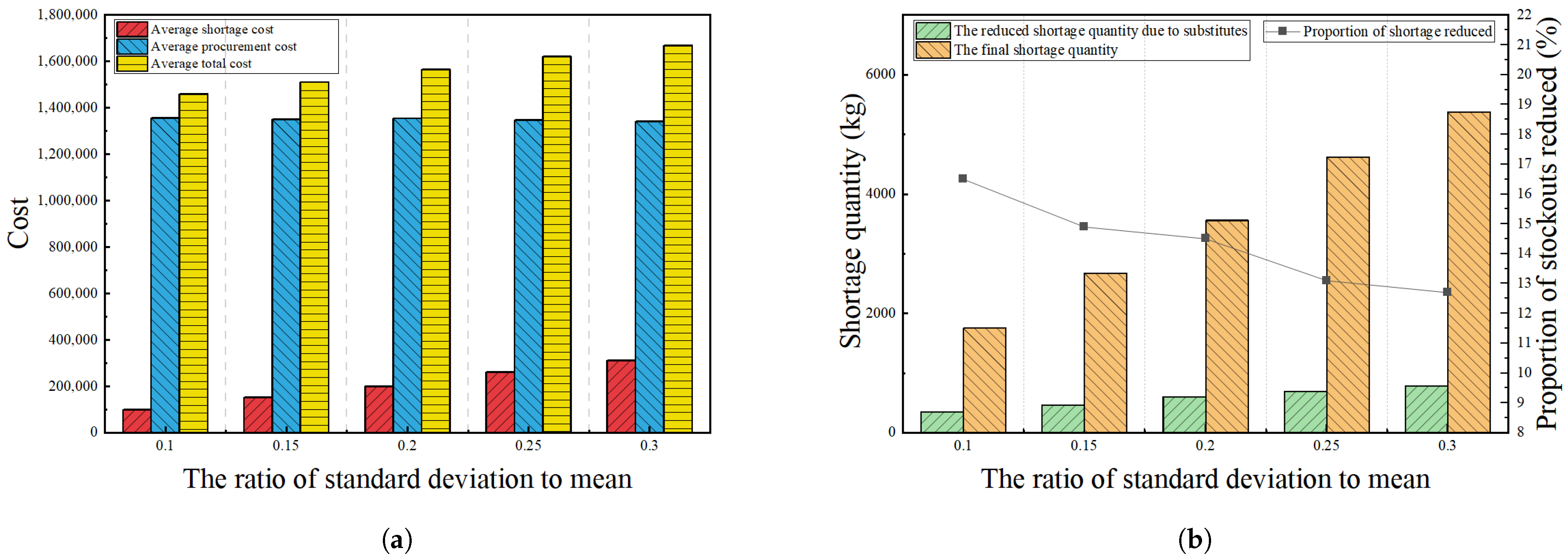
A sensitivity analysis is conducted to evaluate the impact of demand variance, expressed as the ratio of standard deviation to mean. As illustrated in Figure 1a, the average total cost and the average shortage cost both exhibit a clear upward trend as the variance increases from 0.1 to 0.3, indicating that higher uncertainty exacerbates stockout situations. In contrast, the purchasing cost demonstrates a noticeable decline under the same conditions. This phenomenon is clearly demonstrated in Figure 1b. As demand variance increases, the total shortage quantity rises significantly. However, the substitution mechanism effectively compensates for this by supplying additional items, offsetting approximately 12–17% of the shortage volume. Notably, as demand uncertainty increases, the substitution compensation quantity decreases correspondingly, primarily because each food item needs to reserve more inventory to cope with its own demand uncertainty, thereby reducing the surplus available for substitution. This complementary relationship underscores that while uncertainty increases costs and shortages, the adoption of a substitution strategy serves as an effective mitigation measure, reducing the reliance on traditional purchasing and enhancing model resilience against variability.

Figure 1. Impact of demand standard deviation on costs and substitution effectiveness. (a) Cost components under demand uncertainty. (b) Reduction in shortages achieved through substitution.

4.3.2. Sensitivity Analysis of Purchase Cost

The impact of procurement price fluctuations is analyzed by varying the purchase cost coefficient from 0.8 to 1.2. The results are summarized in Table 6. A clear positive correlation is observed between the purchase cost coefficient and the total cost. As the coefficient increases from 0.8 to 1.2, the total cost rises from 1,399,396.28 to 1,927,393.49, representing a 37.7% increase. This growth is primarily driven by the purchase cost component, which increases from 1,149,321.61 to 1,491,940.08. Concurrently, shortage cost shows a more pronounced upward trend, escalating from 230,791.79 to 424,120.86, indicating that higher procurement prices significantly exacerbate shortage situations by constraining purchasing capacity.

Table 6. Decision results under different purchase cost coefficients.

Purchase Cost Coefficient	Purchase Cost	Shortage Cost	Substitution Cost	Total Cost
0.8	1,149,321.61	230,791.79	1519.69	1,399,396.28
0.9	1,265,398.26	258,653.29	1638.12	1,541,743.47
1.0	1,343,974.79	316,122.14	1759.14	1,674,964.78
1.1	1,427,816.21	365,622.20	1883.24	1,806,612.59
1.2	1,491,940.08	424,120.86	1859.91	1,927,393.49

The quantity analysis shown in Table 7 reveals the underlying operational dynamics. As the purchase cost coefficient increases from 0.8 to 1.2, the total purchase quantity decreases from 44,745.11 kg to 38,912.81 kg, reflecting a rational cost-control response. This reduction in procurement has a direct consequence, leading to increased initial shortages that rise from 4894.04 kg to 8006.57 kg. The substitution quantity demonstrates a decreasing trend, declining from 843.22 kg to 653.52 kg, suggesting that higher purchase costs limit the economic feasibility of certain substitution options. Consequently, the final shortage exhibits a consistent increase, rising from 4050.82 kg to 7353.04 kg across the tested range.

Table 7. Shortage quantities under different purchase cost coefficients.

Purchase Cost Coefficient	Purchase Quantity (kg)	Initial Shortage Quantity (kg)	Substitution Quantity (kg)	Final Shortage (kg)
0.8	44,745.11	4894.04	843.22	4050.82
0.9	44,043.24	5333.39	786.82	4546.57
1.0	42,202.85	6220.74	755.34	5465.40
1.1	40,706.49	6997.43	727.10	6270.33
1.2	38,912.81	8006.57	653.52	7353.04

These results demonstrate the system’s high sensitivity to procurement price fluctuations. A 50% increase in the cost coefficient (from 0.8 to 1.2) leads to a 37.7% surge in total cost, underscoring that rising food prices significantly inflate operational expenditures. A notable finding is the amplified impact on shortage costs, which increase by 83.8% compared to the 29.8% increase in purchase costs. This paradoxical effect occurs because budget constraints limit optimal purchase quantities, leading to more severe shortages despite the substitution mechanism. The declining substitution rate (from 17.2% to 8.2%) further indicates that the model’s flexibility diminishes as procurement costs rise. Therefore, securing stable supply contracts and cost-effective sourcing strategies is crucial for maintaining both financial performance and service quality in cruise operations.

4.3.3. Sensitivity Analysis of Shortage Penalty Coefficient

This section examines the model’s response to variations in the shortage penalty coefficient, which represents the multiple of the purchasing cost incurred as a penalty for each unit of shortage. The decision results are presented in Table 8, where the substitution rate is calculated as follows: $\mathrm{Substitution}\mathrm{Rate}=\mathrm{Total}\mathrm{Substitution}/\mathrm{Initial}\mathrm{Shortage}\times 100\%$.

Table 8. Decision results under different shortage penalty coefficient $p_i$.

Penalty Coefficient	Initial Shortage Quantity (kg)	Total Substitution Quantity (kg)	Final Shortage Quantity (kg)	Substitution Rate (%)	Total Cost
2.0	2490.08	306.50	2183.58	12.3	1,662,081.76
2.5	1871.74	327.45	1544.29	17.5	1,739,641.40
3.0	1582.72	343.60	1239.12	21.7	1,777,561.01
3.5	1305.95	348.52	957.43	26.7	1,823,454.27
4.0	1144.42	339.27	805.14	29.6	1,854,539.68
4.5	1026.66	339.61	687.05	33.1	1,874,298.57
5.0	987.19	336.92	650.27	34.1	1,902,127.36
5.5	874.04	324.04	550.00	37.1	1,924,294.48
6.0	859.37	329.66	529.71	38.4	1,945,550.17
6.5	748.00	305.84	442.16	40.9	1,952,583.75
7.0	681.33	296.44	384.89	43.5	1,975,310.33
7.5	666.30	296.04	370.26	44.4	1,974,891.41
8.0	622.23	298.68	323.54	48.0	2,009,200.58

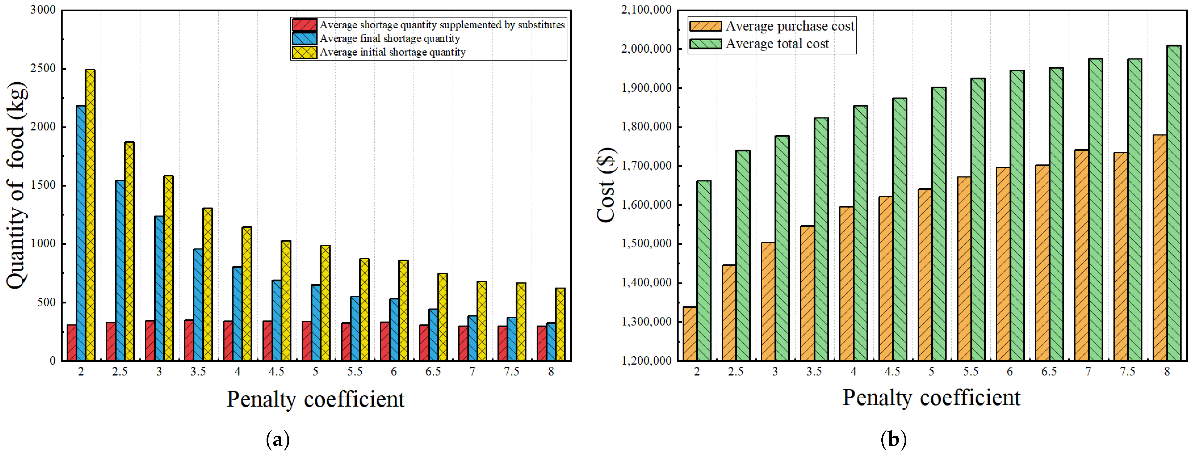
As shown in Table 8 and depicted in Figure 2a, as the penalty coefficient increases from 2.0 to 8.0, all shortage-related quantities demonstrate a consistent declining trend. The initial shortage quantity decreases from 2490.08 kg to 622.23 kg (a 75.0% reduction), while the final shortage quantity drops from 2183.58 kg to 323.54 kg (an 85.2% reduction). Concurrently, the substitution rate shows a steady increase from 12.3% to 48.0%, indicating enhanced utilization of the substitution mechanism under higher penalty pressures.

Figure 2. Impact of shortage penalty coefficient on key factors.(a) Shortage quantities. (b) Cost components.

The cost dynamics illustrated in Figure 2b reveal a contrasting pattern. As the penalty coefficient rises, both the purchase cost and total cost exhibit continuous growth. The total cost increases from 1,662,081.76 to 2,009,200.58 (a 20.9% increase), reflecting the economic trade-off between shortage mitigation and cost efficiency. This correlation demonstrates that higher penalty coefficients drive the model to adopt more conservative procurement strategies, significantly reducing shortage risks at the expense of elevated operational costs.

The analysis reveals three distinct phases in the model’s response to increasing penalty coefficients: (1) In the low penalty range (2.0–4.0), substantial shortage reduction is achieved with relatively moderate cost increases, indicating high marginal returns; (2) in the medium range (4.0–6.0), diminishing returns become apparent as additional cost increments yield progressively smaller shortage improvements; (3) in the high range (6.0–8.0), further shortage reduction requires disproportionately high cost increases, highlighting the optimal operational range for practical decision making where cost-effectiveness begins to decline significantly.

4.3.4. Sensitivity Analysis on Different Salvage Value Coefficient $s_i$

The salvage value coefficient $s_i$ plays a crucial role in determining procurement strategy. When $s_i$ is negative, it represents disposal costs for leftover food, discouraging over-purchasing as the food becomes unusable after the voyage. Conversely, a positive $s_i$ indicates residual value, encouraging larger procurement quantities.

As shown in Table 9, increasing $s_i$ leads to higher procurement quantities, resulting in increased purchase costs but reduced shortage costs. The higher procurement levels also provide more available food for substitution, leading to increased substitution costs. This trade-off reflects the fundamental balance between procurement strategy and shortage management.

Table 9. Decision results under salvage value $s_i$.

${\mathit{s}}_{\mathit{i}}$	Purchase Cost	Purchase Cost Proportion (%)	Shortage Cost	Shortage Cost Proportion (%)	Substitution Cost	Salvage Value
$-0.3$	1,344,943.95	91.40	114,414.84	7.78	865.96	$-11,311.58$
$-0.2$	1,349,126.11	92.09	106,685.48	7.28	928.78	$-8220.57$
$-0.1$	1,356,786.32	92.80	99,875.77	6.83	949.55	$-4463.27$
0.1	1,373,900.92	94.43	85,280.72	5.86	1079.09	5353.01
0.2	1,378,209.37	95.36	77,725.26	5.38	1079.56	11,721.60
0.3	1,388,411.46	96.38	70,149.59	4.87	1088.94	19,060.90

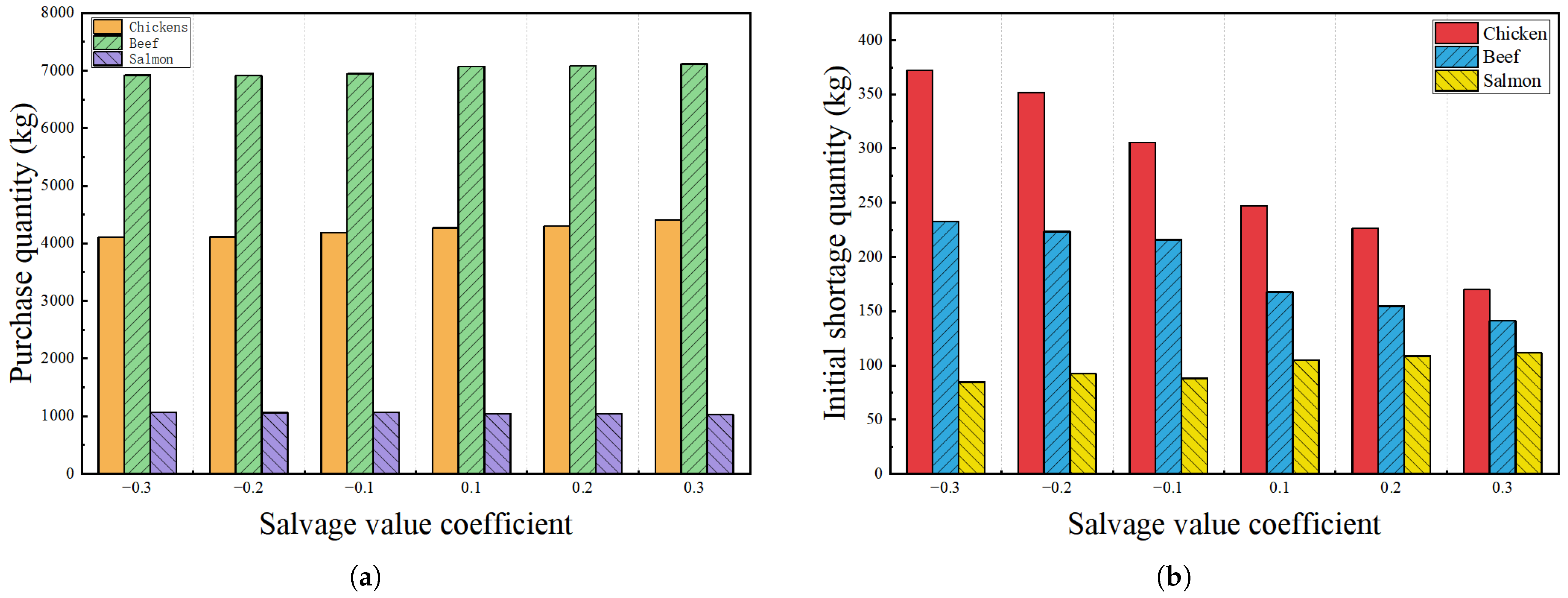
Examining the three key meat products reveals interesting patterns. Figure 3a demonstrates that both chicken and beef procurement quantities increase with higher $s_i$, while salmon purchases show a slight decrease. This occurs because salmon’s relatively lower demand can be effectively supplemented by other meat products through substitution. The increased procurement of chicken and beef provides sufficient buffer to cover potential salmon shortages.

Figure 3. Impact of salvage value coefficient on key factors. (a) Purchase quantities. (b) Initial shortage quantities.

The benefits of higher $s_i$ are clearly visible in Figure 3b, where initial shortage quantities show significant reduction across all products. This improvement is further quantified in Table 10 for the key meat products. As $s_i$ increases from $-0.3$ to $0.3$, chicken shortages demonstrate a significant reduction from 268.11 to 102.87 units, while beef shortages show a substantial decline from 232.45 to 140.98 units. Interestingly, salmon shortages remain relatively stable throughout the salvage value range, fluctuating between 43.23 and 48.93 units with no clear trend. The results demonstrate that positive salvage values encourage more strategic procurement planning, particularly benefiting products with higher demand variability.

Table 10. Final shortage for key meat products.

Salvage Value Coefficient	Chicken	Beef	Salmon
$-0.3$	268.11	232.45	46.60
$-0.2$	248.35	223.18	48.51
$-0.1$	209.04	215.67	43.23
0.1	162.57	167.66	48.93
0.2	144.92	154.53	48.66
0.3	102.87	140.98	48.80

The results suggest that cruise operators can strategically adjust their salvage value assumptions based on their operational capabilities and food preservation technologies. Higher salvage values encourage more aggressive procurement strategies, which significantly reduce shortages but require careful management of substitution relationships and storage constraints.

4.3.5. Sensitivity Analysis on Substitute Cost Coefficient $d_{ij}$

The results in Table 11 demonstrate how changes in the substitute cost coefficient $d_{ij}$ influence the provisioning system. As $d_{ij}$ increases, the total substitution cost shows a direct upward trend, while the total shortage cost generally decreases. To better understand this relationship, we focus on three main meat products: beef, salmon, and chicken.

Table 11. Decision results under different substitute cost coefficient $d_{ij}$.

Substitute Cost Coefficient	Purchase Cost	Shortage Cost	Substitution Cost	Salvage Value	Total Cost
0.1	1,354,042.93	101,915.75	925.23	$-4390.16$	1,461,274.07
0.2	1,357,367.44	100,668.91	1867.38	$-4429.70$	1,464,333.44
0.3	1,353,940.29	99,636.84	2476.22	$-4399.00$	1,460,452.36
0.4	1,355,762.07	102,173.49	3117.38	$-4392.40$	1,465,445.34
0.5	1,354,269.72	103,916.41	4178.67	$-4437.47$	1,466,802.27
0.6	1,356,744.51	94,305.09	5693.65	$-4578.71$	1,461,321.96
0.7	1,353,703.05	97,497.01	6335.24	$-4545.29$	1,462,080.59
0.8	1,352,952.26	95,324.02	8097.53	$-4625.46$	1,460,999.28

The economic feasibility of any substitution is determined by the condition $p_j·q_{ij}+d_{ij}>p_i$. An increase in $d_{ij}$ directly influences the satisfaction of this inequality. As $d_{ij}$ rises, the left-hand side of the inequality increases, making it easier to satisfy the condition. Consequently, more substitution relationships that are previously economically infeasible may become viable.

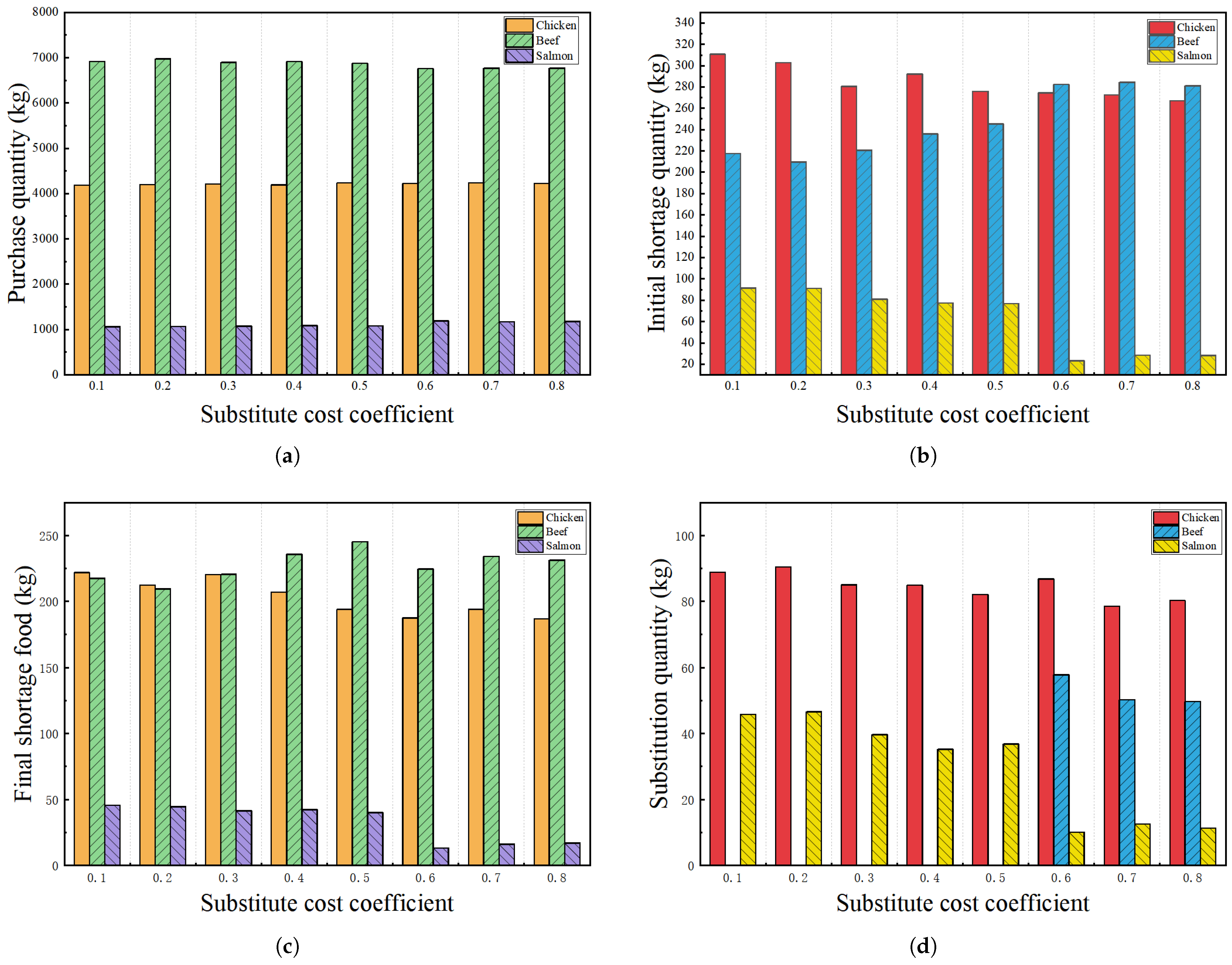
Specifically, when $d_{ij}$ increases to the threshold of 0.6, the condition $p_j·q_{ij}+d_{ij}>p_i$ is met for the case where salmon substitutes for beef. This activates a new substitution pathway from salmon to beef, as a substitution from beef to salmon is already feasible under lower $d_{ij}$ values. This new pathway establishes a two-way substitution relationship between beef and salmon, enhancing the flexibility within the provisioning system.

This structural change significantly impacts procurement patterns. Figure 4a illustrates that when $d_{ij}\ge 0.6$, beef purchases decline while salmon purchases increase. For $d_{ij}<0.6$, the system relies on beef as a buffer for potential shortages of both salmon and chicken. However, as $d_{ij}$ rises, this strategy becomes less economically viable, leading to increased initial beef shortages, as shown in Figure 4b.

Figure 4. Impact of the substitute cost coefficient on key factors. (a) Purchase quantities. (b) Initial shortage quantities. (c) Final shortage quantities. (d) Substitution quantities.

The activation of two-way substitution changes procurement strategies. Beef purchases decrease as a result. Salmon purchases increase correspondingly. This leads to persistently high beef shortages. Meanwhile, salmon shortages drop significantly, as shown in Figure 4b. This pattern offers a key managerial insight: two-way substitution makes purchasing more rational. The system no longer relies heavily on substitution as a primary solution. Instead, it prioritizes sufficient procurement of each main food category. Substitution only serves as a backup for unexpected shortages. This approach establishes a more robust and cost-effective provisioning system.

From a managerial perspective, establishing appropriate substitution costs to enable two-way substitution relationships is crucial for optimizing procurement and shortage management strategies. Such bidirectional substitution mechanisms create more flexible and resilient provisioning systems that can better adapt to demand fluctuations. More importantly, two-way substitution relationships ensure more rational procurement decisions by preventing unreasonable one-way substitution patterns in the optimization results. This approach guides managers to make balanced procurement plans for various food categories during the decision-making process, rather than relying excessively on substituting one specific food item for others. Managers should carefully calibrate substitution costs to activate economically feasible two-way relationships, thereby achieving a more balanced and practical provisioning strategy that maintains both operational efficiency and service quality.

Despite the observed changes, the substitution mechanism effectively controls overall shortages, as demonstrated in Figure 4c,d. For products experiencing persistent shortages such as chicken and beef, additional adjustments to their shortage penalty coefficients $p_i$ could provide further improvements in shortage control performance.

4.3.6. Sensitivity Analysis of Service Level Coefficient ${\lambda }_i$

The impact of service level coefficients on the provisioning system is analyzed by varying ${\lambda }_i$ from 0.75 to 0.95, where ${\lambda }_i$ represents the minimum proportion of demand that must be fulfilled by the original product. As shown in Table 12, the substitution quantity demonstrates an increasing trend as the service level coefficient decreases, rising from 191.20 kg to 338.76 kg when ${\lambda }_i$ decreases from 0.95 to 0.75. This pattern is reflected in the substitution rate, which is calculated as the ratio of substitution quantity to initial shortage quantity, i.e., $\mathrm{Substitution}\mathrm{Rate}={\displaystyle \frac{\mathrm{Total}\mathrm{Substitution}\mathrm{Quantity}}{\mathrm{Initial}\mathrm{Shortage}\mathrm{Quantity}}}\times 100\%$. The substitution rate increases from 9.5% to 15.6% over the tested range, with the highest value of 16.1% achieved at ${\lambda }_i=0.80$, indicating that lower service level constraints enable greater utilization of the substitution mechanism.

Table 12. Decision results under different service level coefficients ${\lambda }_i$.

Service Level Coefficient	Initial Shortage Quantity (kg)	Final Shortage Quantity (kg)	Substitution Quantity (kg)	Substitution Rate (%)
0.95	2003.73	1812.53	191.20	9.5
0.90	2103.52	1828.32	275.20	13.1
0.85	2090.99	1761.07	329.92	15.8
0.80	2132.21	1788.35	343.86	16.1
0.75	2165.67	1826.91	338.76	15.6

Analysis of shortage patterns reveals that both initial and final shortage quantities vary with service level changes. Initial shortages increase from 2003.73 kg to 2165.67 kg as the service level coefficient decreases from 0.95 to 0.75, while final shortages show a similar increasing pattern from 1761.07 kg to 1826.91 kg. This observation indicates that while the service level constraint directly limits the maximum allowable substitution proportion to $(1-{\lambda }_i)$, the actual substitution utilization is predominantly determined by the optimization model based on economic feasibility and resource availability. The variation in shortage quantities across different service levels demonstrates the trade-off between service quality requirements and shortage management effectiveness.

The cost analysis in Table 13 reveals that the total cost decreases from 1,469,343.53 to 1,460,076.78 as the service level coefficient decreases from 0.95 to 0.75, representing a 0.6% overall cost reduction. This improvement is primarily driven by the decreasing shortage cost, which drops from 105,953.05 to 102,306.58, despite a moderate increase in substitution cost from 414.06 to 988.63. The purchase cost remains relatively stable across different service levels, fluctuating between 1,352,452.37 and 1,358,386.85, demonstrating that procurement decisions are largely independent of service level parameter settings. These results collectively suggest that implementing moderately lower service level coefficients enhances system flexibility and cost efficiency without compromising operational stability. The optimal balance between substitution effectiveness and economic performance is achieved at ${\lambda }_i=0.80$, where the system maintains adequate service quality while minimizing total operational costs.

Table 13. Shortage quantities under different service level coefficients ${\lambda }_i$.

Service Level Coefficient	Purchase Cost	Shortage Cost	Substitution Cost	Salvage Value	Total Cost
0.95	1,358,386.85	105,953.05	414.06	−4589.57	1,469,343.53
0.90	1,355,774.57	103,024.11	693.42	−4357.47	1,463,849.57
0.85	1,358,232.36	100,862.85	917.17	−4471.64	1,464,484.02
0.80	1,354,790.34	100,022.43	957.14	−4402.20	1,460,172.11
0.75	1,352,452.37	102,306.58	988.63	−4329.20	1,460,076.78

5. Practical Implications

The implementation of the two-stage stochastic optimization framework offers substantial practical value for cruise ship operators in managing food provisioning operations. This research provides actionable insights that can directly enhance operational decision making, cost management, and risk mitigation strategies.

For operational decision support, the model serves as an effective tool for provisioning managers, enabling data-driven procurement planning under uncertainty. Cruise operators can utilize this framework to move beyond traditional deterministic planning methods that often lead to either costly overstocking or service-disrupting shortages. The scenario-based approach provides specific guidance on optimal purchase quantities for each food category while considering storage constraints and substitution possibilities.

Regarding cost management, the sensitivity analyses reveal crucial strategic insights. The strong correlation between procurement prices and total costs underscores the importance of securing stable supply contracts and implementing cost-effective sourcing strategies. The identification of optimal service level coefficients (${\lambda }_i=0.80$) enables operators to balance substitution flexibility with cost control, achieving approximately 0.6% cost reduction compared to restrictive substitution policies. Furthermore, the salvage value analysis demonstrates how strategic over-procurement with positive salvage assumptions can effectively control shortage risks while maintaining cost efficiency.

In terms of risk mitigation, the framework provides robust mechanisms for handling demand uncertainty. The substitution protocols establish resilient backup systems that can compensate for 12–17% of shortage volumes during demand fluctuations. The penalty coefficient analysis offers guidance on setting appropriate shortage penalties that balance service quality objectives with cost considerations. Additionally, the storage capacity constraints ensure that provisioning plans remain feasible within the physical limitations of cruise ship facilities.

The practical implementation of this optimization framework can lead to more resilient provisioning systems, reduced operational costs, and enhanced passenger satisfaction through improved dining experience consistency. Cruise operators can adapt these findings to develop more sophisticated inventory management systems that proactively address the unique challenges of maritime food logistics.

6. Conclusions

Effective food provisioning is a fundamental requirement for cruise ship operations. This process directly determines operational profitability and passenger satisfaction levels. Modern cruise ships function as large floating resorts. They must provide consistent dining experiences for thousands of people. These voyages often extend for weeks without port calls. The scale of consumption creates significant logistical challenges. Demand uncertainty remains a persistent issue in planning. Traditional planning methods based on average demand often prove inadequate. They frequently lead to either overstocking or problematic shortages. This operational reality underscores the urgent need for advanced decision-support systems. Our research directly addresses this critical industry need.

We present a two-stage stochastic optimization framework. This model specifically addresses the unique challenges of cruise food provisioning. The first-stage decisions involve procurement planning before voyage departure. These decisions must account for specialized storage constraints. The ship has freezer, refrigerator, and ambient storage compartments. Each has distinct capacity limitations and compatibility requirements. The second-stage decisions occur after observing actual demand. They determine optimal substitution strategies to mitigate shortages. Our model incorporates realistic substitution relationships between food items. Each substitution carries specific nutritional and cost parameters. To solve this complex stochastic program, we employ SAA. This method uses multiple randomly generated demand scenarios. We implement comprehensive statistical validation procedures. These procedures establish reliable lower bounds. The lower bounds are derived by solving multiple independent SAA problems. These procedures also establish reliable upper bounds. The upper bounds are obtained by evaluating candidate solutions against large reference samples. They also calculate precise optimality gaps. These gaps provide solution quality assurance.

Our numerical experiments employ authentic cruise operational data encompassing fourteen major food categories. The convergence analysis reveals that a scenario size of 80 achieves an optimal balance between solution quality and computational efficiency, yielding an optimality gap of 0.78% while maintaining practical computational requirements for operational planning. The comprehensive sensitivity analysis provides valuable managerial insights across multiple dimensions. First, increasing demand variance leads to elevated total costs, while food price fluctuations demonstrate significant impact on overall expenditure. Second, the shortage penalty coefficient substantially influences procurement strategy, with higher coefficients driving increased purchase quantities and consequently reducing final shortages by up to 85.2% when the coefficient rises from 2.0 to 8.0. Third, appropriate substitution cost calibration facilitates the establishment of two-way substitution relationships, such as between beef and salmon, thereby creating more resilient and flexible provisioning systems. Fourth, salvage value assumptions significantly affect procurement behavior, where positive salvage values encourage strategic over-procurement, effectively controlling shortage risks while maintaining cost efficiency. Furthermore, the service level analysis demonstrates that moderate service level coefficients (around ${\lambda }_i=0.80$) achieve an optimal balance between substitution flexibility and cost control. Higher service levels enhance system responsiveness to shortages through increased substitution capacity, while lower levels maintain tighter control over substitution costs, with the optimal configuration reducing total costs by approximately 0.6% compared to the most restrictive service level setting.

Future research should pursue several promising directions.

• Enhanced demand modeling: Detailed passenger information should be incorporated, including demographics and historical consumption patterns. Correlation analysis between different food items should be conducted to improve forecasting accuracy. Menu engineering principles could also be applied to refine demand projections.
• Algorithmic improvements: Advanced decomposition methods, such as Benders decomposition, should be developed to handle larger problem instances more efficiently. These methods would substantially improve computational performance.
• Machine learning integration: Predictive analytics should be employed to optimize scenario generation processes. These techniques can generate more accurate demand scenarios, thereby enhancing the stochastic optimization framework.

References

1. Yang, Y.; Zhang, S.; Wang, S. Integrated cruise fleet deployment and itinerary scheduling problem: An enhanced Benders decomposition approach. Transp. Res. Part B Methodol. 2025, 201, 103321. [Google Scholar] [CrossRef]
2. Brida, J.G.; Chiappa, G.D.; Meleddu, M.; Pulina, M. A comparison of residents’ perceptions in two cruise ports in the Mediterranean Sea. Int. J. Tour. Res. 2014, 16, 180–190. [Google Scholar] [CrossRef]
3. Huang, L.; Tan, Y.; Yue, X. Optimizing route and speed under the sulfur emission control areas for a cruise liner: A new strategy considering route competitiveness and low carbon. Mathematics 2024, 12, 1847. [Google Scholar] [CrossRef]
4. Hung, K.; Wang, S.; Denizci, G.B.; Liu, Z. An overview of cruise tourism research through comparison of cruise studies published in English and Chinese. Int. J. Hosp. Manag. 2019, 77, 207–216. [Google Scholar] [CrossRef]
5. Sun, X.; Kwortnik, R.; Gauri, D.K. Exploring behavioral differences between new and repeat cruisers to a cruise brand. Int. J. Hosp. Manag. 2018, 71, 132–140. [Google Scholar] [CrossRef]
6. Vega-Muñoz, A.; Arjona-Fuentes, J.M.; Ariza-Montes, A.; Han, H.; Law, R. In search of a research front in cruise tourism studies. Int. J. Hosp. Manag. 2020, 85, 102353. [Google Scholar] [CrossRef]
7. Papathanassis, A. Cruise tourism research: A horizon 2050 paper. Tour. Rev. 2025, 80, 165–180. [Google Scholar] [CrossRef]
8. Véronneau, S.; Roy, J. Global service supply chains: An empirical study of current practices and challenges of a cruise line corporation. Tour. Manag. 2009, 30, 128–139. [Google Scholar] [CrossRef]
9. Li, N.; Wang, J. Food waste of Chinese cruise passengers. J. Sustain. Tour. 2020, 28, 1825–1840. [Google Scholar] [CrossRef]
10. Compact Histories. The History of Passenger Cruises. Available online: https://compacthistories.com/history/the-history-of-passenger-cruises (accessed on 30 September 2025).
11. Rodrigue, J.P.; Wang, G.W.Y. Cruise ship supply chains and the impacts of disruptions: The case of the Caribbean. Res. Transp. Bus. Manag. 2022, 45, 100551. [Google Scholar] [CrossRef]
12. My Cruise Ship Info. Golden Harvest Shipping Service Co., Ltd. (Shanghai). Available online: https://www.mycruiseship.info/ship-suppliers/details/golden-harvest-shipping-service-co-ltd-shanghai (accessed on 30 September 2025).
13. Gu, B.; Liu, J.; Chen, J. Scenario-based strategies evaluation for maritime supply chain resilience. Transp. Res. Part D Transp. Environ. 2023, 124, 103948. [Google Scholar] [CrossRef]
14. Wang, K.; Wang, S.; Zhen, L.; Qu, X. Cruise ship operations planning and research opportunities. Marit. Bus. Rev. 2016, 1, 133–148. [Google Scholar] [CrossRef]
15. Wang, C.; Peng, Z.; Xu, W. Robust bi-level optimization for maritime emergency materials distribution in uncertain decision-making environments. Mathematics 2023, 11, 4140. [Google Scholar] [CrossRef]
16. Upadhaya, A.; Telle, J.S.; Schlüters, S.; Saber, M.; von Maydell, K. A robust approach to extend deterministic models for the quantification of uncertainty and comprehensive evaluation of probabilistic forecasting. Int. J. Energy Res. 2025, 2025, 4460462. [Google Scholar] [CrossRef]
17. Tao, Y.; Yang, Y.; Wang, S. A data-driven semi-relaxed MIP model for decision-making in maritime transportation. Mathematics 2025, 13, 2946. [Google Scholar] [CrossRef]
18. Erkoc, M.; Iakovou, E.T.; Spaulding, A.E. Multi-stage onboard inventory management policies for food and beverage items in cruise liner operations. J. Food Eng. 2005, 70, 269–279. [Google Scholar] [CrossRef]
19. Zhou, J.; Chen, S.L.; Shi, W. Identifying risks in the cruise supply chain: An empirical study in Shanghai, China. Transp. Res. Rec. 2023, 2677, 1706–1720. [Google Scholar] [CrossRef]
20. Meng, S.; Wu, X. Risk analysis of cruise ship supply chain based on the set pair analysis-Markov chain model. Ocean Coast. Manag. 2023, 245, 106855. [Google Scholar] [CrossRef]
21. Pasternack, B.A.; Drezner, Z. Optimal inventory policies for substitutable commodities with stochastic demand. Nav. Res. Logist. 1991, 38, 221–240. [Google Scholar] [CrossRef]
22. Nagarajan, M.; Rajagopalan, S. Inventory models for substitutable products: Optimal policies and heuristics. Manag. Sci. 2008, 54, 1453–1466. [Google Scholar] [CrossRef]
23. Ahiska, S.S.; Kurtul, E. Modeling and analysis of a product substitution strategy for a stochastic manufacturing/remanufacturing system. Comput. Ind. Eng. 2014, 72, 1–11. [Google Scholar] [CrossRef]
24. Rao, U.S.; Swaminathan, J.M.; Zhang, J. Multi-product inventory planning with downward substitution, stochastic demand and setup costs. IIE Trans. 2004, 36, 59–71. [Google Scholar] [CrossRef]
25. Kim, S.W.; Bell, P.C. Stochastic optimization models with substitution as a result of price differences and stockouts. Int. Trans. Oper. Res. 2019, 26, 2129–2151. [Google Scholar] [CrossRef]
26. Biehn, N. A cruise ship is not a floating hotel. J. Revenue Pricing Manag. 2006, 5, 135–142. [Google Scholar] [CrossRef]
27. Castillo-Manzano, J.I.; Castro-Nuño, M.; Pozo-Barajas, R. Foodies on board! Exploring cruiser satisfaction with the culinary experience. Int. J. Gastron. Food Sci. 2025, 41, 101238. [Google Scholar] [CrossRef]
28. Suárez-de Vivero, J.L.; Rodríguez Mateos, J.C.; Florido del Corral, D.; Barragán, M.J.; Calado, H.; Kjellevold, M.; Miasik, E.J. Food security and maritime security: A new challenge for the European Union’s ocean policy. Mar. Policy 2019, 108, 103640. [Google Scholar] [CrossRef]
29. Bo, A.; Wang, C.J.; Gou, Y.C. Seasonality and spatial patterns of cruise ports from a shipping perspective: A case study of the Mediterranean. J. Chin. Ecotour. 2024, 14, 816–833. [Google Scholar]
30. Fernández-Morales, A.; Cisneros-Martínez, J.D.; McCabe, S. Seasonal concentration of tourism demand: Decomposition analysis and marketing implications. Tour. Manag. 2016, 56, 172–190. [Google Scholar] [CrossRef]
31. Diabat, A.; Govindan, K.; Panicker, V.V. Supply chain risk management and its mitigation in a food industry. Int. J. Prod. Res. 2012, 50, 3039–3050. [Google Scholar] [CrossRef]
32. Zhang, J.; Ma, P.; Zhong, W.; Meng, C. Projection-based techniques for high-dimensional optimal transport problems. Wiley Interdiscip. Rev. Comput. Stat. 2023, 15, e1587. [Google Scholar] [CrossRef]
33. Zhang, S.; Sridharan, M. A survey of knowledge-based sequential decision-making under uncertainty. AI Mag. 2022, 43, 249–266. [Google Scholar] [CrossRef]
34. Sun, X.; Jiao, Y.; Tian, P. Marketing research and revenue optimization for the cruise industry: A concise review. Int. J. Hosp. Manag. 2011, 30, 746–755. [Google Scholar] [CrossRef]
35. Zhang, J. Stochastic Programming Approaches to Multi-Product Inventory Management Problems with Substitution. Ph.D. Thesis, Virginia Polytechnic Institute and State University, Blacksburg, VA, USA, 2019. Available online: https://vtechworks.lib.vt.edu/bitstream/handle/10919/95209/Zhang_J_D_2019.pdf (accessed on 30 September 2025).
36. Zhang, J.; Xie, W.; Sarin, S. Multiproduct newsvendor problem with customer-driven demand substitution: A stochastic integer program perspective. INFORMS J. Comput. 2021, 33, 1229–1244. [Google Scholar] [CrossRef]
37. Lau, Y.-Y.; Yip, T.L. The procurement of food on board liner ships: The role of the International Labour Organization. J. Shipp. Trade 2017, 2, 6. [Google Scholar] [CrossRef]
38. Stefanova, M. Sustainable Logistics Services of Food Provisions on Merchant Ships; MDPI: Basel, Switzerland, 2025; Available online: https://www.mdpi.com/books/monograph/11185-sustainable-logistics-services-of-food-provisions-on-merchant-ships (accessed on 30 September 2025).
39. Koren, M.; Perlman, Y.; Shnaiderman, M. Inventory management for stockout-based substitutable products under centralised and competitive settings. Int. J. Prod. Res. 2024, 62, 3176–3192. [Google Scholar] [CrossRef]
40. Ghorashi Khalilabadi, S.M.; Zegordi, S.H.; Nikbakhsh, E. A multi-stage stochastic programming approach for supply chain risk mitigation via product substitution. Comput. Ind. Eng. 2020, 149, 106786. [Google Scholar] [CrossRef]
41. Glasserman, P.; Yao, D.D. Some guidelines and guarantees for common random numbers. Manag. Sci. 1992, 38, 884–908. [Google Scholar] [CrossRef]
42. Wright, R.D.; Ramsay, T.E. On the effectiveness of common random numbers. Manag. Sci. 1979, 25, 649–656. [Google Scholar] [CrossRef]
43. Feeding the Largest Cruise Ships in the World. Available online: https://edition.cnn.com/travel/article/cruise-ships-food-supplies (accessed on 30 September 2025).
44. What It Takes to Stock a Cruise Ship: 10,680 Hot Dogs and a Boatload of Wine. Available online: https://mashable.com/article/cruise-ship-food (accessed on 30 September 2025).
45. United States Department of Agriculture (USDA). Available online: https://www.usda.gov/ (accessed on 30 September 2025).
46. Ministry of Agriculture and Rural Affairs of the People’s Republic of China (MARA). Available online: https://www.moa.gov.cn/ (accessed on 30 September 2025).
47. Baidu Health. Available online: https://jiankang.baidu.com/ (accessed on 30 September 2025).
48. Petruzzi, N.C.; Dada, M. Pricing and the newsvendor problem: A review with extensions. Oper. Res. 1999, 47, 183–194. [Google Scholar] [CrossRef]
49. Patriarca, R.; Di Gravio, G.D.; Costantino, F.; Tronci, M. EOQ inventory model for perishable products under uncertainty. Prod. Eng. 2020, 14, 601–612. [Google Scholar] [CrossRef]
50. Mishra, V.K. Optimal ordering quantities for substitutable deteriorating items under joint replenishment with cost of substitution. J. Ind. Prod. Eng. 2017, 34, 233–245. [Google Scholar] [CrossRef]
51. Deniz, B.; Chan, F.T.S.; Caplice, C.; Johnson, M.E. Managing perishables with substitution: Inventory issuance decisions for perishables. Manuf. Serv. Oper. Manag. 2010, 12, 296–315. [Google Scholar] [CrossRef]
52. How Do Cruise Ships Stock Up on Food (Both in Summer and Winter)? Available online: https://www.cookist.com/how-do-cruise-ships-stock-up-on-food-both-in-summer-and-winter/ (accessed on 30 September 2025).
53. How Is Food Stored on a Cruise Ship? Available online: https://luxurytraveldiva.com/how-is-food-stored-on-a-cruise-ship/ (accessed on 30 September 2025).
54. Strijbosch, L.W.G.; Moors, J.J.A. Modified normal demand distributions in (R, S) inventory models. Int. J. Prod. Econ. 2003, 84, 61–72. [Google Scholar] [CrossRef]
55. Saxena, V.; Singh, J.; Kumari, N. An analytical approach to inventory management under truncated normal demand distribution. Libr. Prog. Int. 2024, 44, 14807–14818. [Google Scholar]
56. Foster, F.G.; Rosenhead, J.V.; Siskind, V. The effect of the demand distribution in inventory models combining holding, stockout and re-order costs. J. R. Stat. Soc. Ser. B Methodol. 1971, 33, 312–325. [Google Scholar] [CrossRef]
57. Bertsimas, D.; Gupta, V.; Kallus, N. Robust sample average approximation. Math. Program. 2018, 171, 217–282. [Google Scholar] [CrossRef]
58. Anderson, E.; Philpott, A. Improving sample average approximation using distributional robustness. INFORMS J. Optim. 2022, 4, 90–124. [Google Scholar] [CrossRef]
Disclaimer/Publisher’s Note: The statements, opinions and data contained in all publications are solely those of the individual author(s) and contributor(s) and not of MDPI and/or the editor(s). MDPI and/or the editor(s) disclaim responsibility for any injury to people or property resulting from any ideas, methods, instructions or products referred to in the content.
Article Metrics
Citations
Article Access Statistics
Multiple requests from the same IP address are counted as one view.