Nonlinear Optical Characteristics of Copper Oxide Thin Films Interpreted Through Soliton Solutions of the Convective–Diffusive Cahn–Hilliard Equation

Abstract

This study investigates the convective–diffusive Cahn–Hilliard equation, a nonlinear model which is used in real-world applications to phase separation and material pattern formation. Using the modified Sardar sub-problem technique, which is an extension of the Sardar sub-equation approach, we derive multiple classes of exact soliton solutions, including bright, dark, kink, and periodic forms. The parametric behaviors of these solutions are examined and visualized through analytical plots generated in Mathematica and Maple. Furthermore, UV–Vis spectrophotometry is employed to examine the optical response of copper oxide (CuO) thin films. The films exhibited a sharp absorption edge around 380–410 nm and an optical band gap of approximately 2.3 eV, confirming their semiconducting nature. The experimentally observed periodic transmission characteristics are linked with the theoretical soliton profiles predicted by the model. Overall, the proposed analytical and experimental framework establishes a clear connection between nonlinear wave theory and thin-film optical characterization, providing new insights into soliton transformation phenomena in complex material systems.

1. Introduction

In this section, the background summarizes prior research relevant to the model being examined. It highlights the gaps in the current literature, defines the main contributions of the study, and outlines the layout of the paper.

1.1. Background Study and Mathematical Model

The Cahn–Hilliard equation is a fundamental nonlinear partial differential equation used to describe phase separation, spinodal decomposition, and pattern formation in multi-component materials. For a binary alloy or thin-film mixture, the state of the system at time t is represented by the concentration fields ${\mathcal{A}}_{\mathrm{Cr}}$ and ${\mathcal{A}}_{\mathrm{x}}$ corresponding to the atomic fractions of species X and $Cr$. To examine the soliton solutions to the convective–diffusive Cahn–Hilliard model described below [1,2], the following system is considered:

$$\begin{array}{c}\hfill \left\{\begin{array}{cc}{\left({\mathcal{A}}_{\mathrm{Cr}}\right)}_t={\mathcal{P}}_{\mathrm{Cr}}{\left({\mathcal{Q}}_{{\mathcal{A}}_{\mathrm{Cr}}}-{\mathcal{S}}_{\mathrm{Cr}}{\left({\mathcal{A}}_{\mathrm{Cr}}\right)}_{xx}-{\mathcal{R}}_{\mathrm{Cr}X}{\left({\mathcal{A}}_x\right)}_{xx}\right)}_{xx},\hfill & \hfill \\ {\left({\mathcal{A}}_x\right)}_t={\mathcal{P}}_x{\left({\mathcal{Q}}_{{\mathcal{A}}_x}-{\mathcal{S}}_x{\left({\mathcal{A}}_{\mathrm{Cr}}\right)}_{xx}-{\mathcal{R}}_x{\left({\mathcal{A}}_x\right)}_{xx}\right)}_{xx}.\hfill & \hfill \end{array}\right.\end{array}$$

(1)

In system (1), the attractive areas of features X and $\mathrm{Cr}$ are represented by ${\mathcal{A}}_x(x,t)$ as well as ${\mathcal{A}}_{\mathrm{Cr}}(x,t)$, by using Maple software, respectively [3,4].

$$\begin{array}{c}\hfill \left\{\begin{array}{cc}{\left({\mathcal{A}}_{\mathrm{Cr}}\right)}_t={\mathcal{P}}_{\mathrm{Cr}}\left[\right({\mathcal{Q}}_{{\mathcal{A}}_{\mathrm{Cr}}^2}{\left({\mathcal{A}}_{\mathrm{Cr}}\right)}_{xx}+{\mathcal{Q}}_{{\mathcal{A}}_{\mathrm{Cr}{\mathcal{A}}_x}}{\left({\mathcal{A}}_x\right)}_{xx}+2{\mathcal{Q}}_{{\mathcal{A}}_{\mathrm{Cr}}^2{\mathcal{A}}_x}{\left({\mathcal{N}}_{\mathrm{Cr}}\right)}_x{\left({\mathcal{A}}_x\right)}_x,\hfill & \hfill \\ +{\mathcal{Q}}_{{\mathcal{A}}_{\mathrm{Cr}}^3}{\left({\left({\mathcal{A}}_{\mathrm{Cr}}\right)}_x\right)}^2+{\mathcal{Q}}_{{\mathcal{A}}_{\mathrm{Cr}}{\mathcal{A}}_x^2}{\left({\left({\mathcal{A}}_x\right)}_x\right)}^2-{\mathbf{S}}_{\mathrm{Cr}}{\left({\mathcal{N}}_{\mathrm{Cr}}\right)}_{xxx}-{\mathcal{R}}_{\mathrm{Cr}X}{\left({\mathcal{A}}_x\right)}_{xxxx}\left)\right]\hfill & \hfill \\ {\left({\mathcal{A}}_x\right)}_t={\mathcal{P}}_x\left[\right({\mathcal{Q}}_{{\mathcal{A}}_{\mathrm{Cr}}^2{\mathcal{A}}_x}{\left({\mathcal{A}}_{\mathrm{Cr}}\right)}_{xx}+{\mathcal{Q}}_{{\mathcal{A}}_x^2}{\left({\mathcal{A}}_x\right)}_{xx}+2{\mathcal{Q}}_{{\mathcal{A}}_{\mathrm{Cr}}^2{\mathcal{A}}_x^2}{\left({\mathcal{N}}_{\mathrm{Cr}}\right)}_x{\left({\mathcal{A}}_x\right)}_x,\hfill & \hfill \\ +{\mathcal{Q}}_{{\mathcal{A}}_{\mathrm{Cr}}^2{\mathcal{A}}_x}{\left({\left({\mathcal{A}}_{\mathrm{Cr}}\right)}_x\right)}^2+{\mathcal{Q}}_{{\mathcal{A}}_{\mathrm{Cr}}{\mathcal{A}}_x^3}{\left({\left({\mathcal{A}}_x\right)}_x\right)}^2-{\mathbf{R}}_{x\mathrm{Cr}}{\left({\mathcal{N}}_{\mathrm{Cr}}\right)}_{xxx}-{\mathcal{S}}_X{\left({\mathcal{A}}_x\right)}_{xxxx}\left)\right].\hfill \end{array}\right.\end{array}$$

(2)

The convective–diffusive Cahn–Hilliard equation is a generalized form of the classical Cahn–Hilliard model that incorporates both diffusive and convective transport effects. It is widely used to describe phase separation and mass redistribution in binary mixtures or thin films under external influences such as temperature gradients or deposition flux.

In the present model, two interacting features are considered, denoted by ${\mathcal{A}}_C(x,t)$ and ${\mathcal{A}}_X(x,t)$, which represent the concentration amplitudes of two coupled components within the system. The terms ${\mathcal{P}}_C$ and ${\mathcal{P}}_X$ denote diffusion coefficients or mobility parameters, while ${\mathcal{Q}}_{Ac},{\mathcal{Q}}_{AX}$ and ${\mathcal{S}}_C,{\mathcal{S}}_X,{\mathcal{R}}_C,{\mathcal{R}}_X$ are nonlinear interaction functions that account for convective and higher-order diffusion effects. The subscripts t and x represent partial derivatives with respect to time and space, respectively. The regular solution model allows for the expression of native free energy through an efficient mathematical connection that takes into consideration component interactions.

$$\begin{array}{c}\hfill \left\{\begin{array}{cc}\mathcal{Q}={\mathcal{Q}}^{*}\left(1-{\mathcal{A}}_{\mathrm{Cr}}-{\mathcal{A}}_x\right)+{\mathcal{Q}}^{**}{\mathcal{A}}_{\mathrm{Cr}}+{\mathcal{Q}}^{***}{\mathcal{A}}_x+{\mathbf{\Theta }}_{\mathrm{FeX}}{\mathcal{A}}_x\left(1-{\mathcal{A}}_{\mathrm{Cr}}-{\mathcal{A}}_x\right)+{\mathbf{\Theta }}_{\mathrm{FeCr}}{\mathcal{A}}_{\mathrm{Cr}}\hfill & \hfill \\ \left(1-{\mathcal{A}}_{\mathrm{Cr}}-{\mathcal{A}}_x\right)+{\mathbf{\Theta }}_{\mathrm{CrX}}{\mathcal{A}}_{Cr}{\mathcal{A}}_x+\mathcal{RT}[\left(1-{\mathcal{A}}_{\mathrm{Cr}}-{\mathcal{A}}_x\right)ln\left(1-{\mathcal{A}}_{\mathrm{Cr}}-{\mathcal{A}}_x\right)\hfill & \hfill \\ +{\mathcal{A}}_{\mathrm{Cr}}ln\left({\mathcal{A}}_{\mathrm{Cr}}\right)+{\mathcal{A}}_{x}ln\left({\mathcal{A}}_x\right)].\hfill & \hfill \end{array}\right.\end{array}$$

(3)

In this context, ${\mathcal{Q}}^{*},{\mathcal{Q}}^{**}$, and ${\mathcal{Q}}^{***}$ signify the energies corresponding to $Fe,Cr,$ and X, respectively. To evaluate the gradient energy and mobility in binary iron alloys such as $FeCr$ and $FeX$, we employ the convective–diffusive Cahn–Hilliard equation. These systems serve as representative examples for analyzing phase separation and transport mechanisms in metallic thin films. The parameters ${\mathbf{\Theta }}_{\mathrm{FeX}}$ and ${\mathbf{\Theta }}_{\mathrm{CrX}}$ serve as integration constants in the framework. In addition, $\mathcal{T}$ denotes absolute temperature and $\mathcal{R}$ is the gas constant, representing thermodynamic parameters. These factors work together to create the formulation shown in Equation (3), which embodies the linkages between the model’s energies and integration parameters while emphasizing its connection to both physical and thermodynamic systems. To simplify the nonlinear cdCH model and focus on the dominant transport mechanisms, a linearization or small-perturbation analysis is applied. By expanding the chemical potential around a stable reference concentration and retaining leading-order terms, the system reduces to Equation (3).

The evolution Equation (1) is obtained from the free-energy functional $F[{\mathcal{A}}_{Cr},{\mathcal{A}}_X]$ defined by the regular solution form in Equation (3). The chemical potentials for each component are defined by the functional derivative ${\mu }_i={\displaystyle \frac{\delta F}{\delta {\mathcal{A}}_i}}$. To isolate the leading transport behavior, the chemical potentials are expanded about a stable homogeneous reference state ${\mathcal{A}}_i={\mathcal{A}}_{i,0}+{\tilde{\mathcal{A}}}_i$, retaining only the leading-order terms in the perturbations ${\tilde{\mathcal{A}}}_i$ (small-perturbation/linearization assumption). Collecting diffusion, interfacial (fourth-order), and convective contributions then yields the algebraic equilibrium relations displayed in Equation (4). Under the stated assumptions and after appropriate non-dimensionalization and identification of transport coefficients, the model reduces to the scalar convective–diffusive Cahn–Hilliard form used throughout the analysis in Equation (5).

$$\begin{array}{c}\hfill \left\{\begin{array}{cc}{\mathcal{Q}}_{{\mathcal{A}}_{\mathrm{Cr}}^2}+2{\mathbf{\Theta }}_{\mathrm{FeCr}}-\mathcal{RT}\left[{\displaystyle \frac{1}{{\mathcal{A}}_{\mathrm{Cr}}}}+{\displaystyle \frac{1}{1-{\mathcal{A}}_{Cr}-{\mathcal{A}}_x}}\right]=0,\hfill & \hfill \\ {\mathcal{Q}}_{{\mathcal{A}}_x^2}+2{\mathbf{\Theta }}_{\mathrm{FeX}}-\mathcal{RT}\left[{\displaystyle \frac{1}{{\mathcal{A}}_x}}+{\displaystyle \frac{1}{1-{\mathcal{A}}_{Cr}-{\mathcal{A}}_x}}\right]=0,\hfill & \hfill \\ {\mathcal{Q}}_{{\mathcal{A}}_{\mathrm{Cr}}{\mathcal{A}}_x}-{\mathbf{\Theta }}_{\mathrm{CrX}}+{\mathbf{\Theta }}_{\mathrm{FeCr}}+{\mathbf{\Theta }}_{\mathrm{FeX}}-{\displaystyle \frac{\mathcal{RT}}{1-{\mathcal{A}}_{Cr}-{\mathcal{A}}_x}}=0.\hfill & \hfill \end{array}\right.\end{array}$$

(4)

These expressions describe the thermodynamic equilibrium condition arising from the free-energy minimization principle. To evaluate gradient energy and mobility in binary iron alloys like $\mathrm{Fe}-\mathrm{Cr}$ and $\mathrm{Fe}-\mathrm{X}$, use the convective–diffusive Cahn–Hilliard equation. These equations can subsequently be linearized, allowing for more extensive analysis and a simpler mathematical procedure for further investigation.

$$\begin{array}{c}\hfill {\left({\mathcal{A}}_{\iota }\right)}_t+{\mathrm{D}}_{\iota }{\left({\mathcal{A}}_{\iota }\right)}_{xx}+{\mathcal{P}}_{\iota }{\mathcal{S}}_{\iota }{\left({\mathcal{A}}_{\iota }\right)}_{xxxx}=0.\end{array}$$

(5)

Thus, the equation is as follows:

$$\begin{array}{c}\hfill \left\{\begin{array}{cc}{\Gamma }_t=\nabla .\mathcal{P}\left(\Gamma \right)\nabla \left[\mathbf{g}\left(\Gamma \right)-{\delta }^2\mathbf{\Delta }\Gamma \right],\left(x,t\right)\in \mathbf{\Theta }\times {\Re }^{+},\hfill & \hfill \\ \mathbf{n}.\nabla \Gamma =\mathbf{n}.\mathcal{P}\left(\Gamma \right)\nabla \left[\mathbf{g}\left(\Gamma \right)-{\delta }^2\mathbf{\Delta }\Gamma \right],\left(x,t\right)\in \partial \mathbf{\Theta }\times {\Re }^{+}.\hfill & \hfill \end{array}\right.\end{array}$$

(6)

Using Equation (6), the main equation may also be expressed in the following manner:

$$\begin{array}{c}\hfill {\Gamma }_t=\nabla .\left[\mathcal{P}\left(\Gamma \right)\nabla \left(\mathbf{g}{\left(\Gamma \right)}_{\Gamma }-\mathcal{S}{\nabla }^2\Gamma \right)\right].\end{array}$$

(7)

In this setting, $\mathcal{S}(\Gamma )$, $\Gamma (x,t)$, and $\mathbf{g}(\Gamma )$ indicate mobility, attention, and homogenous free energy. Equation (7) could be rewritten as follows, integrating these factors to better describe the underlying dynamics of the system for investigation.

$$\begin{array}{c}\hfill {\Gamma }_t+{\mathrm{D}}^4\Gamma ={\mathrm{D}}^2\mathbb{F}\left(\Gamma \right)+\aleph \mathrm{D}\Gamma ,\aleph >0.\end{array}$$

(8)

Here, $\mathbb{F}(\Gamma (x,t\left)\right)$ represents the chemical potential that causes phase transitions, while $\Gamma (x,t)$ reflects the concentration of one phase in a system undergoing phase separation. The equation $\aleph \mathrm{D}(x,t)$ illustrates the phase transition dynamics driven by the surrounding continuous fluid flow, illustrating the interplay between chemical potential, concentration, and fluid influences throughout the phase separation process [5,6].

The convective–diffusive Cahn–Hilliard equation describes the coupled effects of mass convection and diffusion in systems undergoing phase separation or pattern formation. Physically, the convective term represents the drift of atoms, molecules, or charge carriers due to external gradients, whereas the diffusive term models the restoring process that tends to homogenize concentration variations. In thin-film materials like copper oxide (CuO), these two competing effects govern the evolution of nanoscale domains and directly influence the optical absorption and reflectance spectra. The formation of soliton-like profiles in the theoretical model corresponds to stable nonlinear concentration waves or energy localization phenomena that manifest experimentally as periodic modulations in the film’s optical response. Some studies have been conducted on the Fe–Cr system to understand phase separation and microstructural evolution; much less attention has been paid to the nonlinear wave behavior and soliton structures in thin films of copper oxides. In this work, we extend the theoretical framework to this material system and investigate soliton formation within copper oxide thin films for the first time. Furthermore, a detailed comparison between the obtained theoretical soliton solutions and experimental results is carried out, demonstrating strong consistency and validating the applicability of the proposed analytical model.

1.2. Literature Survey

Several studies have investigated the Cahn–Hilliard model to understand phase separation, interface motion, and nonlinear wave dynamics in complex systems. Researchers have applied various analytical and numerical methods, but most previous purely theoretical work focused on mathematical modeling without connecting these results to experimentally measurable behaviors [7,8]. Petrosyan et al. [9], in 2016, investigated the Cahn–Hilliard equation and found the exact two-wave solution. In 2018, Pierluigi et al. [10] applied the Faedo–Galerkin technique to derive the regularity, continuous dependency, and uniqueness results by investigating the Cahn–Hilliard equation. Gidey et al. [11], in 2019, with the help of operator splitting, front tracking, and pseudo-spectral methodologies, derived the numerical results of Equation (1). In 2020, Hong et al. [12] applied the Lattice Boltzmann scheme to derive the numerical outcomes. Hao et al. [13] examined the Cahn–Hilliard equation, and classical outcomes were found in 2021. Soba et al. [14] investigated the Cahn–Hilliard model and performed some numerical experiments in 2023. In previous work, Hamood et al. [15] adopted the extended direct algebraic method and found hyperbolic and trigonometric function solutions. Akhtar et al. [16] used the F-expansion technique and derived the trigonometric functions solutions. Muhammad et al. [17] obtained solitary wave solutions, and Lu et al. [18] found solitary and approximate solutions. Adel et al. [19] applied the analytical methods to obtain M-type soliton, conoidal soliton, and lump soliton solutions. Rajveer et al. [20] used the Kudryashov method. Researchers have derived various results by applying analytical techniques to obtain exact solutions, as well as numerical methods to obtain approximate solutions.

1.3. Literature Gap

A comprehensive review of earlier research on the convective–diffusive Cahn–Hilliard (cdCH) model reveals significant gaps in the current state of knowledge. To be more precise, soliton solutions obtained using the modified Sardar sub-equation method have not yet been investigated. Furthermore, there is currently no study on kink, periodic, and wave solutions produced using this technique. Furthermore, this model’s applications and solutions have not received enough attention. By presenting innovative ideas and examining their possible uses within the context of the cdCH model, this study seeks to close these gaps and provide a substantial opportunity for more research. The main gap is that no one has attempted to compare the soliton solutions with the real-world problem. However, to the best knowledge, we made a thin film of copper oxide to check the validity and to compare our results with experimental work, and this is the first experimental approach that fills an important gap.

1.4. Research Target

The primary research target of this study is to derive soliton solutions for the convective–diffusive Cahn–Hilliard (cdCH) model using the modified Sardar sub-equation approach, addressing the gap in current methodologies. This exploration aims to investigate different types of solutions within the framework of the cdCH model that have not been examined in the existing literature. It also aims to investigate potential applications of the cdCH model and its derived solutions in relevant scientific and engineering domains, providing practical insight and advancing the utility of the model. These targets aim to bridge the identified gaps in research and contribute to the broader understanding of the dynamics and applications of the cdCH model.

By applying the modified Sardar sub-equation approach to derive and graphically depict several soliton solutions of the cdCH model—such as dark, brilliant, kink, compacton, and periodic solutions—this study seeks to close these gaps. Specifically, by examining the optical characteristics of copper oxide thin films produced on borosilicate glass substrates, we incorporate a practical application. We use UV-Vis spectroscopy to compare the experimentally observed periodic behavior of these thin films with the theoretical soliton solutions. This innovative fusion of theoretical and practical methods demonstrates how soliton solutions can be applied to actual material systems, laying the foundations for future research into the nonlinear optical characteristics of thin films.

For the first time using the modified Sardar sub-equation method, this study shows significant insights and conclusions not reported in the existing literature, as mentioned below. This study summarizes the comparative analysis between the present findings and previously reported results obtained through methods. Unlike earlier studies that primarily yielded single-form or limited-type soliton solutions, the present work, for the first time, provides a comprehensive set of bright, dark, kink, and periodic wave structures through a single unified framework. This demonstrates the improved generality and flexibility of the modified Sardar sub-equation technique in handling nonlinear PDEs of higher dimensionality.

Despite the broad use of the Cahn–Hilliard equation in materials science and nonlinear dynamics, the exploration of its convective–diffusive form through the modified Sardar sub-problem technique has not yet been reported. The present study introduces this novel analytical framework, which enables the generation of multiple soliton families with distinct parametric structures. The inclusion of experimental validation through the optical characterization of CuO thin films further strengthens the novelty of this work. Such a combined theoretical and experimental approach has not been previously reported for the convective–diffusive Cahn–Hilliard model. The new soliton structures derived here exhibit richer dynamic behaviors under parameter modulation, confirming that the proposed method not only extends analytical diversity but also connects effectively with measurable physical properties. Therefore, the current study establishes a distinctive advancement in the application of soliton theory to nonlinear optical materials. Furthermore, by bridging theoretical soliton models with experimental UV–Vis spectroscopy of copper oxide thin films, this work establishes a unique theoretical–experimental connection that has not been previously addressed. This combination not only deepens the understanding of nonlinear optical characteristics in thin films but also extends the applicability of soliton theory to real material systems.

1.5. Structure of the Manuscript

The layout of this paper is outlined as follows: Section 2 provides a clarification about the methods, along with an overview. Section 3 consists of the construction of soliton solutions with an illustrated description. Section 4 presents the results and discussion. Section 5 contains the experimental work. The conclusion with future outlook is provided in Section 6.

2. Explanation of the Analytical Method

The proposed technique works effectively for complex nonlinear governing systems. Suppose a nonlinear partial differential equation:

$$\begin{array}{c}\hfill \mathfrak{A}(\mathbb{E},{\mathbb{E}}_x,{\mathbb{E}}_t,{\mathbb{E}}_{xt},{\mathbb{E}}_{xx},\dots )=0,\end{array}$$

(9)

where the polynomial in $\mathbb{E}=\mathbb{E}(x,t)$ is $\mathfrak{A}$, along with its partial derivatives.

We apply the transformation:

$$\mathbb{E}(x,t)=\mathrm{G}\left(\zeta \right),\zeta =x-\mathbf{n}t.$$

(10)

• x represents the spatial coordinate;
• t represents time;
• $\mathbf{n}$ is the wave speed.

The ordinary differential equation is:

$$\begin{array}{c}\hfill \mathcal{C}(\mathrm{G},{\mathrm{G}}^{\prime },{\mathrm{G}}^{″},{\mathrm{G}}^{‴}\dots )=0.\end{array}$$

(11)

Modified Sardar Sub-Equation Methodology

This section introduces a modified Saradr sub-equation method for generating several soliton solutions to the existing equation. In contrast to the results gained using earlier techniques, the solutions are unique and more inventive. This method opens the door for more research and use in related scientific domains by providing a novel viewpoint on the equation’s solution and insightful information about the behavior of different physical phenomena. Consequently, an analysis is conducted on the subsequent nonlinear partial differential equation (NPDE):

$$\begin{array}{c}\hfill \mathbb{H}(\mathcal{H},{\displaystyle \frac{\partial \mathcal{H}}{\partial t}},{\displaystyle \frac{\partial \mathcal{H}}{\partial x}},{\displaystyle \frac{{\partial }^2\mathcal{H}}{\partial x^2}},{\displaystyle \frac{{\partial }^2\mathcal{H}}{\partial t^2}},\dots \dots )=0,\end{array}$$

(12)

where the independent temporal and spatial variables of the polynomial function in $\mathcal{H}$, $\mathbb{H}$, are not defined. Here, the following wave transformations are considered:

$$\begin{array}{c}\hfill \mathcal{H}(x,t)=\mathrm{U}\left(\phi \right),\end{array}$$

(13)

where $\phi =x-\xi t.$ The $\xi$ is the wave speed. Putting the preceding transformations into Equation (8) yields the following ODE:

$$\begin{array}{c}\hfill \mathbb{K}(\mathrm{U},{\displaystyle \frac{\partial \mathrm{U}}{\partial \phi }},{\displaystyle \frac{{\partial }^2\mathrm{U}}{\partial {\phi }^2}},{\displaystyle \frac{{\partial }^3\mathrm{U}}{\partial {\phi }^3}},\dots \dots )=0.\end{array}$$

(14)

The results of the previous question are described as follows:

$$\begin{array}{c}\hfill \mathrm{U}\left(\phi \right)={\eta }_0+\sum _{j=0}^M{\eta }_c{\mathfrak{P}}^c\left(\phi \right),{\eta }_M\ne 0,\end{array}$$

(15)

Real constants ${\eta }_0,{\eta }_1,{\eta }_2,{\eta }_3,\dots$ are present in the equation above. A balancing method is used to find the value of M, an essential integer for building a solution. Additionally, the following equation is satisfied by the function ${\mathfrak{P}}^c\left(\phi \right)$ in Equation (15):

$$\begin{array}{c}\hfill {\left({\mathfrak{P}}^{\prime }\left(\phi \right)\right)}^2=s_0+s_1{\mathfrak{P}}^2\left(\phi \right)+s_2{\mathfrak{P}}^4\left(\phi \right).\end{array}$$

(16)

The real constants are $s_0$ , $s_1$, and $s_2$. The solutions of the above equation with parameter $\psi$ are defined [21]. Equation (16) consists of several solutions of the form,

• Group A: When $s_0>0$, $s_1>0$, and $s_2\ne 0$, then

  $$\begin{array}{c}\hfill {\mathfrak{P}}_1^{\pm }\left(\phi \right)=\pm \sqrt{{\displaystyle \frac{-s_1}{s_2}}}sech\left(\sqrt{s_1}(\phi +\psi )\right),\end{array}$$

  (17)

  $$\begin{array}{c}\hfill {\mathfrak{P}}_2^{\pm }\left(\phi \right)=\pm \sqrt{{\displaystyle \frac{s_1}{s_2}}}csch\left(\sqrt{s_1}(\phi +\psi )\right).\end{array}$$

  (18)
• Group B: When $s_0=0$, $s_1>0$, and $s_2=\pm {\mathfrak{a}}_0{\mathfrak{a}}_1$, then

  $$\begin{array}{c}\hfill {\mathfrak{P}}_3^{\pm }\left(\phi \right)={\displaystyle \frac{{\mathfrak{a}}_0\sqrt{s_1}}{\left((4{\mathfrak{a}}_0^2-s_2)cosh\left(\sqrt{s_1}(\phi +\psi )\right)\pm (4{\mathfrak{a}}_0^2+s_2)sinh\left(\sqrt{s_1}(\phi +\psi )\right)\right)}}.\end{array}$$

  (19)

  The ${\mathfrak{a}}_0$ and ${\mathfrak{a}}_1$ are constants.
• Group C: When $s_0={\displaystyle \frac{s_1^2}{4s_2}}$, $s_2>0$, and $s_1<0$, then

  $$\begin{array}{c}\hfill {\mathfrak{P}}_4^{\pm }\left(\phi \right)=\pm \sqrt{{\displaystyle \frac{-s_1}{2s_2}}}tanh\left(\sqrt{{\displaystyle \frac{-s_1}{s_2}}}(\phi +\psi )\right),\end{array}$$

  (20)

  $$\begin{array}{c}\hfill {\mathfrak{P}}_5^{\pm }\left(\phi \right)=\pm \sqrt{{\displaystyle \frac{-s_1}{2s_2}}}coth\left(\sqrt{{\displaystyle \frac{-s_1}{s_2}}}(\phi +\psi )\right),\end{array}$$

  (21)

  $$\begin{array}{c}\hfill {\mathfrak{P}}_6^{\pm }\left(\phi \right)=\pm \sqrt{{\displaystyle \frac{-s_1}{2s_2}}}\left(tanh\left(\sqrt{-2s_1}(\phi +\psi )\right)\pm \iota sech(\sqrt{-2s_1}(\phi +\psi )\right),\end{array}$$

  (22)

  $$\begin{array}{c}\hfill {\mathfrak{P}}_7^{\pm }\left(\phi \right)=\pm \sqrt{{\displaystyle \frac{-s_1}{8s_2}}}\left(tanh\left(\sqrt{{\displaystyle \frac{-s_1}{8}}}(\phi +\psi )\right)\pm \iota coth\left(\sqrt{{\displaystyle \frac{-s_1}{8}}}(\phi +\psi )\right)\right),\end{array}$$

  (23)

  $$\begin{array}{c}\hfill {\mathfrak{P}}_8^{\pm }\left(\phi \right)=\pm \sqrt{{\displaystyle \frac{-s_1}{2s_2}}}\left({\displaystyle \frac{\pm \sqrt{{\mathfrak{a}}_2^2+{\mathfrak{a}}_3^2}-{\mathfrak{a}}_{2}cosh\left(\sqrt{-2s_1}(\phi +\psi )\right)}{{\mathfrak{a}}_{2}sinh\left(\sqrt{-2s_1}(\phi +\psi )\right)+{\mathfrak{a}}_3}}\right),\end{array}$$

  (24)

  where the ${\mathfrak{a}}_2$ and ${\mathfrak{a}}_3$ are constant.

  $$\begin{array}{c}\hfill {\mathfrak{P}}_9^{\pm }\left(\phi \right)=\pm \sqrt{{\displaystyle \frac{-s_1}{2s_2}}}\left({\displaystyle \frac{cosh\left(\sqrt{-2s_1}(\phi +\psi )\right)}{sinh\left(\sqrt{-2s_1}(\phi +\psi )\right)\pm \iota }}\right).\end{array}$$

  (25)
• Group D: When $s_0=0$, $s_2\ne 0$, and $s_1<0$, then

  $$\begin{array}{c}\hfill {\mathfrak{P}}_{10}^{\pm }\left(\phi \right)=\pm \sqrt{{\displaystyle \frac{-s_1}{s_2}}}sec\left(\sqrt{-s_1}(\phi +\psi )\right),\end{array}$$

  (26)

  $$\begin{array}{c}\hfill {\mathfrak{P}}_{11}^{\pm }\left(\phi \right)=\pm \sqrt{{\displaystyle \frac{-s_1}{s_2}}}csc\left(\sqrt{-s_1}(\phi +\psi )\right).\end{array}$$

  (27)
• Group E: When $s_0={\displaystyle \frac{s_1^2}{4s_2}}$, $s_2>0{\mathfrak{a}}_2^2-{\mathfrak{a}}_3^2>0$, and $s_1>0$, then

  $$\begin{array}{c}\hfill {\mathfrak{P}}_{12}^{\pm }\left(\phi \right)=\pm \sqrt{{\displaystyle \frac{s_1}{2s_2}}}tan\left(\sqrt{{\displaystyle \frac{s_1}{2}}}(\phi +\psi )\right),\end{array}$$

  (28)

  $$\begin{array}{c}\hfill {\mathfrak{P}}_{13}^{\pm }\left(\phi \right)=\pm \sqrt{{\displaystyle \frac{s_1}{2s_2}}}cot\left(\sqrt{{\displaystyle \frac{s_1}{2}}}(\phi +\psi )\right),\end{array}$$

  (29)

  $$\begin{array}{c}\hfill {\mathfrak{P}}_{14}^{\pm }\left(\phi \right)=\pm \sqrt{{\displaystyle \frac{s_1}{2s_2}}}(tan\left(\sqrt{2s_1}(\phi +\psi )\pm sec\left(\sqrt{2s_1}(\phi +\psi )\right)\right),\end{array}$$

  (30)

  $$\begin{array}{c}\hfill {\mathfrak{P}}_{15}^{\pm }\left(\phi \right)=\pm \sqrt{{\displaystyle \frac{s_1}{8s_2}}}\left(tan\left(\sqrt{{\displaystyle \frac{s_1}{8}}}(\phi +\psi )\right)-cot(\sqrt{{\displaystyle \frac{s_1}{8}}}(\phi +\psi )\right),\end{array}$$

  (31)

  $$\begin{array}{c}\hfill {\mathfrak{P}}_{16}^{\pm }\left(\phi \right)=\pm \sqrt{{\displaystyle \frac{s_1}{2s_2}}}\left({\displaystyle \frac{\pm \sqrt{{\mathfrak{a}}_2^2-{\mathfrak{a}}_3^2}-{\mathfrak{a}}_{2}cos\left(\sqrt{2s_1}(\phi +\psi )\right)}{{\mathfrak{a}}_{2}sin\left(\sqrt{2s_1}(\phi +\psi )\right)+{\mathfrak{a}}_3}}\right),\end{array}$$

  (32)

  $$\begin{array}{c}\hfill {\mathfrak{P}}_{17}^{\pm }\left(\phi \right)=\pm \sqrt{{\displaystyle \frac{s_1}{2s_2}}}\left({\displaystyle \frac{cos\left(\sqrt{2s_1}(\phi +\psi )\right)}{sin\left(\sqrt{2s_1}(\phi +\psi )\right)\pm 1}}\right).\end{array}$$

  (33)
• Group F: When $s_0=0$, and $s_1>0$, then

  $$\begin{array}{c}\hfill {\mathfrak{P}}_{18}^{\pm }\left(\phi \right)={\displaystyle \frac{4s_1{e}^{\pm \sqrt{s_1}(\phi +\psi )}}{e^{\pm 2\sqrt{s_1}(\phi +\psi )}}},\end{array}$$

  (34)

  $$\begin{array}{c}\hfill {\mathfrak{P}}_{19}^{\pm }\left(\phi \right)={\displaystyle \frac{4s_1{e}^{\pm \sqrt{s_1}(\phi +\psi )}}{1-4s_1{s}_2{e}^{\pm 2\sqrt{s_1}(\phi +\psi )}}}.\end{array}$$

  (35)
• Group G: When $s_0=s_1=0$, and $s_2>0$, then

  $$\begin{array}{c}\hfill {\mathfrak{P}}_{20}^{\pm }\left(\phi \right)=\pm {\displaystyle \frac{1}{\sqrt{s_2}(\phi +\psi )}}.\end{array}$$

  (36)
• Group H: When $s_0=s_1=0$, and $s_2<0$, then

  $$\begin{array}{c}\hfill {\mathfrak{P}}_{21}^{\pm }\left(\phi \right)=\pm {\displaystyle \frac{\iota }{\sqrt{-s_2}(\phi +\psi )}}.\end{array}$$

  (37)

3. Application of Modified Sardar Sub-Equation Method

Applying the corresponding traveling wave transformation to Equation (8), defined by

$$\begin{array}{c}\hfill \Gamma (x,t)=\mathrm{U}\left(\phi \right),\phi =x-\xi t.\end{array}$$

(38)

The ordinary differential equation becomes:

$$\begin{array}{c}\hfill \xi {\mathrm{U}}^{\prime }+{\mathrm{U}}^{‴\prime }={\left({\mathrm{U}}^3-\mathrm{U}\right)}^{″}+\aleph {\mathrm{U}}^{\prime }.\end{array}$$

(39)

Integrating the above equation, we obtain the following:

$$\begin{array}{c}\hfill {\displaystyle \frac{1}{2}}\left(\xi -1\right){\mathrm{U}}^2+{\mathrm{U}}^{″}-{\mathrm{U}}^3+\mathrm{U}=0.\end{array}$$

(40)

A mathematical method for identifying precise solutions to nonlinear partial differential equations is the homogeneous balancing theorem. Using this approach, the highest-order nonlinear parameters and the equation’s highest-order derivatives are balanced. The structure of the solution may be constructed by determining the proper balance. This method improves understanding of the behavior of the system and is especially helpful in generating precise, analytical solutions to complicated nonlinear differential equations.

To determine the value of M, we consider the highest derivative term ${\mathrm{U}}^{″}$ and the highest power term $U^3$ in Equation (40). The second derivative ${\mathrm{U}}^{″}$ increases the order by two, giving the power $M+2$, while the nonlinear term gives the power $3M$. Equating these powers for balance, we obtain the result mentioned in Equation (41). This indicates that the solution contains terms up to the first power of the auxiliary function, confirming that a first-degree expression is sufficient to describe the wave behavior [22].

$$\begin{array}{c}\hfill \left\{\begin{array}{cc}3M=M+2,\hfill & \hfill \\ M=1.\hfill & \hfill \end{array}\right.\end{array}$$

(41)

Therefore, the following is the form of solution to Equation (40):

$$\begin{array}{c}\hfill \mathrm{U}\left(\phi \right)={\eta }_0+{\eta }_1\mathfrak{P}\left(\phi \right)\end{array}$$

(42)

After inserting Equation (42) and its derivative into Equation (40), the coefficients of the same power of $\mathfrak{P}\left(\phi \right)$ are set to zero, and the coefficients of $\mathfrak{P}\left(\phi \right)$ are gathered. The system that is obtained is as follows:

• ${\displaystyle \frac{1}{2}}\xi {{\eta }_0}^2-{\displaystyle \frac{1}{2}}{{\eta }_0}^2-{{\eta }_0}^3+{\eta }_0$;
• $\xi {\eta }_0{\eta }_1-3{{\eta }_0}^2{\eta }_1-{\eta }_0{\eta }_1+{\eta }_1{s}_1+{\eta }_1;$
• ${\displaystyle \frac{1}{2}}c{{\eta }_1}^2-{\displaystyle \frac{1}{2}}{{\eta }_1}^2-3{\eta }_0{{\eta }_1}^2$;
• $-{{\eta }_1}^3+2{\eta }_1{s}_2$.

The aforementioned algebraic equation system is solved using the Mathematica software and yields the following solution set:

$$\left[s_1={\displaystyle \frac{1}{2}},{\eta }_0=\pm {\displaystyle \frac{1}{\sqrt{2}}}\iota ,{\eta }_1=\pm \sqrt{2s_2},\xi =1\pm 3\iota \sqrt{2}\right]$$

The general solution is:

$$\begin{array}{c}\hfill \mathrm{U}\left(\phi \right)=\pm {\displaystyle \frac{1}{\sqrt{2}}}\iota \pm \sqrt{2s_2}{\mathfrak{P}}^c\left(\phi \right)\end{array}$$

(43)

The solutions of the convective–diffusive Cahn–Hilliard (cdCH) equation are as follows:

• Group A: When $s_0>0$, $s_1>0$, and $s_2\ne 0$, then

  $$\begin{array}{c}\hfill {\mathrm{U}}_1^{\pm }(x,t)={\displaystyle \frac{\iota }{2}}\left[1+2\sqrt{2s_1}sech\left(\sqrt{s_1}(\phi +\psi )\right)\right],\end{array}$$

  (44)

  $$\begin{array}{c}\hfill {\mathrm{U}}_2^{\pm }(x,t)={\displaystyle \frac{1}{2}}\left[\iota +2\sqrt{2s_1}csch\left(\sqrt{s_1}(\phi +\psi )\right)\right].\end{array}$$

  (45)
• Group B: When $s_0=0$, $s_1>0$, and $s_2=\pm {\mathfrak{a}}_0{\mathfrak{a}}_1$, then

  $$\begin{array}{c}\hfill {\mathrm{U}}_3^{\pm }(x,t)={\displaystyle \frac{1}{2}}\left[\iota +2\sqrt{2}\left({\displaystyle \frac{\sqrt{{\mathfrak{a}}_0{\mathfrak{a}}_1{s}_1}}{\left((4{\mathfrak{a}}_0^2-s_2)cosh\left(\sqrt{s_1}(\phi +\psi )\right)\pm (4{\mathfrak{a}}_0^2+s_2)sinh\left(\sqrt{s_1}(\phi +\psi )\right)\right)}}\right)\right].\end{array}$$

  (46)

  The ${\mathfrak{a}}_0$ and ${\mathfrak{a}}_1$ are constants.
• Group C: When $s_0={\displaystyle \frac{s_1^2}{4s_2}}$, $s_2>0$, and $s_1<0$, then

  $$\begin{array}{c}\hfill {\mathrm{U}}_4^{\pm }(x,t)={\displaystyle \frac{\iota }{2}}\left[1+2\sqrt{s_1}tanh\left(\sqrt{{\displaystyle \frac{-s_1}{s_2}}}(\phi +\psi )\right)\right],\end{array}$$

  (47)

  $$\begin{array}{c}\hfill {\mathrm{U}}_5^{\pm }(x,t)={\displaystyle \frac{\iota }{2}}\left[1+2\sqrt{s_1}coth\left(\sqrt{{\displaystyle \frac{-s_1}{s_2}}}(\phi +\psi )\right)\right],\end{array}$$

  (48)

  $$\begin{array}{c}\hfill {\mathrm{U}}_6^{\pm }(x,t)={\displaystyle \frac{\iota }{2}}\left[1+2\sqrt{s_1}\left(tanh\left(\sqrt{-2s_1}(\phi +\psi )\right)\pm \iota sech(\sqrt{-2s_1}(\phi +\psi )\right)\right],\end{array}$$

  (49)

  $$\begin{array}{c}\hfill {\mathrm{U}}_7^{\pm }(x,t)={\displaystyle \frac{\iota }{2}}\left[1+\sqrt{s_1}\left(tanh\left(\sqrt{{\displaystyle \frac{-s_1}{8}}}(\phi +\psi )\right)\pm \iota coth\left(\sqrt{{\displaystyle \frac{-s_1}{8}}}(\phi +\psi )\right)\right)\right],\end{array}$$

  (50)

  $$\begin{array}{c}\hfill {\mathrm{U}}_8^{\pm }(x,t)={\displaystyle \frac{\iota }{2}}\left[1+2\sqrt{s_1}\left({\displaystyle \frac{\pm \sqrt{{\mathfrak{a}}_2^2+{\mathfrak{a}}_3^2}-{\mathfrak{a}}_{2}cosh\left(\sqrt{-2s_1}(\phi +\psi )\right)}{{\mathfrak{a}}_{2}sinh\left(\sqrt{-2s_1}(\phi +\psi )\right)+{\mathfrak{a}}_3}}\right)\right],\end{array}$$

  (51)

  where the ${\mathfrak{a}}_2$ and ${\mathfrak{a}}_3$ are constant.

  $$\begin{array}{c}\hfill {\mathrm{U}}_9^{\pm }(x,t)={\displaystyle \frac{\iota }{2}}\left[1+2\sqrt{s_1}\left({\displaystyle \frac{cosh\left(\sqrt{-2s_1}(\phi +\psi )\right)}{sinh\left(\sqrt{-2s_1}(\phi +\psi )\right)\pm \iota }}\right)\right].\end{array}$$

  (52)
• Group D: When $s_0=0$, $s_2\ne 0$, and $s_1<0$, then

  $$\begin{array}{c}\hfill {\mathrm{U}}_{10}^{\pm }(x,t)={\displaystyle \frac{\iota }{2}}\left[1+2\sqrt{2s_1}sec\left(\sqrt{-s_1}(\phi +\psi )\right)\right],\end{array}$$

  (53)

  $$\begin{array}{c}\hfill {\mathrm{U}}_{11}^{\pm }(x,t)={\displaystyle \frac{\iota }{2}}\left[1+2\sqrt{2s_1}csc\left(\sqrt{-s_1}(\phi +\psi )\right)\right].\end{array}$$

  (54)
• Group E: When $s_0={\displaystyle \frac{s_1^2}{4s_2}}$, $s_2>0{\mathfrak{a}}_2^2-{\mathfrak{a}}_3^2>0$, and $s_1>0$, then

  $$\begin{array}{c}\hfill {\mathrm{U}}_{12}^{\pm }(x,t)={\displaystyle \frac{1}{2}}\left[\iota +2\sqrt{s_1}tan\left(\sqrt{{\displaystyle \frac{s_1}{2}}}(\phi +\psi )\right)\right],\end{array}$$

  (55)

  $$\begin{array}{c}\hfill {\mathrm{U}}_{13}^{\pm }(x,t)={\displaystyle \frac{1}{2}}\left[\iota +2\sqrt{s_1}cot\left(\sqrt{{\displaystyle \frac{s_1}{2}}}(\phi +\psi )\right)\right],\end{array}$$

  (56)

  $$\begin{array}{c}\hfill {\mathrm{U}}_{14}^{\pm }(x,t)={\displaystyle \frac{1}{2}}\left[\iota +2\sqrt{s_1}(tan\left(\sqrt{2s_1}(\phi +\psi )\pm sec\left(\sqrt{2s_1}(\phi +\psi )\right)\right)\right],\end{array}$$

  (57)

  $$\begin{array}{c}\hfill {\mathrm{U}}_{15}^{\pm }(x,t)={\displaystyle \frac{1}{2}}\left[\iota +2\sqrt{s_1}\left(tan\left(\sqrt{{\displaystyle \frac{s_1}{8}}}(\phi +\psi )\right)-cot(\sqrt{{\displaystyle \frac{s_1}{8}}}(\phi +\psi )\right)\right],\end{array}$$

  (58)

  $$\begin{array}{c}\hfill {\mathrm{U}}_{16}^{\pm }(x,t)={\displaystyle \frac{1}{2}}\left[\iota +2\sqrt{s_1}\left({\displaystyle \frac{\pm \sqrt{{\mathfrak{a}}_2^2-{\mathfrak{a}}_3^2}-{\mathfrak{a}}_{2}cos\left(\sqrt{2s_1}(\phi +\psi )\right)}{{\mathfrak{a}}_{2}sin\left(\sqrt{2s_1}(\phi +\psi )\right)+{\mathfrak{a}}_3}}\right)\right],\end{array}$$

  (59)

  $$\begin{array}{c}\hfill {\mathrm{U}}_{17}^{\pm }(x,t)={\displaystyle \frac{1}{2}}\left[\iota +2\sqrt{s_1}\left({\displaystyle \frac{cos\left(\sqrt{2s_1}(\phi +\psi )\right)}{sin\left(\sqrt{2s_1}(\phi +\psi )\right)\pm 1}}\right),\right].\end{array}$$

  (60)

Solutions of the group F, G, H are constant.

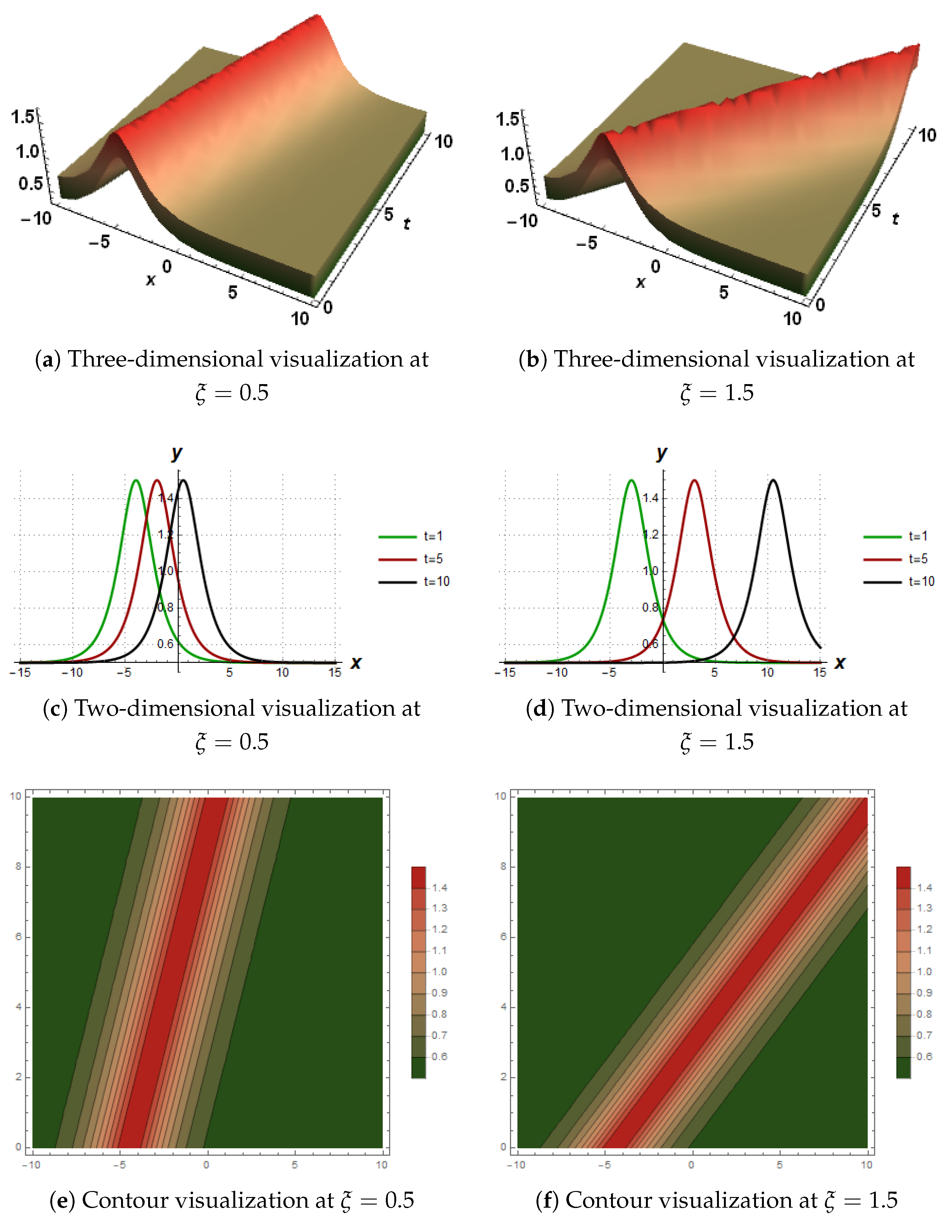
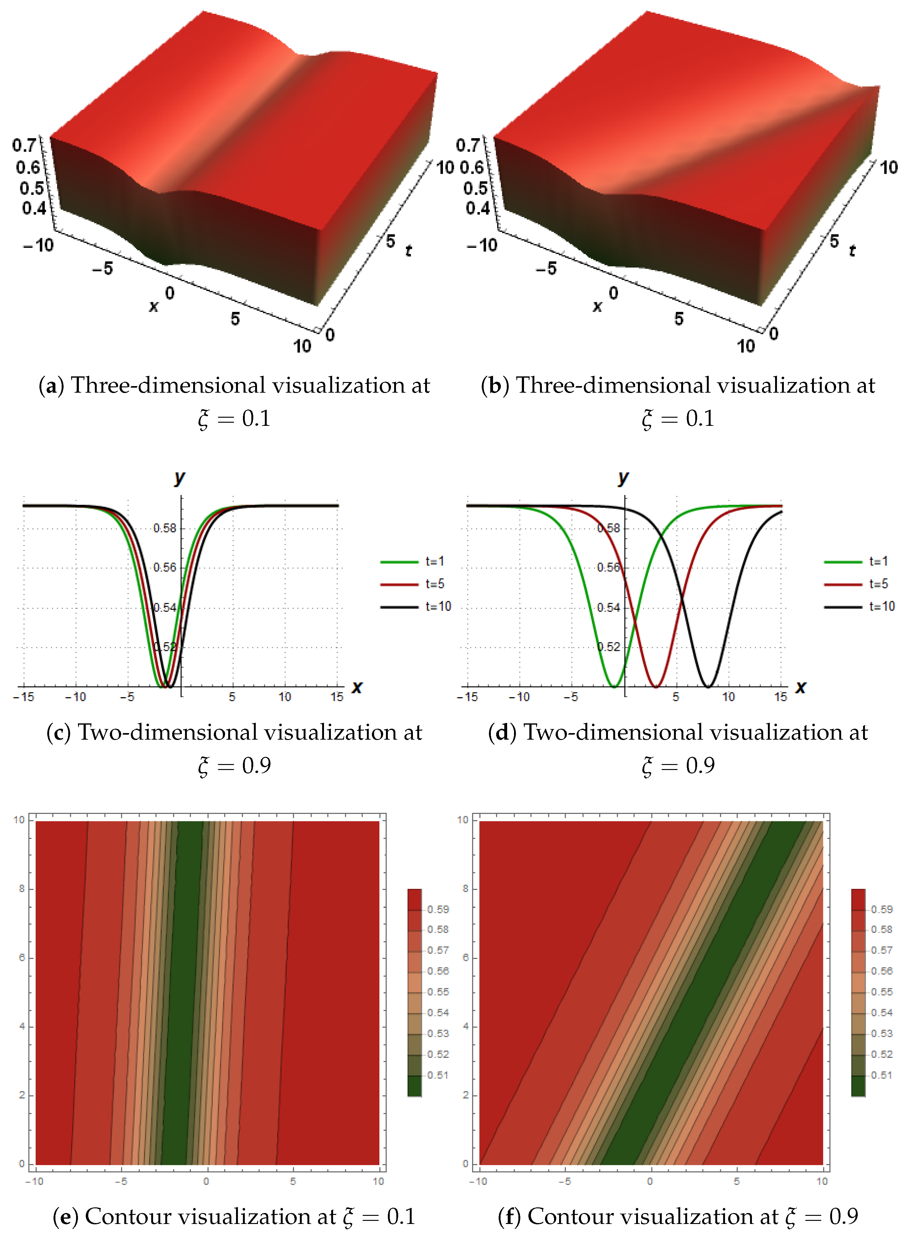
Geometric representation of the bright-type soliton solution. The x-axis represents the spatial coordinate, and the y-axis denotes the normalized amplitude, with a minor modification to the wave speed, as mentioned in

Table 1. Values of parameters with soliton solutions.

Solution No.	$\mathit{\xi }$	${\mathit{s}}_1$	${\mathit{s}}_2$	${\mathfrak{a}}_0$	${\mathfrak{a}}_1$	${\mathfrak{a}}_2$	${\mathfrak{a}}_3$	$\mathit{\phi }$	Results
${\mathrm{U}}_1^{\pm }(x,t)$	0.5, 1.5	0.5	...	...	...	...	...	4.5	Bright
${\mathrm{U}}_2^{\pm }(x,t)$	0.1, 0.8	0.1	...	...	...	...	...	2.5	Singular Kink
${\mathrm{U}}_3^{\pm }(x,t)$	0.1, 0.8	0.01	0.4	0.3	1.8	...	...	1.5	Bright Compacton
${\mathrm{U}}_4^{\pm }(x,t)$	0.1, 0.9	−0.1	0.5	...	...	...	...	2	Dark
${\mathrm{U}}_6^{\pm }(x,t)$	0.1, 1	−1	0.5	...	...	...	...	0.2	Kink
${\mathrm{U}}_8^{\pm }(x,t)$	0.1, 0.8	−1	...	...	...	0.3	0.4	0.2	Anti−Kink
${\mathrm{U}}_{10}^{\pm }(x,t)$	0.1, 1	−0.2	0.5	...	...	...	...	0.2	Cusped Periodic
${\mathrm{U}}_{11}^{\pm }(x,t)$	0.1, 0.5	−1	0.5	...	...	...	...	0.2	Periodic
${\mathrm{U}}_{14}^{\pm }(x,t)$	0.01, 1	0.4	0.1	...	...	...	...	1	Mixed-Kink, Periodic
${\mathrm{U}}_{17}^{\pm }(x,t)$	0.1, 0.5	2	...	...	...	...	...	0.2	Double Periodic

. In Figure 1 the color gradient indicates soliton intensity: red represents high amplitude and green indicates low amplitude. In 2D, fix the range of the x-axis to $-15\le x\le 15$. At $t=1$, the soliton is initially localized near the origin, showing maximum amplitude and narrow width. At $t=5$, the soliton broadens slightly and shifts along the x-axis, indicating forward propagation due to the convective term in the Cahn–Hilliard equation. At $t=15$, the wave peak has moved further along the x-direction, while the amplitude slightly decreases, reflecting energy dispersion and diffusive effects.

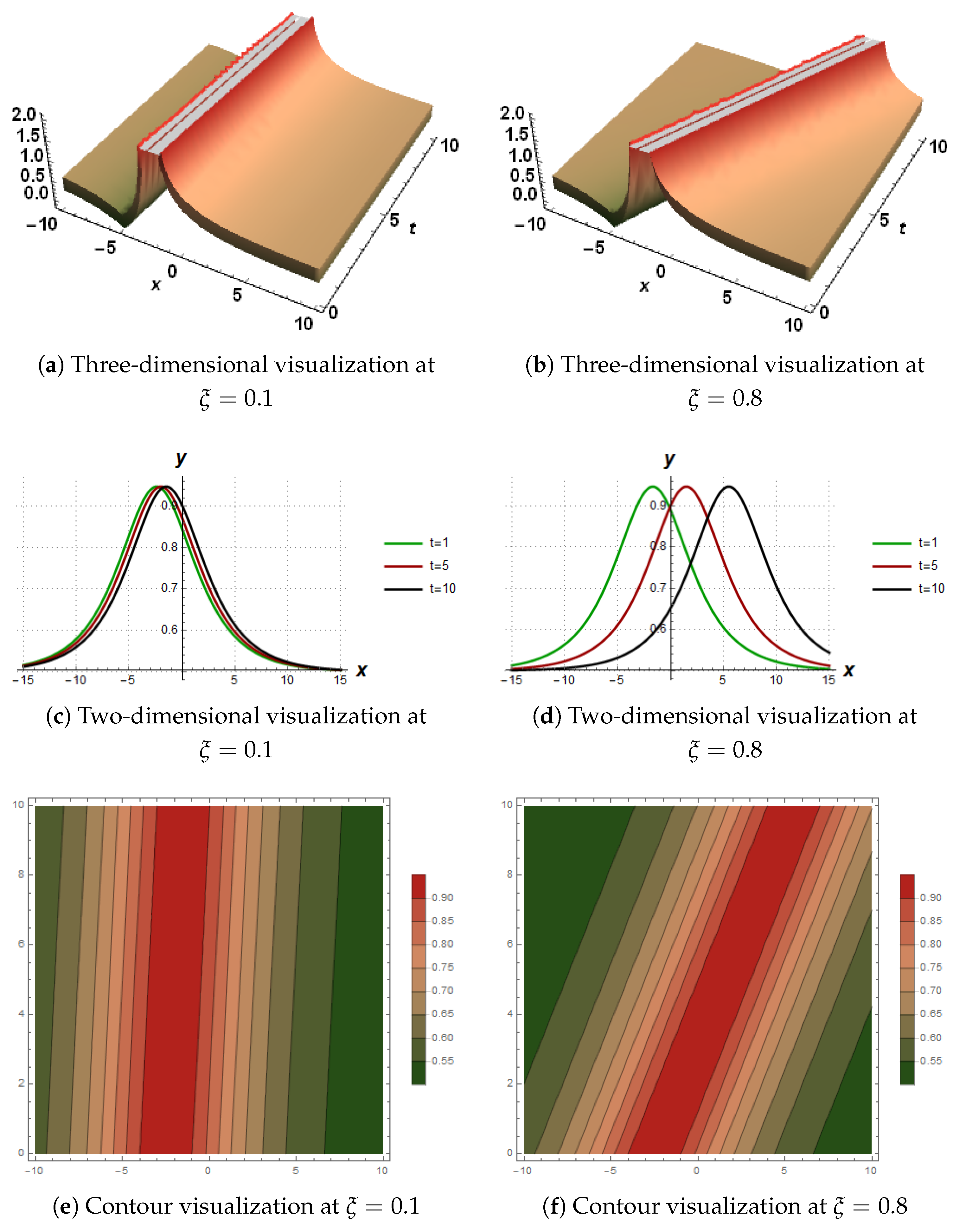
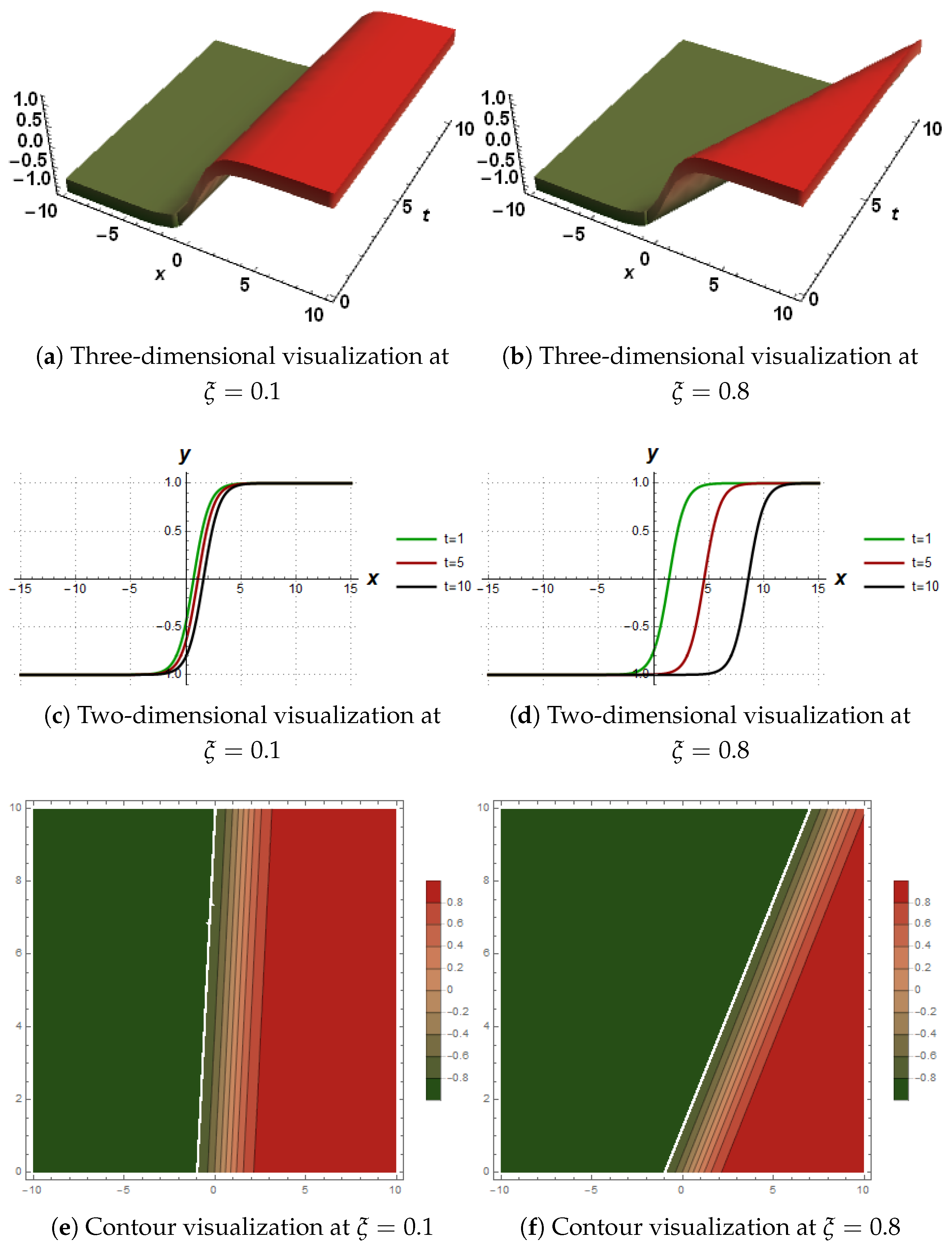
Geometric representation of a singular kink-type soliton. The x-axis represents the spatial coordinate, and the y-axis denotes the normalized amplitude, with slight modifications of the wave speed values, as listed in Table 1. In Figure 2 color gradient illustrates the soliton intensity, where red with white tones corresponds to higher amplitude levels and green tones represent lower values. Increasing the parameter $\xi$ enhances the steepness of the transition front, demonstrating the influence of nonlinear strength on the sharpness and propagation velocity of the kink profile. In 2D, the range of the x-axis is fixed as $-15\le x\le 15$. At $t=1$, the kink front is well-defined near the origin, marking a strong discontinuous-like transition between low and high amplitude states. At $t=5$, the kink moves forward along the x-axis, maintaining its asymmetric shape while slightly broadening due to the combined convective and diffusive effects of the Cahn–Hilliard system. At $t=15$, the wave front propagates further in the positive x-direction, showing a smoother transition zone and reduced gradient steepness, indicating the dissipative influence of diffusion on the singular kink geometry.

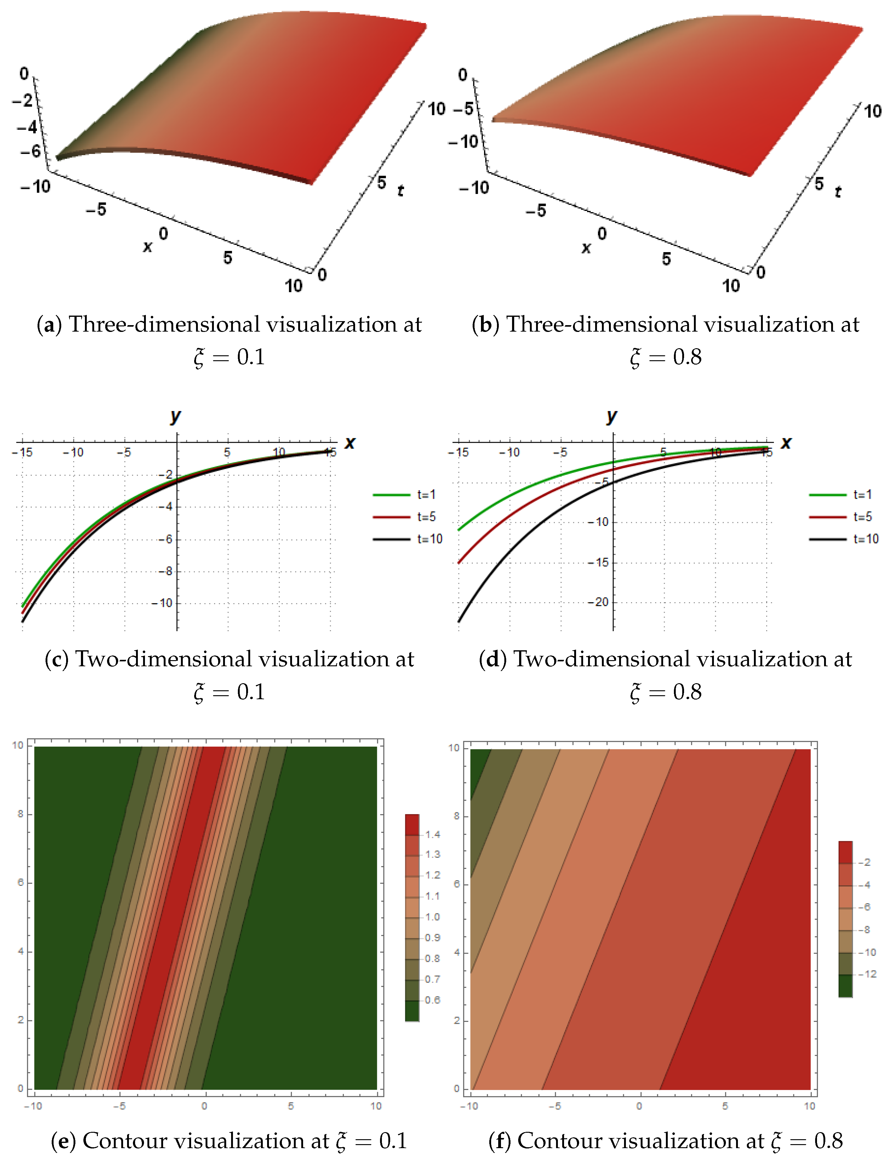
Geometric representation of the bright compacton-type soliton solution. The x-axis range is fixed as $-15\le x\le 15$. In Figure 3 the color gradient indicates soliton intensity, where red to green tones denote regions of high amplitude to low amplitude zones. The compacton-type soliton exhibits a finite spatial support; its amplitude remains strictly localized within a bounded region, after which it abruptly drops to zero. In the 2D representation, the soliton profile is positioned predominantly along the negative y-axis, extending through the fourth to third quadrants, which visually reflects its phase inversion and antisymmetric propagation behavior. At $t=1$, the compacton is well-localized near the lower half-plane with steep boundaries and high amplitude. At $t=5$, the soliton slightly expands and shifts, maintaining its compact structure but showing a mild lateral spread along the x-axis due to convective diffusion. At $t=15$, the compacton front propagates further along the x-direction, and its amplitude slightly decreases, illustrating the energy dispersion and diffusive broadening characteristics of the convective–diffusive Cahn–Hilliard dynamics.

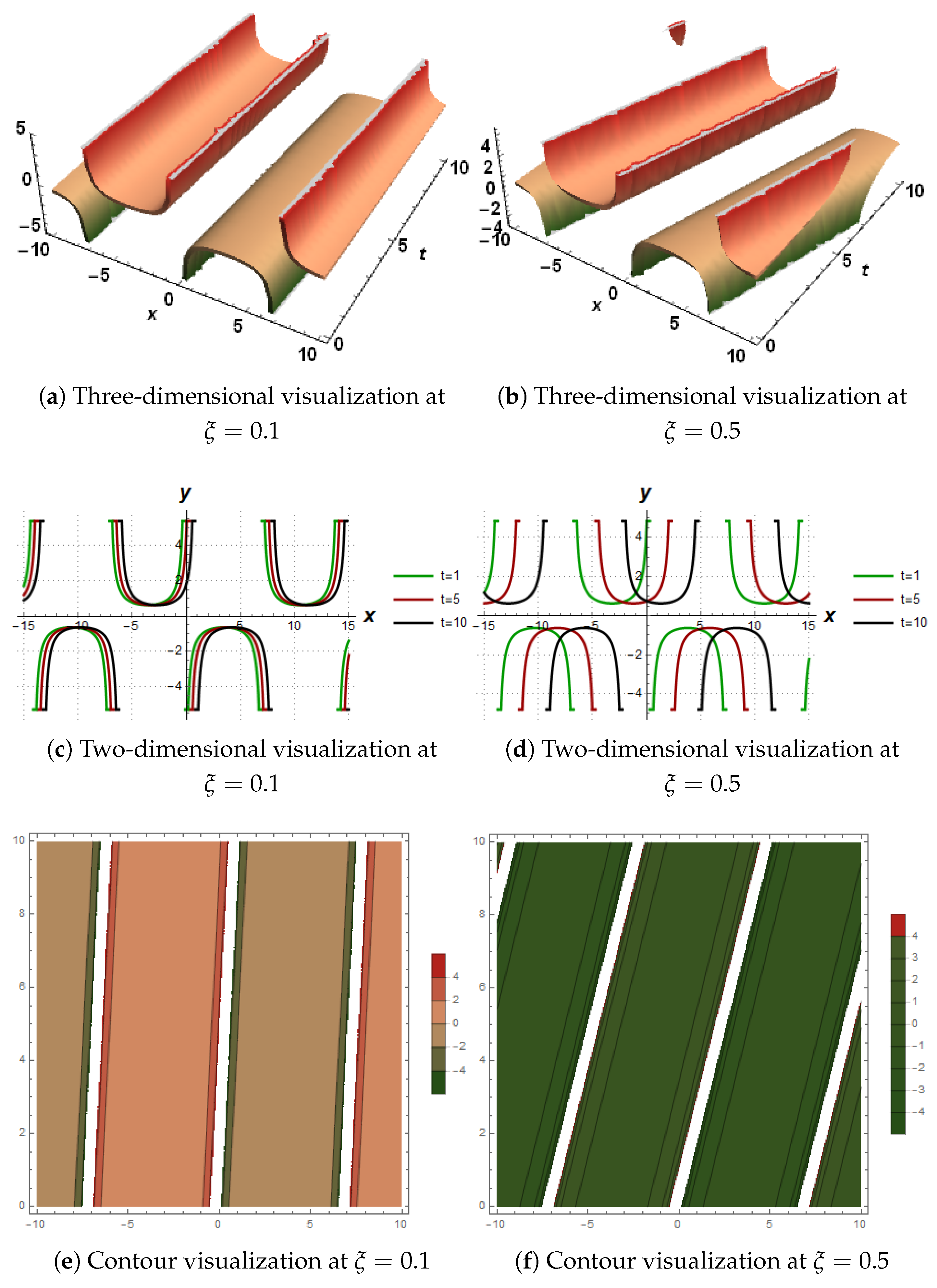
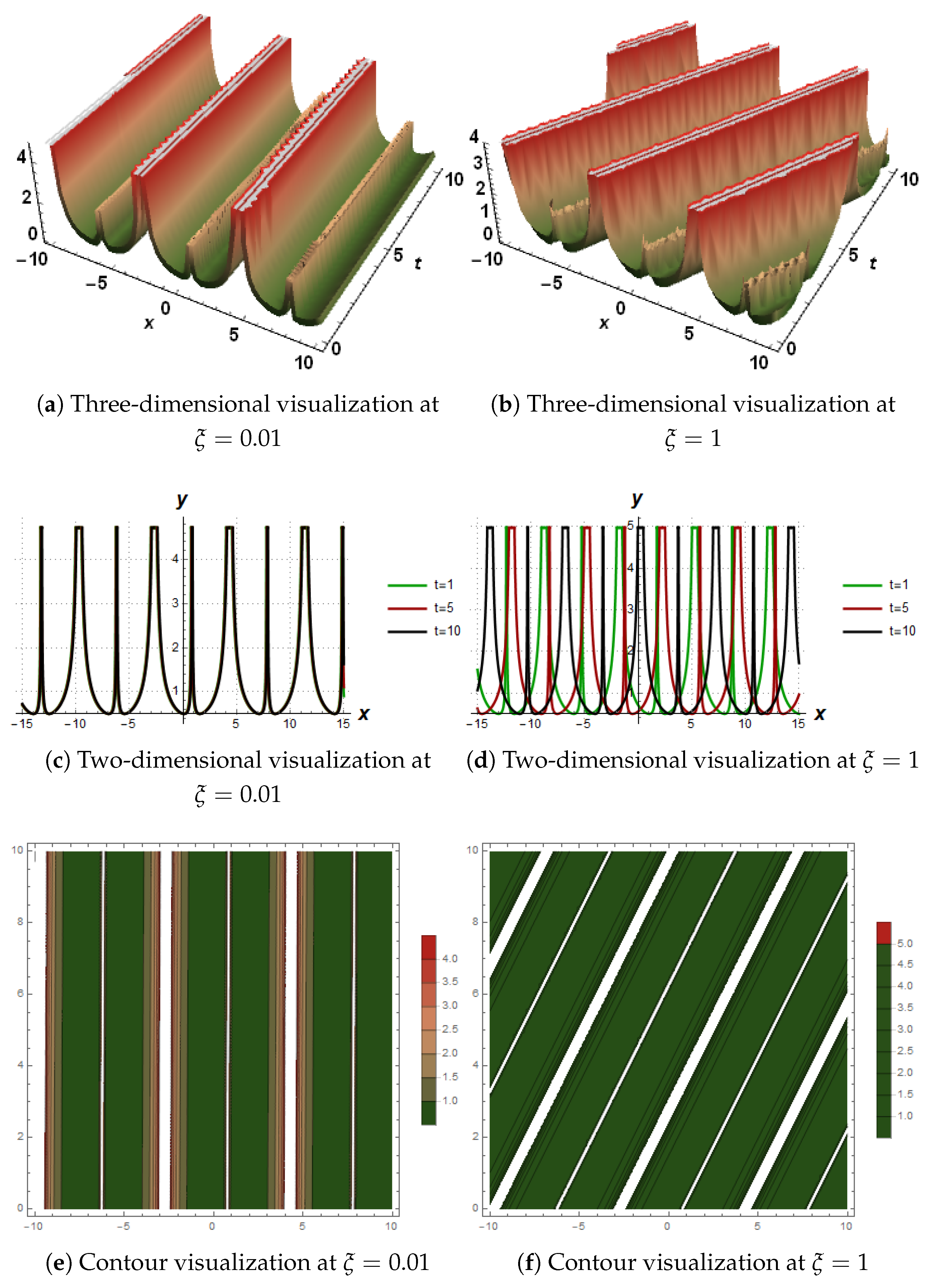
Geometric illustration of dark compacton-type soliton. The x-axis represents the spatial coordinate, and the y-axis denotes the normalized amplitude, with minor variations in wave speed values, as listed in Table 1. The x-axis range is fixed as $-15\le x\le 15$. In Figure 4 the color gradient indicates soliton intensity, where light-red tones denote regions of negative amplitude (troughs) and red tones indicate near-background amplitude zones. The dark compacton-type soliton exhibits finite spatial support, meaning its amplitude remains strictly localized within a bounded region, after which it abruptly returns to the background level. In the 2D representation, the soliton profile is positioned predominantly along the positive y-axis, extending through the first and second quadrants, which visually reflects its phase inversion and antisymmetric propagation behavior relative to the background. The confinement of the compacton in the positive y-domain signifies a phase-reversed nonlinear response, while its limited spatial width validates the non-dispersive, localized nature of dark compacton-type solitons.

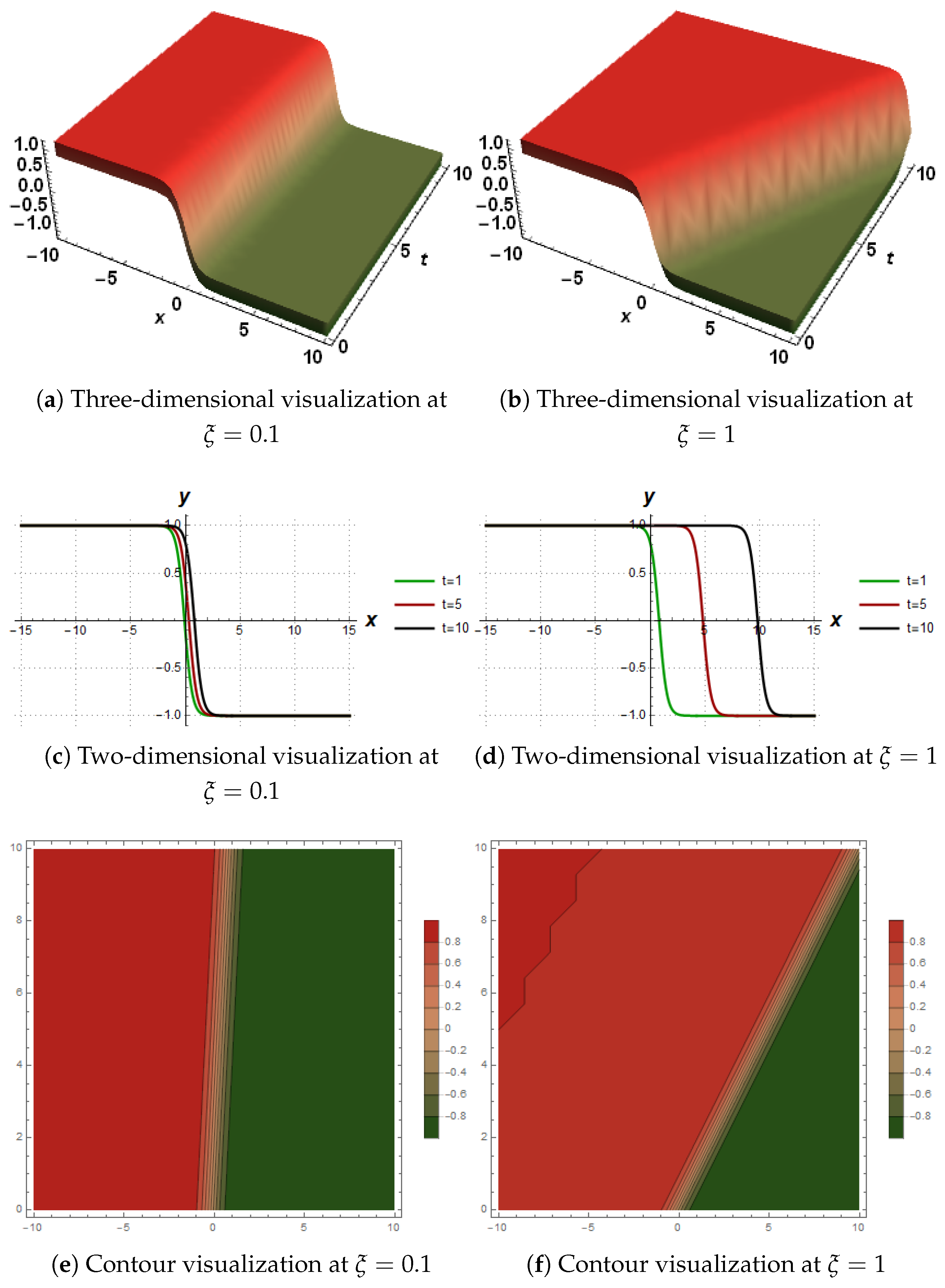
The kink soliton connects two asymptotic states of opposite signs and maintains a monotonic transition between them. The x-axis represents the spatial coordinate, and the y-axis denotes the normalized amplitude, with minor variations in wave speed values, as listed in Table 1. The x-axis range is fixed as $-15\le x\le 15$. The color gradient indicates soliton intensity, where red tones denote regions of higher amplitude and green tones indicate lower amplitude zones. For smaller $\xi$ the sub-figures (a,c,e) in Figure 5, the transition region is broader, corresponding to a gentle slope and slow propagation. For larger $\xi$ the sub-figures (b,d,f) in Figure 5, the soliton front is sharply localized, showing a nearly discontinuous jump between upper and lower states—characteristic of high-velocity kink waves. The geometrical differences among the panels, therefore, arise directly from the nonlinear coupling between the propagation velocity and the spatial compression parameters.

Geometrically, the anti-kink soliton transitions mean that the soliton wave moves diagonally from the first quadrant (positive amplitude) toward the third quadrant (negative amplitude) in the plane. This downward transition corresponds to a phase-reversed propagation, preserving the soliton’s localized nature but inverting its polarity, where the green tone corresponds to the lower amplitude region and the red tone represents the higher amplitude region. The propagation parameter $\xi$ continues to control the steepness and localization of the wave front. For small $\xi$, the anti-kink is broad, showing a smooth slope between the two states. $\xi$ increases, the transition region becomes narrower, and the slope becomes steeper, producing a sharply localized step-like geometry that crosses the origin from positive to negative amplitude. Thus, in Figure 6 the sub-figures (a,c,e), and (b,d,f), respectively, depict slow, moderate, and fast anti-kink propagation cases. The kink and anti-kink solitons are topological mirror states, carrying equal but opposite topological charges.

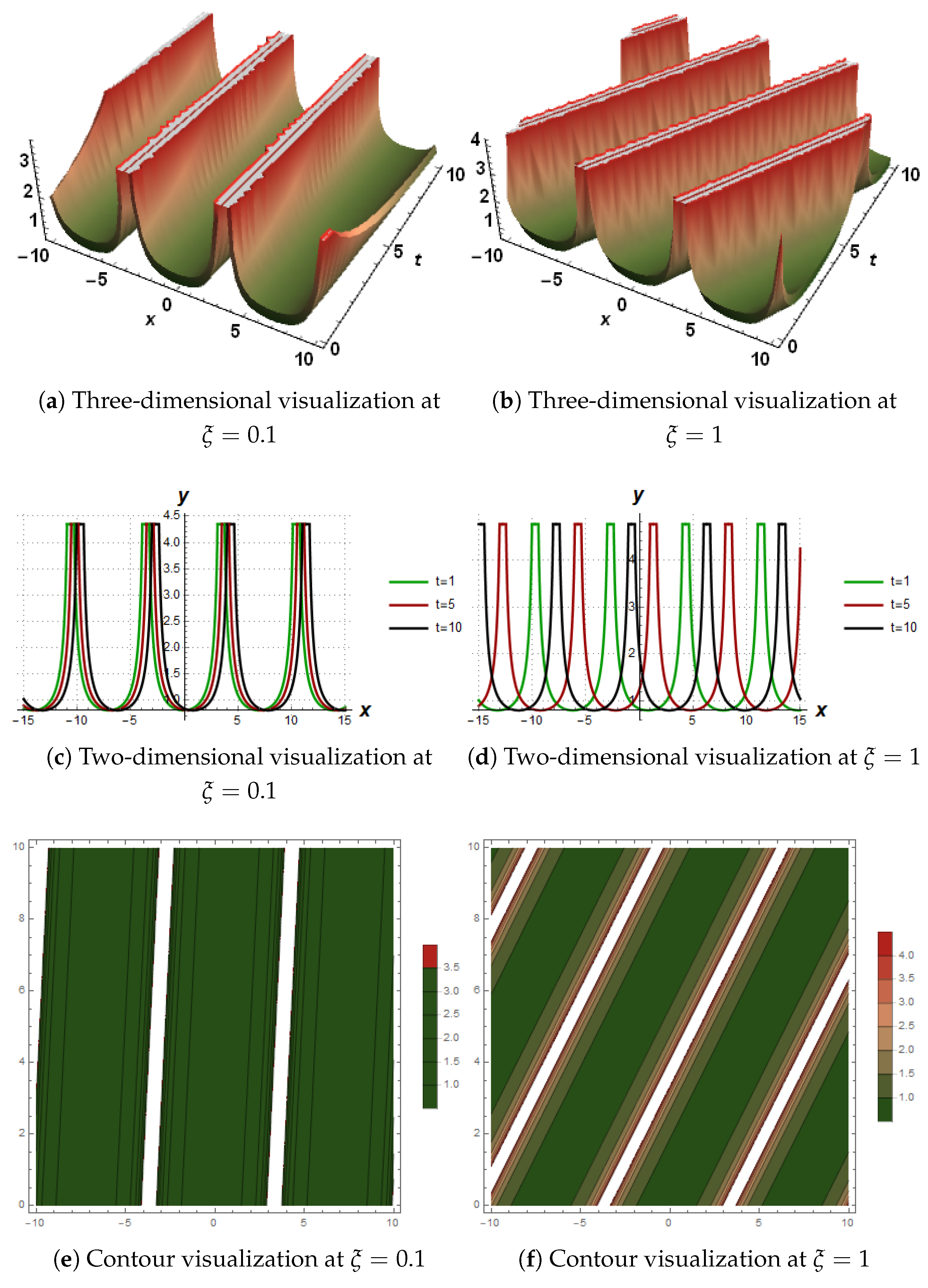
Geometrically, the cusped periodic-type soliton exhibits a train of spatially periodic waveforms characterized by sharp peaks (cusps) and finite amplitude oscillations. Unlike smooth periodic or sinusoidal solutions, the cusped periodic soliton possesses non-differentiable points at its maxima. In Figure 7 the 2D representation, the periodic soliton pattern extends symmetrically across the x-axis, showing alternating crests and troughs along the amplitude (y-axis). The solution remains bounded and recurrent, representing a stable nonlinear wave train rather than a single localized pulse. At $t=1,5,10$, the cusped wave train is well defined, with sharp, periodic peaks and uniform spacing between adjacent crests; they move and separate according to time. The alternating bright and dark stripes correspond to positive and negative amplitude regions, respectively. Warmer colors indicate higher amplitude near the cusp peaks, while green marks the low-amplitude troughs. The narrowing of the bright stripes with increasing $\xi$ demonstrates enhanced energy concentration and reduced spatial period.

The mixed kink–periodic-type soliton exhibits a hybrid nonlinear structure, combining the monotonic transition feature of a kink soliton with the oscillatory modulation characteristic of a periodic wave. Some parabolic oscillations appear in the first and second quadrants, representing the positive phase of the periodic component, while others are located in the third and fourth quadrants, corresponding to the negative phase of oscillation. This spatial distribution illustrates the antisymmetric and alternating nature of the mixed kink–periodic soliton. For smaller $\xi$ in sub-figures (a,c,e), in Figure 8 the kink front is broad and the oscillations are gentle and widely spaced. For larger $\xi$ sub-figures (b,d,f), in Figure 8 the periodic oscillations dominate, and the kink front interfaces with fine ripples, indicating strong nonlinear dispersion.

Geometrically, the x-axis represents the spatial coordinate, and the y-axis denotes the normalized amplitude, with minor variations in wave speed values, as listed in Table 1. In Figure 9 the x-axis range is fixed as $-15\le x\le 15$. The color gradient indicates soliton intensity, where red tones represent a higher amplitude region, and green tones denote a lower amplitude region. The mixed kink–periodic-type soliton exhibits a hybrid nonlinear profile, combining the monotonic phase transition of a kink soliton with the oscillatory and repeating structure of a periodic wave. At $t=1$, the soliton displays a well-defined kink front with visible periodic ripples. At $t=5$, mild lateral spreading occurs along the x-axis due to convective diffusion, but the overall hybrid structure remains preserved. At $t=15$, the wave propagates further in the x-direction, the amplitude remains the same, and diffusive broadening is consistent with the convective–diffusive Cahn–Hilliard dynamics.

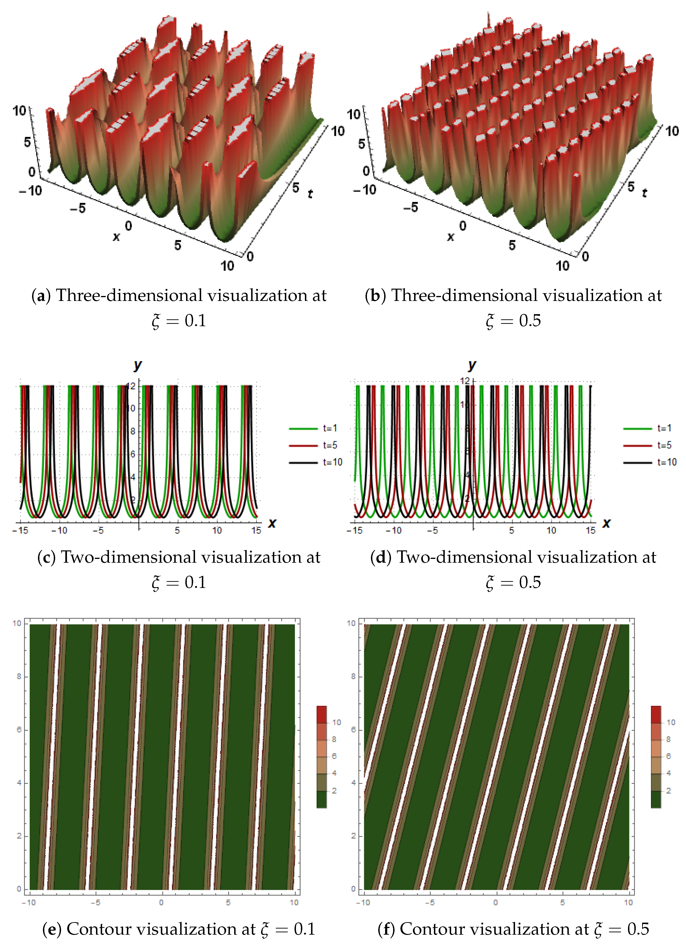
The double–periodic-type soliton describes a nonlinear periodic wave that exhibits dual oscillatory characteristics in both spatial and temporal dimensions. The 3D plots sub-figures (a,b), in Figure 10 that waveform exhibits a double-rippled surface with distinct parallel ridges along both directions that become denser or more separated, depending on the propagation parameter $\xi$. In 2D sub-figures (c,d), in Figure 10 the x-axis range is –$15\le x\le 15$ a clear oscillatory pattern repeats periodically with varying intensity, showing an overlap of two frequency modes. In Figure 10 contour plots (e,f), alternating green and red zones indicate regions of high and low amplitude; the intersection of periodic components forms a grid-like or diamond pattern, confirming double periodicity.

4. Results and Discussion

To highlight the importance of the convective–diffusive Cahn–Hilliard equation, we apply the modified Sardar sub-equation approach and precisely choose suitable values for the physical parameters. As a result of this conscious decision, we obtain new solutions that highlight the unique characteristics of the problem. We also introduce a set of carefully constructed graphs to further investigate the physical consequences of these solutions. These illustrations highlight the unique features of the recently generated soliton solutions and offer deeper insights into the physical behavior of the equation, highlighting its applicability and contribution to the model’s overall comprehension. By adjusting the parameter values, different and new soliton solutions are obtained. In Figure 1, the bright soliton solution is illustrated. In Figure 2, the singular kink is drawn. In Figure 3, a bright compacton soliton is mentioned. Figure 4 contains the dark soliton, and Figure 5 contains the kink soliton. In Figure 6, the anti-kink soliton is illustrated. A cusped periodic soliton is mentioned in Figure 7. The class of periodic solitons is depicted in Figure 8, Figure 9 and Figure 10. The details of the parametric values are mentioned in Table 1. Using Maple, we derive the soliton solutions and plot these results with the help of Mathematica. The derived results are mentioned in the table.

The physical origin of the obtained soliton structures arises from the fundamental balance between nonlinear self-interaction and dispersive spreading present in the governing nonlinear evolution equation. This balance determines whether the system supports localized solitary waves, transitional fronts, or oscillatory periodic patterns. In Figure 1, Figure 2, Figure 3, Figure 4, Figure 5, Figure 6, Figure 7, Figure 8, Figure 9 and Figure 10, the two- and three-dimensional plots, together with contour representations, clearly demonstrate how this nonlinear–dispersive interplay shapes the geometry of each soliton type. By introducing the traveling-wave transformation $\varphi =x-\xi t$, the propagation parameter $\xi$ governs the speed and spatial deformation of the wave. Physically, larger values of $\xi$ enhance the nonlinear effect relative to dispersion, generating sharper, more localized energy packets, while smaller $\xi$ values allow dispersion to dominate, producing broader and smoother structures. This behavior is evident across the sub-figures, where the soliton profiles evolve from gentle undulations to steep wavefronts as the parameter varies. The color gradients further illustrate the energy distribution along the wave—warmer colors representing higher field intensity and cooler tones showing lower amplitude regions. Bright solitons reflect symmetric, energy-focused localization; kink and anti-kink solitons correspond to directional transitions between two equilibrium states, reflecting front-like propagation with clear physical relevance in optical, fluid, and magnetic systems; and mixed kink–periodic or double–periodic solitons emerge from partial dominance of dispersion, generating hybrid structures where periodic oscillations interact with localized wave fronts. These geometric and physical characteristics confirm that parameter modulation directly governs the underlying physical mechanisms, and they demonstrate that the modified Sardar sub-equation technique reliably captures a wide spectrum of nonlinear wave processes inherent to the considered model.

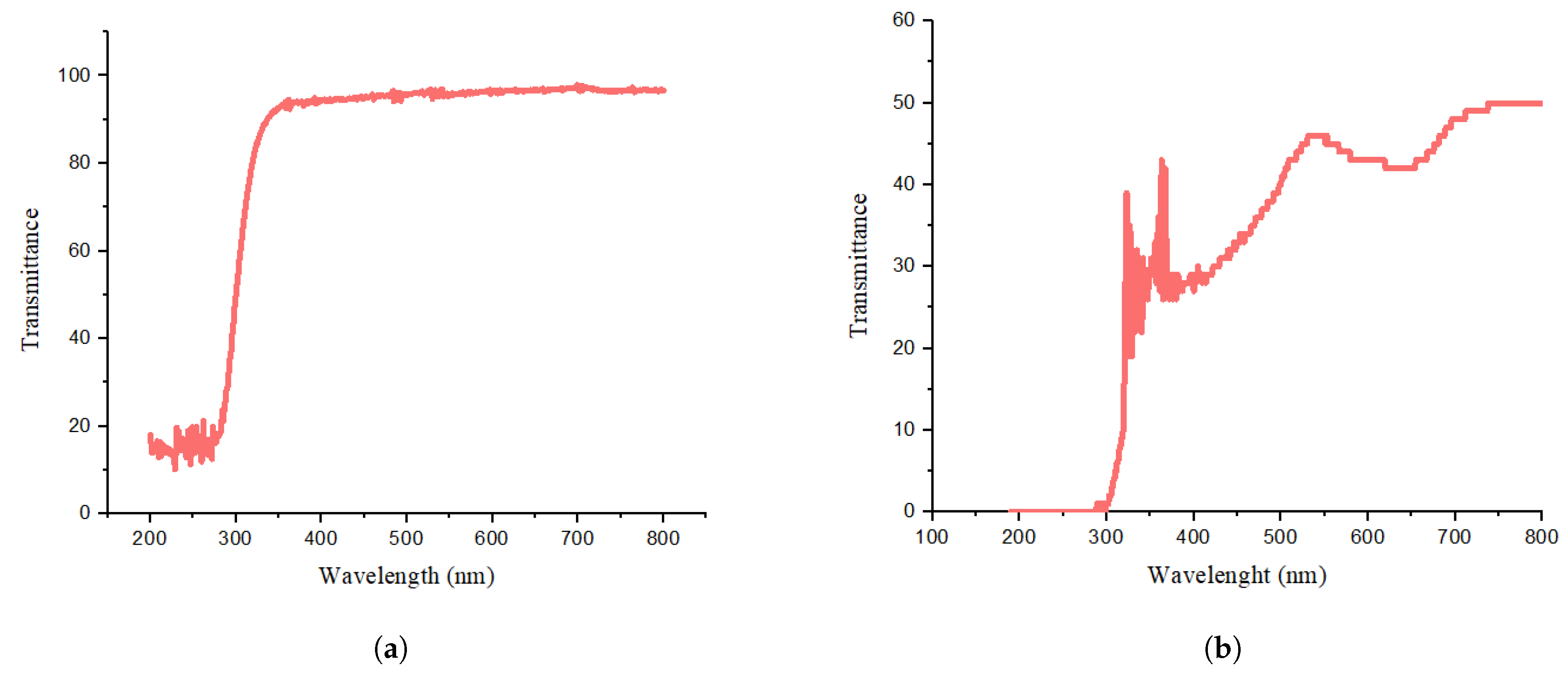
In this work, the obtained UV–Vis spectra of CuO thin films display periodic transmittance variations in the visible region, indicating interference and phase modulation effects. These periodic behaviors are in qualitative agreement with the theoretical soliton profiles derived from the convective–diffusive Cahn–Hilliard equation, where parameter variation reproduces similar oscillatory waveforms. This correlation highlights the innovative aspect of the study linking analytical soliton theory with experimentally observed optical phenomena in copper oxide thin films, a connection that has not been reported in earlier research [23].

The Cahn–Hilliard equation and its modified forms have proven to be powerful tools for modeling phase separation and interface evolution in diverse physical systems. Beyond its well-known role in materials science and fluid dynamics, this model provides valuable insights into pattern formation and morphological transitions driven by diffusion and convection effects. For example, in metal alloys, compositional fluctuations under cooling can trigger spontaneous phase segregation, while in polymer blends, molecular incompatibility gives rise to microstructure formation. Similarly, in thin-film systems, the Cahn–Hilliard framework explains how surface tension and dewetting mechanisms generate ordered nanoscale patterns. This complementary perspective highlights that the model not only captures separation kinetics but also describes the self-organization processes underlying the emergence of complex geometrical structures in real materials.

5. Experimental Work

The convective–diffusive Cahn–Hilliard equation is a strong model that has applications in materials science, along with fluid dynamics, among other domains. It is very important in the simulation of phase separation in metals, polymers, and other materials, and also describes the mixing of fluids of varying densities or viscosities [24]. This concept has crucial applications and is very useful in creating thin films of various materials. This article uses copper oxide material to examine the optical properties. These compounds are intensively investigated because of their distinct physical and chemical features. UV-Vis spectroscopy can analyze the optical properties of copper oxide deposited on a borosilicate glass substrate [25,26]. 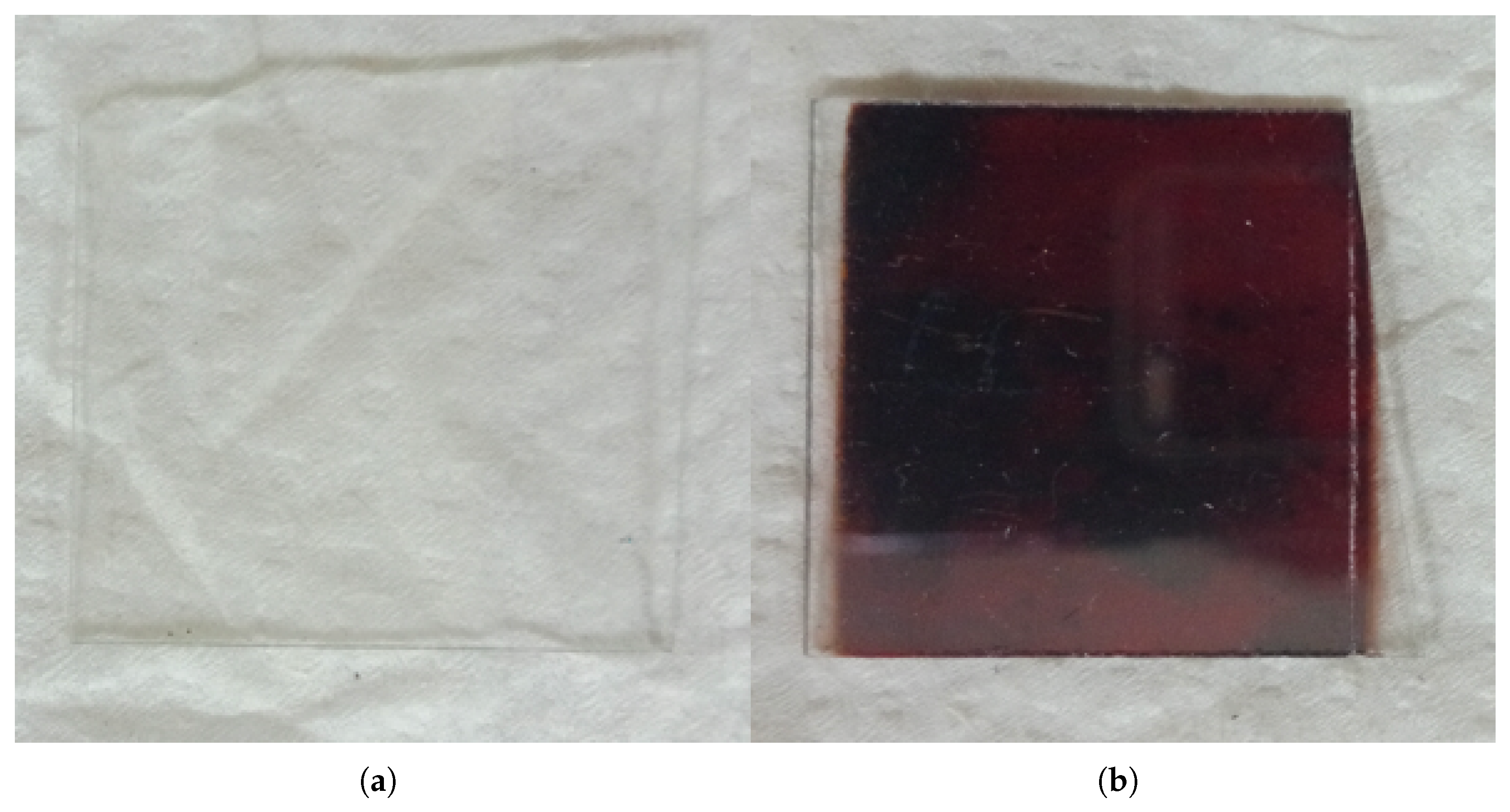In Figure 11, part (a) is a simple borosilicate glass, and in part (b), copper oxide is deposited on simple borosilicate glass.

A spectrophotometer is used to examine the optical properties of the generated thin films, with an emphasis on transmittance in the ultraviolet–visible (UV-Vis) spectral region. Figure 11, part (a), shows the transmittance spectrum of a basic borosilicate glass substrate, demonstrating its inherent transparency within this spectral window. This transparency is an important feature for many optical applications, as it enables efficient light transmission. Part (b) shows the transmittance spectrum of a copper oxide thin film formed on a borosilicate glass substrate. A pronounced absorption edge is visible in the UV region, around 300 nm. This dramatic drop in transmittance marks the onset of strong absorption due to electronic transitions within the copper oxide material. CuO thin films were synthesized using a thermal evaporation system operating under a base pressure of approximately $5\times {10}^{-6}$ mbar. High-purity CuO powder $(99.99\%)$ served as the source material. During deposition, the substrate-to-source distance was maintained at 12 cm, and the deposition rate was carefully controlled within the range of 1–2 A/s to ensure uniform and stable film growth. The resulting CuO thin films exhibited a thickness between 150 and 180 nm. Optical measurements revealed that the films possess solid transmittance characteristics in the visible region, with an average transmittance exceeding $80\%$, confirming their high optical quality and uniform crystalline nature.

In soliton solutions, the input parameters should be the optical characteristics obtained from UV-Vis spectroscopy. This will enable us to predict quantitatively how the optical characteristics of the film impact the propagation of the soliton. The dispersion of light inside the film is mostly determined by the material’s refractive index, which is correlated with transmittance and absorption. One of the most important elements is the dispersion, which balances nonlinearity to form solitons. This UV-Vis data offer important information about the film’s optical characteristics, which is necessary for understanding possible soliton propagation. The strong transmittance above 400 nm indicates that this area might allow both bright and dark solitons, while more characterization of nonlinear optical characteristics is required. The absorption edge and overall spectral shape offer information on the material’s electronic band structure, which is crucial to kink soliton formation, whilst the film’s optical features, especially when combined with any periodic thin film structures, might impact the behavior of periodic solitons. However, further approaches are required to completely link these optical features with the actual presence and dynamics of the various soliton types (bright, dark, kink, and periodic) inside the CuO thin film [27,28]. In Figure 12, part (a) shows the transmittance of simple glass, and part (b) shows the wave behavior when copper oxide is deposited on the substrate.

The theoretical soliton solutions obtained using the modified Sardar sub-equation method exhibit periodic and quasi-periodic behaviors that closely resemble the oscillatory transmittance and absorbance patterns observed in the UV–Vis spectra of the CuO thin film. The peaks and troughs in the simulated profiles correspond to the optical interference fringes generated by film thickness and refractive index variation. Although a detailed quantitative fitting between theory and experiment is beyond the present scope, the qualitative agreement between the periodic characteristics supports the physical relevance of the proposed model.

6. Conclusions

In this study, the modified Sardar sub-problem technique was successfully applied to obtain exact bright, dark, kink, and periodic soliton solutions of the convective–diffusive Cahn–Hilliard equation. The parametric analysis revealed that variations in the propagation parameter influence the geometry and localization of the derived solitons. The dynamic characteristics and useful applications of the derived soliton solutions have been successfully illustrated through in-depth graphical simulations using Mathematica and Origin. Moreover, experimental UV–Vis measurements of copper oxide (CuO) thin film showed an absorption edge around 380–410 nm and a band gap near 2.3 eV, which qualitatively agrees with the periodic features predicted by the theoretical model. This work establishes a direct link between nonlinear soliton dynamics and optical characteristics of thin-film materials. The proposed analytical framework can be extended to other nonlinear PDEs relevant to phase separation and material modeling.