Article

Tool-Life Estimation Model in Milling Processes Using Multi-Head Cross-Covariance Attention Fusion-Based Dilated Dense Bi-Directional Gated Recurrent Unit

by
Hisham Alkhalefah
1,2
1
Advanced Manufacturing Institute, King Saud University, P.O. Box 800, Riyadh 11421, Saudi Arabia
2
Industrial Engineering Department, College of Engineering, King Saud University, P.O. Box 800, Riyadh 11421, Saudi Arabia
Mathematics 2025, 13(23), 3798; https://doi.org/10.3390/math13233798
Submission received: 28 October 2025 / Revised: 19 November 2025 / Accepted: 22 November 2025 / Published: 26 November 2025
(This article belongs to the Special Issue Artificial Intelligence for Fault Detection in Manufacturing)

Abstract

When performing the milling process, it is essential to consider the life estimation and availability of the milling tool to achieve a reliable and optimized result at a lower cost. It is necessary to monitor the tool’s condition during the milling process due to its inherent wear nature. In earlier times, visual inspection was used to assess the condition of the milling tool, and it was considered a complex and specialized task. Due to this issue, the milling process requires further investigation. In the manufacturing and automation industry, deteriorated milling tools have led to several challenges, including a decline in product quality, reduced equipment utilization, and increased costs. The tool wear prediction is a challenging and complex task, as it includes several variables. The existing framework for tool condition monitoring, in terms of the degree, typically falls short in terms of real-time prediction and accuracy. Hence, in this research, a tool-life estimation model is developed to minimize unexpected failures during the milling process using deep learning techniques. Initially, the data are collected from benchmark sources. The statistical features, deep features via fuzzy autoencoders (FAEs), and t-Distributed Stochastic Neighbor Embedding (t-SNE)-based features are extracted from the input data to capture various information related to the machine. These features are passed to the proposed multi-head cross-covariance attention fusion-based dilated dense bi-directional gated recurrent unit (MCF-DD-BiGRU) for accurate prediction of tool life. The input features are fused using a multi-head cross-covariance attention mechanism to enhance the representation of interdependencies among features. The DBi-GRU network processes the fused features to improve the accuracy of tool-life prediction for milling machines. The prediction efficiency of the implemented model is compared with the existing models to ensure its effectiveness.

1. Introduction

In the automation and manufacturing industries, a common issue known as machine tool wear can result in higher costs, lower-quality outcomes, and reduced equipment utilization. Therefore, it is challenging to make efficient and accurate predictions of machine tool wear, which is essential for maintaining productivity and machine health [1]. Some of the categorization involved in the tool condition monitoring is fault type determination, fault detection, and estimation of Remaining Useful Life (RUL). It is determined using the prognostics methods [2]. In recent times, prognostics has emerged as a research field to identify tool breakage. The input sensory data are taken by the prognostic model, which is considered to be the health statement problem [3]. In general, this prognosis is determined using steps such as identifying indicator failure, constructing the health index, and estimating the present state. In the prognostics, the analysis or prediction of RUL is the main target, where the time machine can safely work without any breakage [4]. The health index of the tool wear obtains the estimation of RUL for the machine. Product quality can be compromised when there is severe tool wear, resulting in a higher rejection rate and potentially causing accidents in machine tools [5]. Production efficiency is improved through effective tool management, which helps minimize maintenance and operational costs. However, adopting an overly protective strategy does not fully leverage the value of the tool. Additionally, time consumption increases due to unnecessary downtime caused by tool changes [6].
In the machining process, the most active component is the cutting tool, which inevitably wears out as it separates the metal material, ultimately causing failure. The replacement of the cutting tool must happen before the inability to guarantee the quality [7]. The accurate forecasting of tool RUL not only determines replacement but also extends the tool’s lifetime, ensuring savings in machining costs and reducing failures [8]. During the machining process, the workpiece is in contact with the cutting tool, where the quality of the outcome is directly influenced by the degree of wear on the tool. Generating tool changes based on personal experience tends to lead to poor judgment [9]. Acute tool wear can cause tool fracture, chatter, and chipping, which generally harm both the operator and the machine tool. Therefore, it is crucial to determine the tool’s condition during actual machining to reduce processing costs and unnecessary downtime due to tool wear [10]. To mitigate the expenses in the manufacturing sector, it is essential to perform tool condition monitoring. Most tool failures are caused by tool downtime, indicating that tool wear has a direct impact on the quality and precision of the machined surface [11].
Several physics-based approaches and data-driven models have been developed for accurate tool wear prediction. In this era of Artificial Intelligence (AI), machine learning (ML) is applied in various domains [12,13,14]. The utilization of advanced AI approaches for developing tool health classification increases detection accuracy in tool wear, thereby enhancing productivity and reducing maintenance [15,16]. The traditional prediction methods used for milling tool wear typically face limitations in producing accurate results due to the underlying system dynamics. The machining process is stopped by the straightforward model, which removes the tool and provides an optical measurement for the precise determination of the wear area. However, the earlier models have a significant impact on operational efficiency [17]. In processing the sensor time series, the LSTM achieved a unique advantage; however, it has a limitation in performing feature extraction [18]. Therefore, it is crucial to develop an advanced strategy that addresses all the limitations in earlier research. Hence, a new tool-life estimation model is created in this work through the involvement of a deep learning model.
Motivation and research gaps of the proposed work: The motivation for this research work stems from the growing need to accurately forecast tool life and eliminate unexpected tool failures in modern milling operations, which directly impact cost, productivity, and machining quality in the manufacturing sector [18]. The conventional approaches to tool-life estimation, such as physics-based models and empirical methods, primarily rely on limited experimental data and fail to capture the dynamic, nonlinear, and intricate behavior of real-time machining conditions [18]. Even with the development of machine learning and deep learning approaches in recent years, the majority of models still suffer from specific problems, including the limited fusion of multimodal sensor data, inadequate feature representation, and insufficient modeling of temporal dependencies in the data [18]. For instance, most of the existing approaches utilize only handcrafted or statistical features extracted from current or vibration signals, which overlook the deeper correlations among signals from distinct sensors [18]. Likewise, the precious deep learning models such as CNNs, LSTMs, and basic GRUs have improved accuracy but mostly fail to efficiently combine heterogeneous datasets or capture cross-feature dependencies crucial for reliable tool wear and remaining functional life prediction [18]. To address these problems, the existing work presents a novel MCF-DD-BiGRU technique. The motivation behind this mechanism is to design a highly intelligent and comprehensive model capable of integrating diverse features, such as statistical deep and t-SNE-based, while learning complex interdependencies among them via an advanced multi-head cross-covariance attention method. This fusion enables the technique to better understand the relationships among sensor modalities, such as current, vibration, and force signals, which are mostly treated independently in previous works. Moreover, the integration of a dilated dense Bi-GRU model enhances the technique’s capability to capture both long-term and short-term temporal dependencies in sequential data, thereby improving the accuracy of tool-life estimation. Hence, this research addresses the limitations of conventional approaches by proposing a hybrid, robust deep learning model that not only enhances prediction accuracy but also provides high reliability and generalizability for real-world industrial milling applications.
The significant contributions of this work are detailed below.
  • To implement an intelligent tool-life estimation framework in the milling process by training efficient deep learning technology to predict the tool wear. This framework leverages multi-domain feature extraction to extract significant features, thereby achieving higher prediction accuracy. This prediction provides the status of RUL or tools’ current wear to perform proper tool changes at the right time. This tends to improve the machining precision and reduce the unplanned downtime in an intelligent manufacturing system with real-time monitoring.
  • To convert the raw data into meaningful input features, this work performed the multi-domain feature extraction process for accurate tool-life prediction. The feature extraction utilizes statistical, t-SNE, and FAE to refine the information available for the model. This process effectively generates clear visual clusters of data points from the given data. This process automatically captures the relevant and comprehensive information from complex data for achieving better predictive maintenance.
  • To develop an MCF-DD-BiGRU for tool-life estimation with multi-head feature fusion. The system utilizes the MCF as the feature learner to determine the given three sets of features completely. Further, the DD-BiGRU performs the estimation based on the fused feature and delivers the present tool value. The model led to higher prediction accuracy, which is suitable for tool condition monitoring. Based on the outcome, the tool wear value can be monitored in real-time and make an intelligent decision to improve the processing quality of the product with a minimum rejection rate.
The remaining work is as follows. Section 2 details the existing literature on tool-life estimation. Section 3 provides an overview of the designed methodology along with a dataset description. Section 4 determines a different set of feature extraction processes. Section 5 details the design model of the final tool estimation approach. Section 6 provides the experimental setup and the comparative analysis. Finally, Section 7 concludes the work with future directions.

2. Literature Review

This section describes and assesses existing works related to machine learning applications for predicting machine tool life.

2.1. Related Works

Khan et al. [19] have suggested using the LSTM model to determine time series sequential data. The suggested model has the potential to achieve an impressive and accurate outcome. The experiments were conducted for different workpiece materials, including brass, aluminum, and mild steel, to achieve a precise prediction. Elminir et al. [20] have designed a tool wear prediction approach for milling machine cutters incorporating the AE and the LSTM. Several steps were involved in the framework, including correlation analysis and multi-domain feature extraction. The target tool was predicted by training, testing, and validating the developed model. The RUL value was estimated by comparing with the value of the predicted tool wear.
Che et al. [21] designed the hybrid method, where the design construction involved three major components to improve the precision of prediction. The most relevant features were extracted through the filtering process from the raw signals, improving the model’s interpretability. An experimental analysis was conducted to evaluate the features and capabilities of the proposed technique. Shah et al. [22] recommended the Morlet wavelet model for determining the vibration signals from the scalogram. The corresponding wavelet functions were selected by applying the relative energy criterion. The stacked LSTM effectively predicted the tool wear better than other approaches.
Wang et al. [23] have adopted the prediction model using the hybrid network with the involvement of the multi-channel fusion. During the tool-life cycle, the multi-source sensor signals were collected, and the computer vision-based feature extraction was performed. The designed approach improved the efficiency of the RUL prediction model. Kamat et al. [24] developed a deep learning-based system for the prediction process to evaluate the tool life by detecting the wear onset. The tool wear onset was estimated by the hybrid model, and its remaining useful life was predicted.
Li et al. [25] suggested the tool RUL prediction model using a convolutional stacked network. The model fused the gathered multi-sensor signal during the cutting process and then generated signal feature mapping based on the tool value. The experiment on milling revealed that the implemented framework not only improved the RUL prediction but also achieved better generalization ability. Kaliyannan et al. [26] adopted the RL-based model to monitor the condition of the tool in the milling process. The tool condition was classified by employing a deep learning model based on the vibration sensor. The outcome showed that the suggested model outperformed the existing models with enhanced efficiency for the overall process.

2.2. Research Gaps and Challenges

Manufacturing sectors are growing due to the integration of automated and intelligent production processes provided by technological advancements. Maintaining the milling machines helps to improve their performance by handling challenging and complex processing issues. However, tool damage or malfunction can affect the processing performance. Therefore, monitoring the tool’s state during processing is essential to address major tool failures. If the machine components are affected, this directly impacts the production of expensive products. Researchers have developed various deep learning techniques to predict the lifetime of milling tools, and some of the common challenges in the existing works are provided below.
  • Existing approaches, such as SVM or CNN, are not feasible for capturing the complex and non-linear relationships in the sensor data collected during the milling process. Moreover, they are less efficient in analyzing unstructured feature spaces and high-dimensional data.
  • Most of the models have obtained less prediction accuracy due to the loss of necessary information. Existing models cause this, as they only consider single-feature modalities.
  • Issues such as inter-feature correlations and suboptimal utilization of diverse data sources may occur in conventional models, as they do not incorporate efficient feature fusion mechanisms.
  • The computational complexity and memory consumption of the LSTM model are high. Both past and future signal patterns associated with tool wear are not precisely captured by the existing techniques.
Table 1 shows the features and challenges of some of the reported methodologies in the literature.

3. Significance and Overview of the Proposed Tool-Life Estimation Process in Milling

This section explains the importance of predicting tool life in milling. Furthermore, the proposed method is explained in detail.

3.1. Significance of Estimating the Tool Life in Milling

Tool-life estimation in the milling process involves several prediction methods, which forecast the useful life of the tool by considering factors such as workpiece material, depth of cut, cutting speed, tool material, and feed rate. The practical estimation helps assess workpiece quality before tool failure occurs. Hence, it is significant to perform the tool-life estimation to avoid inefficient tool usage and enable better product quality by managing the machined surface finish and accuracy. Accurate prediction of tool life tends to prevent unplanned stoppages and allows better tool replacement to enhance the efficiency of the overall manufacturing process. Some of the key points regarding the significance of tool-life estimation are given below.
  • Maximum utilization of the tool is allowed by understanding the remaining useful life of RUL, which also minimizes the cost related to premature regrinding or replacement. In addition, the higher production cost due to unforeseen tool failure is avoided.
  • In general, poor surface finishes are achieved by the tool wear, which impacts the suitability and quality of the manufactured part. Hence, to rectify the issue, it is crucial to perform the tool-life estimation.
  • The scheduled tool changes allowed by this tool-life estimation help avoid interruptions in the production process. Moreover, the selection of optimal settings is achieved by understanding machining parameters to balance productivity.
  • While developing the automated processes and advanced manufacturing system, it is important to have tool-life estimation for continuous adjustment and monitoring.
  • Forecasting the tool wear allows the manufacturer to gain knowledge about when the tool becomes unusable. This ensures better procurement and inventory management. In addition, it also improves the process control for a reliable outcome.
  • Precision and machining accuracy greatly affect the final product when using the worn tool, resulting in a loss. This results in a semi-finished product and the wasting of expensive materials.

3.2. Proposed Estimation Model and Its Details

The architectural representation of the proposed model is presented in Figure 1.
This work designed a novel tool wear estimation using an intelligent deep learning framework to estimate the life of the tool in the milling process. Initially, the required tool data for the milling process is gathered from standard resources. In this work, two different datasets are taken from the Kaggle website corresponding to the tool wear estimation task. The dataset contains the raw or processed sensor data from the milling process tools. To improve the model performance and to simplify the complex pattern from the original data, it is necessary to have a feature extraction process. Hence, this work involved three feature extraction modules, which can learn efficient features from the original data. Therefore, three sets of feature extraction are carried out, namely statistical feature, t-SNE (t-Distributed Stochastic Neighbor Embedding), and deep feature extraction. Some metrics are involved in the statistical-based feature extraction, such as homogeneity, median, kurtosis, mean correlation, minimum, and maximum value. These metrics are highly efficient in performing the statistical feature extraction. The extracted statistical features are known as feature set 1. Similar to this, the second set of features is extracted by the implementation of the t-SNE module. This model is mainly used to perform dimensionality reduction for the given original data. It also facilitates processing the complex data based on the probability distribution and provides a low-dimensional representation, which is termed as feature set 2. Finally, the deep features from the data are extracted by using the FAE (fuzzy autoencoder) model, which involves the self-supervised module to extract the discriminative representation from the given input. The extracted three sets of features are further processed through the suggested MCF-DD-BiGRU (multi-head cross-covariance attention fusion-based dilated dense bi-directional gated recurrent unit) for tool-life estimation. The developed MCF-DD-BiGRU is designed by the involvement of the MCF (multi-head cross-covariance attention fusion) in the Bi-GRU (bi-directional gated recurrent unit) with an added DD (dilated dense) layer. Each feature set from the earlier process is given as input to each head in the multi-head layer. The attention module based on cross covariance helps in highlighting the meaningful feature from the input. Among the keys and queries, compute the attention weight for cross covariance. Further, the fused features are determined by the Bi-GRU model, which includes the dilated dense net to improve the performance. The network learns the complex temporal relationship effectively. In the end, the comparative analysis is performed to evaluate the performance of the model with different traditional approaches.

3.3. Experimented Dataset Details

This research utilizes two datasets from the Kaggle website that contain the cutting tool data from industrial milling to predict the tool wear. The dataset facilitates the improvement of predictive maintenance strategies for the milling process to minimize the cost and downtime.
Dataset 1: the RUL dataset taken from Kaggle, accessed on 23 September 2025 [27]. The data is collected from the real-time industrial milling process using sensors for the RUL prediction and tool wear estimation.
Dataset 2: CNC milling process dataset obtained from Nature Scientific Data accessed on 23 September 2025 [28]. The dataset contains both the raw data and the processed data of the cutting tool used in the milling process. The dataset contains both the current signals and vibration signals.
From the above dataset, the collected data are represented as Ctp, where p = 1, 2, 3, …, P. Here, the term P represents the total data gathered from the dataset.
Reasons for choosing these datasets: The RUL dataset and the CNC milling process dataset are both highly related for tool-life estimation in the missing task because they include detailed sensor data that reflects the real-world industrial conditions. The RUL dataset is mainly designed for predictive modeling tasks associated with the tool wear and failure prediction, providing a solid foundation for analyzing how machine condition evolves over time. In addition, the CNC milling process dataset includes both processed and raw data from the CNC milling process, providing an in-depth view of the milling process. The current signals in this dataset can reflect the power usage or cutting force, while the vibration signals in this dataset are commonly related to the tool wear and machine dynamics. Thus, these datasets provide a rich source of data on tool wear and failure patterns, making them effective for employing advanced predictive approaches, especially deep learning models.
Methods studied on these datasets: Some machine learning techniques, such as Support Vector Machines (SVMs), Random Forests, and K-Nearest Neighbors (KNNs), as well as deep learning techniques such as Recurrent Neural Networks (RNNs), Convolutional Neural Networks (CNNs), and FAEs have been studied on these datasets to implement an accurate tool-life prediction process.

4. Different Set of Feature Engineering Mechanisms for Determining the Tool Life

This section describes the algorithm in detail with its mathematical equations. The research work considers three features, such as statistical, t-SNE, and FAE, as significant.
Reasons for choosing statistical, t-SNE, and FAE features: The inclusion of statistical, t-SNE, and FAE features as additional inputs in the designed model is motivated by the need to capture complementary and comprehensive data from the milling process, thereby guaranteeing a highly discriminative and richer feature representation for accurate tool-life prediction. Each feature type uniquely contributes to the approach’s understanding of the tool’s condition. The statistical features, such as minimum, maximum, mean, median, homogeneity, correlation, variance, skewness, kurtosis, and entropy, are selected because they offer fundamental descriptive details about the sensor signals, efficiently summarizing the time-domain features of the current, vibration, and force data. These features support recognizing the basic variations and patterns associated with the tool wear and cutting conditions. Nevertheless, the statistical features alone may not entirely capture the complex nonlinear relations in the sensor data. To resolve this problem, the FAE features are included, as FAEs can automatically learn the abstract, deep representations of the input data while handling the noise and uncertainty inherent in industrial signals. The fuzzy strategy enables the approach to represent the imprecise or ambiguous sensor data more efficiently, resulting in improved generalization and robustness. In addition, t-SNE features are added to enhance the approach’s ability to represent high-dimensional data in a lower-dimensional manifold while preserving local neighborhood structures. This supports the disclosure of hidden relations between distinct tool wear states that may not be evident in the original or statistical features. By integrating these three feature types, the designed framework achieves a highly detailed understanding of the milling task, enabling highly reliable and accurate tool-life validation compared to approaches that rely on a single type of feature representation.

4.1. Statistical Features

The statistical feature extraction [29] utilizes the statistical and mathematical operations to convert the original data Ctp into a significant set of derived features. This process retains the essential data by reducing the dimensionality and complexity to generate accurate performance. Some of the metrics used to retrieve the feature set are detailed below.
The minimum value represents the most significant value or the lowest possible value in each channel.
The maximum value represents the highest possible value in each channel.
The mean represents the arithmetic average of the elements in a dataset by summing all the values and dividing them by their total number using Equation (1).
M e = 1 n i 1 n 1 y i
Here, the term N indicates the number of data points from the given dataset, and yi indicates the numbers or data.
The median measures the middle value in a set of numbers, which is the central value of the sorted dataset based on Equation (2).
M e = A v g n + 1 2 t h
Homogeneity represents the uniformity of data along with its consistency. It generates numerical features based on Equation (3).
H g = 1 1 + ( i j ) 2 y ( i , j )
Correlation measures the relation between the two variables based on Equation (4).
C o = y c y ˜ z c z ˜ y c y ˜ 2 z c z ˜ 2
Here, Zc is the value of the Z variable in the sample.
Variance is the squared difference between each value and the mean. The frequency distribution variance is evaluated using Equation (5).
V r = i 1 n ( y i y ) 2 / N / σ 3
Here, the term y is the mean intensity and σ is the standard deviation.
Skewness is the degree of distortion in the dataset relative to a normal distribution. It is estimated using Equation (6).
S k = d 3 d 2 3 2
Here m 2 ( y c y ˜ ) 2 / n and m 3 ( y c y ˜ ) 3 / n .
Kurtosis measures the extremity of values in the tails, which also evaluates the distribution using Equation (7).
K u = d 4 d 2 2
Entropy provides the intraset distribution, which is a useful measure and is determined based on the set of patterns using Equation (8).
E n = c = 1 n E d log 2 E d
Here, the probability value is indicated as Ed for achieving the dth value. The compact and informative feature set was created by using these metrics and denoted as C t p F 1 . This feature helps in improving the predictive accuracy and computational efficiency of further deep learning models by its informative features.

4.2. T-SNE Features

T-SNE [30] is the module used for exploratory data analysis and visualization for performing dimensionality reduction. The non-linear relationship can be revealed using t-SNE between the data, which is valuable for determining the corresponding pattern. The high-dimensional data Ctp can be visualized using this module even in a lower-dimensional space with two or three dimensions. The detection of outliers, clusters, and patterns is facilitated through t-SNE for the complex dataset. This helps to gain knowledge about the data structure and leads them to the feature engineering steps.
t-SNE is generally used for high-dimensional data based on its statistical measure to preserve the significant data. The non-linear dimensionality-lowering model for pairwise similarity in high-dimensional data can reduce the differentiation of probability distribution Q. The Euclidean distance calculates the similarity between y i and y j data points. Through the conditional probability, the pairwise similarity Q(i,j) between the high-dimensional data points is determined using Equation (9).
Q ( y i / y j ) = S ( y i , y j ) n i M S ( y i , y n )
Through t-SNE, the pairwise similarity of the low-dimensional data point Zi is evaluated using Equation (10).
R ( y i / y j ) = S ( z i , z j ) n i M S ( z i , z n )
The determination of the low-dimensional points achieved, reducing the Kullback–Leibler divergence (KL) between Q and R in the joint probability distribution based on Equation (11).
K L = i j Q ( y i , y j ) log Q ( y i / y j ) R ( z i , z j )
Based on the formulation, the optimal dimensionality reduction is achieved using the t-SNE model by minimizing the KL divergence. The KL evaluates the projection to a low low-dimensional representation C t p F 2 from a high high-dimensional structure.

4.3. Fuzzy Autoencoder

FAE [31] leverages fuzzy logic to extract the discriminative representations and provide robust features. The module self-supervised the data generated during the training process. With the improved discrimination, the data can be converted into another space along with the superior representation learning managed by the autoencoder. Based on this strategy, the loss function can be detailed as the minimum of Γ ( Y , Θ ) , and it is derived in Equation (12).
Γ ( Y , Θ ) = min Θ , D Y i Y η 2 e | | Y i Z i | | 2 + 1 η 2 m j 1 L H i D j | | H i D j | | 2
Here, the term η is the adjustable parameter and parameter Θ ω , B 1 , B 2 . The influence of clustering-oriented loss and the reconstruction loss is regulated using these parameters. The effective learned representations are guaranteed by the reconstruction loss, which also reduces the mean square error. The discrimination of the learned features improved based on the clustering-oriented loss using Equation (13).
D j = H i D j v i , j H i H i D j v i , j
In each iteration, the hidden layer block center is indicated as Dj. In each block, the improvement in the sample similarity enhances the learned feature discrimination through the fuzzy optimization. The better separability feature C t p F 3 resulted from the training process by clustering the hidden layer features in each block.

5. Calculation of Milling Tool Life Using Multi-Head Cross-Attention for Fusion with Dilated Dense Bi-GRU

This section describes the calculation steps for milling tool life using multi-head cross attention for fusion with a dilated dense Bi-GRU.

5.1. Multi-Head Cross-Covariance Attention Fusion

MCF is the incorporation of multi-head convolution and the Cross-Covariance Attention (CCA). Few parallel heads are contained in the multi-head [32], where each head remains independent. The long-range structural data is extracted using this layer. Here, the given input is used as the embedding based on the sequence length and generates an output of the same size. Based on the time direction, the multi-head attention is determined based on Equation (14).
M H ( Q t , K t , V t ) = g 1 ; g 2 ; g n X t O
Here X t O Γ n × D v × D l a y , where n indicates the number of heads. In addition, the terms Q t , K t , and V t represent the query, key, and values, respectively, and are connected with g, as shown in Equation (15).
g i = A Q t W t Q , K t W t K , V t W t V
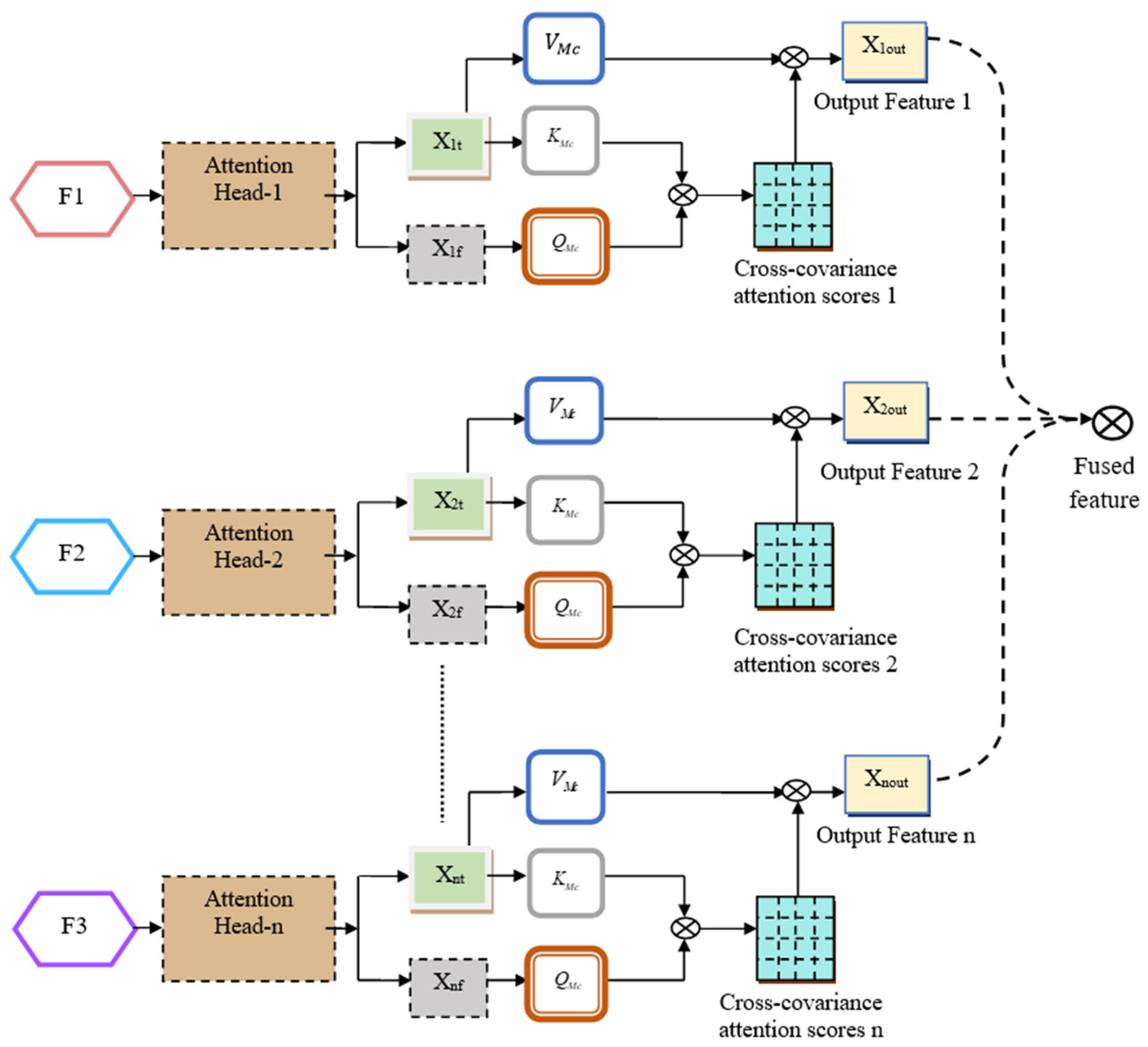
Further, the structure allows for the integration of each input element to improve the lower-level feature map. CCA [33] is the kind of attention module that highlights the meaningful feature from the input. It is the kind of transposed mechanism that works across the features channel and provides linear complexity in regard to token length, and ensures effective input processing. The attention weight is computed in terms of cross cross-covariance matrix among the keys and queries to determine across feature dimensions. The efficient processing allowed by this layer fixes the channel number and leads to more robust performance. An illustration of MCF is depicted in Figure 2.

5.2. Bi-GRU

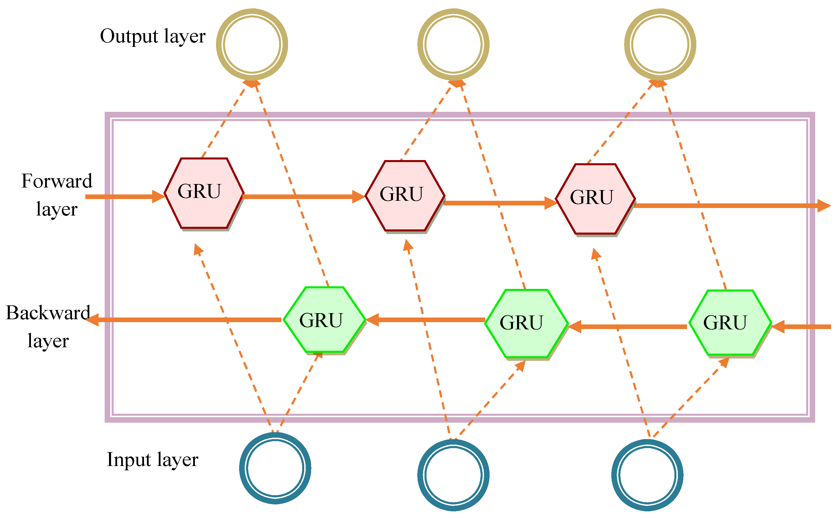
Bi-GRU [34] is the improved version of the GRU network that represents the variations. The structure is a combination of the two GRUs, operating in both forward and backward directions. The given input is processed in both directions simultaneously, and it is represented as j y G = j 1 G , j 2 G , j 3 G , j t G . The model can preserve both the future and past data based on its improvement. With the help of the reset and update gate, the input sequence is processed from left to right in the forward GRU. The hidden state is controlled based on the update gate in response to the added data. The inputs are considered using the sigmoid activation function while computing the update gate. The hidden state and reset gate are evaluated using Equations (16) and (17).
V t = σ z V . I t 1 , j t G
S t = σ z S . I t 1 , j t G
The terms z V and z S are the weight metrics of reset and the update gate. The candidate cell states are used to perform the new memory content based on the computation of the hidden state. The candidate’s weight is evaluated Equations (18) and (19).
I t = 1 V t × G t 1 + G t 1 × G ˜ t
G ˜ t = tanh z G . S t × I t 1 , j t G
The forward and backward computations are evaluated using Equations (20)–(22).
G t = G R U f r w j t G , G t 1
G t = G R U b c k j t G , G t 1
G t = G t G t
The concatenation of the forward and backward GRU obtains the output of Bi-GRU. The general structure of Bi-GRU is depicted in Figure 3.

5.3. Proposed MCF-DD-BiGRU for Estimation

This framework implemented the MCF-DD-BiGRU to learn from extracted features and predict the tool condition for different machining processes. The main aim of designing the model is to monitor the tool wear value in real-time.
MCF-DD-BiGRU is constructed by incorporating the MCF into the baseline Bi-GRU, which includes added dense and dilated layers.
Reasons for using DBiGRU: The decision to utilize the DBi-GRU instead of standard GRU is driven by the requirement to efficiently capture both complex temporal dynamics and long-term dependencies in the sequential data attained from the milling task. Although the standard GRU is effective in modeling temporal relations, it often struggles to retain long-range dependencies when handling lengthy time-series sensor data, such as current and vibration signals, which exhibit gradual changes in tool wear patterns. The inclusion of dilated connections enables the technique to skip specific time sequences during the information flow, thus expanding the receptive field without increasing computational expenses or network depth. This enables the DBi-GRU to capture broader contextual data over longer sequences, which is significant for precisely tracking the gradual degradation trends of the tool. In addition, the bi-directional design enhances the technique’s ability to learn from both future and past temporal contexts simultaneously, ensuring that each prediction encompasses the entire temporal scope of the signal rather than just previous time sequences. This is highly significant for tool-life validation, where the future signal behavior can offer significant cues about the present state of wear. Thus, the integration of dilation and bi-directionality enables the designed DBi-GRU to outperform the existing GRU by providing a detailed temporal representation, enhanced feature learning effectiveness, and higher prediction accuracy, most importantly in the scenarios with non-linear, complex, and long-term temporal dependencies typical of real-world milling data.
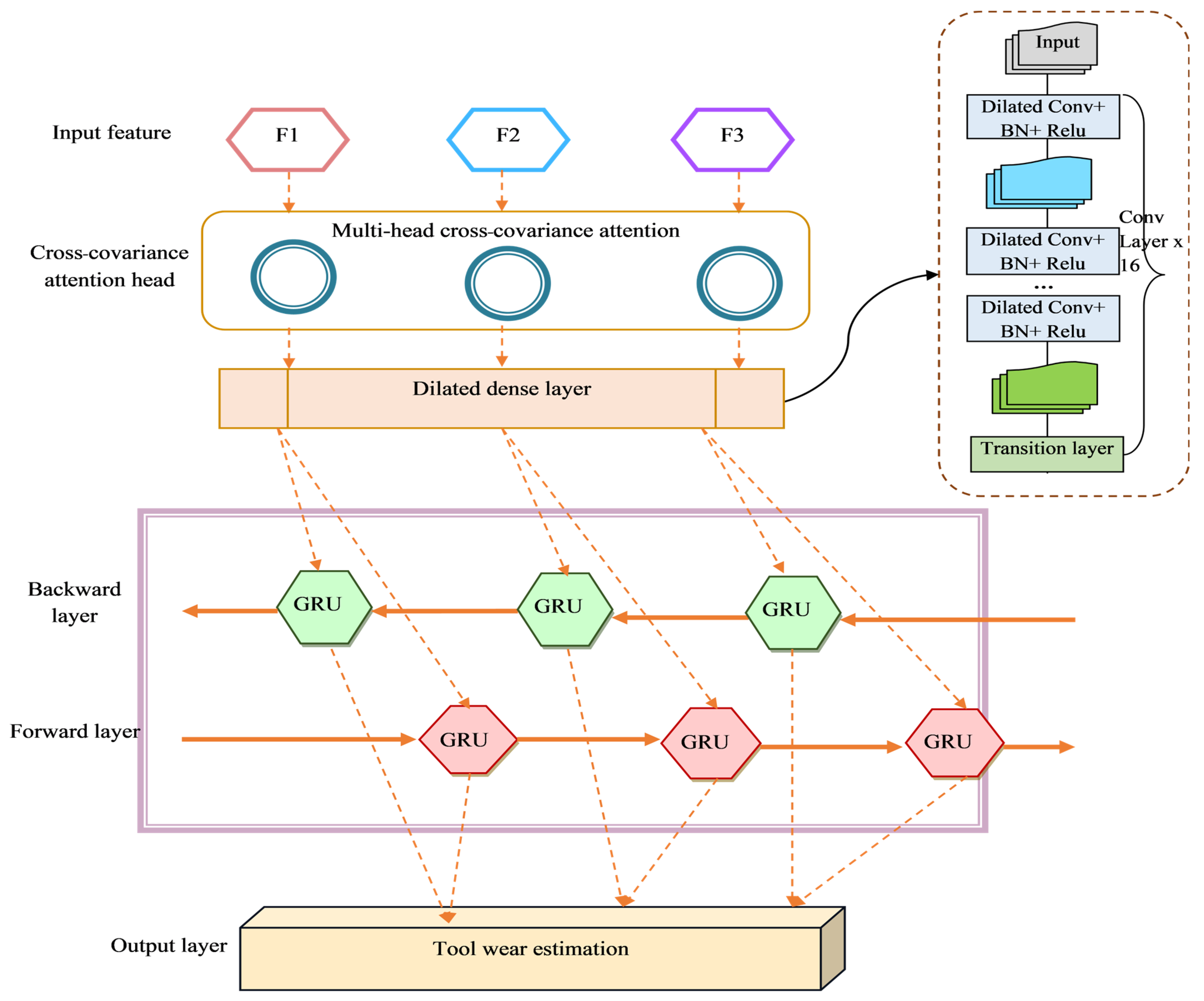
Here, the MCF performs feature fusion and sequence modeling, as attained by the DD-BiGRU. The extracted three feature sets from the previous process are given as input to the MCF-DD-BiGRU model. The three sets of representation, C t p F 1 , C t p F 2 , and C t p F 3 , are initially processed by each head in MCF. The data is jointly analyzed in this layer at different positions, ensuring that it focuses on various aspects of the input data simultaneously. The multi-head in the structure enables the network to focus on significant data simultaneously from different features and determine long-range dependencies between sensor modalities. The outcome from the parallel heads is linearly transformed to generate the final result, which tends to make the network capture different relationships. The model has the efficiency to fuse diverse data with different characteristics and adaptively learn the relationships and dependencies between them. The CCA operates across the feature channel, in conjunction with the token sequence. The cross-covariance matrix is computed by the key and query generated in each channel, which aggregates data from other channels. Here, the features are weighted and combined dynamically from different channels. The data-rich feature generated by this feature fusion process helps enhance further processing.
Other than the general concatenation, here the attention mechanism helps to focus on selective features, which are relevant to the prediction task. The features are further processed through the layers in DD-BiGRU. The construction of the Bi-GRU process features in both forward and backward directions to determine the previous and the future complex sequential pattern. DD [35] is the incorporation of the dilated convolution into the Densenet structure. The feature reuse encouraged by the propagation of the strengthened feature solves the vanishing-gradient issue, enabling a robust and deeper model. To perform better data flow and evaluate an effective receptive region based on the convolutional network. The typical dilation factor is considered in the structure with the base of the depth layer. In the transition layer, there are both the pooling layer and the convolution layer. The addition of a dilation layer helps in the effective evaluation of the multi-scale feature by placing the dilation in the transition layer.
The integration of efficient sequence modeling with the advanced feature fusion results in more robust and accurate predictions. The complex temporal relationships are learned effectively by the model during the wear progression. The result of the Bi-GRU estimates the level of current tool wear. Based on the results, the network can achieve high accuracy in processing real-time data, which makes it suitable for developing the tool condition monitoring system.
Exploration of a three-level feature extraction strategy (statistical, t-SNE, and FAE) combined with a multi-head cross-covariance attention mechanism and different recurrent architectures: The designed research work utilizes the DD-BiGRU model for estimating the tool life. To ensure its superiority, the exploration of a three-level feature extraction strategy (statistical, t-SNE, and FAE) combined with a multi-head cross-covariance attention mechanism and different recurrent architectures, such as the LSTM, GRU, and RNN, is given below.
Three-Level Feature Extraction + Multi-Head Attention + LSTM: This framework starts with the three-level feature extraction mechanism, including statistical features, t-SNE-based nonlinear manifold features, and FAE deep features, each capturing various characteristics of the milling process. These features are fused by employing the multi-head cross-covariance attention mechanism, which improves the representation by modeling the interdependencies between the feature groups. When an LSTM model executes this fused representation, the framework employs its memory cells to learn the long-term temporal patterns, but its complex gating structure often limits its capability to efficiently use all its temporal variations in the fused feature.
Three-Level Feature Extraction + Multi-Head Attention + GRU: Utilizing the same three-level feature extraction method, the statistical, t-SNE, and FAE-derived features are integrated via the multi-head cross-covariance attention module to produce the rich fused representation. This fused feature set is further given to the GRU model, which simplifies the learning tasks via the reduced gating strategy while still capturing the main temporal dependencies. Though GRU performs more effectively than LSTM and responds better to the attention-improved features, it still struggles to entirely model the intricate multi-scale temporal patterns embedded in the fused feature space.
Three-Level Feature Extraction + Multi-Head Attention + RNN: Likewise, the three-level features, such as statistical, t-SNE, and FAE, are fused by employing the multi-head cross-covariance attention mechanism before being subjected to the conventional RNN. While the RNN provides a baseline for the temporal sequence modeling, it lacks gating blocks and thus exhibits difficulty in retaining the long-term dependencies. As an outcome, its capability to learn from the rich fused features is limited, resulting in minimized prediction accuracy compared to highly advanced recurrent models.
Superiority of the designed DD-BiGRU approach: Although the LSTM, GRU, and RNN benefit from the attention-fused three-level features, these models do not entirely capture the complex temporal dynamics of the milling process. To resolve these problems, the designed DD-BiGRU combines the dilated connections, dense feature reuse and the bidirectional temporal learning. When integrated with the same multi-head attention, fused features, the designed DD-BiGRU attains tool-life prediction performance, demonstrating its superiority over LSTM, GRU and RNN in modeling complex, multiscale patterns in milling data.
Figure 4 represents the architectural view of the designed MCF-DD-BiGRU for tool-life estimation.

6. Results and Discussion

This section discusses the results obtained based on different performance metrics.

6.1. Experimental Setup

The designed tool wear estimation model was implemented in Python 3.10, and the determinations were carried out. Several performance measures were taken to evaluate the model’s performance in estimating tool wear. The comparative method used in the experimentation was LSTM [19], LSTM-AE [20], GAN-LSTM [22], and CNN-LSTM [5], respectively. The computer configuration is Intel Xeon®, CPU E52630, with 32 GB RAM. In the designed work, the training/testing splits were performed at the session level to eliminate the temporal or identity leakage. Each session appears in only some splits. Dataset 1 was split 80/20 into 1120 training sessions and 280 test sessions. Dataset 2 was split 80/20 into 774 training sessions and 193 test sessions. No session, subject, or tool instance appears in more than one split. Further, the initial experimental parameters of the model were epochs: 100; steps per epoch: 10; batch size: 32; optimizer: Adam; and hidden neuron count: 128. Table 2 presents the hyperparameter search ranges and the final picks for the designed model.

6.2. Evaluation Metrics

Accuracy, mean absolute error (MAE), mean absolute percentage error (MAPE), and mean squared error (MSE) were evaluated using Equations (23)–(26).
A c c u r a c y = T P + T N T P + T N + F P + F N
The terms T P and T N represent the true positive and true negative. F P and F N denote the false positive and false negative.
M A E = i = 1 z g i y i n
M A P E = 1 n i = 1 z g i y i g i
M S E = ( g i y i ) 2 n
Here, the predicted and observed values are indicated by the term a and b.
Root mean square error (RMSE), mean absolute scaled error (MASE), mean percentage error (MPE), and symmetric mean absolute percentage error (SMAPE) were calculated using Equations (27)–(30).
R M S E = i = 1 z g i y i 2 n
M A S E = 1 n i = 1 z y i g i y i
M P E = 1 n i = 1 z y i g i y i × 100
S M A P E = 100 % n i = 1 z g i y i g i + y i 2

6.3. K-Fold-Based Performance Analysis of MCF-DD-BiGRU for Tool-Life Estimation

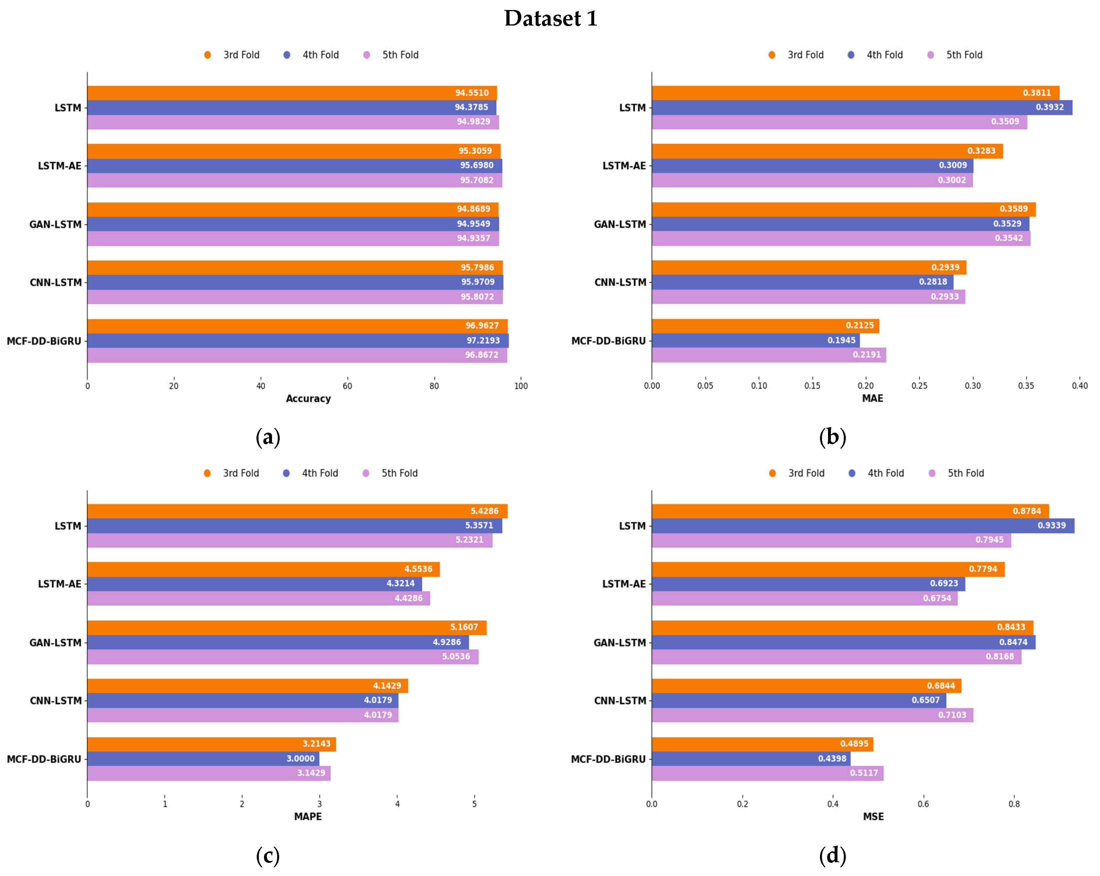
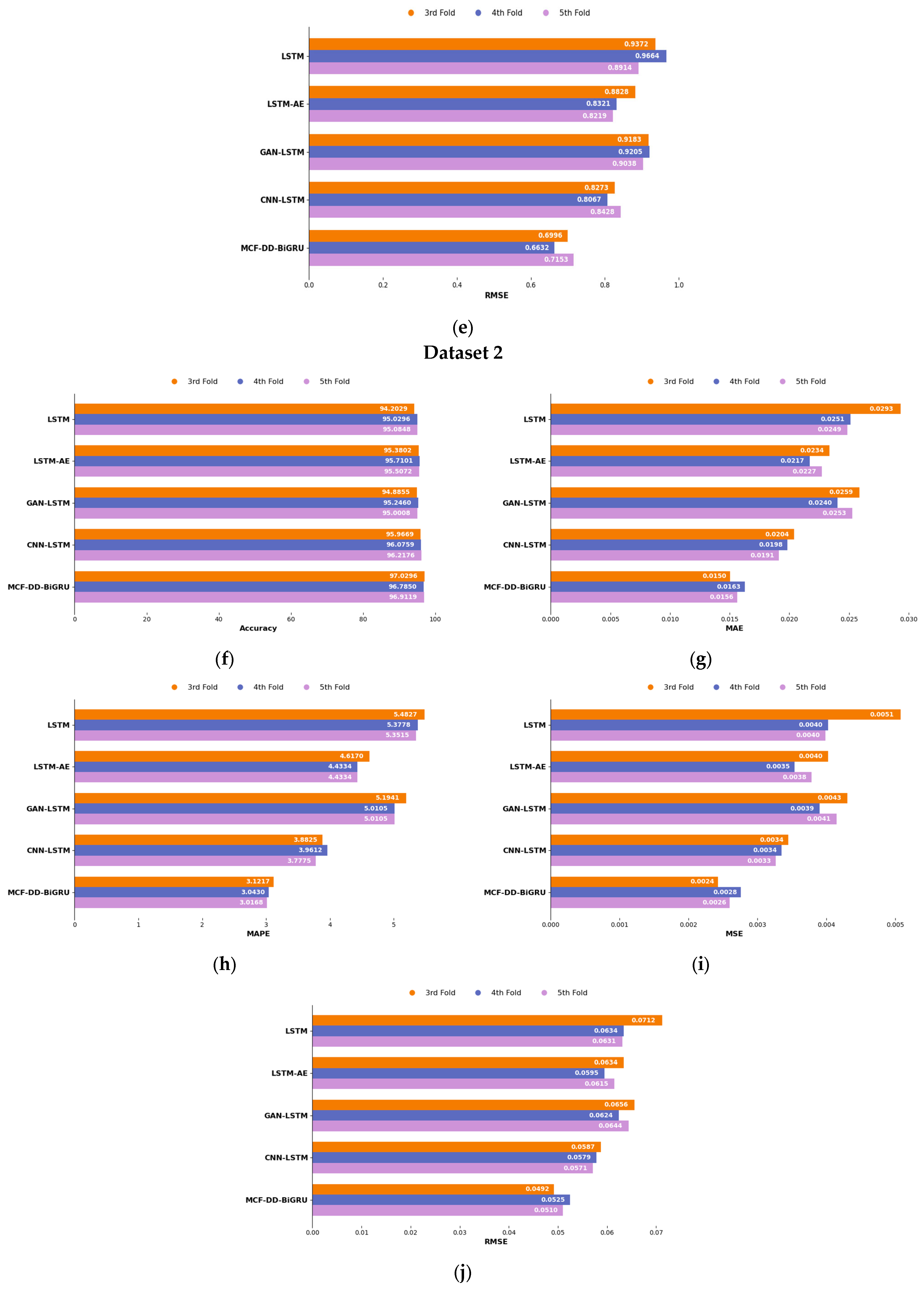
The K-fold method is considered a robust measure for evaluating the performance of the designed model for tool wear prediction. The reliable estimation of the network’s generalization is determined using this analysis. The comparison between MCF-DD-BiGRU and other traditional networks in terms of tool-life estimation is shown in Figure 5 for both datasets. In this study, the evaluation is performed utilizing k-fold cross-validation, where the experiments are performed with k = 3, 4, and 5 to guarantee the reliability and stability of the technique’s performance across distinct data partition settings. The folds are constructed by employing the run/tool-grouped strategy rather than random splitting, meaning that the entire samples originating from the same machining run or the same tool wear cycle are kept within the same fold. This eliminates the framework from encountering the data segments in the test set that are operationally or temporally correlated with the training set. To further prevent the temporal leakage, the sequence data are partitioned on the basis of their chronological order within each tool run, guaranteeing that the future time steps appear near in the training part of the fold. These precautions ensure that the validation reflects a realistic prediction scenario and that the designed framework is not unintentionally advanced by the data leakage across folds. From the analysis, the MCF-DD-BiGRU achieved better accuracy than the LSTM by 2.6%, the LSTM-AE by 1.4%, the GAN-LSTM by 2.1%, and the CNN-LSTM by 0.7%. From the outcome, the presented model MCF-DD-BiGRU provides more stable estimation in predicting tool wear than the other comparative models.

6.4. Performance Assessment of MCF-DD-BiGRU Based on Batch Size

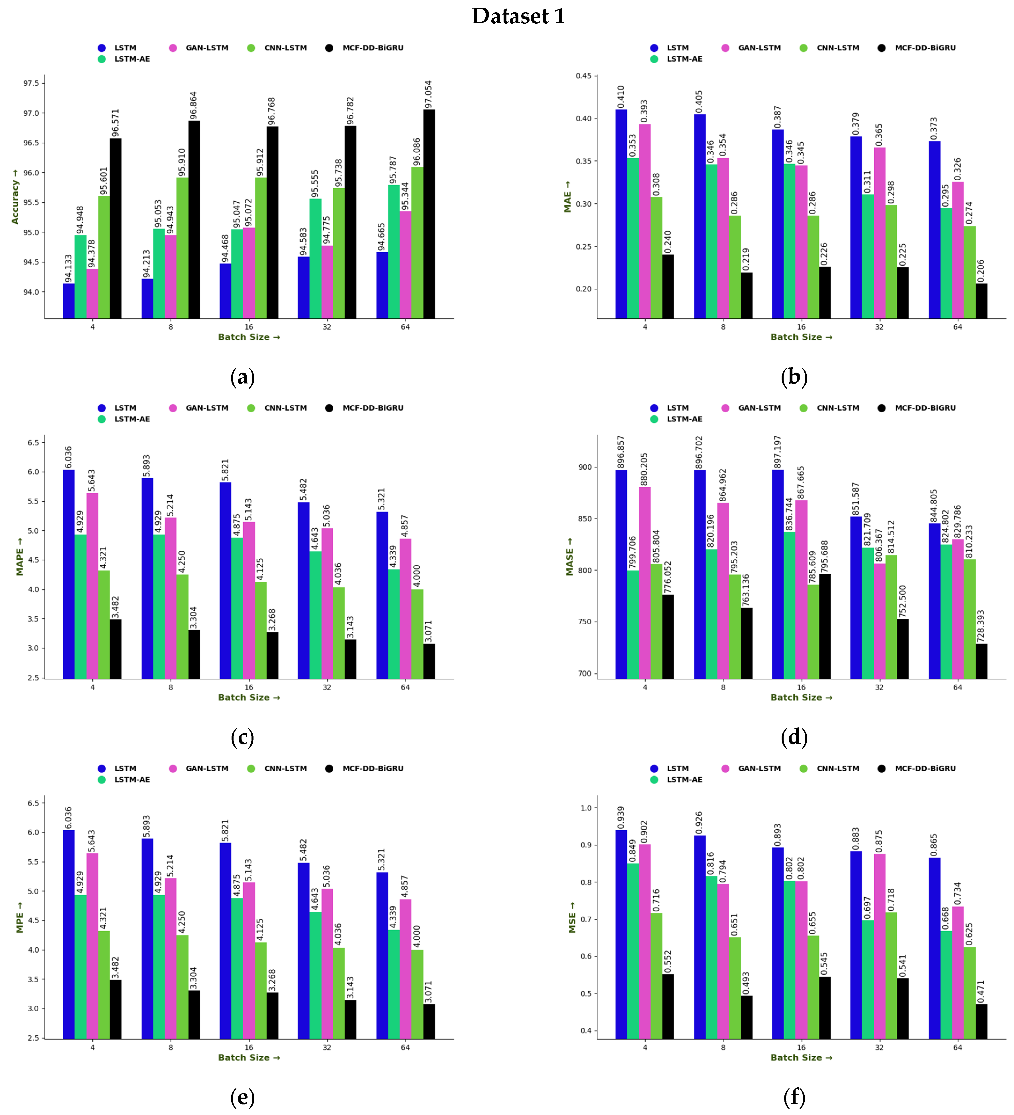
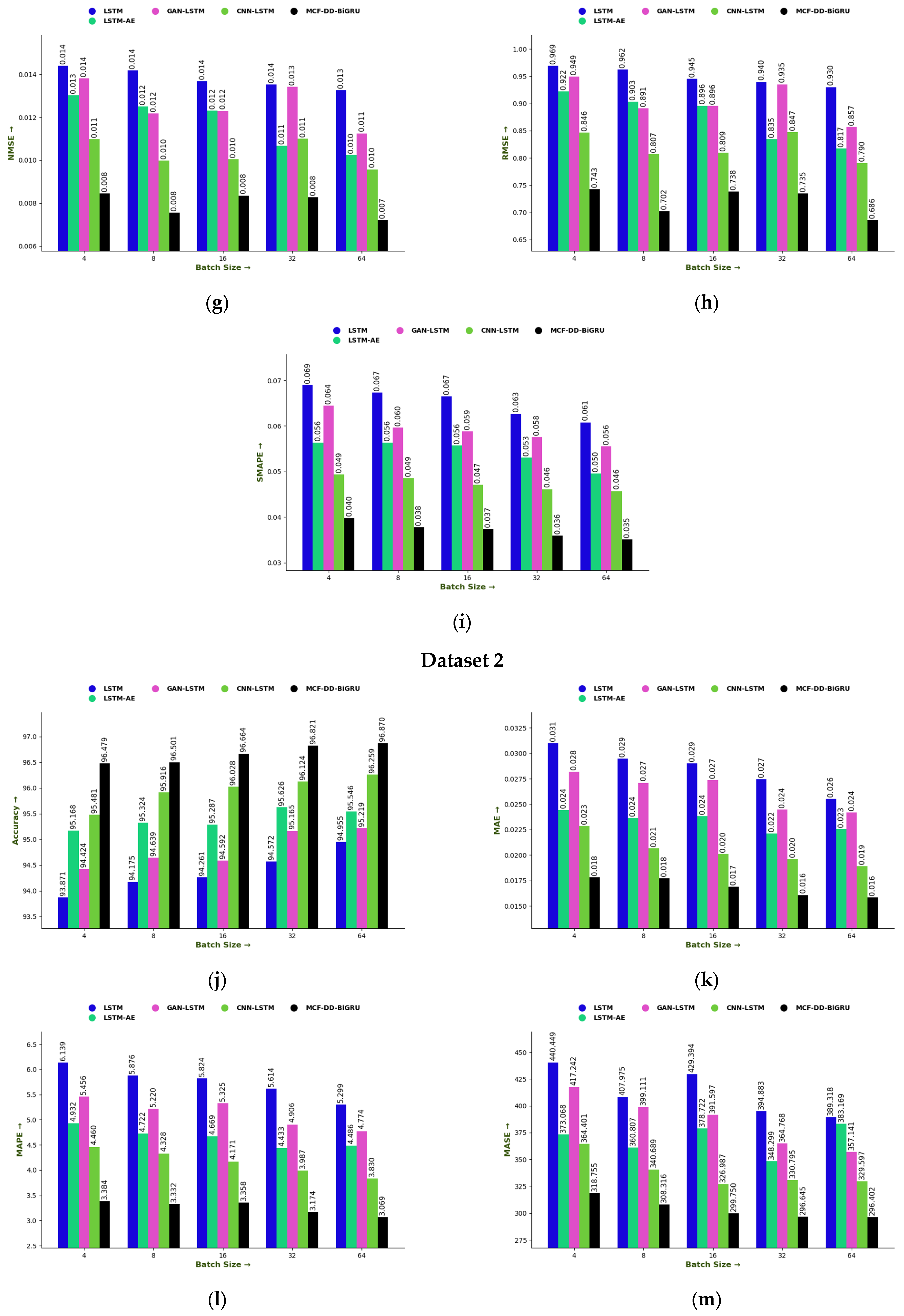
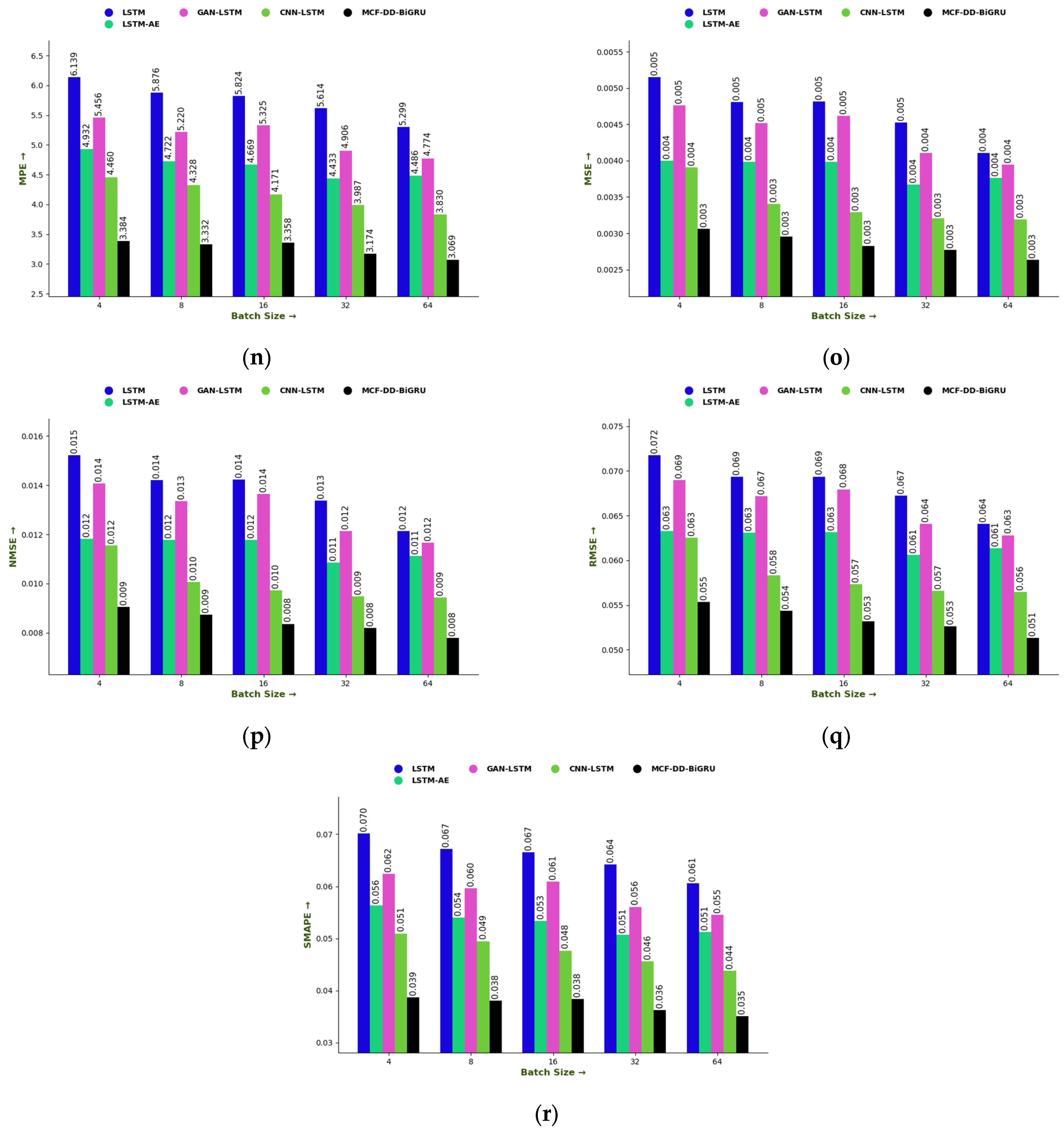
The model performance is analyzed through the determination of the batch size in this experiment. The designed MCF-DD-BiGRU for tool-life prediction is distinguished from other models, as shown in Figure 6. This analysis helps to evaluate the performance of the prediction model, where a smaller batch size provides more frequent generalization outcomes. Based on the graphical analysis, the MCF-DD-BiGRU achieved higher accuracy than the LSTM by 2.52%, the LSTM-AE by 1.68%, the GAN-LSTM by 2.27%, and the CNN-LSTM by 1.61%. The results show that the designed model provides a successful prediction for both datasets. This reveals the efficiency of the MCF-DD-BiGRU in predicting tool wear.

6.5. Epoch-Based Comparative Analysis for Designed MCF-DD-BiGRU

Some tracking model metrics are used in the epoch-based performance analysis to evaluate the model’s overfitting and underfitting based on the given dataset. The performance of the MCF-DD-BiGRU for tool-life prediction is compared to that of other conventional networks in Table 3 for the given dataset. The model’s parameters are updated during each epoch based on the measure of training data error, guiding the network to learn iteratively. From the comparison, the designed MCF-DD-BiGRU has a lower MPE value than the LSTM by 72.3%, the LSTM-AE by 39.6%, the GAN-LSTM by 55.7%, and the CNN-LSTM by 25.1%. According to the analysis, the proposed MCF-DD-BiGRU exhibits better prediction capability with fewer errors compared to other models.
The experimental results clearly demonstrate that the proposed MCF-DD-BiGRU framework is effective in predicting tool wear and estimating tool life during milling operations. The MCF-DD-BiGRU consistently achieved higher prediction accuracy and lower error rates than baseline models, including LSTM, LSTM-AE, GAN-LSTM, and CNN-LSTM, across various evaluation metrics, such as MPE, SMAPE, RMSE, and MASE. The two main reasons for these improvements are (i) the strong feature representation made possible by combining statistical, t-SNE, and fuzzy autoencoder-based deep features; and (ii) the cross-covariance attention mechanism, which makes the model better at finding complex relationships between different data sources.
The results in Table 3 and Figure 5 and Figure 6 demonstrate that the proposed method continues to perform better even when the batch sizes and epoch iterations are changed. This indicates its strong generalization capabilities. The multi-head attention fusion enables the network to utilize complementary details from different feature spaces, thereby improving temporal pattern recognition. This differs from traditional models that only utilize single-modality features. The addition of dilated dense layers to the Bi-GRU structure also enables efficient modeling of long-term dependencies without excessively increasing the number of parameters. This solves some of the scalability problems that LSTM-based architectures have.
These results are beneficial for real-time tool condition monitoring, where accurate and timely predictions of RUL can significantly cut down on downtime, make tool-change intervals more efficient, and boost machining productivity. The suggested method aligns with the general trend of utilizing AI-driven predictive maintenance strategies in smart manufacturing settings, resulting in lower operating costs and improved resource utilization.

6.6. Contributions of Features in Designed MCF-DD-BiGRU

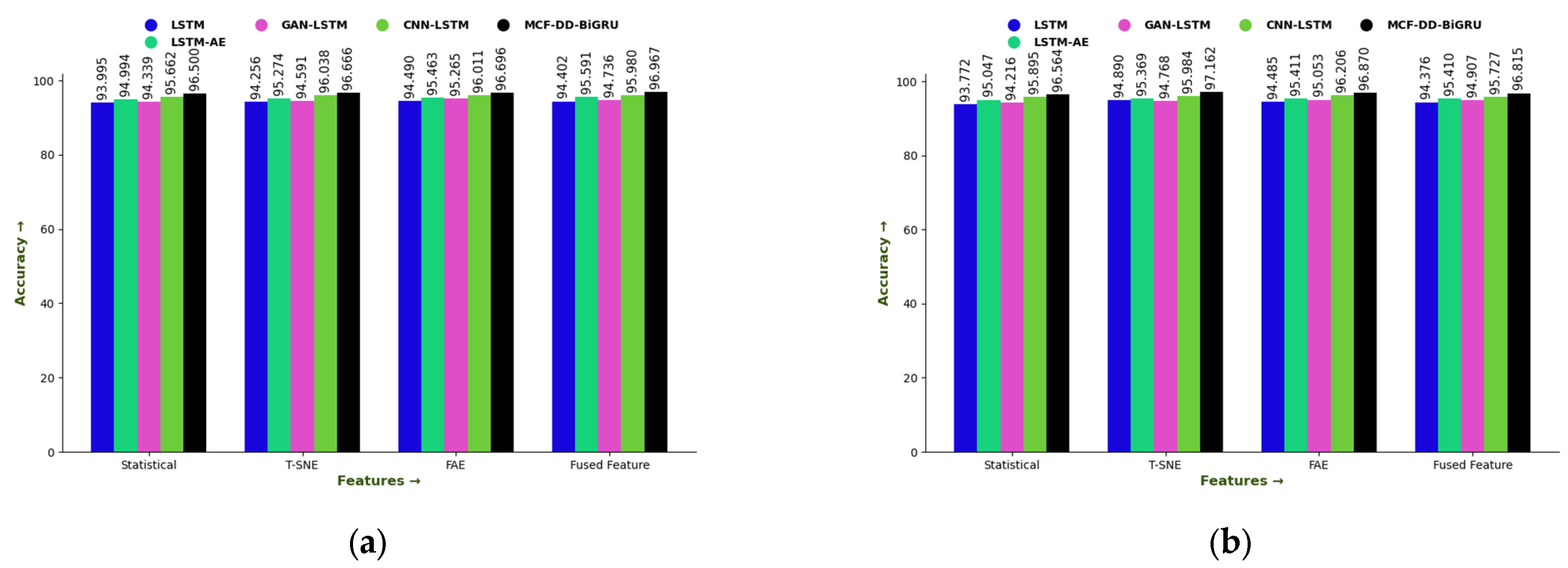
The implemented model utilizes three distinct features, including statistical, t-SNE, and FAE, to estimate tool life in the milling process. Figure 7 shows the accuracy analysis of these features. Although the statistical, t-SNE, and FAE features are extracted to capture various features of the milling process, the results show that the most significant contribution comes from the fused feature (accuracy: 96% for both datasets). These fused features are generated via the multi-head cross-variance attention method, which improves the interdependencies between all three feature types. As a result, no single feature type dominates individually; instead, the attention-driven fusion of all features provides the most substantial impact.

6.7. Ablation Study

The ablation study, presented in Table 4, was performed to validate the contribution of each component in the designed MCF-DD-BiGRU model, particularly the impact of eliminating the three-level feature extraction of the multi-head cross-covariance attention block. The results across both Dataset 1 and Dataset 2 demonstrate that the basic GRU, Bi-GRU, dilated Bi-GRU, dense Bi-GRU, and dilated dense Bi-GRU all significantly improve accuracy as additional architectural improvements are introduced. However, none of these models attains the performance of the designed MCF-DD-BiGRU model, which provides the highest accuracy, 96.52% on Dataset 1 and 96.49% on Dataset 2. This performance gain ensures that the combination of multi-head attention-based fused features, together with the DD-BiGRU, relatively improves temporal feature learning.

6.8. Computational Complexity Analysis

A detailed complexity analysis of the designed MCF-DD-BiGRU is presented in Table 5, which contrasts its training time, testing time, total computational time, and computational space with those of baseline models. Across both Dataset 1 and Dataset 2, the designed framework demonstrates lower training time (35.28 min for Dataset 1 and 37.65 min for Dataset 2) and testing time (10.53 min and 10.00 min). The minimization of execution time results in improved computation time, which is lower than that of all comparative approaches, indicating that the designed MCF-DD-BiGRU is not only accurate but also highly effective. Moreover, the designed model exhibits one of the smallest computational space footprints for both datasets (205 KB and 200 KB). These results clearly illustrate that, though MCF-DD-BiGRU includes multi-head attention, dense connections, and dilated BiGRU layers, its optimized model provides superior predictive performance while maintaining minimized computational overhead, making it both effective and computationally efficient compared to other high-complexity techniques.

6.9. Impact of Modifications to Key Parameters on Results

The performance of the designed MCF-DD-BiGRU technique is influenced by some primary parameters, and modifying them revealed their individual impacts on the computational efficiency and prediction accuracy. For the hidden size, increasing it improved the ability of the model to obtain the long-term temporal dependencies, but sizes larger than 128 offered negligible accuracy gains while increasing the computational cost. Refining the number of attention heads displayed, it was found that too few heads constrained the feature interaction learning, whereas too many heads provided redundancy without any improvement, making four heads optimal. The modifications in dilation rates affected the temporal receptive field: higher rates allowed the learning of long-term dependencies, but very large values can skip significant short-term patterns. Likewise, the depth of the dense blocks improves feature reuse up to a certain point; with one layer being enough for this process. The dropout rate tuning showed that lower rates caused overfitting, while higher rates (0.4) balanced stability and generalization. Adjusting the number of epochs and batch size also influenced performance: a small batch size slowed training, and too few epochs eliminated overall convergence, whereas the large batches and high epochs did not offer the additional accuracy measures. Finally, the k-fold setting ensured that the accuracy of the model is robust across distinct data splits. Thus, this analysis illustrates that careful tuning of each parameter is significant to attain a balanced trade-off among convergence stability, predictive accuracy, and computational efficiency, estimating the robustness of the designed MCF-DD-BiGRU approach.

7. Conclusions

This study proposed an improved deep learning framework named MCF-DD-BiGRU to make it easier to estimate tool wear and predict the remaining useful life of tools in milling processes. A three-level feature extraction strategy, statistical, t-SNE, and FAE, was used to extract diverse and informative feature sets from raw sensor data. A multi-head cross-covariance attention mechanism was utilized to combine these features. This made it easier to see how they were related and improved the quality of the representation. After that, the fused features were run through a dilated dense Bi-GRU network to find patterns over time and obtain a very accurate estimate of tool wear.
Two datasets were used to test the proposed model, and the results showed that it worked better than traditional LSTM, LSTM-AE, GAN-LSTM, and CNN-LSTM models. The MAE of the designed MCF-DD-BiGRU model was reduced by 62.5% compared to the LSTM, by 43.75% compared to the LSTM-AE, by 50% compared to the GAN-LSTM, and by 18.75% compared to the CNN-LSTM for the 64th batch size value in the second dataset. In addition, the model achieved an improvement of up to 3.4% in accuracy and demonstrated reduced prediction errors across multiple metrics, indicating its robustness and suitability for real-world applications.
This study provides a scalable, interpretable, and precise framework for estimating tool life, suitable for integration into contemporary predictive maintenance systems. The framework helps reduce unplanned downtime, improve machining accuracy, and make manufacturing operations more cost-effective by making it easier to predict tool wear.
Limitations and Future Research Directions: The developed MCF-DD-BiGRU framework shows great promise for predicting tool wear and tool life, but there are still some challenges that need to be explored further. One major problem with the model is that it is very sensitive to hyperparameter tuning. To obtain the best performance right now, one has to make manual adjustments, which can take a long time and may not always provide the optimal settings for all operating conditions. This shows that future work needs automated tuning strategies, such as advanced optimization techniques or reinforcement learning-based methods that can search for the best hyperparameters on their own.
Another limitation concerns the dependency on a specific set of publicly available datasets. While these datasets are well-established benchmarks, they may not fully capture the complexity of real industrial machining environments, where factors such as non-stationary noise, varying tool geometries, and mixed-material machining are often present. Therefore, future studies should focus on validating and enhancing the model’s robustness through transfer learning and domain adaptation strategies that allow better generalization across diverse operational settings.

Funding

This research was funded by the Ongoing Research Funding Program (ORF-2025-499), King Saud University, Riyadh, Saudi Arabia.

Data Availability Statement

The data presented in this study are openly available at https://www.kaggle.com/datasets/programmer3/milling-tool-wear-and-rul-dataset (accessed on 25 August 2025) and https://doi.org/10.1038/s41597-025-04923-y (accessed on 25 August 2025).

Acknowledgments

During the preparation of this manuscript, the author used ChatGPT 5 for the purposes of language corrections of some sections only. The authors have reviewed and edited the output and take full responsibility for the content of this publication.

Conflicts of Interest

The author declares no conflicts of interest.

Abbreviations

The following abbreviations are used in this manuscript:
t-SNEt-Distributed Stochastic Neighbor Embedding
MCF-DD-BiGRUMulti-head cross-covariance attention fusion-based dilated dense bi-directional gated recurrent unit
FAEFuzzy autoencoder
RULRemaining useful life
AIArtificial Intelligence
MLMachine learning
DBNDynamic Bayesian Network
MCFMulti-head cross-covariance attention fusion
Bi-GRUbi-directional gated recurrent unit
DDDilated dense
SVMSupport Vector Machine
KNNK-Nearest Neighbor
RNNRecurrent Neural Network
CNNConvolutional Neural Network
CCACross-Covariance Attention
MAEMean absolute error
MAPEMean absolute percentage error
MSEMean squared error
RMSERoot mean square error
MASEMean absolute scaled error
MPEMean percentage error
SMAPESymmetric mean absolute percentage error
KLKullback–Leibler divergence

References

  1. Wang, X.; Yan, J. Deep learning based multi-source heterogeneous information fusion framework for online monitoring of surface quality in milling process. Eng. Appl. Artif. Intell. 2024, 133, 108043. [Google Scholar] [CrossRef]
  2. Liu, R.; Tian, W. A novel simultaneous monitoring method for surface roughness and tool wear in milling process. Sci. Rep. 2025, 15, 8079. [Google Scholar] [CrossRef] [PubMed]
  3. Hojati, F.; Azarhoushang, B.; Daneshi, A.; Hajyaghaee Khiabani, R. Prediction of Machining Condition Using Time Series Imaging and Deep Learning in Slot Milling of Titanium Alloy. J. Manuf. Mater. Process. 2022, 6, 145. [Google Scholar] [CrossRef]
  4. Ahmed, M.; Kamal, K.; Ratlamwala, T.A.H.; Hussain, G.; Alqahtani, M.; Alkahtani, M.; Alatefi, M.; Alzabidi, A. Tool Health Monitoring of a Milling Process Using Acoustic Emissions and a ResNet Deep Learning Model. Sensors 2023, 23, 3084. [Google Scholar] [CrossRef]
  5. Bhandari, B.; Park, G. Non-contact surface roughness evaluation of milling surface using CNN-deep learning models. Int. J. Comput. Integr. Manuf. 2024, 37, 423–437. [Google Scholar] [CrossRef]
  6. Umar, M.; Siddique, M.F.; Ullah, N.; Kim, J.-M. Milling Machine Fault Diagnosis Using Acoustic Emission and Hybrid Deep Learning with Feature Optimization. Appl. Sci. 2024, 14, 10404. [Google Scholar] [CrossRef]
  7. Karabacak, Y.E. Deep learning-based CNC milling tool wear stage estimation with multi-signal analysis. Eksploat. I Niezawodn. Maint. Reliab. 2023, 25, 168082. [Google Scholar] [CrossRef]
  8. Farhani, G.; Kurukuri, S.; Myers, R.; Santos, N.; Tauhiduzzaman, M. Unlocking Dual Utility: 1D-CNN for Milling Tool Health Assessment and Experimental Optimization. IEEE Access 2024, 12, 105096–105107. [Google Scholar] [CrossRef]
  9. Hu, N.; Liu, Z.; Jiang, S.; Li, Q.; Zhong, S.; Chen, B. Remaining Useful Life Prediction of Milling Tool Based on Pyramid CNN. Shock Vib. 2023, 2023, 1830694. [Google Scholar] [CrossRef]
  10. Sayyad, S.; Kumar, S.; Bongale, A.; Kotecha, K.; Abraham, A. Remaining Useful-Life Prediction of the Milling Cutting Tool Using Time–Frequency-Based Features and Deep Learning Models. Sensors 2023, 23, 5659. [Google Scholar] [CrossRef]
  11. Zhu, M.; Zhang, J.; Bu, L.; Nie, S.; Bai, Y.; Zhao, Y.; Mei, N. Methodology and Experimental Verification for Predicting the Remaining Useful Life of Milling Cutters Based on Hybrid CNN-LSTM-Attention-PSA. Machines 2024, 12, 752. [Google Scholar] [CrossRef]
  12. Abidi, M.H.; Alkhalefah, H.; Umer, U. Fuzzy harmony search based optimal control strategy for wireless cyber physical system with industry 4.0. J. Intell. Manuf. 2022, 33, 1795–1812. [Google Scholar] [CrossRef]
  13. Abidi, M.H.; Alkhalefah, H.; Umer, U.; Mohammed, M.K. Blockchain-based secure information sharing for supply chain management: Optimization assisted data sanitization process. Int. J. Intell. Syst. 2021, 36, 260–290. [Google Scholar] [CrossRef]
  14. Abidi, M.H. Multimodal data-based human motion intention prediction using adaptive hybrid deep learning network for movement challenged person. Sci. Rep. 2024, 14, 30633. [Google Scholar] [CrossRef] [PubMed]
  15. Cen, Z.; Hu, S.; Hou, Y.; Chen, Z.; Ke, Y. Remaining useful life prediction of machinery based on improved Sample Convolution and Interaction Network. Eng. Appl. Artif. Intell. 2024, 135, 108813. [Google Scholar] [CrossRef]
  16. Abidi, M.H.; Mohammed, M.K.; Alkhalefah, H. Predictive Maintenance Planning for Industry 4.0 Using Machine Learning for Sustainable Manufacturing. Sustainability 2022, 14, 3387. [Google Scholar] [CrossRef]
  17. Danish, M.; Gupta, M.K.; Irfan, S.A.; Ghazali, S.M.; Rathore, M.F.; Krolczyk, G.M.; Alsaady, A. Machine learning models for prediction and classification of tool wear in sustainable milling of additively manufactured 316 stainless steel. Results Eng. 2024, 22, 102015. [Google Scholar] [CrossRef]
  18. Omole, S.; Dogan, H.; Lunt, A.J.G.; Kirk, S.; Shokrani, A. Using machine learning for cutting tool condition monitoring and prediction during machining of tungsten. Int. J. Comput. Integr. Manuf. 2024, 37, 747–771. [Google Scholar] [CrossRef]
  19. Khan, F.; Kamal, K.; Ratlamwala, T.A.H.; Alkahtani, M.; Almatani, M.; Mathavan, S. Tool Health Classification in Metallic Milling Process Using Acoustic Emission and Long Short-Term Memory Networks: A Deep Learning Approach. IEEE Access 2023, 11, 126611–126633. [Google Scholar] [CrossRef]
  20. Elminir, H.K.; El-Brawany, M.A.; Ibrahim, D.A.; Elattar, H.M.; Ramadan, E.A. An efficient deep learning prognostic model for remaining useful life estimation of high speed CNC milling machine cutters. Results Eng. 2024, 24, 103420. [Google Scholar] [CrossRef]
  21. Che, Z.; Peng, C.; Liao, T.W.; Wang, J. Improving milling tool wear prediction through a hybrid NCA-SMA-GRU deep learning model. Expert Syst. Appl. 2024, 255, 124556. [Google Scholar] [CrossRef]
  22. Shah, M.; Vakharia, V.; Chaudhari, R.; Vora, J.; Pimenov, D.Y.; Giasin, K. Tool wear prediction in face milling of stainless steel using singular generative adversarial network and LSTM deep learning models. Int. J. Adv. Manuf. Technol. 2022, 121, 723–736. [Google Scholar] [CrossRef]
  23. Wang, S.; Yu, Z.; Xu, G.; Zhao, F. Research on Tool Remaining Life Prediction Method Based on CNN-LSTM-PSO. IEEE Access 2023, 11, 80448–80464. [Google Scholar] [CrossRef]
  24. Kamat, P.; Kumar, S.; Kotecha, K. DeepTool: A deep learning framework for tool wear onset detection and remaining useful life prediction. MethodsX 2024, 13, 102965. [Google Scholar] [CrossRef] [PubMed]
  25. Li, X.; Liu, X.; Yue, C.; Wang, L.; Liang, S.Y. Data-model linkage prediction of tool remaining useful life based on deep feature fusion and Wiener process. J. Manuf. Syst. 2024, 73, 19–38. [Google Scholar] [CrossRef]
  26. Kaliyannan, D.; Thangamuthu, M.; Pradeep, P.; Gnansekaran, S.; Rakkiyannan, J.; Pramanik, A. Tool Condition Monitoring in the Milling Process Using Deep Learning and Reinforcement Learning. J. Sens. Actuator Netw. 2024, 13, 42. [Google Scholar] [CrossRef]
  27. Milling Tool Wear and RUL Dataset; Kaggle: San Francisco, CA, USA, 2025. Available online: https://www.kaggle.com/datasets/programmer3/milling-tool-wear-and-rul-dataset (accessed on 21 November 2025).
  28. Piecuch, G.; Żabiński, T. A new open dataset from a milling process—Data for classification and estimation of tool life. Sci. Data 2025, 12, 650. [Google Scholar] [CrossRef]
  29. Kanimozhi, M.; Roselin, R. Statistical Feature Extraction and Classification using Machine Learning Techniques in Brain-Computer Interface. Int. J. Innov. Technol. Explor. Eng. 2020, 9, 1754–1758. [Google Scholar] [CrossRef]
  30. Alalayah, K.M.; Senan, E.M.; Atlam, H.F.; Ahmed, I.A.; Shatnawi, H.S.A. Effective Early Detection of Epileptic Seizures through EEG Signals Using Classification Algorithms Based on t-Distributed Stochastic Neighbor Embedding and K-Means. Diagnostics 2023, 13, 1957. [Google Scholar] [CrossRef]
  31. Yang, W.; Wang, H.; Zhang, Y.; Liu, Z.; Li, T. Self-supervised Discriminative Representation Learning by Fuzzy Autoencoder. ACM Trans. Intell. Syst. Technol. 2022, 14, 11. [Google Scholar] [CrossRef]
  32. Voita, E.; Talbot, D.; Moiseev, F.; Sennrich, R.; Titov, I. Analyzing Multi-Head Self-Attention: Specialized Heads Do the Heavy Lifting, the Rest Can Be Pruned. In Proceedings of the 57th Annual Meeting of the Association for Computational Linguistics, Florence, Italy, 28 July–2 August 2019; pp. 5797–5808. [Google Scholar]
  33. Sarker, M.M.K.; Singh, V.K.; Alsharid, M.; Hernandez-Cruz, N.; Papageorghiou, A.T.; Noble, J.A. COMFormer: Classification of Maternal-Fetal and Brain Anatomy Using a Residual Cross-Covariance Attention Guided Transformer in Ultrasound. IEEE Trans. Ultrason. Ferroelectr. Freq. Control 2023, 70, 1417–1427. [Google Scholar] [CrossRef]
  34. Xu, H.; Zhang, A.; Xu, X.; Li, P.; Ji, Y. Prediction of Particulate Concentration Based on Correlation Analysis and a Bi-GRU Model. Int. J. Environ. Res. Public Health 2022, 19, 13266. [Google Scholar] [CrossRef]
  35. Srinivasulu, M.; Maiti, S. RNDDNet: A residual nested dilated DenseNet based deep-learning model for chilli plant disease classification. Eng. Res. Express 2024, 6, 035204. [Google Scholar] [CrossRef]
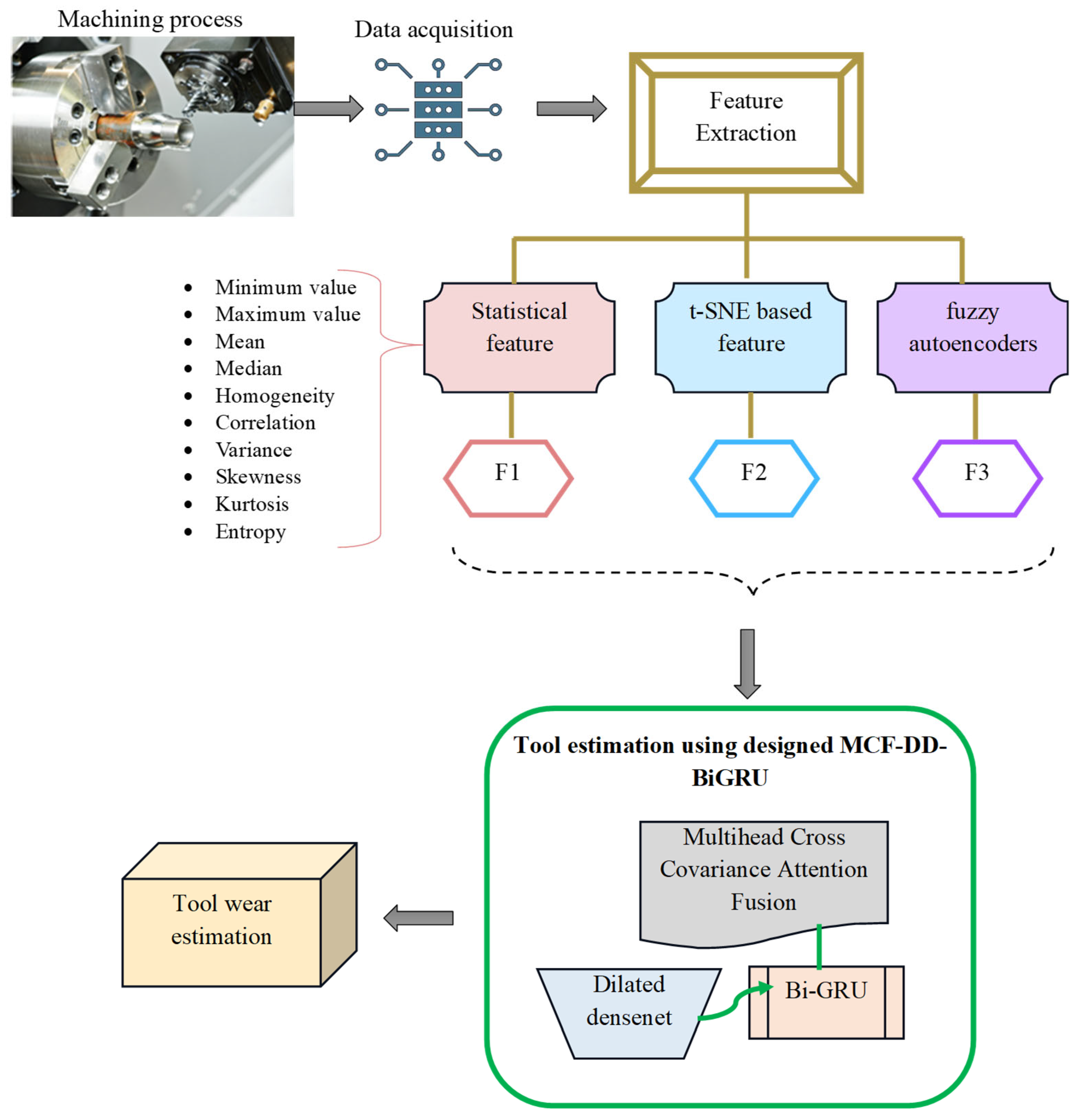
Figure 1. Architectural view of the implemented tool-life prediction model in the milling process.
Mathematics 13 03798 g001
Figure 2. Diagram structure of multi-head cross-covariance attention fusion.
Mathematics 13 03798 g002
Figure 3. Illustration of Bi-GRU.
Mathematics 13 03798 g003
Figure 4. Pictorial representation of MCF-DD-BiGRU for tool-life estimation.
Mathematics 13 03798 g004
Figure 5. K-fold-based performance analysis of MCF-DD-BiGRU for predicting tool wear compared with other methods regarding “(a,f) Accuracy, (b,g) MAE, (c,h) MAPE, (d,i) MSE, and (e,j) RMSE”.
Mathematics 13 03798 g005aMathematics 13 03798 g005b
Figure 6. Performance analysis of the MCF-DD-BiGRU model for tool wear prediction compared with other networks in terms of “(a,j) Accuracy, (b,k) MAE, (c,l) MAPE, (d,m) MASE, (e,n) MPE, (f,o) MSE, (g,p) NMSE, (h,q) RMSE, (i,r) SMAPE”.
Mathematics 13 03798 g006aMathematics 13 03798 g006bMathematics 13 03798 g006c
Figure 7. Contributions of features in the designed MCF-DD-BiGRU-based tool wear prediction compared with other networks in terms of accuracy for (a) Dataset 1 and (b) Dataset 2.
Mathematics 13 03798 g007
Table 1. Features and challenges of the existing tool-life prediction models using deep learning.
Author [Citation]MethodologyFeaturesChallenges
Khan et al. [19]LSTM
  • It efficiently preserves important details for a long time.
  • Variable time series are effectively handled by this approach.
Memory consumption is high.
Elminir et al. [20]LSTM-AE
  • It efficiently retrieves dynamic features by handling non-linear time series data.
It considers redundant data, which leads to high processing time.
The computational complexity of the model is high when dealing with long data sequences.
Che et al. [21]NCA-SMA-GRU
  • It retains and filters the most relevant features.
  • Interpretability of the model is high.
The modeling time is high.
Shah et al. [22]GAN and LSTM
  • It precisely identifies wavelet functions to generate feature vectors for precise tool-life estimation.
Computationally expensive, and it has training instability issues.
Wang et al. [23]CNN-LSTM-PSO
  • It uses a multi-channel feature fusion mechanism to improve the accuracy of tool wear prediction.
  • It helps in managing the spatial continuity of features.
The training time of the model is high.
Kamat et al. [24]DeepTool
  • It extracts useful features from the sensor signals to accurately predict the lifetime of tools.
It suffers from overfitting issues.
Li et al. [25]CSBLSTM-TSAM
  • It is capable of mining the temporal dependence of signal features.
  • This technique solves particle degradation issues.
Predicting the lifetime of machines with curved parts is complex.
The robustness of the model is affected by changing the parameters of the milling machine.
Kaliyannan et al. [26]LSTM and FFNN
  • The learning process of the model is highly consistent, and it is capable of overcoming premature convergence issues.
It is ineffective in capturing time-based patterns.
Table 2. Hyperparameters search ranges and the final picks.
HyperparameterSearched Range/DefaultsFinal Pick(s)
Learning Rate (LR)0.0001, 0.001, 0.01, 0.10.01
Hidden Size (HN)[64, 128, 256]128
Number of Attention Heads[4, 8, 16]4
Dilation Rates[1, 2, 3, 4]4
Depth of Dense Blocks[1, 2, 3]1
Dropout Rate[0.1, 0.2, 0.3, 0.4]0.4
Early StoppingPatience: 10, Monitor: ‘val_loss’-
Table 3. Epoch-based comparative analysis of MCF-DD-BiGRU with other models for tool-life prediction.
EpochLSTM [19]LSTM-AE [20]GAN-LSTM [22]CNN-LSTM [23]MCF-DD-BiGRU
Dataset 1
MPE
106.1254.9642865.5357144.4464293.553571
205.9464294.9107145.3754.253.267857
305.7678574.6255.0892864.1428573.196429
405.6607144.55.0535714.0714293.160714
505.3392864.4821434.7857143.9642863.053571
605.2678574.4107144.8214293.9285713.107143
SMAPE
1075.6734696.3265315.0816334.061224
206.7959185.6122456.1428574.8571433.734694
306.5918375.2857145.8163274.7346943.653061
406.4693885.1428575.775514.6530613.612245
506.1020415.1224495.4693884.5306123.489796
606.0204085.0408165.5102044.4897963.55102
RMSE
1010.158689.3364479.200718.7280497.445795
209.8390338.5170139.4409568.508157.509238
309.9565368.5953029.7266988.3997186.96534
409.6220798.892819.0536668.3503087.148677
509.3110878.3144258.785617.5595847.398947
609.6124368.6925879.0577678.1952017.015632
MASE
10946.7651855.762862.3747799.7338777.4966
20896.9576816.0386900.5572806.3521764.6227
30862.6906851.9967862.5689821.9569773.2036
40926.3732823.3261833.5765794.319784.6413
50847.9551793.5111839.9428753.1057761.0283
60905.8937813.4717848.5818817.0405728.18
MAE
104.3353713.6301083.7327963.2182342.466241
204.1435313.2784853.788533.093332.388016
304.2243913.2118933.8035562.9830112.105449
403.9817893.2750683.5246962.9427792.210008
503.7148292.9909793.3124192.5428212.249609
603.803383.1747583.4407392.8097222.114432
MSE
1010.319878.7169248.4653067.6178835.543986
209.6806577.2539528.9131667.2388625.638866
309.9132617.3879229.4608657.0555274.851596
409.2584417.9082078.1968876.9727645.110358
508.6696356.9129677.7186955.714735.474442
609.2398927.5561068.2043146.7161324.921909
NMSE
101.5813591.3357321.2971761.1673220.849529
201.483411.1115551.3658031.1092430.864068
301.5190531.1320841.449731.0811490.743431
401.4187121.2118091.2560451.0684670.783083
501.3284861.0593041.1827690.8756930.838873
601.4158691.1578551.2571831.0291420.754206
Accuracy
1093.8019794.8101894.6633795.399196.47411
2094.0761595.3129594.5836995.5775996.58595
3093.9606495.4081594.562295.735396.98992
4094.3074695.3177694.9609595.7928296.84044
5094.6890595.7239195.2643696.3646396.78382
6094.5625395.4612695.0809195.9830596.97708
Dataset 2
MPE
106.3746074.800635.692554.2235053.462749
205.9548794.800635.4039874.3546693.331584
305.8499484.7481645.0629594.0136413.147954
405.7974824.6432324.8793283.830013.279119
505.3777544.4596014.6694653.9349423.043022
605.2728234.3022044.800633.8562433.016789
SMAPE
107.2852655.4864346.5057714.8268633.957428
206.8055765.4864346.1759864.9767653.807525
306.6856545.4264735.7862394.5870183.597662
406.6256935.3065515.5763754.3771553.747564
506.1460055.0966875.3365314.4970773.477739
606.0260834.9168045.4864344.4071353.447759
RMSE
107.4313446.6432526.8852935.7781845.069942
206.8886376.4826186.7991026.1427595.406138
307.0389076.4969486.3595375.7395875.232892
407.2077746.3956336.3322275.3821665.42488
507.0785386.3451496.1120875.7247415.02194
606.7338886.1195976.3617395.7608225.054418
MASE
10449.2075382.5456424.1658330.4695291.034
20420.022380.3023395.9337359.679301.1804
30410.6396382.0612381.0258327.0288292.1369
40421.7488380.1668378.3147301.1708311.6336
50410.4199364.2985370.3846325.5384276.8786
60398.2375358.1721375.7199333.3341282.7617
MAE
103.2771642.5355182.883232.0552181.606044
202.9194012.452752.7491242.2081571.709625
302.9735012.4873242.4630181.974111.636935
403.0654012.4225432.4076641.7851261.687677
502.8794112.3419712.3000871.9876041.546472
602.697692.2306252.3904331.9789931.538482
MSE
100.5522490.4413280.4740730.3338740.257043
200.4745330.4202430.4622780.3773350.292263
300.4954620.4221030.4044370.3294290.273832
400.519520.4090410.4009710.2896770.294293
500.5010570.4026090.3735760.3277270.252199
600.4534520.3744950.4047170.3318710.255471
NMSE
101.6324921.3046011.4013970.9869590.75984
201.4027591.2422741.3665311.1154330.863954
301.4646271.2477721.1955490.9738180.809468
401.5357431.2091591.1853030.8563090.869955
501.4811651.1901461.1043210.9687860.74552
601.3404421.1070371.1963770.9810370.755194
Accuracy
1093.5212294.9874194.395.9369496.82494
2094.2284995.1510494.5651395.6345996.62016
3094.1215495.0826995.1307496.0972996.76386
4093.9398695.2107695.2401796.470996.66355
5094.3075595.3700495.4528596.0706196.94271
6094.6668195.5901795.2742496.0876396.9585
Table 4. Ablation study of the designed MCF-DD-BiGRU.
TermsGRUBi-GRUDilated Bi-GRUDense Bi-GRUDilated DenseBi-GRUMCF-DD-BiGRU
Dataset 1
Accuracy (%)95.8396.0696.2396.1196.1996.52
Dataset 2
Accuracy (%)95.7995.9695.896.3396.4396.49
Table 5. Computational complexity analysis of the designed MCF-DD-BiGRU.
TermsLSTM-AE [19]NCA-SMA-GRU [19]CNN-LSTM-PSO [19]CSBLSTM-TSAM [19]MCF-DD-BiGRU
Dataset 1
Training Time43.6464996142.2982282241.4720251540.1836369435.28433801
Testing Time11.8645186611.9119813811.4977195911.4153946910.5320641
Computational Time55.5110182754.210209652.9697447451.5990316345.81640211
Computational Space224226216205205
Dataset 2
Training Time41.3671496842.0627265139.2845189138.6013193237.6526821
Testing Time11.5123674211.5016251611.4400228110.9098639710.0094979
Computational Time52.8795171153.5643516750.7245417249.5111832947.66218
Computational Space209211205202200
All the time parameters are in minutes, and the computational space is in kilobytes.
Disclaimer/Publisher’s Note: The statements, opinions and data contained in all publications are solely those of the individual author(s) and contributor(s) and not of MDPI and/or the editor(s). MDPI and/or the editor(s) disclaim responsibility for any injury to people or property resulting from any ideas, methods, instructions or products referred to in the content.