Abstract
We present PyRMLE (Python regularized maximum likelihood estimation), a Python module that implements regularized maximum likelihood estimation for the analysis of Random coefficient models. PyRMLE is simple to use and readily works with data formats that are typical to Random coefficient problems. The module makes use of Python’s scientific libraries NumPy and SciPy for computational efficiency. The main implementation of the algorithm is executed purely in Python code, which takes advantage of Python’s high-level features. The module has been applied successfully in numerical experiments and real data applications. We demonstrate an application of the package in consumer demand.
Keywords:
Python; random coefficients model; penalized maximum likelihood; regularization; adaptive estimation MSC:
62G05
1. Introduction
The random coefficients model is often used to model unobserved heterogeneity in a population, an important problem in econometrics and statistics. The model is given by
Here, are the regressors, and are the regression coefficients. It is assumed that , , are i.i.d. random variables with and being independent, and that and are observed while is unknown.
In this paper, we introduce an open source
Python module named PyRMLE (version 1.0) which implements regularized maximum likelihood estimation (RMLE) to nonparametrically estimate the density .
Nonparametric estimation of the random coefficients model was first established by [1] for a single regressor. Kernel methods for estimation were developed by [2,3]. Constrained least squares methods were developed by [4,5]. Further recent studies on this model include [6,7,8,9,10,11]. Regularized maximum likelihood methods have been considered for problems other than the random coefficients model in [12,13,14,15] among others. The method implemented by the PyRMLE module is the one developed in [16].
Python was chosen as the programming language mainly for the extensive scientific and computational libraries at its disposal, namely, NumPy, SciPy by [17,18]. The module takes advantage of the benefits of working with NumPy arrays in terms of the computational efficiency achieved by performing array-wise computation. Another advantage is that there are no software-imposed limits in terms of array size. The maximum array size in
Python
is solely determined by the amount of RAM available to the user, which allows the user’s flexibility to increase the computational complexity of the method to the level that their system allows. The module uses a trust-region constrained minimization algorithm developed by [19], which is implemented in SciPy.
The paper is organized as follows: Section 2 briefly describes the regularized maximum likelihood method developed in [16], Section 3 discusses the classes and functions available to the module, Section 4 discusses examples of the module’s usage for general cases, and Section 5 demonstrates the usefulness of the model in a real data application.
2. Regularized Maximum Likelihood
It is assumed that the random coefficients have a Lebesgue density . If the conditional density exists, the two densities are connected by the integral equation
Here, is the induced Lebesgue measure on the d-dimensional hyperplane . This connection allows us to employ maximum likelihood estimation to nonparametrically identify as seen in the following expression of the log-likelihood
Direct maximization of over all densities is not feasible due to ill-posedness and will lead to overfitting. We stabilize the problem by adding a penalty term and state the estimator as a minimization problem with negative log-likelihood
Here, is a constraint that ensures that is a probability density, is a regularization parameter that controls a bias–variance trade-off, and is a regularization functional. See [16] for further details. In principle, can be any convex lower semi-continuous functional. We implemented the most popular choices, which are
- Squared norm: .
- Sobolev Norm for :
- Entropy: .
Of course, other penalty terms are possible, e.g., higher-order Sobolev norms , Banach space norms , or total variation have been considered for other types of problems. However, these are often not suitable for density estimation problems like ours. We have chosen the three penalties above since they provide good options for obtaining either a smooth reconstruction with , a very mild smoothness assumptions with entropy, or a compromise with .
In addition to the regularization functional, a regularization parameter also needs to be chosen. In this module, we implement two methods of estimating : Lepskii’s Balancing principle and K-fold cross validation.
Remark
The linear random coefficient model is a regression model with a nonparametric component, but it is different from the standard nonparametric regression . When estimating the random coefficients model, we estimate a density that makes it possible to use a maximum likelihood approach without any distributional assumptions. We only need regularity assumptions for , as for most nonparametric methods. In contrast, a maximum likelihood approach for nonparametric regression requires distributional assumptions on , e.g., ∼. With an assumption like that, m can be estimated by penalized maximum likelihood as well. However, the likelihood functional will be quite different, and the constraint is not required.
3. Python Implementation
The PyRMLE module’s implementation of regularized maximum likelihood is limited to applications with up to two regressors for the random coefficients model with intercept and up to three regressors for a model without intercept. Hence, the model can estimate bivariate and trivariate random coefficient densities. For higher-dimensional estimation problems, the computational costs of a fully nonparametric likelihood maximization becomes prohibitive. Parametric or semi-parametric methods would be more feasible for these types of problems.
There are two main functions used to implement regularized maximum likelihood estimation using PyRMLE, namely, transmatrix() and rmle(). There are other sub-functions necessary to the implementation; these will be discussed under the appropriate subsections when relevant.
Note: For the three-dimensional implementation of the algorithm, we observe numerical instabilities in the optimization algorithm when all the random coefficients, , have an expectation of zero. This is unexpected as our formulation and implementation of the problem should not be sensitive to . A simple shift by some constant c is enough to remove the instability
Since we want the algorithm to be as robust as possible, we repeat the estimation with 10 different random shifts c∼, producing 10 approximations, say . Just averaging over all 10 approximations is not feasible. If only one suffers from the instability, it can significantly impact the average in a negative way. Hence, a simple k-means clustering algorithm on the distances of is applied instead, using sklearn.cluster.K-means(). Then, we pick the approximation, , that is closest to the centroid of the largest cluster as the solution. This is a robust estimator, since the numerical instability will effect only one or two of the approximations.
3.1. The transmatrix() Function
The purpose of the function transmatrix() is to construct the discrete version of the linear operator given by
The linear operator above describes the integral of over the hyperplanes parametrized by the sample points . The function makes use of a finite-volume method as a discrete analog in evaluating the integral. The function is used as follows:
| trans_matrix = transmatrix(sample,grid) |
The argument
sample
corresponds to the sample observations. The sample data should be in the following format:
In the case of a random coefficients model with intercept the first column would simply be .
The
grid argument is a class object generated by the
grid_set()
function. It has the following attributes and methods: {
scale, shifts, interval, dim, step, start, end, ks(), numgridpoints()}. The grid_set() function is used as follows:
| grid_beta = grid_set(num_grid_points=20,dim = 2) |
| print(grid_beta.interval) |
| [−5. −4.5 −4. −3.5 −3. −2.5 −2. −1.5 −1. −0.5 0. 0.5 1. 1.5 |
| 2. 2.5 3. 3.5 4. 4.5 5. ] |
| print(grid_beta.num_grid_points) |
| 20 |
The base grid that is generated by the
grid_set()
function is a symmetric grid that spans in each axis. The user inputs the number of grid points by passing an integer value to the function as num_grid_points. This specifies the step size of the grid as , where k is the number of grid points along each axis. Additionally, the user can change the range over which each axis is defined by supplying new axis ranges through the arguments B0_range, B1_range, B2_range, which are passed as lists or arrays that contain the end points of the new range (e.g., B0_range = [0,10]). This is especially useful if the user expects a random coefficient to be significantly larger or smaller than the other random coefficients.
| grid_beta_shifted = grid_set(num_grid_points = 20, \ |
| dim = 2, B0_range = [0,10]) |
| print(grid_beta_shifted.shifts) |
| [−5,0,0] |
The output of the transmatrix() function is the ‘tmatrix’ class object that has the following attributes and methods:
| Tmat: Returns a NumPy array that is produced by the function transmatrix_2d() or transmatrix_3d(). |
| grid: Returns the class grid_obj. |
| scaled_sample : Returns the scaled and shifted sample. |
| sample: Returns the original sample. |
| n(): Returns the number of sample observations. |
| m(): Returns the number of grid points is to be estimated over. |
3.1.1. transmatrix_2d()
The 2-dimensional implementation of this method works for the random coefficients model with a single regressor and random intercept
and the model with two regressors and no intercept
The function first initializes an -dimensional array of zeros, where n is the sample size and m is the number of grid points is to be estimated over. In this 1-dimensional case, the hyperplanes that is integrated over reduce to lines, which simplifies the problem. A finite-volume type method of estimation is employed to approximate the integral expression as seen in (4).
To implement this finite-volume method, the lines parametrized by the sample points given by Equations (5) or (6) are made to intersect with the grid. The length of each line segment that intersects with the grid is then calculated and stored in an object. The intersection points of these lines with the grid are retrieved and subsequently mapped to their respective array indices. These indices are used to map the length of the line segments to the appropriate entry in the initialized array, forming the discretized linear operator T. The algorithm is outlined as follows (Algorithm 1):
| Algorithm 1: transmatrix_2d() |
 |
The result of this function’s implementation is a large, sparse array, , where each row corresponds to a collection of all the lengths of the line segments intersecting the grid for a line parametrized by a sample point, i.e., each corresponds to the length of the line segment intersecting the grid at section . The resulting array is sparse because is equal to zero unless a line passes through a section of the grid. The algorithm’s implementation is illustrated in Figure 1.
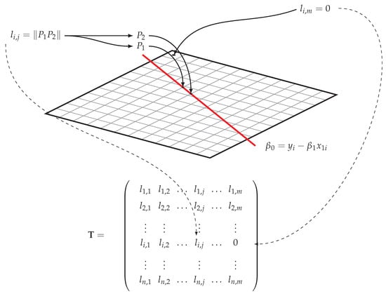
Figure 1.
Two-dimensional Transformation matrix algorithm.
The resulting array is then used to evaluate the log-likelihood functional
where is a -array or vector that serves as the discrete approximation of .
3.1.2. transmatrix_3d()
The implementation of the function for the 3-dimensional case works for problems with two regressors and a random intercept,
and the model with three regressors and no intercept.
It is significantly more complicated and computationally more expensive as the increased dimensionality introduces new problems.
Similar to the 2-dimensional implementation, a finite-volume type approach is used to create the discrete version of the linear operator T. In this higher-dimensional case, the hyperplanes parametrized by the sample observations are now 2-dimensional planes, and the grid that is estimated over comprises three axes and is, therefore, in the shape of a 3-dimensional cube. In this case, the intersection of the plane with the grid are characterized by a collection of points that define a polygon whose areas are used as the 2-dimensional analog of the line segments in the lower dimensional implementation of this finite-volume estimation process. The algorithm is outlined below. Figure 2 also illustrates the algorithm for a single cuboidal grid section (see also Algorithm 2).
| Algorithm 2: transmatrix_3d() |
 |
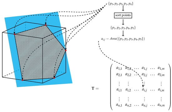
Figure 2.
Three-dimensional transformation matrix algorithm.
The resulting array is in the same form as the one obtained using the 2-dimensional implementation transmatrix_2d() and can be used in the following manner to evaluate the log-likelihood functional in (7):
where, in this case, each corresponds to the area of the polygonal intersection of the plane with the discrete estimation grid. Since we assume constant in each cube, the integral over the plane for observation i is given by . This explains why we can write the discretized operator evaluation conveniently as a matrix vector multiplication. The resulting product of this matrix and vector is an array. Applying an element-wise log-transformation, then taking the sum of this array results in the expression in (7).
It is important to note the computational performance of this algorithm. Matrix multiplication parallelizes the computation and eliminates the need to evaluate the log-likelihood functional sequentially for each sample point. However, the process of creating the transformation matrix scales linearly with the sample size n and exponentially with the dimensionality of the problem. Despite this, the function was written in a way that maximizes efficiency as much as possible by making use of Python’s parallel computation through array-wise computation when possible.
Solving for the transformation matrix, is only one of two steps in the process of estimating the density . The second step is the process of optimizing the regularized log-likelihood functional, the runtime of which scales multiplicatively with respect to the sample size n and the number of discretization points m. Therefore, choosing an appropriate sample size and level of discretization is an important consideration as both primarily determine the total cost of running the algorithm.
3.2. The rmle() Function
The rmle() function returns a class named ‘RMLEResult’. This class stores the solution to the optimization problem and metadata about the solution and the process of optimization. An instance of ‘RMLEResult’ has the following accessible attributes and methods:
| f: Returns a array containing all the grid-point estimates. It is necessary to reshape the solution before visual representation. |
| dim: Returns an integer representing the number of dimensions over which is estimated. |
| maxval(): Returns a list containing the maximum value of and its location. |
| mode(): Returns a list containing possible modes of the density and their locations. |
| ev(): Returns a tuple containing the expected value of each . |
| alpha: Returns a floating-point number specifying the regularization parameter used for estimation. |
| alpmth: Returns a string that specifies the method by which the regularization parameter was chosen. It can take on the following values: {‘Lepskii’, ‘CV’, ‘User’}. |
| T: Returns a class object that is created using the transmatrix() function. It contains attributes, methods, and subclasses that contain information about the transformation matrix and metadata about it. |
| Tmat: Returns an attribute of the subclass T but also accessible from the RMLEResult class. It returns the transformation matrix . |
| grid: Returns a class object that is created using the grid_set() function. It has attributes and methods that contain information about the grid is estimated over. |
| details: Returns a dictionary containing metadata about the minimization process. |
The function rmle() serves as a wrapper function for SciPy’s minimize function with ‘trust-const’ set as the minimization algorithm. The choice of this algorithm is crucial as it specializes in large-scale constrained minimization problems; for further details, we refer to [19]. The ability to handle large-scale problems is important because depending on the size of the sample, and level of discretization, the functional evaluations as well as the gradient evaluations could become exceedingly expensive, as it scales with both in a multiplicative manner (). The option to set constraints was also an important consideration. As in equation (2), there are two important constraints in estimating , namely, . These two constraints ensure the resulting solution satisfies the definition of a density.
Table 1 contains all the arguments for the function rmle(), followed by a short description of what they pertain to. More important arguments will be discussed in following subsections.

Table 1.
rmle() arguments.
3.2.1. Functionals and Regularization Terms
Recall the average log-likelihood functional to be minimized as in Equation (2). As specified in Section 2, the regularization terms implemented in this module are the Sobolev norm for , the squared norm, and Entropy. The module also includes an option for a functional that has no regularization term if the user wishes to produce a reconstruction of without any form of regularization. This option will often lead to overfitting and produce a highly unstable solution.
3.2.2. Sobolev Norm for
The functional incorporating the Sobolev norm for has the following form:
where indicates the squared norm. It is important to note that the choice of the regularization term would typically depend on knowledge about the true solution, as it imposes certain assumptions on . In the case of the penalty term, the solution has a square-integrable first derivative in addition to the assumptions of non-negativity and integrability imposed by the constraints of the minimization problem. The function is written as follows:
| def sobolev_norm_penal(f,a,tm_long,n,s): |
| tm=tm_long.reshape(n,len(f)) |
| f[f<0]=1e−6 |
| val=−np.sum(np.log(np.dot(tm,f)))/n |
| r=a*(s**2*np.sum(f**2)+s**2*norm_fprime(f,s)) |
| return val + r |
The function above returns the value of the discrete implementation of the functional in (10). Table 2 provides details on the arguments required for this function. The SciPy Optimize minimize function does not accept array arguments that are greater than one dimension. A necessary step is to unravel the transformation matrix, , into a one-dimensional array, which is passed to the function as tm_long and simply reshaped into the proper array dimensions. The term is calculated using NumPy’s matrix multiplication and sum functions, which are much faster alternatives than their non-Numpy counterparts. The regularization term is calculated in (10), with the function norm_fprime() computing for , where is treated as a total derivative.
Table 2.
sobolev_norm_penal() arguments.
The underlying minimization function is able to approximate the Jacobian of the functional being estimated using finite-difference methods, which necessitates a quasi-newton method of estimating the Hessian. Choosing to approximate the Jacobian, however, increases the computation time severely as it requires profusely more function evaluations, gradient evaluations, and consequently a lot more iterations, as it seems to converge to the solution more slowly. To this end, we opt to supply an explicit form for the Jacobian of the functional. The explicit form, as well as the function, are written as follows:
| def jac_sobolev_norm_penal(f,a,tm_long,n,s): |
| tm=tm_long.reshape(n,len(f)) |
| f[f<0]=1e−6 |
| denom=np.dot(tm,f) |
| temp=tm.T/denom |
| val=−np.sum(temp.T,axis=0)/n |
| r_prime=2a*(s**2*f−s**2*second_deriv(f,s)) |
| return val + r_prime |
The function has identical arguments to the functional being optimized, sobolev_norm_penal(). The function second_deriv() is used to solve for , and produces the Laplacian of f given by
The form of this Jacobian implies an additional smoothness assumption on the solution, as it requires to be second-order differentiable.
3.2.3. Squared Norm
The form of the functional that incorporates the squared norm as the regularization term is
The arguments for this function are identical to those listed in Table 2; likewise is true for the Jacobian associated with this regularization term. The Jacobian has the following form:
Choosing this regularization functional imposes less smoothness on the solution, as the only additional assumption in place is square-integrability. This leads to a typically less smooth reconstruction as compared with using the Sobolev norm for as the regularization functional. The functions in Python are coded similarly to the Sobolev norm for the regularization functional.
3.2.4. Entropy
The form of the functional that uses the entropy of the function has the following form:
For densities on a compact domain, the entropy is bounded by the norm and by the Sobolev norm. Since we only work on discretized bounded domains, the entropy implies weaker assumptions on the solution than the other two. The Jacobian has the following form:
3.2.5. Parameter Selection
Recall the minimization problem as in (2), where a constant controls the size of the effect of the regularization term. The module allows for the user to provide the value directly if the user has a general idea of the level of smoothing necessary for the solution, which is typically affected by the sample size, and the level of discretization of the grid is estimated over. If the user has no best-guess for the value of the regularization parameter alpha, the module has options to automatically select the parameter.
There are two methods implemented in the module for automated selection for , namely, Lepskii’s balancing principle and k-fold cross validation. The Lepskii method typically yields a less accurate result relative to k-fold cross validation; however, its advantage lies in significantly less computational cost.
3.2.6. Lepskii’s Balancing Principle
Lepskii’s principle is an adaptive form of estimation, which is popular for inverse problems [14,20,21,22,23,24]. The method works as follows: we compute for for and with some constants . We then select as the optimal parameter choice where
The algorithm is implemented in Python as follows (Algorithm 3):
| Algorithm 3: Lepskii’s Balancing Principle |
 |
The bulk of the computational cost of the Lepskii algorithm implementation can be broken down into two components: the fixed cost of generating and the variable cost of computing , as the number of values to be used depends on and also the sample size of the data. This implementation of Lepskii algorithm’s scales linearly in terms of runtime with the number of alpha values being tested, m.
3.2.7. K-Fold Cross Validation
Cross validation is another popular parameter choice rule as it optimizes for both training and testing performance. Here, we present a modified implementation of k-fold cross validation with a cost-function that is applicable to our problem. The modification we apply is an algorithm to lessen the computation time by reducing the number of values it needs to iterate through. We consider the loss function
where is a subsample of , which can be interpreted as the j-th fold that is left out in the current iteration, and is the estimate for using . The loss function can be interpreted as the negative of the likelihood that the subsample was drawn from the same distribution, , as . We aim to choose the that minimizes this loss function.
The modification we implemented changes the search method for the optimal value by reducing the number of values being tested. The algorithm involves separating the range of values into two sections, and . From there, two alpha values, and , are randomly selected from the respective sections and are used to compute for the corresponding loss function values, and . The section from which the value that produces the smaller was drawn from is kept, while the other is discarded. This is repeated until there is a sufficiently small range of values. Once this range of values is obtained, the loss function is evaluated over all the remaining values and the optimal is chosen as the one which minimizes . The complete algorithm is implemented as follows (Algorithm 4):
| Algorithm 4: Modified K-fold Cross Validation |
 |
The runtime of the unmodified version of k-fold cross validation scales linearly with the product , where k is the number of folds and m is the number of values being tested. Applying the modified version reduces the number of values being tested by a logarithmic factor, which is a significant reduction in computational cost.
4. Examples
This section presents three instructive examples of how the module can be used. The examples are (1) the random coefficients model with a single regressor and random intercept for the two-dimensional case, (2) the model with two regressors and random intercept for the three-dimensional case, and (3) the three-dimensional case with additional robustness. This section will also show how to plot the estimated density using the built-in plotting function plot_rmle(), which makes use of functions from the matplotlib library. It will also show how to plot the density without using the built-in function if the user wishes to explore different plotting options.
Example 1.
Two-Dimensional Case Single Regressor with Random Intercept
The first example is
We generate synthetic data using the function sim_sample(). This function draws the regressor ∼ and the random coefficients , from the bimodal multivariate normal mixture .
The general flow of the process of using the module can be broken down into five steps:
- Import the necessary modules and functions.
- Establish the dataset to be used (either real or simulated data).
- Specify the grid over which is to be estimated.
- Generate the transformation matrix .
- Run the rmle() function.
| from pyrmle import * |
| sample = sim_sample(n = 10000,d = 2) |
The program begins by importing the necessary functions from pyrmle.py, which contains the high-level functions that the user interacts with. The module pyrmle_funcs contains the underlying functions necessary for functions in the main module pyrmle to run. The next step is to define the sample to be used in creating the transformation matrix The sample has the same form as described in Section 3.1, where the sample has the form . In Python, it takes the shape of a 10,000 × 3 NumPy array as seen below.
| [[ 1. , −0.76765455, 2.10802347], |
| [ 1. , 1.51774991, −0.11337413], |
| …, |
| [ 1. , −1.80486996, −3.08120151]] |
The next step is to generate the grid on which is estimated. This is achieved using the grid_set() function, as discussed briefly in Section 3.1. In this example, we set the ranges of and to , which defines a two-dimensional grid spanning this range in each axis. The function creates an instance of the class grid_obj, which has attributes and methods enumerated and described in Section 3.1. When the grid class instance has been created, the user can proceed to generate an instance of the class tmatrix using the transmatrix() function.
| grid_beta = grid_set(num_grid_points = 40, dim = 2) |
| print(grid_beta.numgridpoints()) |
| T = transmatrix(sample, grid_beta) |
After the instance of the transformation matrix is produced, the user can then run the rmle() function. As stated in Section 3.2, the rmle() function has three essential arguments: {‘functional’,‘lpha’,‘tmat’}. We use Sobolev regularization with .
| result = rmle(sobolev,0.25,T) |
| print(result.ev()) |
| [−0.002865326246726808, −0.010416375635973668] |
| print(result.mode()[:2]) |
| [[0.39681799850755783, [−0.625, −0.375]], |
| [0.38831830923870914, [0.625, 0.375]]] |
| plot_rmle(result) |
| plot_rmle(result,plt_type=‘surface’) |
As stated in Section 3.2, the rmle() function generates an instance of class RMLEResult. This class has a number of useful and informative attributes and methods that describe the estimated density. The ev() method returns the expected value of each , while the mode() method returns possible maxima of the estimated density. The mode() method relies on a naive search method for maxima with no underlying statistical tests.
Figure 3 and Figure 4 show the contour and surface plots produced by the plot_rmle() function. It shows signs of oversmoothing as the two peaks are partially merged together. In the next reconstruction, shown in Figure 5 and Figure 6, we apply less regularization with . In addition, a large portion of the grid is essentially unused and the user could benefit in terms of computational costs by reducing the grid. This can be achieved by reducing the number of grid points and shrinking the range of each axis. We suggest that the user tries a relatively large range at first to ensure that the grid contains the support of , and then considers smaller grid ranges. Having a grid range that is too small has a negative effect on the estimate, as the optimization algorithm enforces the constraint that .
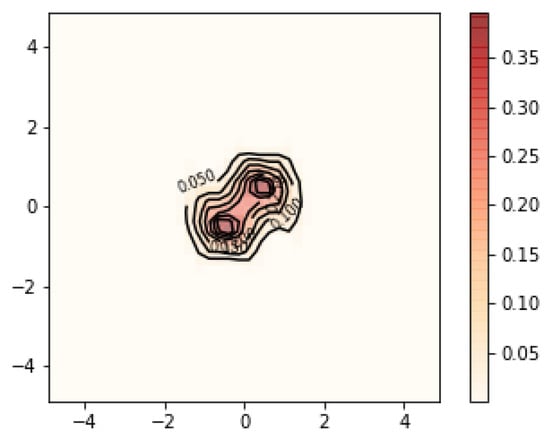
Figure 3.
contour plot with on a grid.
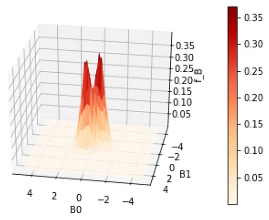
Figure 4.
surface plot with on a grid.
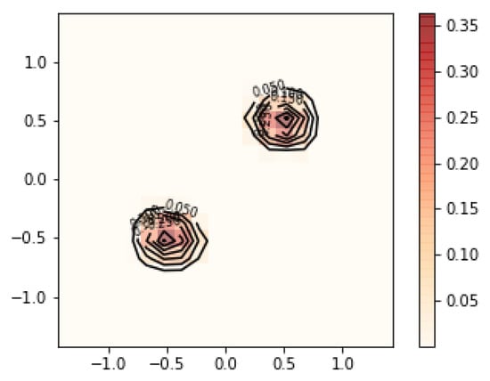
Figure 5.
contour plot with and a grid on a smaller domain.
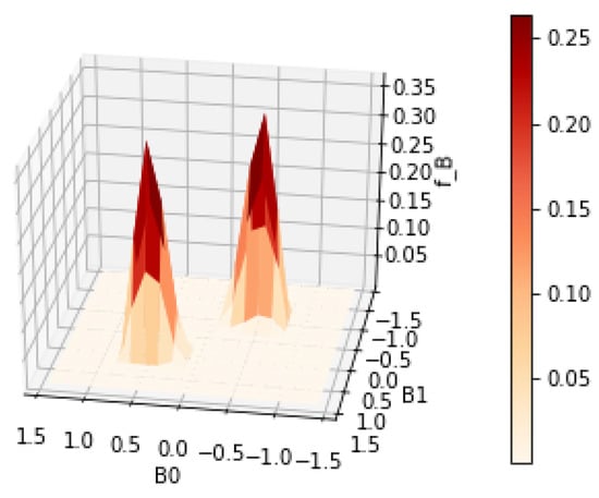
Figure 6.
surface plot with and a grid on a smaller domain.
| grid_beta_alt = grid_set(20,2,B0_range=[−1.5,1.5],\ |
| B1_range=[−1.5,1.5]) |
| print(grid_obj_ alt.numgridpoints) |
| 400 |
| T2 = transmatrix(sample, grid_beta_alt) |
| result2 = rmle(sobolev,0.15,T2) |
| print(result2.ev()) |
| [−0.004977073000670898, −0.003964663139211258] |
| print(result2.mode()[:2]) |
| [[0.3643228046077392, [0.5249999999999, 0.5249999999999]], |
| [0.3580092260598125, [-0.5249999999999, −0.5249999999999]]] |
| plot_rmle(result2) |
| plot_rmle(result2,plt_type=‘surface’) |
The smaller value for resulted in a reconstruction with less smoothness. The two peaks are well separated. There are no signs of overfitting yet. So we could continue to try smaller values of until becomes jagged, indicating overfitting. However, a better strategy is to choose by cross validation or Lepskii’s principle.
The reduction in the number of grid points resulted in a significant reduction in the runtime of the algorithm while achieving a better estimate for . The reduced computational cost of the algorithm makes an automatic parameter choice method such as cross validation more feasible.
| result_cv = rmle(sobolev,‘cv’,T2) |
| print(result_cv.alpha) |
| 0.07065193045869372 |
| print(result_cv.ev()) |
| [−0.004977073000670898, −0.003964663139211258] |
| print(result_cv.mode()[:2]) |
| [[0.3643228046077392, [0.5249999999999, 0.5249999999999]], |
| [0.3580092260598125, [−0.5249999999999, −0.5249999999999]]] |
| plot_rmle(result_cv) |
| plot_rmle(result,plt_type=‘surface’) |
Cross validation chose for this example. As shown in Figure 7 and Figure 8, the two modes become slightly sharper compared with the estimate with . Any smaller value of the regularization parameter will most likely lead to overfitting. The general workflow that we suggest when tuning the parameters to be used in estimation is as follows:
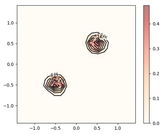
Figure 7.
contour plot with grid points using cross validation .
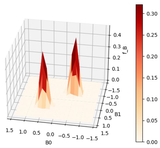
Figure 8.
surface plot with grid points using cross validation .
- Establish a relatively large grid range for estimation and generate the transformation matrix . This should be treated as an exploratory step in terms of analyzing the data.
- Set equal to the step size of the grid.
- Run the rmle() function.
- Plot using the plot_rmle() function and determine the necessary grid range.
- Limit the grid range and possibly also the number of grid points and generate a new matrix .
- Run the rmle() function with , and optionally employ one of the two automatic parameter selection methods {‘cv’,‘lepskii’}.
We also want to demonstrate the two alternative regularization methods in the package for the same test case. These are regularization and entropy regularization. In contrast to Sobolev regularization, entropy regularization does not enforce smoothness of the solution, while regularization enforces only little smoothness. Naturally, the estimates are a bit spiky. This can be of advantage if the true solution is indeed not a smooth function. In this case, and entropy regularization can deliver better results. In most applications, we will not know whether the solution is smooth. The user needs to make an assumption and choose the corresponding regularization.
Figure 9 and Figure 10 show the estimate using regularization. These figures should be compared with Figure 3 and Figure 4, respectively. The code is as follows.
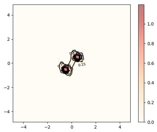
Figure 9.
contour plot with grid points using penalty with .
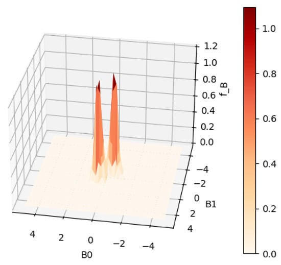
Figure 10.
surface plot with grid points using penalty with .
| sample=sim_sample(n=10000,d=2) |
| grid_beta=grid_set(num_grid_points=40,dim=2) |
| print(grid_beta.numgridpoints()) |
| T=transmatrix(sample,grid_beta) |
| result=rmle(norm_sq,0.4,T) |
| print(result.ev()) |
| [−0.002865326246726808 , −0.010416375635973668] |
| print(result.mode()[:2]) |
| [ [0.39681799850755783, [−0.625, −0.375]], |
| [0.38831830923870914,[0.625, 0.375]]] |
| plot_rmle(result) |
| plot_rmle(result, plt_type= ‘surface’) |
In Figure 11 and Figure 12, estimates with entropy regularization are displayed. Again, these figures can be compared with Figure 3 and Figure 4. The code for entropy regularization is as follows.
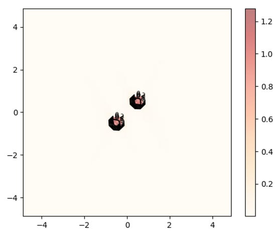
Figure 11.
contour plot with grid points using entropy penalty with .
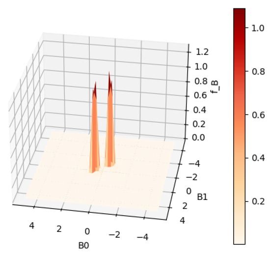
Figure 12.
surface plot with grid points using entropy penalty with .
| result = rmle(entropy, 0.25,T) |
| plot_rmle(result) |
| plot_rmle(result,plt_type=‘surface’) |
Finally, we present an example that demonstrates the usage of the grid_set() function to specify a different range for . The simulated data, in this case, will have modes for that are not covered by the default range . The betas are sampled from the following distribution: . We return to using Sobolev penalty with a large regularization parameter to demonstrate oversmoothing on a smaller grid domain. Results are shown in Figure 13 and Figure 14.
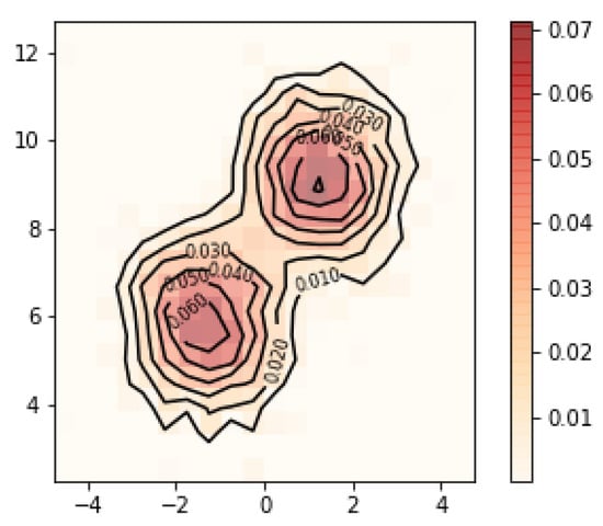
Figure 13.
contour plot with grid points on shifted grid with Sobolev penalty and .
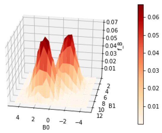
Figure 14.
surface plot with grid points on a shifted grid with Sobolev penalty and .
| cov = [[[1, 0], [0, 1]],[[1, 0], [0, 1]]] |
| mu = [[-1.5,6],[1.5,9]] |
| sample = sim_sample(10000,2,beta_mu = mu,beta_cov = cov) |
| grid_beta_shifted = grid_set(num_grid_points = 20, \ |
| dim = 2, B1_range=[2,13]) |
| T_shifted = transmatrix(sample, grid_beta_shifted) |
| result_shifted = rmle(sobolev_norm_penal,0.5,T_shifted) |
| print(result_shifted.ev()) |
| [0.03520704073478552, 7.524001743037029] |
| print(result_shifted.mode()[0:2]) |
| [[0.07133616078580148, [1.25, 8.875]], |
| [0.0652140364538059, [−1.75, 5.574999999999999]]]] |
| plot_rmle(result_shifted) |
| plot_rmle(result_shifted,plt_type=‘surface’) |
Example 2.
Three-Dimensional Case Two Regressors with Random Intercept
This second example is described by
The example is again presented with simulated data using the same function sim_sample(). The regressors are simulated as follows: are i.i.d and the random coefficients are simulated from .
| from pyrmle import * |
| sample = sim_sample(n = 10000,dim = 3) |
As in the previous example, the program begins by importing the necessary modules and functions. The sim_sample() function generates sample observations based on the aforementioned distributions. This results in a NumPy array.
| grid_beta = grid_set(10,3,B0_range=[−2,4],\ |
| B1_range=[−2,4],B2_range=[−2,4]) |
| print(grid_beta.numgridpoints()) |
| 1000 |
| T = transmatrix(sample,grid_beta) |
The next step is to establish the number of grid points and to generate the transformation using the simulated sample observations. In this case, we first consider 10 grid points in each axis amounting to a total of 1000 grid points. If the user wishes to estimate over a finer grid, it would be more efficient to first determine the smallest possible range of each axis that would fit almost all of the probability mass of . We use a Sobolev penalty with for the first run.
| result = rmle(sobolev_3d,0.6,T) |
| print(result.ev()) |
| [2.458436489282234, 2.25500373629305, 1.9058740990043983] |
| print(result.mode()) |
| [0.08926614291105403, [1.90000000, 1.90000000, 1.90000000]] |
| plot_rmle(result) |
| plot_rmle(result,plt_type=‘surface’) |
In the three-dimensional application, we use the regularization functional sobolev_3d and supply it as an argument to the rmle() function along with the transformation matrix and . No signs of overfitting are observed in Figure 15 and Figure 16, which suggests that a smaller value for can be tried out.
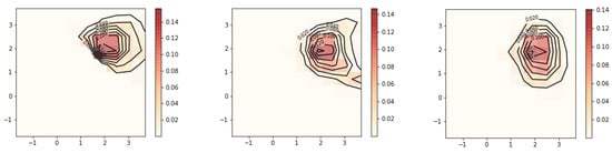
Figure 15.
Contour plots of joint bivariate marginal distributions of : (left), (middle), and (right); Sobolev penalty with .
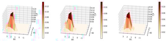
Figure 16.
Surface plots of joint bivariate marginal distributions of : (left), (middle), and (right); Sobolev penalty with .
It is possible to achieve more accurate estimates with more grid points in conjunction with a narrower grid range but with a significantly higher computational cost. We set the number of grid points to 20 on each axis, which amounts to a total of 8000 grid points. The regularization parameter is reduced to . The additional level of discretization due to the increased number of grid points and the smaller domain, together with the smaller , results in an improved estimate as observed in Figure 17 and Figure 18.
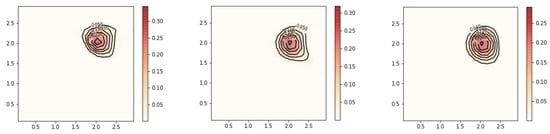
Figure 17.
Contour plots of joint bivariate marginal distributions of : (left), (middle), and (right); Sobolev penalty with .
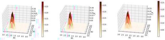
Figure 18.
Surface plots of joint bivariate marginal distributions of : (left), (middle), and (right); Sobolev penalty with .
| grid_beta_alt = grid_set(20,3,B0_range=[0,3],\ |
| B1_range=[0,3],B2_range=[0,3]) |
| print(grid_beta_alt.numgridpoints()) |
| 8000 |
| T2 = transmatrix(sample,grid_beta_alt) |
| result2 = rmle(sobolev_3d,0.3,T2) |
| print(result2.ev()) |
| [2.102855111361121, 2.077365765266784, 1.9697452677152947] |
| print(result2.mode()[0]) |
| [[0.2008050879224736, [2.025, 2.025, 2.025]] |
| plot_rmle(result2) |
| plot_rmle(result2,plt_type=‘surface’) |
The next example will demonstrate the case when the underlying joint density being reconstructed has a single mode at the center of the grid. Both methods of dealing with this issue described in Section 3.1 will be illustrated. Since there were no signs of overfitting in the previous result, we further reduce the regularization to .
| mu = [[0,0,0],[0,0,0],[0,0,0]] |
| sample = sim_sample(n = 5000,dim = 3, \ |
| beta_mu = mu) |
| grid_beta = grid_set(20,3,B0_range=[−1,2], \ |
| B1_range=[−1.5,1.5],B2_range=[−1.5,1.5]) |
| T = transmatrix(sample,grid_beta) |
| result = rmle(sobolev_3d,0.15,T) |
| print(result.ev()) |
| [−0.19254733276928582, 0.005554898823827626, −0.009788891289943112] |
| print(result.mode()) |
| %.14336637945812933 , |
| [−0.024999999999999967, 0.075, −0.075]] |
| plot_rmle(result) |
| plot_rmle(result,plt_type=‘surface’) |
Results are displayed in Figure 19 and Figure 20. The contours show more kinks and appear to be less regular than in Figure 17. This suggests that should not be reduced any further for this data.
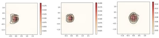
Figure 19.
Contour plots of joint bivariate marginal distributions of : (left), (middle), and (right).
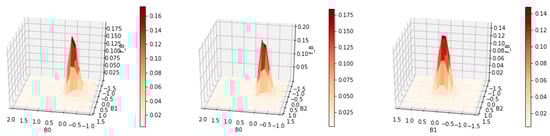
Figure 20.
Surface plots of joint bivariate marginal distributions of : (left), (middle), and (right).
Finally, we show estimates for this test problem with and entropy regularization. Apart from the alternative penalty terms, we replicate the setup of Figure 15 and Figure 16, so results are best compared with these plots. and entropy do not enforce smoothness of the solution as much as the Sobolev penalty, which leads to estimates with less regularity. It is up to the user to decide whether they expect the true solution to be smooth or not and choose the corresponding regularization.
The result with the penalty and is displayed in Figure 21 and Figure 22. The corresponding code is as follows.
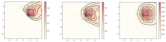
Figure 21.
Contour plots of joint bivariate marginal distributions of : (left), (middle), and (right).
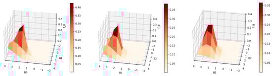
Figure 22.
Surface plots of joint bivariate marginal distributions of : (left), (middle), and (right).
| sample = sim_sample(n = 10000 , d = 3) |
| print(sample) |
| grid_beta = grid_set(10,3,B0_range=[−2,4],\ |
| B1_range =[−2,4],B2_range=[−2,4]) |
| print( grid_beta . numgridpoints ( ) ) |
| 1000 |
| T = transmatrix ( sample , grid_beta ) |
| result = rmle(norm_sq_3d,0.6,T) |
| print(result.ev()) |
| [2.458436489282234, 2.25500373629305, 1.9058740990043983] |
| print(result.mode()) |
| [0.08926614291105403, [1.90000000, 1.90000000, 1.90000000]] |
| plot_rmle (result) |
| plot_rmle (result, plt_type= ‘surface’) |
The result with the entropy penalty and is displayed in Figure 23 and Figure 24. The corresponding code is as follows.
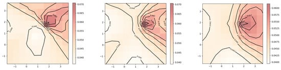
Figure 23.
Contour plots of joint bivariate marginal distributions of : (left), (middle), and (right).
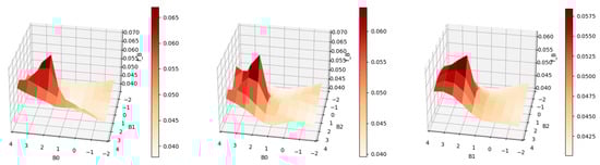
Figure 24.
Surface plots of joint bivariate marginal distributions of : (left), (middle), and (right).
| result = rmle(entropy_3d,0.6,T) |
| plot_rmle(result) |
| plot_rmle(result,plt_type=‘surface’) |
Robustness by Shifting
For the three-dimensional implementation, we found that numerical instabilities of the Python optimization algorithm can occur when the underlying density has a single mode located at the center of the grid. This problem is overcome by simply shifting the density and the data by a constant .
The following example demonstrates how our algorithm can automatically detect if the instability is present by adding c∼ to the intercept. The values a and b are determined by the size of the grid. This applies a transformation that can be back-transformed after estimation by adjusting the grid of . This is repeated for ten different shifts. Then, a simple k-means clustering algorithm using sklearn.cluster.K-means() is applied to the distances of {}. The reconstruction that is closest to the centroid of the largest cluster is then chosen as the solution (also see Figure 25 and Figure 26).
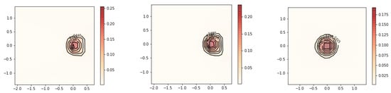
Figure 25.
Contour plots of joint bivariate marginal distributions of : (left), (middle), and (right).
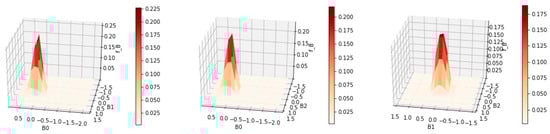
Figure 26.
Surface plots of joint bivariate marginal distributions of : (left), (middle), and (right).
| grid_beta = grid_set(20,3,B0_range=[−1.5,1.5],\ |
| B1_range=[−1.5,1.5],B2_range=[−1.5,1.5]) |
| T = transmatrix(sample,grid_beta) |
| result_shift = rmle(sobolev_3d,0.15,T,shift=True) |
| print(result_shift.ev()) |
| [−0.12974928815245057, −0.004493337754614205, −0.0052980597609372385] |
| print(result_shift.mode()) |
| [[0.14624599807641833, [0.009524681155561987, −0.075, −0.075]] |
| plot_rmle(result) |
| plot_rmle(result_shift,plt_type=‘surface’) |
5. Application to Household Expenditure and Demand
This demonstrates the usefulness of the module in a real data application and shows the user how to load the data into Python from a comma-separated values (CSV) format and how to pre-process it, if necessary, into a usable form. We evaluate household expenditure data from the British Family Expenditure Survey as in [7,16]. The model is the almost-ideal demand system by [25] but with random coefficients instead of fixed coefficients
As discussed in [7], a linear transformation is applied to the regressors before generating the transformation matrix to be used in the algorithm. This is to ensure that the grid is sufficiently covered by the hyperplanes generated by the sample observations. The OLS estimate for the random coefficients suggests that is centered at (0.262755, 0.0048, −0.00069) for a subsample size of . We choose the grid in a way that this potential mode is not in the center.
| data = np.genfromtxt(‘filename.csv’, delimiter=‘,’) |
| data = data[1:−1,1:4] |
| data = data[np.random.randint(1,len(data),5000),:] |
| data = data[∼np.isnan(data).any(axis=1)] |
| ones = np.repeat(1,len(data)) |
| real_data_sample = np.c_[ones, \ |
| 25*data[:,2]−0.3,data[:,1]−5,data[:,0]] |
The code block above loads the data from a csv file, selects a random subsample of 5000 observations, and applies the linear transformations on the data (also see Figure 27 and Figure 28).
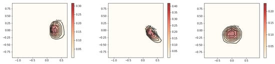
Figure 27.
Contour plots of joint bivariate marginal distributions of : (left), (middle), and (right).
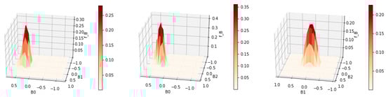
Figure 28.
Surface plots of joint bivariate marginal distributions of : (left), (middle), and (right).
| grid_beta = grid_set(20,3,B0_range=[−0.75,1.25],\ |
| B1_range=[−1,1],B2_range=[−1,1]) |
| T = transmatrix(real_data_sample,grid_beta) |
| result = rmle(sobolev_3d,0.25,T,shift=True) |
| print(result.ev()) |
| [0.2139255519131858, −0.0022826617746834394, −0.10875379495199464] |
| print(result.mode()[0:1]) |
| [[0.19533254824055002, [0.3, −0.05, −0.15000000000000002]] |
| plot_rmle(result) |
| plot_rmle(result,plt_type=‘surface’) |
Included in the module is an option to fit a spline to the estimate . This allows the user to generate smoother plots from the results if they wish. The spline_fit() function takes two essential arguments. The first positional argument is the class RMLEResult object, and the second is the number of grid points on each axis (also see Figure 29 and Figure 30).
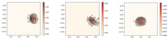
Figure 29.
Contour plots of the spline interpolated joint bivariate marginal distributions of : (left), (middle), and (right).
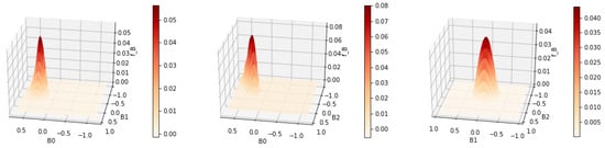
Figure 30.
Surface plots of the spline interpolated joint bivariate marginal distributions of : (left), (middle), and (right).
| spline = spline_fit(result,num_grid_points = 400) |
| plot_rmle(spline) |
| plot_rmle(spline,plt_type=‘surface’) |
Author Contributions
Conceptualization, F.D., E.M. and M.R.; Writing—original draft, F.D., E.M. and M.R.; Writing—review and editing, F.D., E.M. and M.R. All authors have read and agreed to the published version of the manuscript.
Funding
This research received no external funding.
Data Availability Statement
The original contributions presented in this study are included in the article. Further inquiries can be directed to the corresponding author.
Conflicts of Interest
The authors declare no conflicts of interest.
References
- Beran, R.; Hall, P. Estimating coefficient distributions in random coefficient regressions. Ann. Stat. 1992, 20, 1970–1984. [Google Scholar] [CrossRef]
- Beran, R.; Feuerverger, A.; Hall, P. On nonparametric estimation of intercept and slope distributions in random coefficient regression. Ann. Stat. 1996, 24, 2569–2592. [Google Scholar] [CrossRef]
- Hoderlein, S.; Klemelä, J.; Mammen, E. Analyzing the random coefficient model nonparametrically. Econom. Theory 2010, 26, 804–837. [Google Scholar] [CrossRef]
- Fox, J.T.; Kim, K.I.; Ryan, S.P.; Bajari, P. A simple estimator for the distribution of random coefficients. Quant. Econ. 2011, 2, 381–418. [Google Scholar] [CrossRef]
- Heiss, F.; Hetzenecker, S.; Osterhaus, M. Nonparametric estimation of the random coefficients model: An elastic net approach. J. Econom. 2022, 229, 299–321. [Google Scholar] [CrossRef]
- Breunig, C.; Hoderlein, S. Specification testing in random coefficient models. Quant. Econ. 2018, 9, 1371–1417. [Google Scholar] [CrossRef]
- Dunker, F.; Eckle, K.; Proksch, K.; Schmidt-Hieber, J. Tests for qualitative features in the random coefficients model. Electron. J. Stat. 2019, 13, 2257–2306. [Google Scholar] [CrossRef]
- Gaillac, C.; Gautier, E. Adaptive estimation in the linear random coefficients model when regressors have limited variation. Bernoulli 2022, 28, 504–524. [Google Scholar] [CrossRef]
- Hermann, P.; Holzmann, H. Bounded support in linear random coefficient models: Identification and variable selection. Econom. Theory 2024, 41, 947–976. [Google Scholar] [CrossRef]
- Holzmann, H.; Meister, A. Rate-optimal nonparametric estimation for random coefficient regression models. Bernoulli 2020, 26, 2790–2814. [Google Scholar] [CrossRef]
- Lim, K.; Ye, T.; Han, F. A sliced Wasserstein and diffusion approach to random coefficient models. arXiv 2025, arXiv:2502.04654. [Google Scholar]
- Werner, F.; Hohage, T. Convergence rates in expectation for Tikhonov-type regularization of inverse problems with Poisson data. Inverse Probl. 2012, 28, 104004. [Google Scholar] [CrossRef]
- Hohage, T.; Werner, F. Iteratively regularized Newton-type methods for general data misfit functionals and applications to Poisson data. Numer. Math. 2013, 123, 745–779. [Google Scholar] [CrossRef]
- Hohage, T.; Werner, F. Inverse problems with Poisson data: Statistical regularization theory, applications and algorithms. Inverse Probl. 2016, 32, 093001. [Google Scholar] [CrossRef]
- Dunker, F.; Hohage, T. On parameter identification in stochastic differential equations by penalized maximum likelihood. Inverse Probl. 2014, 30, 095001. [Google Scholar] [CrossRef][Green Version]
- Dunker, F.; Mendoza, E.; Reale, M. Regularized maximum likelihood estimation for the random coefficients model. Econom. Rev. 2025, 44, 192–213. [Google Scholar] [CrossRef]
- Harris, C.R.; Millman, K.J.; van der Walt, S.J.; Gommers, R.; Virtanen, P.; Cournapeau, D.; Wieser, E.; Taylor, J.; Berg, S.; Smith, N.J.; et al. Array programming with NumPyf. Nature 2020, 585, 357–362. [Google Scholar] [CrossRef]
- Jones, E.; Oliphant, T.; Peterson, P. SciPy: Open Source Scientific Tools for Python. 2001. Available online: https://www.scipy.org (accessed on 28 October 2025).
- Byrd, R.H.; Hribar, M.E.; Nocedal, J. An interior point algorithm for large-scale nonlinear programming. SIAM J. Optim. 1999, 9, 877–900. [Google Scholar] [CrossRef]
- Lepskiĭ, O.V. A problem of adaptive estimation in Gaussian white noise. Theory Probab. Its Appl. 1990, 35, 459–470. [Google Scholar] [CrossRef]
- Lepskiĭ, O.V. Asymptotically minimax adaptive estimation. I. Upper bounds. Optimally adaptive estimates. Theory Probab. Its Appl. 1991, 36, 645–659. [Google Scholar] [CrossRef]
- Lepskiĭ, O.V. Asymptotically minimax adaptive estimation. II. Schemes without optimal adaptation. Adaptive estimates. Theory Probab. Its Appl. 1992, 37, 468–481. [Google Scholar] [CrossRef]
- Lepskiĭ, O.V. On problems of adaptive estimation in white Gaussian noise. Top. Nonparametric Estim. 1992, 12, 87–106. [Google Scholar]
- Mathé, P. The Lepskii principle revisited. Inverse Probl. 2006, 22, L11. [Google Scholar] [CrossRef]
- Deaton, A.; Muellbauer, J. An almost ideal demand system. Am. Econ. Rev. 1980, 70, 312–326. [Google Scholar]


Disclaimer/Publisher’s Note: The statements, opinions and data contained in all publications are solely those of the individual author(s) and contributor(s) and not of MDPI and/or the editor(s). MDPI and/or the editor(s) disclaim responsibility for any injury to people or property resulting from any ideas, methods, instructions or products referred to in the content. |
© 2025 by the authors. Licensee MDPI, Basel, Switzerland. This article is an open access article distributed under the terms and conditions of the Creative Commons Attribution (CC BY) license (https://creativecommons.org/licenses/by/4.0/).