Fuzzy Model Predictive Tracking Control for Boiler-Turbine Systems with Disturbances and Input Constraints

Abstract

During the actual operation of a boiler-turbine system (BTS), it inevitably encounters various unknown disturbances and model uncertainty. Additionally, due to physical limitations, there are constraints on both the magnitude and the change rate of unit controls. These factors generally cause instability of the BTS and prevent it from achieving zero-offset tracking of load commands. To address this issue, this paper proposes a fuzzy model predictive tracking control (FMPTC) scheme for the nonlinear BTS with disturbances and input constraints. With the proposed FMPTC scheme, the closed-loop system is theoretically proved to be asymptotically stable and offset-free in output tracking; meanwhile, the constraints on the input magnitude and change rate are satisfied by both the free control variable and the future control input in the form of the state feedback law. The simulation results for a 300 MW unit demonstrate the advantages of the proposed control scheme.

1. Introduction

Despite the growing attention to the new energy industry in recent years, coal-fired power plants remain pivotal to global power generation [1,2]. For a boiler-turbine system (BTS), a core operational requirement is to rapidly track load demands from automatic dispatch systems or operator inputs while maintaining throttle steam pressure within a specified safe range. Conventional proportional–integral–derivative (PID) controllers are widely adopted for BTS control due to their simplicity [3,4,5]. However, the BTS exhibits inherent characteristics such as tight input constraints, significant nonlinearity across a wide operating range, and susceptibility to external disturbances and model uncertainties, which means that PID controllers often fail to meet high-performance control demands [6,7].

Model predictive control (MPC) has emerged as a promising solution for process control, as it explicitly handles constraints during controller synthesis [8,9,10,11]. For BTS applications, prior studies have developed dynamic matrix controllers based on step-response models [9,10] and generalized predictive controllers using controlled auto-regressive integrated moving average models [11]. Simulation results indicate that linear MPCs outperform PID controllers in most cases. Nevertheless, due to the nonlinearity of the BTS, linear MPCs often fail to meet design specifications when operating across a wide range of load conditions. To address this nonlinearity challenge, nonlinear MPC (NMPC) schemes have been proposed for BTS control, which involve solving nonlinear numerical optimization problems at each sampling instant [12]. A major drawback of such approaches is the high computational cost of nonlinear optimization. To mitigate this issue, a nonlinear multivariable NMPC scheme integrating neuro-fuzzy network modelling was developed, transforming the nonlinear optimization problem into a convex one solvable via Karush–Kuhn–Tucker conditions [13]. Another study designed an NMPC controller for power output regulation based on the mixed logical dynamical model of the BTS, avoiding excessive complexity and implementation costs [14]. Additionally, an MPC algorithm using successive online linearization of the nonlinear BTS model was proposed to enhance computational efficiency [15]. While these nonlinear MPC methods improve computational speed, they lack theoretical guarantees for the stability of the closed-loop system.

To balance closed-loop stability and computational efficiency, stable fuzzy model predictive control schemes based on the Takagi–Sugeno (T-S) fuzzy model have been investigated [16,17,18]. The T-S fuzzy model approximates nonlinear systems by blending multiple local linear models via membership functions, and it can achieve arbitrary approximation accuracy for smooth functions with a sufficient number of rules [19,20,21]. However, existing fuzzy MPC formulations have notable gaps. The schemes in [16,19] only consider input magnitude constraints while neglecting input change rate constraints. The approach in [18] imposes constraints solely on free control variables, ignoring constraints on future control inputs. In the disturbance-observer-based fuzzy model predictive control scheme [22,23], the baseline fuzzy MPC controller is designed to ensure that both the free control variable and the future state feedback-based control inputs strictly comply with the predefined constraints on input magnitude and rate of change. However, the overall control schemes do not theoretically guarantee that the input constraints are satisfied. Thus, no existing fuzzy MPC strategy fully addresses all input constraints for BTS control.

Another key concern in practical BTS control is the output tracking performance of the closed-loop system [24]. MPC performance heavily relies on model accuracy: an ideal predictive model enables exact set-point tracking, while model mismatches often lead to steady-state offsets in controlled outputs. Two primary approaches have been proposed to mitigate model mismatches and eliminate offsets [25,26]. The first augments the MPC controller with integral action, incorporating tracking error integration into the objective function [25,26,27]. The second integrates disturbance terms into the process model to account for unmodeled dynamics [25,26]. Offset-free MPC schemes based on disturbance modelling have been widely explored [28,29,30,31,32,33,34,35]. Notably, a general disturbance model (GDM) including both state and output disturbance terms was developed to accurately characterize actual process disturbances [27]. By estimating these disturbance terms, a steady-state target calculator (SSTC) adjusts steady-state targets to eliminate disturbance-induced offsets, enabling offset-free tracking. However, existing offset-free MPC schemes based on disturbance models lack theoretical stability guarantees for the closed-loop system [27,28,31,32]. Furthermore, most of these schemes are designed for linear systems [27,28,29,30,31,32,33], making them unsuitable for nonlinear BTS operating across a wide load range, where zero-offset tracking cannot be guaranteed.

Given the aforementioned limitations, this study proposes a fuzzy model predictive tracking control (FMPTC) scheme for a 300 MW subcritical BTS subject to disturbances and input constraints. To accurately characterize the practical BTS, a general disturbance model (GDM) is developed by integrating disturbance terms into the T-S fuzzy model, which lumps the total effects of unknown external disturbances and model uncertainty. Utilizing disturbance estimates obtained from a fuzzy extended state observer, a steady-state target calculator dynamically adjusts the steady-state targets to counteract the disturbance effect. The control law of the proposed FMPTC scheme is derived by solving a semidefinite programming problem constrained by a set of linear matrix inequalities (LMIs). The main contributions of this work are as follows:

(1)

Compared with existing studies, the proposed FMPTC scheme guarantees that the closed-loop system is asymptotically stable and the output offset-free tracking performance for the nonlinear system is achieved, while the constraints on the input magnitude and change rate are satisfied by both the free control variable and the future control input in the form of the state feedback law.

(2)

Simulation results demonstrate that the closed-loop system maintains offset-free set-point tracking under full operating conditions, even in the presence of input constraints, external disturbances from any channel, and model uncertainties.

The remainder of this paper is organized as follows: Section 2 presents the BTS dynamics of a subcritical unit and preliminaries involving the T-S fuzzy modelling. Section 3 details the design of the FMPTC scheme, and Section 4 validates the proposed scheme through simulation results. Section 5 draws the main conclusions.

Notation: x_k+i|k denotes the predicted state at sampling instant k + i based on the current state x_k|k. I represents the identity matrix with dimensions matching the context. For any symmetrical matrix A, the notation A > 0 indicates that A is a positive definite matrix. For any two symmetrical matrices A and B, A > B signifies that the matrix A-B is positive definite. A star (*) in a matrix denotes the transposed element located at the symmetric position. At the sampling instant k, for normalized membership functions w_i, the antecedent variable z and matrices X_i.

$$w_i:=w_i\left(z_k\right), w_{i+}:=w_i\left(z_{k+1}\right); X_z:={\displaystyle \sum _i{w}_i{X}_i}, X_{z+}:={\displaystyle \sum _i{w}_{i+}{X}_i}, X_z^{-1}:={\left({\displaystyle \sum _i{w}_i{X}_i}\right)}^{-1};$$

$$X_{zz}:={\displaystyle \sum _{i=1}{\displaystyle \sum _j{w}_i{w}_j{X}_{ij}}}, X_{zz+}:={\displaystyle \sum _{i=1}{\displaystyle \sum _j{w}_{i+}{w}_{j+}{X}_{ij}}}, X_{zz}^{-1}:={\left({\displaystyle \sum _{i=1}{\displaystyle \sum _j{w}_i{w}_j{X}_{ij}}}\right)}^{-1}.$$

2. System Description and Preliminaries

2.1. Boiler-Turbine System Dynamics

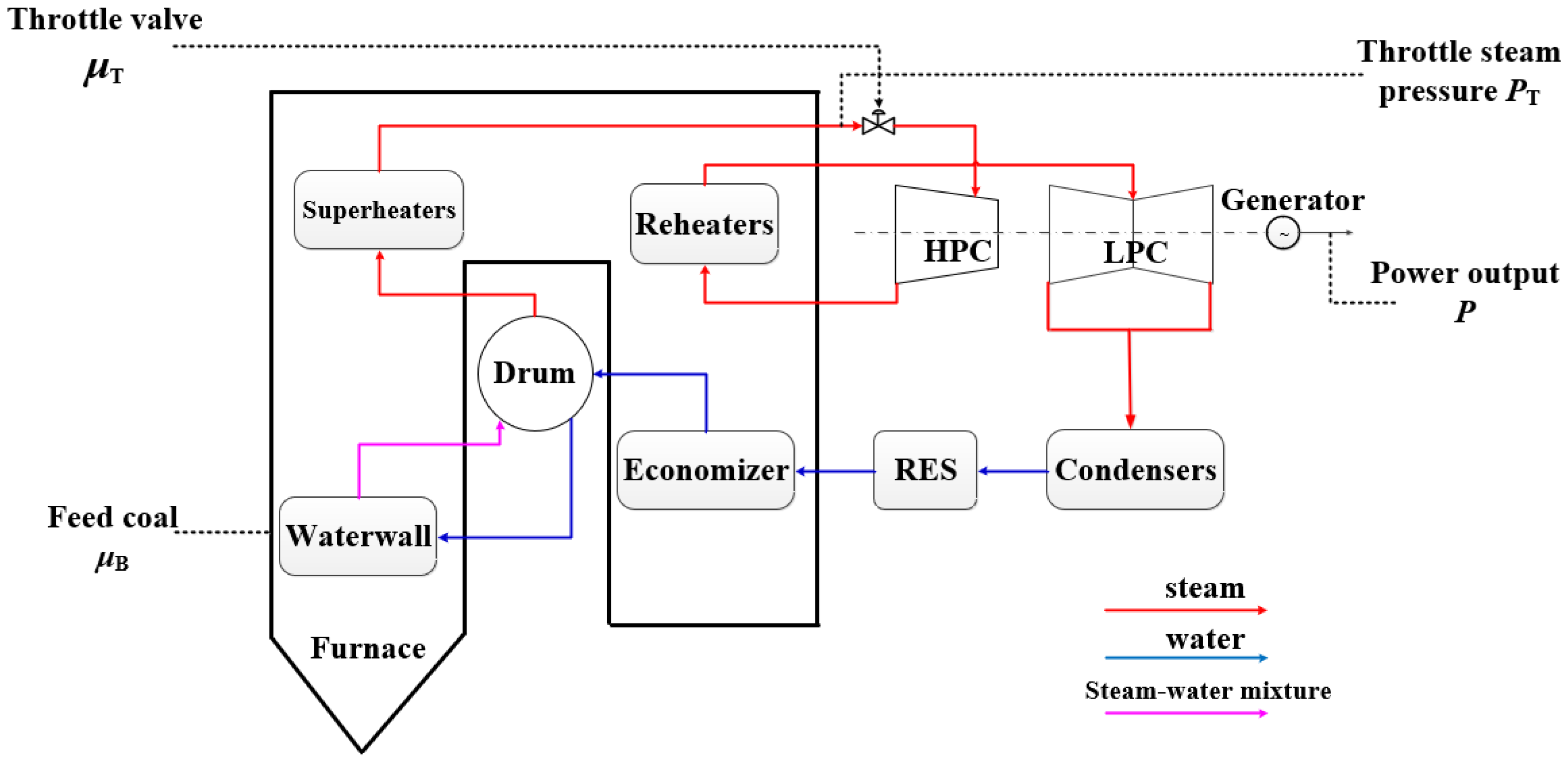
This study focuses on a 300 MW subcritical unit, whose simplified schematic diagram is shown in Figure 1. The boiler converts the chemical energy stored in pulverized coal into thermal energy of steam through thermal radiation and convection, a process that occurs sequentially in a series of heat exchangers—including the waterwall, superheaters, reheaters, and economizer. This thermal energy is subsequently converted into rotational mechanical energy in the turbine’s high-pressure cylinder and low-pressure cylinder, in turn. Owing to the coaxial design of the turbine and generator, the mechanical energy is ultimately transformed into electrical power. See [36] for details regarding the unit’s mechanism.

The dynamics of the boiler-turbine system is characterized by a fourth-order nonlinear model, which is given as follows [22,37]:

$$\left\{\begin{array}{l}{\dot{x}}_1=-0.01x_1+2.623x_2{u}_1\\ {\dot{x}}_2=0.0428(0.0138x_3{}^2+0.15x_3+4.17)\sqrt{x_3-x_2}-0.0451x_2{u}_1\\ {\dot{x}}_3={\displaystyle \frac{\mathrm{20,237.25}{x}_4-1669.8x_1-318.28}{175.39(1.06x_3-5.16)(-1.434x_3{}^2+13.578x_3+1547)}}-{\displaystyle \frac{73.8(0.0138x_3{}^2+0.15x_3+4.17)\sqrt{x_3-x_2}}{175.39(1.06x_3-5.16)}}\\ {\dot{x}}_4=-0.005x_4+0.005u_2\\ y_1=x_1\\ y_2=x_2\end{array}\right.$$

(1)

where the state variables x₁, x₂, x₃, and x₄ denote the electric power P (MW), the throttle steam pressure P_T (MPa), the drum steam pressure P_D (MPa), and the flow rate of pulverized coal entering the furnace D_cf (kg/s), respectively; the control inputs u₁ and u₂ correspond to the turbine throttle valve opening u_T and the flow rate of the feed coal u_B (kg/s), respectively; the outputs y₁ and y₂ are the electric power P (MW) and throttle pressure P_T (MPa), respectively.

Owing to the physical limitations of the actuators, constraints exist on both the magnitude and rate of change in the control inputs. In accordance with the actuator specifications and operational requirements, the input constraints are defined as follows:

$$\left\{\begin{array}{l}0\le u_1\le 1\\ 0\le u_2\le 45\\ -0.015\le {\dot{u}}_1\le 0.015\\ -2\le {\dot{u}}_2\le 2\end{array}\right.$$

(2)

See [37] for details regarding the mechanism modelling of the boiler-turbine system.

2.2. T-S Fuzzy Modelling

The boiler-turbine nonlinear dynamics (1) is rewritten as

$$\left\{\begin{array}{l}\dot{x}=F\left(x,u\right)\\ y=Cx\end{array}\right.$$

(3)

where $x\in {\Re }^n$, $u\in {\Re }^m$ and $y\in {\Re }^p$ are the state, input, and output vectors, respectively; the nonlinear vector function F: ${\Re }^n\times {\Re }^m\to {\Re }^n$ and C = [0100, 1000].

The T-S fuzzy model is usually described as a series of IF-Then rules, of which the i-th one is

r_i: if z_k is Γ_i, then

$$\left\{\begin{array}{l}{x}_{k+1}=A_i{x}_k+B_i{u}_k+R_i\\ y_k=C{x}_k\end{array}\right., i=1,2,\dots ,N$$

(4)

where r_i denotes the i-th rule, N the number of rules, z_k the antecedent variable, Γ_i the i-th fuzzy set, A_i, B_i, and R_i the system matrices of the i-th local model, and k the k-th sampling instant.

In order to develop a satisfactory fuzzy model, a systematic gap-based T-S fuzzy modelling approach is adopted [22,23]. The global T-S fuzzy model is developed as follows:

$$\left\{\begin{array}{l}{x}_{k+1}=A_z{x}_k+B_z{u}_k+R_z\\ y_k=C{x}_k\end{array}\right.$$

(5)

where $A_z={\displaystyle \sum _{i=1}^N{w}_i{A}_i}$, $B_z={\displaystyle \sum _{i=1}^N{w}_i{B}_i}$, and $R_z={\displaystyle \sum _{i=1}^N{w}_i{R}_i}$ with the membership functions $w_i$, $w_i\ge 0$, ${\displaystyle \sum _{i=1}^N{w}_i=1}$. In addition, the input constraints in the discrete-time domain are denoted as

$$\left\{\begin{array}{l}{u}_{\min }\le u_k\le u_{\max }\\ \Delta u_{\min }\le \Delta u_k\le \Delta u_{\max }\end{array}\right.$$

(6)

where u_min and u_max are the lower and upper bounds of the input, respectively; ∆u_min and ∆u_max are the lower and upper bounds of the incremental control input, respectively.

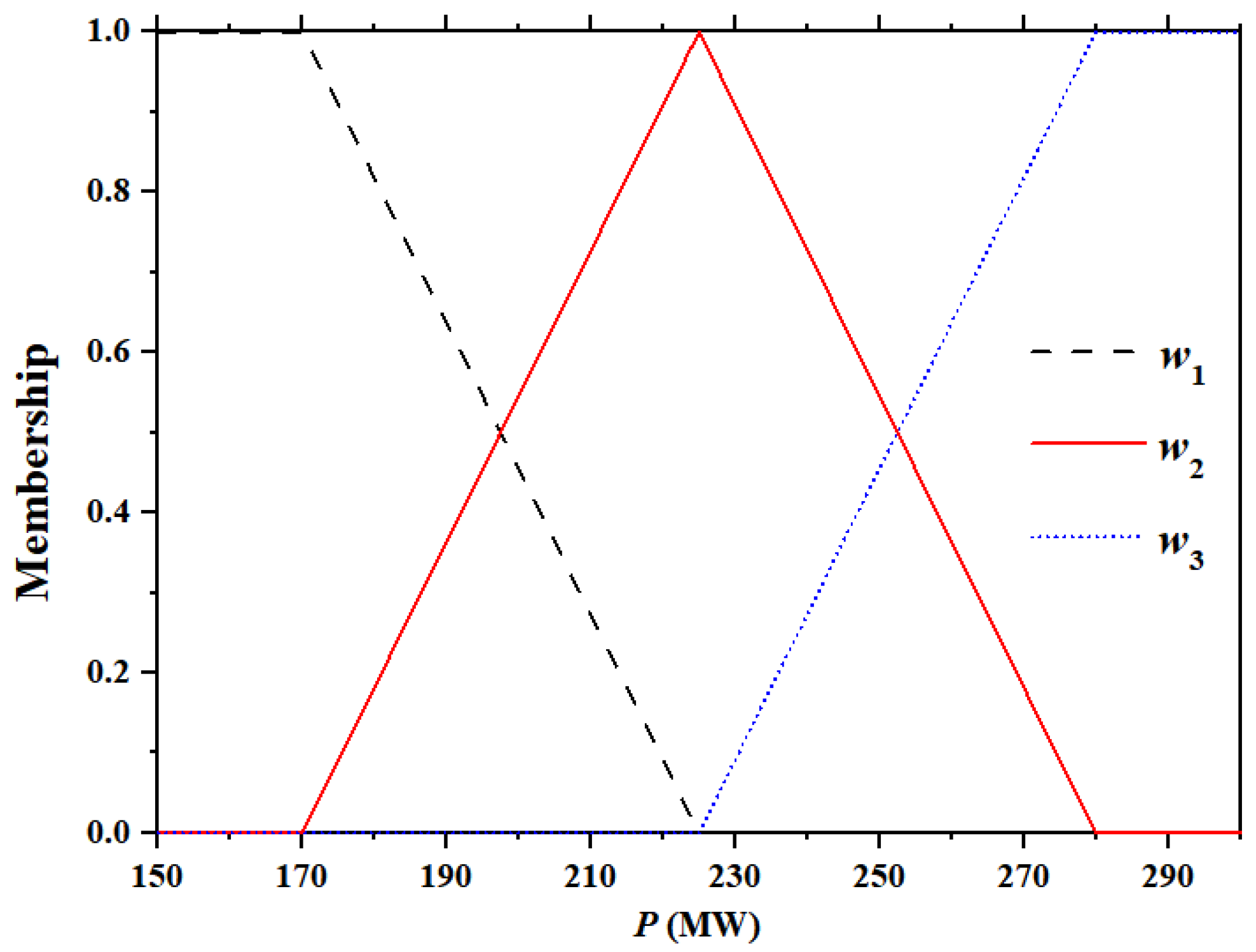
In this study, the power output P is selected as the antecedent variable to characterize the operational state of the BTS, as all other state variables of the BTS are dependent on it. The operation range under investigation is defined as [150 MW, 300 MW]. Three linearization operation points—specifically, 170 MW, 225 MW, and 280 MW—are determined via the systematic gap-based T-S fuzzy modelling approach. Subsequently, the T-S fuzzy model is constructed by blending the local linearized models corresponding to these operating points, with the membership functions illustrated in Figure 2.

3. Fuzzy Model Predictive Tracking Control Scheme for the Boiler-Turbine System

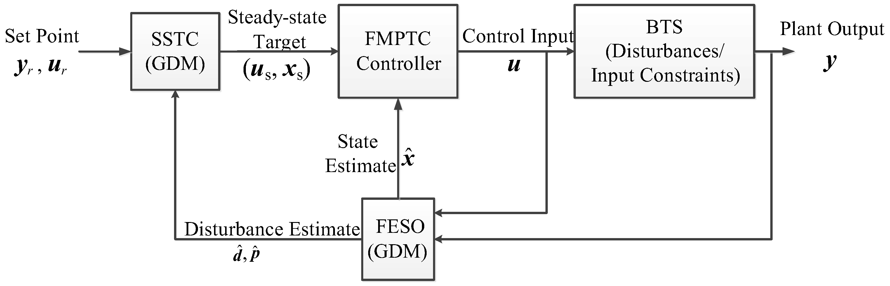
The proposed FMPTC scheme for the BTS is shown in Figure 3. The GDM was first developed to represent the actual BTS by integrating disturbance terms into the fuzzy model. The fuzzy extended state observer (FESO) estimates the disturbance terms, and the estimates are applied to the SSTC to determine the steady-state input and state targets. With the steady-state targets and the state estimates, the control inputs are then determined by the FMPTC algorithm.

3.1. General Disturbance Model

Since the approximation error of the fuzzy model, the external disturbance and model uncertainties inevitably exist in practical applications, the GDM is developed by incorporating two additional disturbance terms $d\in {\Re }^{sd}$ and $p\in {\Re }^{sp}$ into the fuzzy model (5), which, respectively, lump the comprehensive effects of the aforementioned factors on the system states and outputs. Thus, the GDM enables accurate characterization of the actual operating behaviour of the BTS

$$\left\{\begin{array}{l}{x}_{k+1}=A_z{x}_k+B_z{u}_k+R_z+G_{dz}{d}_k\\ y_k=C{x}_k+G_{pz}{p}_k\end{array}\right.$$

(7)

where $G_{dz}={\displaystyle \sum _{i=1}^N{w}_i{G}_{d,i}}$, $G_{pz}={\displaystyle \sum _{i=1}^N{w}_i{G}_{p,i}}$ with G_d,i and G_p,i being the disturbance gain matrices of the i-th local disturbance model on the state and output disturbance terms d and p, respectively.

Remark 1.

It can be seen that the input disturbance is a special case of the state disturbance where G_d,i is set equal to B_i. The determination principle of G_d,i and G_p,i refers to the paper [28]. In addition, the disturbance model (7) is the generalization of the ones in [18,19] where the state and output disturbance terms share a signal.

3.2. Fuzzy Extended State Observer

Since the state variable x₄ and the disturbance terms are unmeasurable, an FESO is designed. First, to ensure the observability of the GDM, the following condition should be satisfied [28,38]

$$rank\left[\begin{array}{lll}I-A_i& -G_{d,i}& 0\\ C& 0& G_{p,i}\end{array}\right]=n+sd+sp, i=1,2,\dots ,N$$

(8)

With the antecedent variable measurable, the FESO is constructed as follows:

$$\left\{\begin{array}{l}\left[\begin{array}{c}{\widehat{x}}_{k+1}\\ {\widehat{d}}_{k+1}\\ {\widehat{p}}_{k+1}\end{array}\right]=\left[\begin{array}{ccc}{A}_z& G_{dz}& 0\\ 0& I& 0\\ 0& 0& I\end{array}\right]\left[\begin{array}{l}{\widehat{x}}_k\\ {\widehat{d}}_k\\ {\widehat{p}}_k\end{array}\right]+\left[\begin{array}{c}{B}_z\\ 0\\ 0\end{array}\right]u_k+\left[\begin{array}{c}{R}_z\\ 0\\ 0\end{array}\right]+\left[\begin{array}{c}{L}_z^x\\ L_z^d\\ L_z^p\end{array}\right]\left(y_k-{\widehat{y}}_k\right)\\ {\widehat{y}}_k=\left[C 0 G_{pz}\right]\left[\begin{array}{l}{\widehat{x}}_k\\ {\widehat{d}}_k\\ {\widehat{p}}_k\end{array}\right]\end{array}\right.$$

(9)

where the symbol “^” represents the estimation, and $L={\left[L_z^x{}^T,L_z^d{}^T,{L_z^p}^T\right]}^T$ is the fuzzy observer gain with the state observer gain $L_z^x\in {\Re }^{n\times p}$, the state disturbance observer gain $L_z^d\in {\Re }^{sd\times p}$ and the output disturbance observer gain $L_z^x\in {\Re }^{sp\times p}$, respectively. Specifically, $L={\displaystyle \sum _{l=1}^N{w}_i{L}_l}$ in which $L_l={\left[L_l^x{}^T,L_l^{dT},L_l^{pT}\right]}^T$ is the l-th local observer gain to be determined.

Subtracting (9) from (7), one has

$$\left[\begin{array}{c}{\tilde{x}}_{k+1}\\ {\tilde{d}}_{k+1}\\ {\tilde{p}}_{k+1}\end{array}\right]=\left(\left[\begin{array}{ccc}{A}_z& G_{dz}& 0\\ 0& I& 0\\ 0& 0& I\end{array}\right]+\left[\begin{array}{c}{L}_z^x\\ L_z^d\\ L_z^p\end{array}\right]\left[C 0 G_{pz}\right]\right)\left[\begin{array}{l}{\tilde{x}}_k\\ {\tilde{d}}_k\\ {\tilde{p}}_k\end{array}\right]$$

(10)

where the symbol “~” denotes the estimation error.

Theorem 1

([20,39]). The estimation error system (10) is globally exponentially stable if there exists a positive definite symmetric matrix P, and a set of matrices Q_l, l = 1, 2, …, N, such that the following LMIs are satisfied

$$\left[\begin{array}{cc}P& P{\tilde{A}}_l+Q_l{\tilde{C}}_j\\ \left(*\right)& P\end{array}\right]>0, j=1,2,\dots ,N, l=1,2,\dots ,N$$

(11)

where ${\tilde{A}}_l=\left[\begin{array}{ccc}{A}_l& G_{d,l}& 0\\ 0& I& 0\\ 0& 0& I\end{array}\right]$ and ${\tilde{C}}_j=\left[C 0 G_{p,j}\right]$. Then L_l is determined

$$L_l=P^{-1}{Q}_l, l=1,2,\dots ,N$$

(12)

3.3. Steady-State Target Calculator

Next, the estimates of disturbance terms are applied to develop the SSTC, which shifts the steady-state targets to remove the disturbance effect from the controlled variables [27,28]

$$\underset{x_s,u_s}{\min }{\left(u_r-u_s\right)}^T{R}_s\left(u_r-u_s\right)$$

(13)

s.t

$$\left[\begin{array}{cc}I-A_z& -B_z\\ C& 0\end{array}\right]\left[\begin{array}{l}{x}_s\\ u_s\end{array}\right]=\left[\begin{array}{l}{G}_{dz}{\widehat{d}}_k+R_z\\ -G_{pz}{\widehat{p}}_k+y_r\end{array}\right]$$

(14)

$$u_{\min }\le u_s\le u_{\max }$$

(15)

where R_s is a weighting matrix; x_s and u_s are the steady-state and input targets to be determined; y_r and u_r are the set points of the outputs and inputs, respectively; ${\widehat{d}}_k$ and ${\widehat{p}}_k$ are the estimates of the state and output disturbance terms, respectively.

Subtracting (14) from (7) results in

$$\left\{\begin{array}{l}{\stackrel{⌢}{x}}_{k+1}=A_z{\stackrel{⌢}{x}}_k+B_z{\stackrel{⌢}{u}}_k+G_{dz}{\tilde{d}}_k\\ {\stackrel{⌢}{y}}_k=C{\stackrel{⌢}{x}}_k+G_{pz}{\tilde{p}}_k\end{array}\right.$$

(16)

where ${\stackrel{⌢}{x}}_k=x_k-x_s$,${\stackrel{⌢}{u}}_k=u_k-u_s$, and ${\stackrel{⌢}{y}}_k=y_k-y_r$ are the shifted states, inputs, and outputs, respectively.

3.4. Fuzzy Model Predictive Tracking Controller

With the exponentially stable FESO (9), the estimation errors ${\widehat{d}}_k$ and ${\widehat{p}}_k$ are bounded and gradually decrease to zero. Thus, the nominal model of (16), as follows, is utilized as the predictive model for the FMPTC controller design [19]

$$\left\{\begin{array}{l}{\stackrel{⌢}{x}}_{k+i+1|k}=A_z{\stackrel{⌢}{x}}_{k+i|k}+B_z{\stackrel{⌢}{u}}_{k+i|k}\\ {\stackrel{⌢}{y}}_{k+i|k}=C{\stackrel{⌢}{x}}_{k+i|k}\end{array}\right., i\ge 0$$

(17)

In addition, the following infinite-horizon objective function is adopted for the optimization formulation [40]

$$J_{0,k}^{\infty }={\displaystyle \sum _{i=0}^{\infty }\left[{\stackrel{⌢}{x}}_{k+i|k}^{T}Q{\stackrel{⌢}{x}}_{k+i|k}+{\stackrel{⌢}{u}}_{k+i|k}^{T}R{\stackrel{⌢}{u}}_{k+i|k}\right]}$$

(18)

where Q and R are positive definite symmetric weighting matrices for the shifted states and inputs, respectively.

The control inputs are determined by the following Theorem 2. The detailed proof is given in Appendix A.

Theorem 2.

Consider the discrete-time fuzzy system (7) under the input constraints (6) in which $\Delta u_{\min }<0$ and $\Delta u_{\max }>0$. Suppose the following conditions.

C1. The LMIs (11) admit a positive definite matrix P, and matrices Q_l, l =1, 2, …, N;

C2. There exist solutions (x_s,u_s) to the quadratic programming problem (13)–(15);

C3. The total dimensions of disturbance terms are equal to the number of outputs, namely, sd + sp = p;

C4. There exists a control move ${\stackrel{⌢}{u}}_{k|k}$, matrices Y_i, G_i, slack matrices $Q_{ij}^l={\left(Q_{ji}^l\right)}^T$, symmetric matrices ${\tilde{S}}_i>0$,  $Q_{ii}^l$, i, j, l = 1, 2,…, N, and an upper bound of the infinite horizon objective function γ, such that the following semidefinite programming problem is feasible:

$$\underset{{\stackrel{⌢}{u}}_{k|k},Y_i,G_i,Q_{ij}^k,{\tilde{S}}_i,\gamma }{{\displaystyle \min }}\gamma$$

(19)

s.t

Equations (20)–(27) are satisfied, then a free control input $u_{k|k}={\stackrel{⌢}{u}}_{k|k}+u_s$ and a nonparallel distributed compensation (non-PDC) $u_{k+i|k}=-Y_z{G}_z^{-1}{\stackrel{⌢}{x}}_{k+i|k}+u_s$, i ≥ 1 can be determined such that both of them satisfy the input constraints, and the closed-loop system is asymptotically stable and offset-free in output tracking.

$$n_l=\left[\begin{array}{ccccc}1& \left(*\right)& \left(*\right)& \left(*\right)& \left(*\right)\\ A_z{\widehat{x}}_{s,k}+B_z{\stackrel{⌢}{u}}_{k|k}\hfill & \hfill {\tilde{S}}_l/2\hfill & \hfill 0\hfill & \hfill 0\hfill & \hfill 0\hfill \\ Q^{\raisebox{1ex}{$1$}\!\left/ \!\raisebox{-1ex}{$2$}\right.}{\widehat{x}}_{s,k}\hfill & \hfill 0\hfill & \hfill \gamma I/2\hfill & \hfill 0\hfill & \hfill 0\hfill \\ A_z{e}_b\hfill & \hfill 0\hfill & \hfill 0\hfill & \hfill {\tilde{S}}_l/2\hfill & \hfill 0\hfill \\ R^{\raisebox{1ex}{$1$}\!\left/ \!\raisebox{-1ex}{$2$}\right.}{\stackrel{⌢}{u}}_{k|k}\hfill & \hfill 0\hfill & \hfill 0\hfill & \hfill 0\hfill & \hfill \gamma I\hfill \end{array}\right]>0, l=1,2,\dots ,N$$

(20)

$$r_{ii}^l\ge Q_{ii}^l, i,l=1,2,\dots ,N$$

(21)

$$r_{ij}^l+r_{ji}^l\ge Q_{ij}^l+Q_{ji}^l, j>i, i,j,l=1,2,\dots ,N$$

(22)

$${\Psi }_l=\left[\begin{array}{cccc}{Q}_{11}^l& Q_{12}^l& \dots & Q_{1N}^l\\ Q_{21}^l& Q_{22}^l& \dots & Q_{2N}^l\\ ⋮& ⋮& \ddots & ⋮\\ Q_{N1}^l& \dots & Q_{N(N-1)}^l& Q_{NN}^l\end{array}\right]>0, l=1,2,\dots ,N$$

(23)

$$u_{\min }-u_s\le {\stackrel{⌢}{u}}_{k|k}\le u_{\max }-u_s$$

(24)

$$\Delta u_{\min }+u_{k-1}-u_s\le {\stackrel{⌢}{u}}_{k|k}\le \Delta u_{\max }+u_{k-1}-u_s$$

(25)

$$q_{1,i}>0, i=1,2,\dots ,N$$

(26)

$$q_{2,i}>0, i=1,2,\dots ,N$$

(27)

where

$$r_{ij}^l=\left[\begin{array}{cccc}{G}_i+G_j^T-{\tilde{S}}_i\hfill & \hfill \left(*\right)\hfill & \hfill \left(*\right)\hfill & \hfill \left(*\right)\hfill \\ A_i{G}_j-B_i{Y}_j\hfill & \hfill {\tilde{S}}_l\hfill & \hfill 0\hfill & \hfill 0\hfill \\ Q^{\raisebox{1ex}{$1$}\!\left/ \!\raisebox{-1ex}{$2$}\right.}{G}_i\hfill & \hfill 0\hfill & \hfill \gamma I\hfill & \hfill 0\hfill \\ R^{\raisebox{1ex}{$1$}\!\left/ \!\raisebox{-1ex}{$2$}\right.}{Y}_i\hfill & \hfill 0\hfill & \hfill 0\hfill & \hfill \gamma I\hfill \end{array}\right], i,j,l=1,2,\dots ,N$$

(28)

$$q_{1,i}=\left[\begin{array}{cc}\hfill G_i+G_i^T-{\tilde{S}}_i\hfill & \hfill \left(*\right)\hfill \\ \hfill Y_i\hfill & \hfill W_1\hfill \end{array}\right], i=1,2,\dots ,N$$

$$q_{2,i}=\left[\begin{array}{cc}\hfill G_i+G_i^T-{\tilde{S}}_i\hfill & \hfill \left(*\right)\hfill \\ \hfill Y_i\hfill & \hfill W_2\hfill \end{array}\right], i=1,2,\dots ,N$$

and e_b is the bound of the state estimation error $\left|{\tilde{x}}_k\right|\le e_b$, ${\tilde{S}}_i=S_i/\gamma$, ${\widehat{x}}_{s,k}={\widehat{x}}_k-x_s$, W₁, and W₂ are diagonal matrices with $W_{1,jj}={\overline{u}}_j^2$ and $W_{2,jj}={\left({\overline{u}}_{d,j}/2\right)}^2$, and $\overline{u}=\min \left\{\left|u_{\max }-u_s\right|,\left|u_{\min }-u_s\right|\right\}$, ${\overline{u}}_d=\min \left\{\left|\Delta u_{\max }\right|,\left|\Delta u_{\min }\right|\right\}$, i = 1,2,…, p, j = 1,2,…, m.

Remark 2.

In Theorem 2, C1 guarantees the stability of the FESO, and C2 assumes the feasibility of the SSTC. C3 is used to prove the offset-free output tracking property. C4 ensures the closed-loop system is asymptotically stable and the input constraints are satisfied by both $u_{k|k}$ and $u_{k+i|k}$.

Remark 3.

In the condition C4, the infinite-horizon control inputs are decomposed into free control variables and the feedback control law to enhance the control performance of the closed-loop system [18,40,41,42]. Notably, as computational complexity increases with the number of free control variables, only the first control input is designated as the free control variable [19]. Furthermore, to mitigate the conservatism of the stability condition, the feedback law employs a non-parallel distributed compensation strategy, and a non-quadratic Lyapunov function is adopted [43].

Remark 4.

The roles of the LMIs (20)–(27) in condition C4 are specified below: LMI (20) ensures that γ serves as an upper bound of the infinite horizon objective function (18); LMIs (21) and (22) combined with LMI (23) guarantee the asymptotic stability of the closed-loop system; LMIs (24) and (26) address the magnitude constraints of the free control variable and the control signals in non-PDC law, respectively; LMIs (25) and (27) handle the incremental control input constraints of the free control variable and the control signals in non-PDC law, respectively.

4. Simulation Results

In this section, the proposed FMPTC scheme is applied to the 300 MW subcritical BTS described in Section 2. For details about the fuzzy modelling, please refer to [22]. The sampling time is set to 1 s, and the bounds are u_min = [0], u_max = [1, 45], ∆u_min = [−0.015; −2], and ∆u_max = [0.015; 2] according to (2). In addition, we set Q = diag (1, 50, 50, 1), R = diag (1, 1), and e_b= [0.05 0.01 0.01 0.01]^T. The total dimensions of disturbance terms, according to the condition C3 in Theorem 1, are two in order to achieve the offset-free tracking performance. By assigning disturbances to each input, the input disturbance model is applied where sd = 2, sp = 0, and G_d,i = B_i, i = 1,…, N, and passes the check of the rank condition (8). Note that the input disturbance model is just taken for an example. In fact, the output disturbance model (i.e., sd = 0, sp = 2) or the mixed disturbance model (i.e., sd = 1, sp = 1) can also achieve similar results in the following simulation cases, provided that G_d,i and G_p,i are appropriately chosen.

Case 1: Tracking performance over the large operation range

To verify the output tracking performance of the proposed FMPTC scheme across a wide operational range, a case is designed with the boiler-turbine system subject to ramp-type load variations. Specifically, this case assumes the following set-point trajectories: from t = 200 s to t = 750 s, the set points of the electric power and the throttle pressure vary linearly from (225 MW, 14.95 MPa) to (280 MW, 17.47 MPa) and then from t = 1500 s to t = 2600 s, the set points further change linearly to (170 MW, 11.99 MPa). The load change rate is set to 0.1 MW/s, which is determined based on the relevant literature [44] and industrial operational practices. For performance evaluation, the proposed FMPTC strategy is compared with two other benchmark controllers:

(1)

The conventional PID controller is widely adopted in practical power plant operations. Its parameters are well tuned at the operation point (225 MW, 14.95 MPa)—the midpoint of the designated operation range for T-S fuzzy modelling—with the aim of achieving satisfactory tracking performance across the entire operating range.

(2)

The nonlinear MPC (NMPC) was developed based on the same fuzzy model and adopted by the proposed FMPTC scheme [12,45]. Through trial and error, the prediction horizon and control horizon are set to 14 and 3, respectively. To ensure computational efficiency, the interior point-based large-scale nonlinear optimization algorithm (IPOPT) is employed to solve the discrete nonlinear programming problem formulated by the NMPC. Furthermore, at each time step, the solution obtained from the previous time step is applied to initialize the current optimization problem [46].

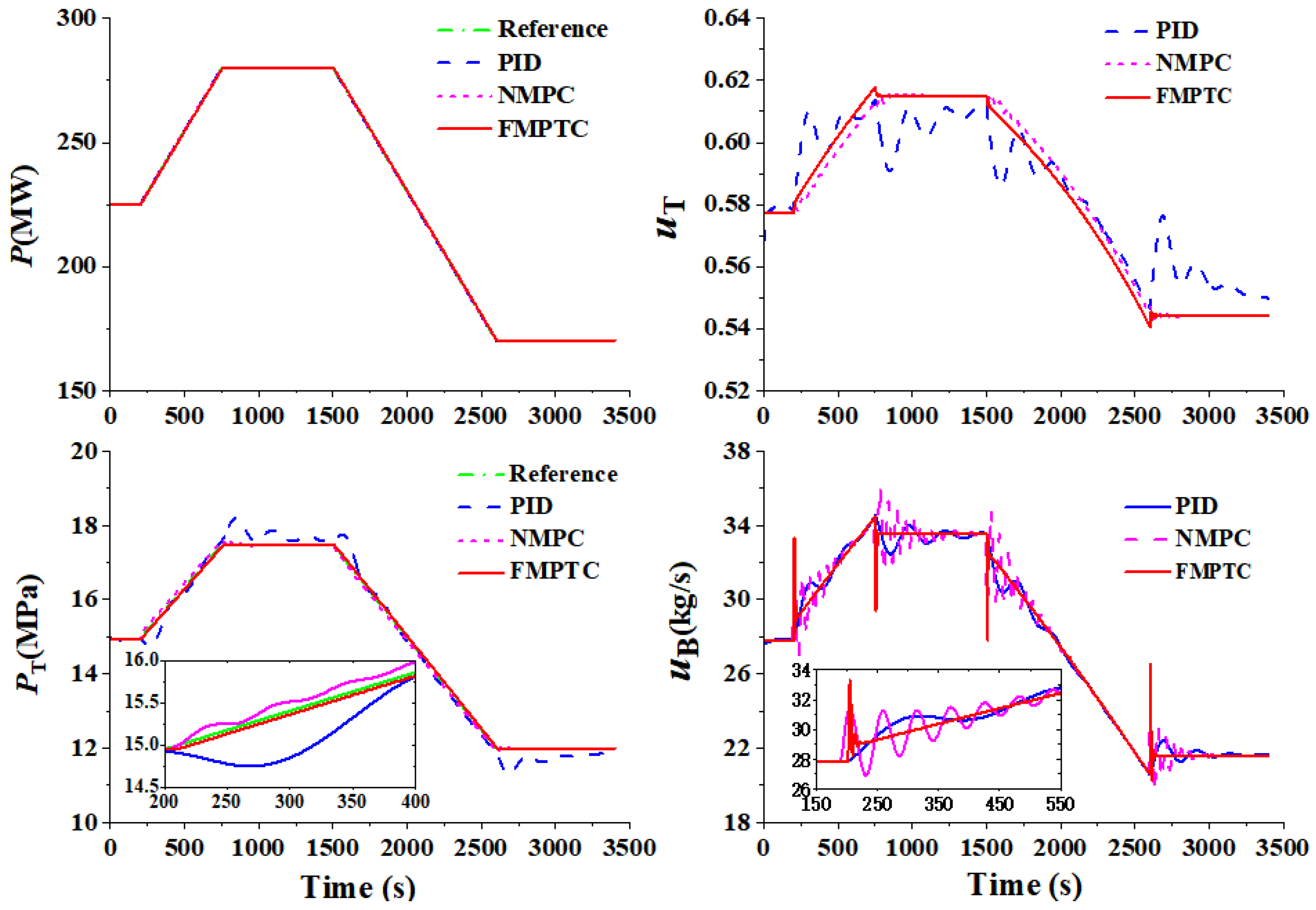
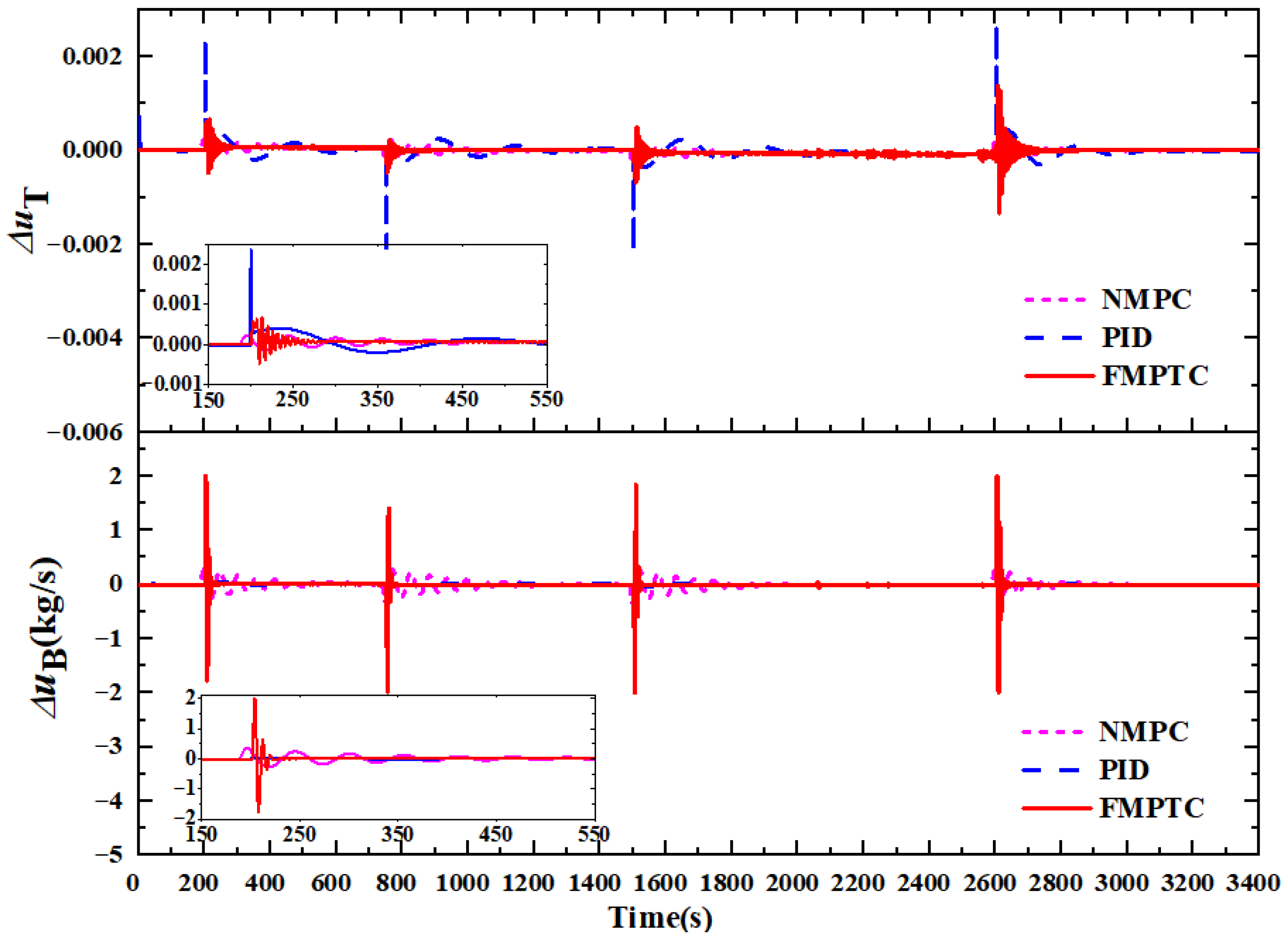
The simulation results are illustrated in Figure 4, and the root mean square errors (RMSEs) of the tracking performance for the three control schemes are summarized in

Table 1. RMSEs for the control schemes in Case 1.

	FMPTC	NMPC	PID
P (MW)	0.0313	0.0583	0.4193
PT (MPa)	0.0338	0.0655	0.2619

. It can be observed that the proposed FMPTC scheme nearly achieves ideal tracking of the power and throttle pressure set points over the wide operating range, with zero steady-state offset. Due to the strong nonlinearity induced by load variations and input constraints, the PID controller, well-tuned at the mid-range operating point (225 MW, 14.95 MPa), fails to deliver satisfactory performance across the full operating range. Regarding the NMPC scheme, which leverages the same fuzzy model as FMPTC instead of a single local linear model and incorporates constraints into the underlying optimization, its control performance over the wide operating range is significantly superior to that of the PID controller. However, NMPC exhibits slight inferiority to the FMPTC, as it produces a small overshoot when tracking the throttle pressure set point. Additionally, it is noteworthy that the stability of the NMPC-based closed-loop system is highly sensitive to the prediction and control horizons; improper tuning of these parameters may lead to system oscillation or even divergence. Figure 4 and Figure 5, respectively, present the control inputs and their increments. It can be observed that all three control schemes strictly comply with the predefined input constraints. This constraint satisfaction property holds for all subsequent simulation cases, where incremental control inputs are omitted for brevity.

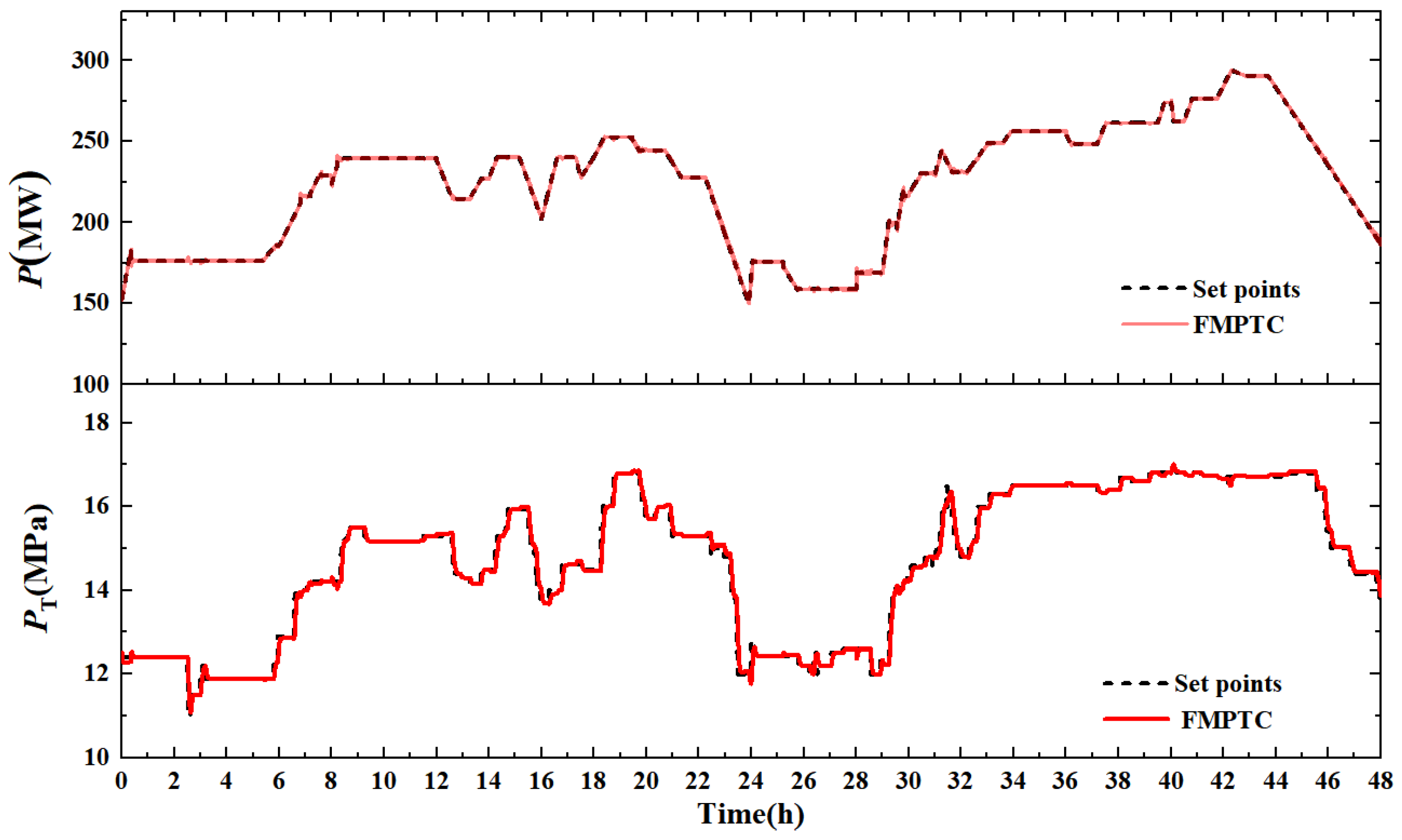
On the other hand, Figure 6 illustrates the tracking performance of the proposed FMPTC scheme with respect to the plant’s set points. It is evident that the output trajectories of the closed-loop system are nearly identical to the predefined set values. Consequently, the FMPTC scheme significantly outperforms the on-site PID controller adopted in practical power plant operations.

Case 2: Disturbance rejection

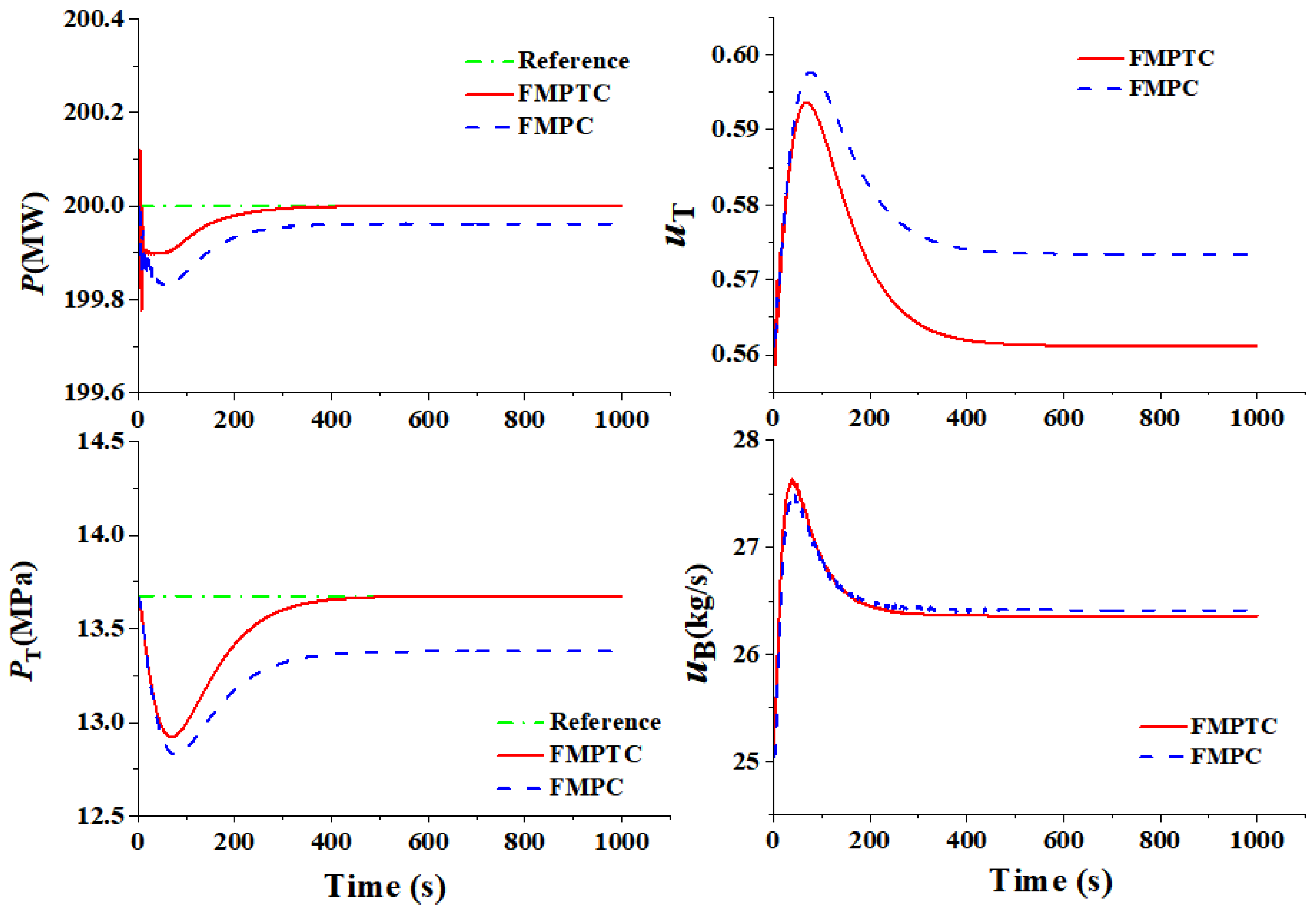
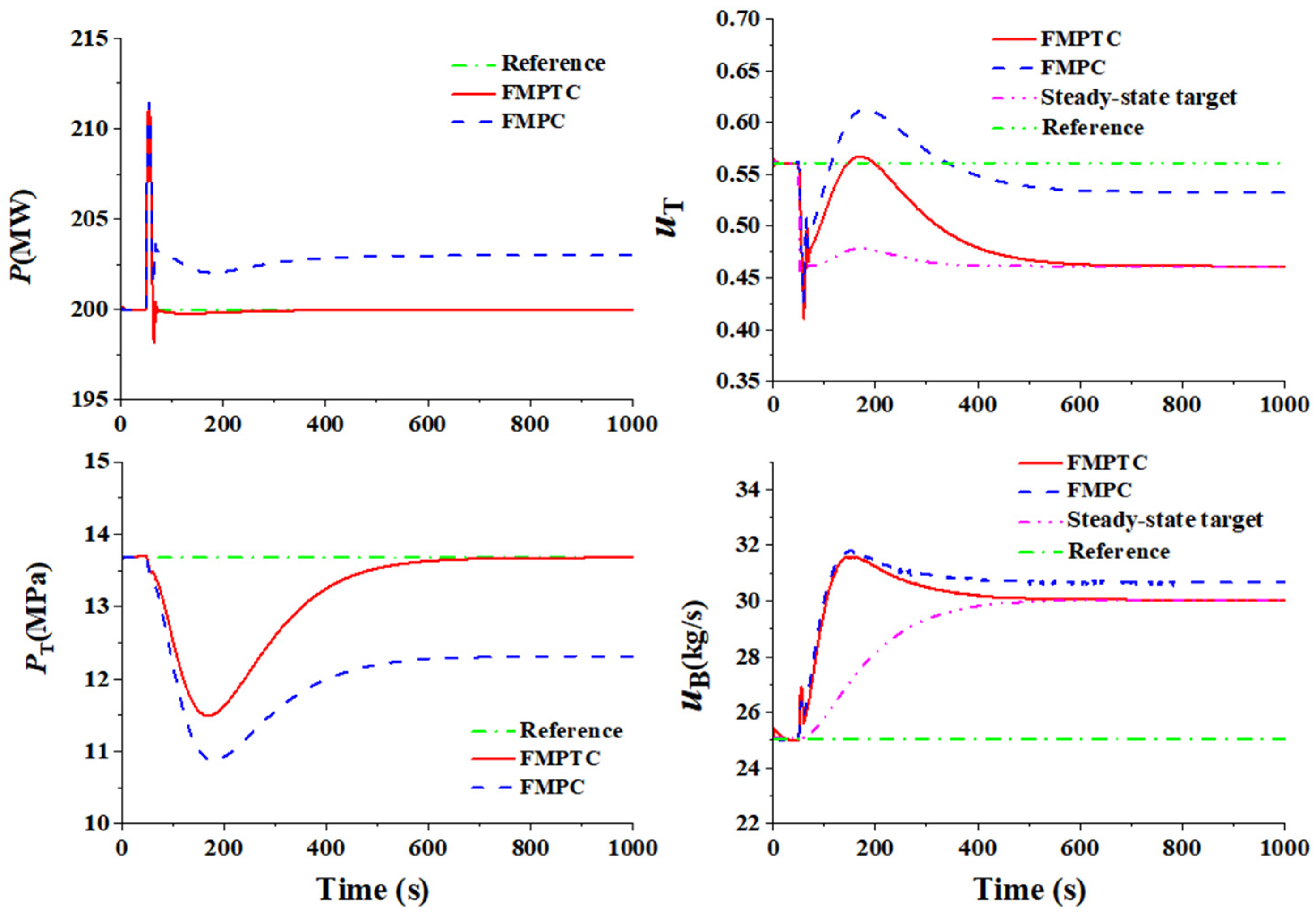
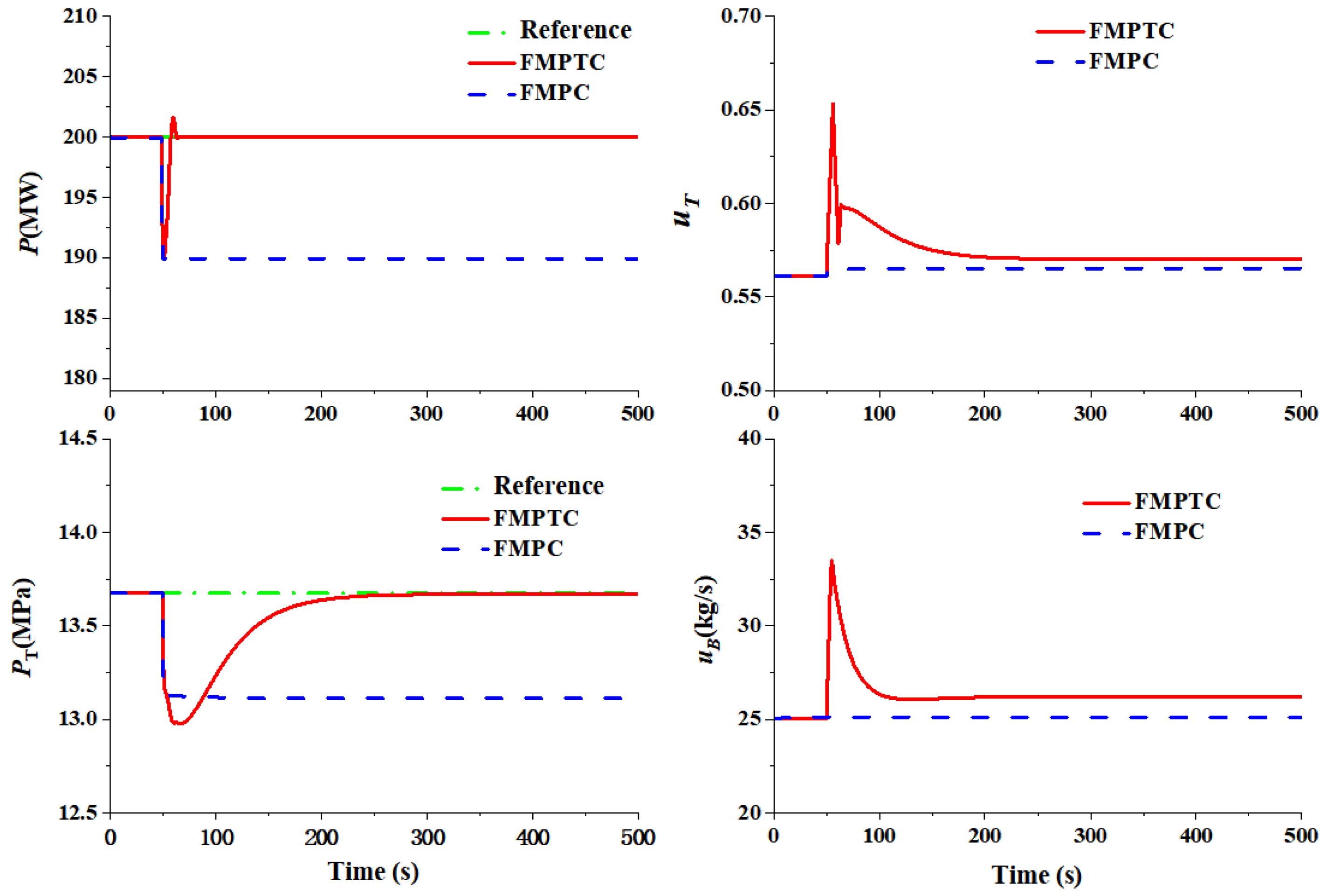
Next, a case is designed to verify the attenuation capability of the FMPTC scheme for the persistent disturbance, by comparing it with the FMPC scheme (i.e., the FMPTC framework without the SSTC module). In this scenario, the boiler-turbine system is assumed to operate at the nominal operating point (200 MW, 13.67 MPa). At t = 50 s, two unknown input disturbances d₁ = 0.1 (applied to the turbine valve opening u_T) and d₂ = −5 kg/s (applied to the fuel flow rate u_B) are introduced simultaneously.

The control performances of the two schemes are illustrated in Figure 7. It is evident that the FMPTC scheme can effectively mitigate the impact of input disturbances and drive the system back to the prescribed operating point with zero steady-state offset. In contrast, the FMPC scheme fails to cope with the disturbances, resulting in the system outputs settling at a new steady-state point deviating from the set values. The key distinction in control performance between FMPTC and FMPC lies in the SSTC module integrated into FMPTC: as depicted in Figure 7, the SSTC dynamically adjusts the steady-state targets online based on real-time disturbance estimates, thereby eliminating the adverse effects of disturbances on the controlled outputs.

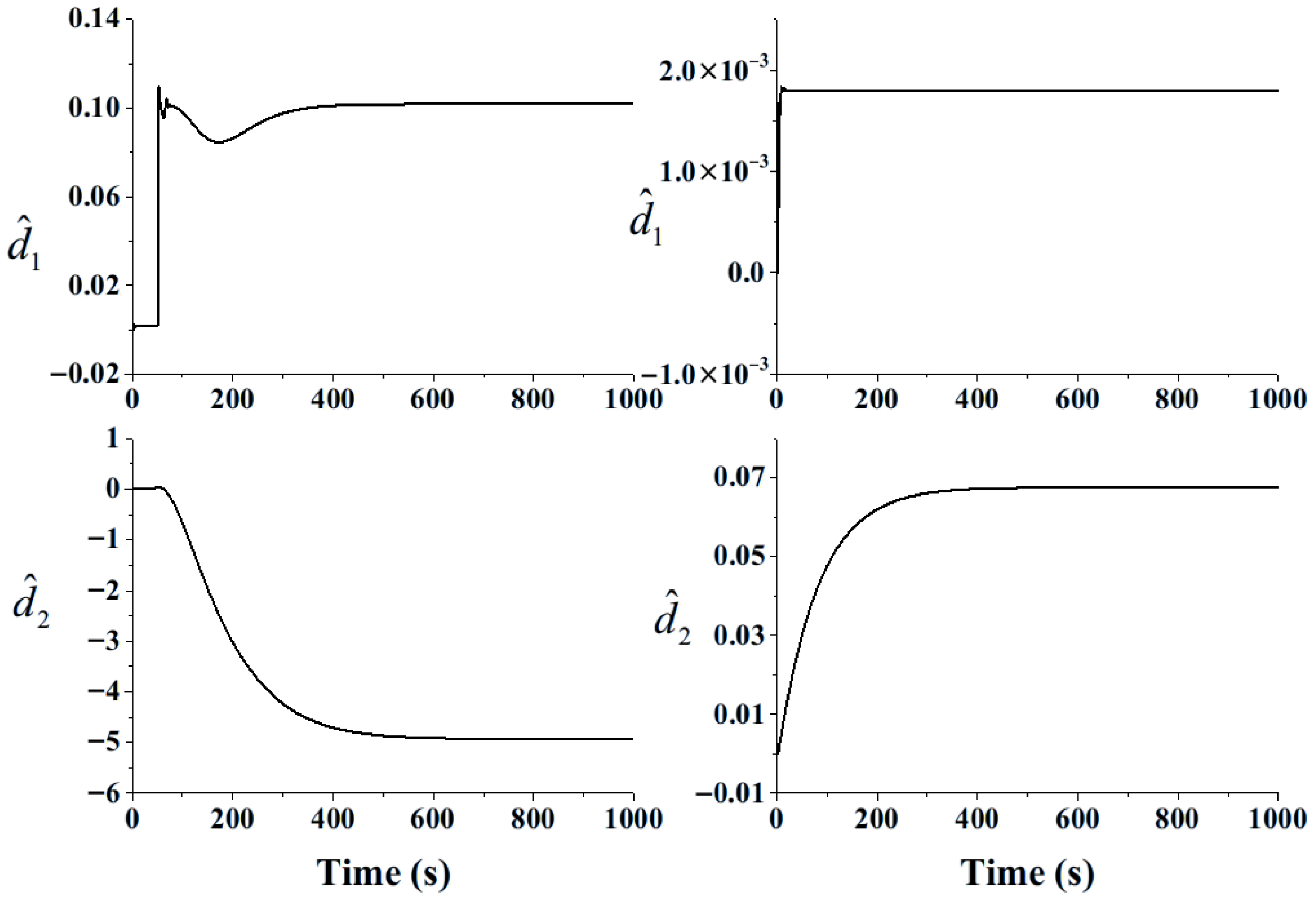
The two left subfigures of Figure 8 illustrate the estimates of the disturbance terms after input disturbances are imposed on the system. The two right subfigures present the estimates of the disturbance terms before any external disturbance is applied, where the observed disturbance terms only originate from the approximation error between the established T-S fuzzy model and the original nonlinear model of the boiler-turbine system. It can thus be inferred that the T-S fuzzy model exhibits high approximation accuracy for the nonlinear system, and the fuzzy extended state observer achieves satisfactory disturbance estimation performance. Note that the steady-state targets and disturbance estimates are presented in this case as illustrative examples; for brevity, they are not displayed in subsequent simulation cases.

The aforementioned subcase focuses on validating the scheme’s performance under input disturbances. Notably, the proposed control framework founded on the general disturbance model is equally effective for rejecting disturbances entering the system through other channels. Figure 9 gives the simulation result of the second subcase, in which at t = 50 s, two unknown output disturbances, p₁ = −10 MW (applied to the power output P) and p₂ = −0.5 MPa (applied to the throttle pressure P_T), are introduced. Additionally, Figure 10 illustrates the control performance under mixed disturbance conditions. Specifically, in this subcase, an unknown input disturbance d₁ = 0.1 (imposed on the turbine valve opening u_T) and an unknown output disturbance p₁ = −5 MW (imposed on the power output P) are applied simultaneously. Consistent with the observations from Figure 7, both Figure 9 and Figure 10 demonstrate the proposed control scheme’s strong disturbance rejection capability, confirming its effectiveness across input, output, and mixed disturbance scenarios.

Case 3: Robustness

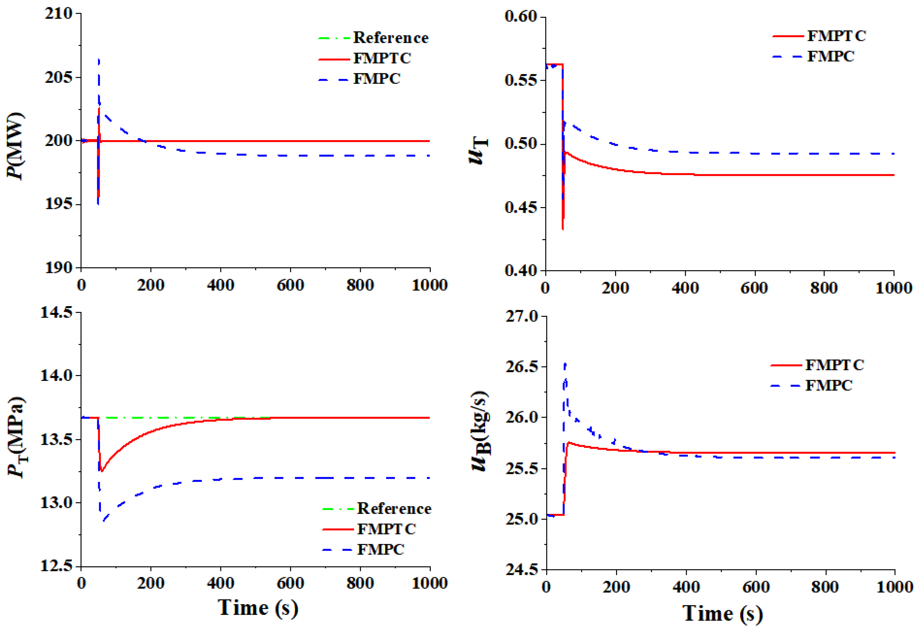
The final case is designed to evaluate the robustness of the proposed FMPTC scheme against model uncertainty. Specifically, this case considers a −5% variation in coal calorific value (corresponding to an approximate decrease of 1 MJ/kg). As indicated in the model parameter table of [37], the parameter k₄ (set to 20,237.25 in the nonlinear model (1)) exhibits a linear correlation with coal calorific value; thus, the aforementioned variation in coal calorific value will alter the nonlinear dynamics of the boiler-turbine system. The simulation results are illustrated in Figure 11. It is evident that the FMPTC scheme maintains strong robustness against the coal calorific value variation, ensuring the system outputs remain stable around the preset operating point. In contrast, the FMPC scheme fails to compensate for the model uncertainty induced by the coal calorific value change, leading to noticeable deviations of the output power and throttle pressure from the nominal operating point.

5. Conclusions

This paper proposes a fuzzy model predictive tracking control scheme for boiler-turbine systems subject to disturbances and input constraints. To comprehensively account for disturbance effects, the BTS is modelled using a GDM, which integrates two disturbance terms into the T-S fuzzy model to lump the combined impacts of unknown external disturbances and model uncertainty. The SSTC eliminates the adverse effects of disturbances on controlled variables by leveraging real-time disturbance estimates provided by FESO. The FMPTC scheme is formulated as an SDP problem. With the FMPTC, the closed-loop system is guaranteed to be asymptotically stable and tracks the set points without offset despite model uncertainty and external disturbances from any channel, and meanwhile, the input constraints on magnitude and change rate are satisfied by both the free control input and the future control inputs in the form of the non-PDC law. Case studies conducted on a 300 MW subcritical boiler-turbine unit validate the effectiveness and superiority of the proposed FMPTC scheme under various operating conditions.

References

1. Ye, J.; Pan, X.; Chen, G. The Principle and Equipment of Power Plant Boiler; China Power Press: Beijing, China, 2009; pp. 1–8. [Google Scholar]
2. Xu, L.; Yuan, J. Dynamic Modeling and Validation of the Boiler-Side Whole Process of Subcritical Coal-Fired Power Plants. In Proceedings of the Chinese Control Conference, Hangzhou, China, 28–30 July 2015; pp. 2093–2098. [Google Scholar] [CrossRef]
3. Tan, W.; Liu, J.; Fang, F.; Chen, Y. Tuning of PID Controllers for Boiler-Turbine Units. ISA Trans. 2004, 43, 571–583. [Google Scholar] [CrossRef]
4. Garrido, J.; Morilla, F.; Vazquez, F. Centralized PID Control by Decoupling of a Boiler-Turbine Unit. In Proceedings of the European Control Conference, Budapest, Hungary, 23–26 August 2009; pp. 4007–4012. [Google Scholar] [CrossRef]
5. Li, X.F.; Chen, G.; Wang, Y.G. IMC-PID Controller Design for Power Control Loop Based on Closed-Loop Identification in the Frequency Domain. IFAC Pap. 2016, 49, 79–84. [Google Scholar] [CrossRef]
6. Åstroöm, K.J.; Bell, R.D. Drum-Boiler Dynamics. Automatica 2000, 36, 363–378. [Google Scholar] [CrossRef]
7. Xu, L.; Yuan, J. Online Identification of the Lower Heating Value of the Coal Entering the Furnace Based on the Boiler-Side Whole Process Models. Fuel 2015, 161, 68–77. [Google Scholar] [CrossRef]
8. Nasiri, A.; Bayat, F.; Mobayen, S.; Hosseinnia, S.H. Gas Turbines Power Regulation Subject to Actuator Constraints, Disturbances and Measurement Noises. IEEE Access 2021, 9, 40155–40164. [Google Scholar] [CrossRef]
9. Moon, U.C.; Lee, K.Y. Step-Response Model Development for Dynamic Matrix Control of a Drum-Type Boiler–Turbine System. IEEE Trans. Energy Convers. 2009, 24, 423–430. [Google Scholar] [CrossRef]
10. Luo, J.; Zhu, Y.C.; Chen, S.H.; Jiang, P.F.; Xiao, Y.W. A Power Plant Coordinated Control System Using MPC. In Proceedings of the 2017 6th International Symposium on Advanced Control of Industrial Processes (AdCONIP), Taipei, Taiwan, 28–31 May 2017; pp. 336–341. [Google Scholar] [CrossRef]
11. Karampoorian, H.R.; Mohseni, R. Generalized Model Predictive Control for a Multivariable Boiler-Turbine Unit. In Proceedings of the 11th International Conference on Control, Automation and Systems (ICCAS), Gyeonggi-do, Republic of Korea, 26–29 October 2011; pp. 811–814. [Google Scholar]
12. Zhang, F.; Shen, J.; Li, Y.; Wu, X. Nonlinear Model Predictive Control of Ultra-Supercritical Once through Boiler-Turbine Unit. In Proceedings of the Chinese Automation Conference (CAC), Wuhan, China, 27–29 November 2015; pp. 2194–2198. [Google Scholar] [CrossRef]
13. Kong, X.; Liu, X.; Lee, K.Y. An Effective Nonlinear Multivariable HMPC for USC Power Plant Incorporating NFN-Based Modeling. IEEE Trans. Ind. Inform. 2016, 12, 555–566. [Google Scholar] [CrossRef]
14. Sarailoo, M.; Rahmani, Z.; Rezaie, B. Fuzzy Predictive Control of a Boiler–Turbine System Based on a Hybrid Model System. Ind. Eng. Chem. Res. 2014, 53, 2362–2381. [Google Scholar] [CrossRef]
15. Ławryńczuk, M. Nonlinear Predictive Control of a Boiler-Turbine Unit: A State-Space Approach with Successive On-Line Model Linearisation and Quadratic Optimisation. ISA Trans. 2017, 67, 476–495. [Google Scholar] [CrossRef]
16. Zhang, F.; Wu, X.; Shen, J. Extended State Observer Based Fuzzy Model Predictive Control for Ultra-Supercritical Boiler-Turbine Unit. Appl. Therm. Eng. 2017, 118, 90–100. [Google Scholar] [CrossRef]
17. Zhu, J. Nonlinear Dynamic Investigation and Anti-Bifurcation Control of a Boiler-Turbine Unit via Dual-Mode Fuzzy Model Predictive Control Strategy. J. Frankl. Inst. 2021, 358, 7365–7393. [Google Scholar] [CrossRef]
18. Wu, X.; Shen, J.; Li, Y.; Lee, K.Y. Fuzzy Modeling and Stable Model Predictive Tracking Control of Large-Scale Power Plants. J. Process Control 2014, 24, 1609–1626. [Google Scholar] [CrossRef]
19. Takagi, T.; Sugeno, M. Fuzzy Identification of Systems and Its Applications to Modeling and Control. IEEE Trans. Syst. Man Cybern. 1985, SMC-15, 116–132. [Google Scholar] [CrossRef]
20. Feng, G. A Survey on Analysis and Design of Model-Based Fuzzy Control Systems. IEEE Trans. Fuzzy Syst. 2006, 14, 676–697. [Google Scholar] [CrossRef]
21. Cheng, L.; Liu, W.; Hou, Z.G.; Huang, T.; Yu, J.; Tan, M. An Adaptive Takagi–Sugeno Fuzzy Model-Based Predictive Controller for Piezoelectric Actuators. IEEE Trans. Ind. Electron. 2017, 64, 3048–3058. [Google Scholar] [CrossRef]
22. Kong, L.; Yuan, J. Disturbance-Observer-Based Fuzzy Model Predictive Control for Nonlinear Processes with Disturbances and Input Constraints. ISA Trans. 2019, 90, 89–106. [Google Scholar] [CrossRef]
23. Kong, L.; Yuan, J. Generalized Discrete-Time Nonlinear Disturbance Observer Based Fuzzy Model Predictive Control for Boiler-Turbine Systems. ISA Trans. 2019, 90, 74–88. [Google Scholar] [CrossRef] [PubMed]
24. Qin, S.J.; Badgwell, T.A. A Survey of Industrial Model Predictive Control Technology. Control Eng. Pract. 2003, 11, 733–764. [Google Scholar] [CrossRef]
25. Aydin, B.E.; Van Overloop, P.J.; Rutten, M.; Tian, X. Offset-Free Model Predictive Control of an Open Water Channel Based on Moving Horizon Estimation. J. Irrig. Drain. Eng. 2016, 143, B4016005. [Google Scholar] [CrossRef]
26. Horváth, K.; Galvis, E.; Valentín, M.G.; Rodellar, J. New Offset-Free Method for Model Predictive Control of Open Channels. Control Eng. Pract. 2015, 41, 13–25. [Google Scholar] [CrossRef]
27. Muske, K.R.; Badgwell, T.A. Disturbance Modeling for Offset-Free Linear Model Predictive Control. J. Process Control 2002, 12, 617–632. [Google Scholar] [CrossRef]
28. Pannocchia, G.; Rawlings, J.B. Disturbance Models for Offset-Free MPC Control. Aiche J. 2010, 49, 426–437. [Google Scholar] [CrossRef]
29. Borrelli, F.; Morari, M. Offset free model predictive control. In Proceedings of the 46th IEEE Conference on Decision and Control, New Orleans, LA, USA, 12–14 December 2007; pp. 1245–1250. [Google Scholar] [CrossRef]
30. Maeder, U.; Borrelli, F.; Morari, M. Linear Offset-Free Model Predictive Control. Automatica 2009, 45, 2214–2222. [Google Scholar] [CrossRef]
31. Maeder, U.; Morari, M. Offset-Free Reference Tracking with Model Predictive Control. Automatica 2010, 46, 1469–1476. [Google Scholar] [CrossRef]
32. Wallace, M.; Das, B.; Mhaskar, P.; House, J.; Salsbury, T. Offset-Free Model Predictive Control of a Vapor Compression Cycle. J. Process Control 2012, 22, 1374–1386. [Google Scholar] [CrossRef]
33. Wang, H.; Zhao, J.; Xu, Z.; Shao, Z. Linear Offset-Free Model Predictive Control: A Minimum-Variance Unbiased Filter Based Approach. In Proceedings of the 52nd IEEE Conference on Decision and Control, Florence, Italy, 10–13 December 2013; pp. 782–786. [Google Scholar] [CrossRef]
34. Aydn, B.E.; Overloop, P.J.V.; Tian, X. Offset free model predictive control of an open water reach. In Proceedings of the International Conference on Hydroinformatics, New York, NY, USA, 17–24 August 2014; pp. 301–307. [Google Scholar]
35. Yaghini, H.H.; Bagheri, P.; Kharrati, H. Observer-Based Offset-Free Model Predictive Control for Fractional-Order Systems. Int. J. Dyn. Control 2024, 12, 1942–1951. [Google Scholar] [CrossRef]
36. Eni, O.; Wang, M. Dynamic Modelling, Validation and Analysis of Coal-Fired Subcritical Power Plant. Fuel 2014, 135, 292–300. [Google Scholar] [CrossRef]
37. Tian, Z.; Yuan, J.; Xu, L. Modeling of Drum Boiler-Turbine Unit and the Model-Based Coordinated Control Strategy. In Proceedings of the 35th Chinese Control Conference (CCC), Chengdu, China, 27–29 July 2016; pp. 3327–3332. [Google Scholar] [CrossRef]
38. Biglarbegian, M.; Sadeghian, A.; Melek, W. On the Accessibility/Controllability of Fuzzy Control Systems. Inf. Sci. 2012, 202, 58–72. [Google Scholar] [CrossRef]
39. Kong, L.; Yuan, J. New Relaxed Stabilization Conditions for Discrete-Time Takagi–Sugeno Fuzzy Control Systems. Asian J. Control 2020, 22, 1604–1616. [Google Scholar] [CrossRef]
40. Kothare, M.V.; Morari, M.; Balakrishnan, V. Robust constrained model predictive control using linear matrix inequalities. Automatica 1996, 32, 1361–1379. [Google Scholar] [CrossRef]
41. Lu, Y.; Arkun, Y. Quasi-Min-Max MPC Algorithms for LPV Systems. Automatica 2000, 36, 527–540. [Google Scholar] [CrossRef]
42. Ding, B.; Xi, Y.; Li, S. A Synthesis Approach of On-Line Constrained Robust Model Predictive Control. Automatica 2004, 40, 163–167. [Google Scholar] [CrossRef]
43. Ding, B. Stabilization of Takagi–Sugeno Model via Nonparallel Distributed Compensation Law. IEEE Trans. Fuzzy Syst. 2010, 18, 188–194. [Google Scholar] [CrossRef]
44. Sun, L. DEB-Oriented Modelling and Control of Coal-Fired Power Plant. IFAC Proc. Vol. 2014, 47, 413–418. [Google Scholar] [CrossRef]
45. Xi, Y. Predictive Control, 2nd ed.; National Defense Industry Press: Beijing, China, 2012; pp. 130–156. [Google Scholar]
46. Wachter, A.; Biegler, L.T. On the Implementation of an Interior-Point Filter Line-Search Algorithm for Large-Scale Nonlinear Programming. Math. Program 2006, 106, 25–57. [Google Scholar] [CrossRef]
47. Guerra, T.M.; Vermeiren, L. LMI-Based Relaxed Nonquadratic Stabilization Conditions for Nonlinear Systems in the Takagi–Sugeno’s Form. Automatica 2004, 40, 823–829. [Google Scholar] [CrossRef]
Figure 1. Schematic description of the subcritical boiler-turbine system (HPC: high-pressure cylinder, LPC: low-pressure cylinder, RES: regenerative extraction system).
Mathematics 13 03755 g001
Figure 2. Membership functions of the fuzzy sets.
Mathematics 13 03755 g002
Figure 3. The proposed FMPTC scheme for the BTS.
Mathematics 13 03755 g003
Figure 4. Performance of the BTS for a ramp-type load variation: 225-280-170 MW.
Mathematics 13 03755 g004
Figure 5. Incremental control inputs of the BTS for a ramp-type load variation: 225-280-170 MW.
Mathematics 13 03755 g005
Figure 6. Tracking performance of FMPTC for the plant set points of the BTS.
Mathematics 13 03755 g006
Figure 7. Performance of the BTS with unknown input disturbances.
Mathematics 13 03755 g007
Figure 8. Estimates of the disturbance terms for FMPTC: (left) with the input disturbances; (right) without the input disturbances.
Mathematics 13 03755 g008
Figure 9. Performance of the BTS with unknown output disturbances.
Mathematics 13 03755 g009
Figure 10. Performance of the BTS with unknown mixed disturbances.
Mathematics 13 03755 g010
Figure 11. Performance of the BTS with the model uncertainty.
Mathematics 13 03755 g011