Scalable QR Factorisation of Ill-Conditioned Tall-and-Skinny Matrices on Distributed GPU Systems

Abstract

The QR factorisation is a cornerstone of numerical linear algebra, essential for solving overdetermined linear systems, eigenvalue problems, and various scientific computing tasks. However, computing it for ill-conditioned tall-and-skinny (TS) matrices on large-scale distributed-memory systems, particularly those with multiple GPUs, presents significant challenges in balancing numerical stability, high performance, and efficient communication. Traditional Householder-based QR methods provide numerical stability but perform poorly on TS matrices due to their reliance on memory-bound kernels. This paper introduces a novel algorithm for computing the QR factorisation of ill-conditioned TS matrices based on CholeskyQR methods. Although CholeskyQR is fast, it typically fails due to severe loss of orthogonality for ill-conditioned inputs. To solve this, our new algorithm, mCQRGSI+, combines the speed of CholeskyQR with stabilising techniques from the Gram–Schmidt process. It is specifically optimised for distributed multi-GPU systems, using adaptive strategies to balance computation and communication. Our analysis shows the method achieves accuracy comparable to Householder QR, even for extremely ill-conditioned matrices (condition numbers up to ${10}^{16}$). Scaling experiments demonstrate speedups of up to $12\times$ over ScaLAPACK and $16\times$ over SLATE’s CholeskyQR2. This work delivers a method that is both robust and highly parallel, advancing the state-of-the-art for this challenging class of problems.

1. Introduction

The introduction of heterogeneous architectures into high-performance computing has driven advancements in linear algebra, leading to the redesign of its core algorithms to meet the requirement for an increased level of parallelism [1]. Simultaneously, a trend towards task-based parallelism and the use of dynamic runtime systems emerged with the aim of managing the complexity of distributed, heterogeneous hardware [2,3]. Apart from the advanced runtime development, the design of numerical algorithms tailored for distributed heterogeneous architectures remains critical. In this paper, we focus on the QR factorisation [4] and its implementations tailored to large distributed-memory systems. In its basic form, the QR factorisation of a rectangular matrix $A\in {\mathbb{R}}^{m\times n}$, $m\ge n$, is

$$A=QR,$$

(1)

where $Q\in R^{m\times n}$ is an orthogonal matrix and $R\in {\mathbb{R}}^{n\times n}$ is an upper triangular matrix. Finding the QR decomposition of large rectangular matrices is a crucial step in various numerical methods, such as block methods (e.g., in the solution of linear systems with multiple right-hand sides [5]), Krylov subspace methods [6], eigenvalue solvers (e.g., in the reduction to band form in multi-stage eigensolvers [7]), subspace iteration [8], and solving dense least squares problems for overdetermined systems. In some extreme cases, where $m\gg n$, i.e., the matrix has many more rows than columns, a so-called tall-and-skinny (TS) matrix, the calculation of the QR factorisation becomes a critical path and requires special methods. One example is a subspace projection iterative eigensolver [8] to calculate a small fraction of the extreme eigenvalues.

The most stable and accurate method for computing the QR factorisation of general matrices is based on Householder reflectors [4], commonly known as Householder QR. The algorithm determines a set of orthogonal Householder matrices that annihilate the entries below the main diagonal of A column by column, while the rest of the matrix is updated (trailing update). This type of algorithm, in which R is formed by applying an orthogonal matrix from the left, $Q^{T}A=R$, is called orthogonal triangularisation and provides good numerical stability. Highly efficient implementations that factorise blocks or panels of columns are available in many numerical libraries, such as ScaLAPACK [9] for distributed memory systems and MAGMA [10] for heterogeneous and accelerator-based shared memory systems. However, Householder QR cannot achieve high performance for tall-and-skinny matrices [11] because panel factorisation with many more rows than columns relies on much slower Level-1 and Level-2 BLAS kernels, which cannot be compensated by the highly parallel and optimised Level-3 BLAS kernels used in the trailing update [12].

To avoid working with very tall-and-skinny panels, the Tall–Skinny QR (TSQR) algorithm [11,13] was developed. TSQR offers improved parallelisation on distributed memory systems and reduces communication. The main idea is to split the input matrix into a one-dimensional block row layout, allowing QR factorisations to be performed concurrently on local blocks. In subsequent reduction steps, the intermediate R-factors are grouped into pairs and orthogonalised. This process is repeated until the final upper triangular R is obtained. Although the degree of parallelism is significantly increased compared to traditional Householder QR, a large number of flops are still performed in memory-bound Level-1 and Level-2 BLAS kernels to orthogonalise the local blocks. The distributed version of TSQR is implemented in the SLATE library [14] as part of the Communication Avoiding QR (CAQR) algorithm, where it is used for QR factorisation of tall-and-skinny panels. CAQR was developed for general matrices, not specifically for TS matrices. It is more efficient than the standard distributed QR, as it reduces the communication volume.

An alternative approach to compute the QR factorisation of a full column-ranked matrix A is the Gram–Schmidt algorithm [4], particularly its block variants, which offer performance advantages. The block classical Gram–Schmidt algorithm achieves better parallel performance than the modified version due to fewer synchronisation points, but it suffers from severe loss of orthogonality. The modified Gram–Schmidt algorithm significantly reduces this loss (upper bounded by $\mathcal{O}\left(ϵ\right)\kappa \left(A\right)$) [15], but it is still outperformed in terms of stability by Householder-based QR, whose loss of orthogonality is $\mathcal{O}\left(ϵ\right)$. The performance and stability of Gram–Schmidt depend on the algorithm chosen for inner orthogonalisation, for which various implementations are available. An excellent overview and stability analysis of different combinations of Gram–Schmidt variants with inner orthogonalisation algorithms can be found in [16].

This work highlights the central challenge for ill-conditioned matrices: balancing performance and numerical stability. This paper addresses this trade-off directly, presenting an approach in which, for $\kappa \left(A\right)\mathcal{O}\left(ϵ\right)<1$, the loss of orthogonality remains at $\mathcal{O}\left(ϵ\right)$. To address this challenge, we present a novel algorithm for computing the QR factorisation of ill-conditioned tall-and-skinny matrices, which combines block modified Gram–Schmidt orthogonalisation with the CholeskyQR algorithm as a local panel reorthogonalisation. A key innovation of this work is an algorithm specifically optimised for distributed memory GPU systems. To the best of our knowledge, this is the first QR factorisation algorithm designed for this class of matrices on such architectures. The resulting method achieves orthogonality and numerical stability comparable to those of Householder-based QR factorisation algorithms. Consequently, our algorithm outperforms other methods, including the Shifted CholeskyQR3 algorithm and traditional Householder-based approaches such as ScaLAPACK’s PDGEQRF. To situate this work, we also provide a detailed analysis and synthesis of the state-of-the-art in CholeskyQR-based QR factorisation algorithms for tall-and-skinny matrices.

The original scientific contributions in this paper are as follows:

• Novel algorithm for computing the QR factorisation (mCQRGSI+) of ill-conditioned tall-and-skinny matrices.
• The proposed algorithm maintains high orthogonality and numerical robustness for ill-conditioned matrices.
• Delivering efficient performance on distributed GPU systems.

The rest of the paper is organised as follows. Section 2 provides an overview of state-of-the-art methods based on the CholeskyQR method for computing the QR factorisation of very ill-conditioned matrices. The benchmarking environment, input matrix dataset and competitive libraries used in the performance analysis are described in Section 3. Section 4 introduces CholeskyQR2 with block Gram–Schmidt, tailored for distributed multi-GPU systems, together with a stability and performance analysis. Building on the same parallelisation patterns, Section 5 presents our novel algorithm that combines block Gram–Schmidt with CholeskyQR for inter-reorthogonalisation. Detailed performance analysis, including strong and weak scalability, is reported in Section 6. Finally, Section 7 concludes the paper by summarising the main results and outlining directions for future work.

2. QR Factorisation Based on CholeskyQR

In our research, we explore alternative methods for computing the QR factorisation of ill-conditioned, tall-and-skinny matrices, based on the CholeskyQR algorithm. CholeskyQR (CQR) is a simple algorithm with very low communication overhead and approximately half the arithmetic cost of TSQR [4]. The algorithm involves constructing a Gram matrix (based completely on matrix multiplication), performing Cholesky factorisation, and a symmetric rank-k update to construct the factor Q ($Q=A{R}^{-1}$). For further details, see, for example, Algorithm 1 in [17]. The advantage is that all steps can be implemented as level-3 BLAS operations and require only one synchronisation point, which ensures significantly better performance on large parallel systems. The main drawback is that the algorithm is numerically unstable. The loss of orthogonality increases with the condition number of the input matrix A and is upper bounded by $\mathcal{O}\left(ϵ\right){\kappa }^2\left(A\right)$ [18], where $ϵ$ is the machine precision. Since the matrix multiplication squares the condition number, the resulting Gram matrix may not be positive definite for very ill-conditioned matrices, causing the Cholesky factorisation step to fail.

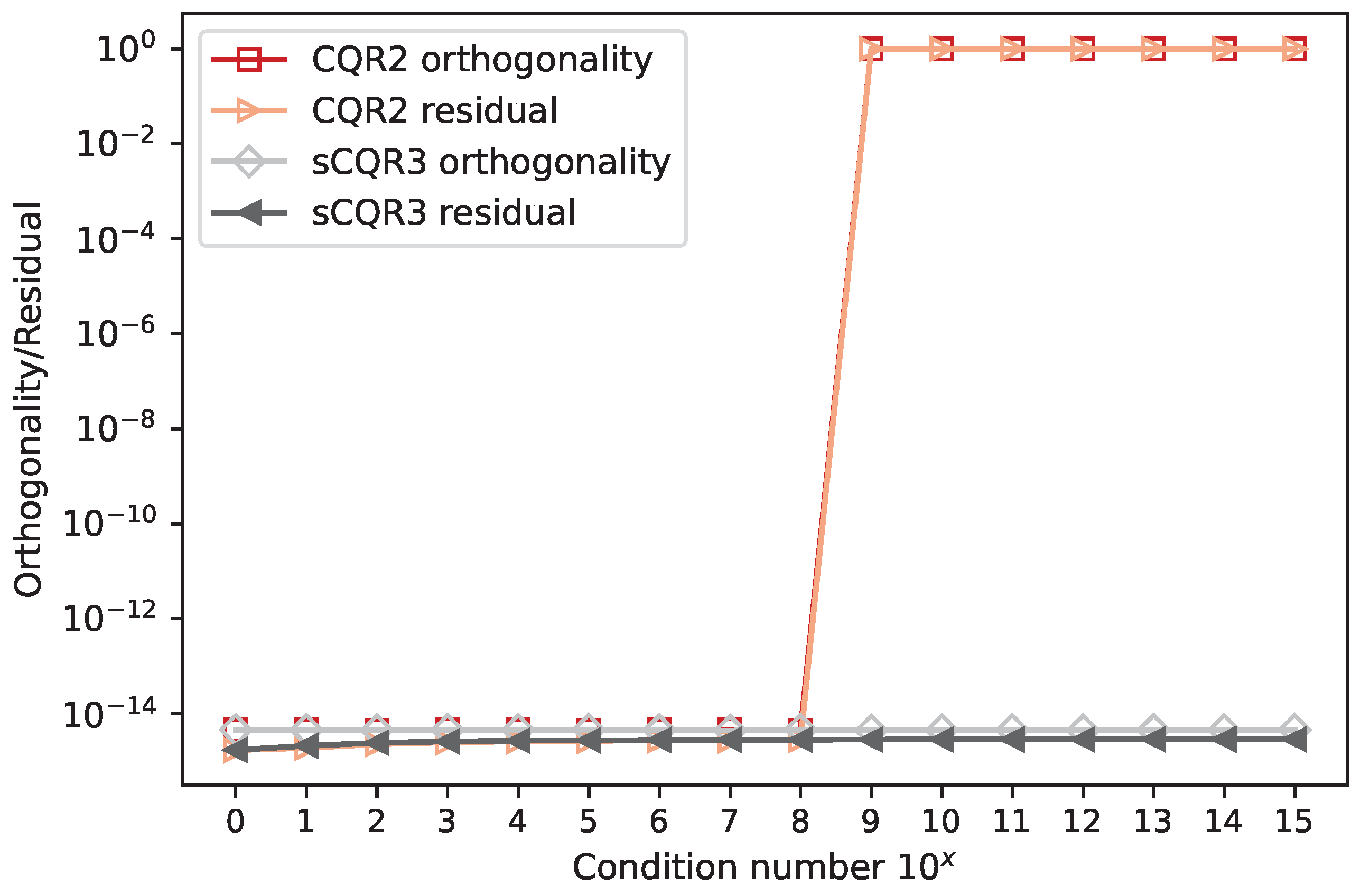
The idea of improving orthogonality by iteratively applying an algorithm was first proposed in [18]. Based on this idea, the authors in [19,20] proposed an algorithm called CholeskyQR2 (CQR2), which repeats the CholeskyQR algorithm twice. When applied twice, the algorithm achieves accuracy and loss of orthogonality comparable to TSQR but also requires twice as much communication as CholeskyQR, with an arithmetic cost equivalent to that of TSQR. Although the loss of orthogonality is significantly improved, this holds only if the condition number satisfies $\mathcal{O}\left(ϵ\right){\kappa }^2\left(A\right)<1$. In practice, in double precision arithmetic for matrices with condition numbers $\kappa \left(A\right)\gg {10}^8$, the algorithm fails to produce an orthogonal matrix [19,20]; see Figure 1.

Figure 1. Orthogonality and residuals of sCQR3 and CQR2 as a function of the condition number, for input matrices with m = 30,000, $n=3000$ and conservative shift for sCQR3.

This issue is addressed by the Shifted CholeskyQR algorithm [18,21]. The idea is to construct a shifted Gram matrix $\widehat{W}:=A^{T}A+\sigma I$, where the shift factor $\sigma$ ensures the numerical stability of the subsequent Cholesky factorisation. The proposed algorithm, referred to as Shifted CholeskyQR3 (sCQR), uses Shifted CholeskyQR as a preconditioner for CholeskyQR2. This increases the computational cost by $50\%$ compared to CholeskyQR2, making Shifted CholeskyQR3 inferior in terms of performance. In practice, the choice of using shift can be decided at runtime and thus decrease the computational cost. With a well-chosen shift, the algorithm is suitable for matrices with condition numbers up to $\mathcal{O}\left({ϵ}^{-1}\right)$. In our research, we adopted the conservative approach (as proposed in [22]), where the Frobenius norm is used to calculate the shift factor, ensuring numerical stability (see Figure 1) with fewer flops.

Other approaches to improve the applicability of CholeskyQR for ill-conditioned matrices have also been explored. In [23], the LU decomposition is used as a precondition for Cholesky factorisation [23]. After an initial LU decomposition ($PA:=LU$), the standard CholeskyQR2 can be applied to the matrix $L^{T}L$, since L is usually better conditioned than A. The achieved orthogonality and residual are comparable to Householder QR, even for very ill-conditioned matrices, when $\kappa \left(A\right)>{ϵ}^{-1/2}$. The algorithm exhibits less parallelism because of partial pivoting in LU and is approximately $1.5\times$ slower on shared memory systems and between $3\times$ and $5\times$ slower on distributed memory systems than CholeskyQR2.

More recent improvements include randomised Householder–Cholesky QR factorisation with multisketching [24]. This approach applies up to two randomised sketch matrices (multisketching), which ensure that the orthogonality error is bounded by a constant of the order of unit roundoff for matrices of arbitrary condition number. The first step is to compute the randomised Householder QR that generates the matrix $Q_1$ orthogonal to the given sketch matrices. As in other similar approaches, the obtained matrix is reorthogonalised in the second step by applying CholeskyQR2 to produce a fully orthogonal matrix Q. The algorithm applies to extremely tall-and-skinny matrices ($n\le 0.01\%m$), and is only negligibly faster than CholeskyQR2, but is more stable than Shifted CholeskyQR3.

Another approach, randomised CholeskyQR presented in [25], proposes computing the R factor from a small random sketch of X instead of $X^{T}X$, reducing computational cost and improving numerical stability. This randomised CholeskyQR variant uses half the flops of the classical CholeskyQR method, maintains the same communication cost, and remains stable for numerically full-rank matrices. However, when an orthonormal matrix Q is needed, randomised CholeskyQR must typically be augmented with an additional classical CholeskyQR step, thereby increasing the computational cost and diminishing the overall advantage of the method.

Since the orthogonality error of CholeskyQR depends quadratically on the condition number, the authors in [26] have proposed a mixed-precision approach. In this approach, the input and output matrices are retained in their required precision, while certain intermediate results are calculated in higher precision. The analysis has shown that the orthogonality error of the mixed-precision CholeskyQR approach has a linear dependence on the condition number of the input matrix when double precision is used. The main drawback of the proposed algorithm is that the number of floating-point instructions increases significantly when double precision is used (especially when the target precision is 64-bit).

Finally, the stability of Cholesky decomposition can be restored by combining CholeskyQR with Gram–Schmidt reorthogonalisation [27]. The proposed algorithm has shown that the resulting orthogonality is equivalent to that of Householder-based QR factorisations (general and TSQR), but it cannot exploit massively parallel systems as the method uses very tall-and-skinny column panels with full column size. This method served as the foundation for the work presented in this paper.

3. Testing Environment

The empirical evaluation of the numerical stability and performance of the codes was conducted on the Supek supercomputer at the University Computing Centre (SRCE), University of Zagreb. The tests were performed on two partitions: GPU and CPU. The GPU partition consists of 20 nodes interconnected with the Cray Slingshot. Each node has an AMD EPYC 7763 CPU with 64 cores and 512 GB of main memory, supported by four NVIDIA A100 Tensor Core GPUs with 40 GB of device memory each. The CPU partition consists of 52 nodes similar to the GPU partition, but with 2 AMD EPYC processors (128 cores in total) and without GPU accelerators. All codes were compiled with CMake 3.26.0 using gcc 11.2.1, CUDA 12.5, Intel oneAPI MKL 2023.1.0, Cray-MPICH 8.1.26 and Nvidia NCCL 2.18.5 for node-to-node communication.

To systematically study the effects of ill-conditioning, the input data are artificially generated matrices with a condition number $\kappa \left(A\right)$ in the range $\{{10}^0,{10}^1,\dots ,{10}^{15}\}$. The matrices are generated using the singular vector decomposition (SVD) ($U\Sigma V$), where U and V are the left and right singular vector matrices obtained from the SVD of a random input matrix. The new diagonal matrix $\Sigma$ is constructed with diagonal elements $(1,{\sigma }^{{\displaystyle \frac{1}{n-1}}},\dots ,{\sigma }^{{\displaystyle \frac{n-2}{n-1}}},\sigma )$. The parameter $\sigma$ controls the condition number of the generated matrix A, i.e., $\kappa \left(A\right)\approx \sigma$. For the numerical stability tests, we used matrices of size $\mathrm{30,000}\times 3000$ and the full condition number range in double precision.

Numerical accuracy is assessed by analysing the loss of orthogonality of the computed factor Q using the formula $\parallel Q^T{Q-I\parallel }_F/\sqrt{n}$, where I is the identity matrix, and the residual ${\parallel QR-A\parallel }_F/{\parallel A\parallel }_F$. Both the loss of orthogonality and the residual should be of the order $\mathcal{O}\left(ϵ\right)$, where $ϵ$ is the machine precision of a certain numerical type. In our experiments, all computational routines were performed strictly in double-precision arithmetic, and the average execution time of 10 runs is reported for each experiment. The standard deviation of the execution times in all of our cases was two to three orders of magnitude smaller than the mean, which can be considered negligible.

Performance was evaluated through both strong and weak scaling tests. The strong scaling tests were performed for matrices with 120,000 rows and the number of columns equal to $1\%$, $5\%$ and $10\%$ of the number of rows. The weak scalability analysis was performed on matrices with 40k, 80k, 120k, …, 480k rows and the number of columns fixed at 3000, resulting in blocks of size 10k × 3k per process (MPI or NCCL rank). The code supports both CPU-only and hybrid CPU-GPU execution. Unless otherwise explicitly stated, all tests were performed on GPUs with the suffix MPI or NCCL, denoting whether the MPI or NCCL library was used.

The results are compared to the SLATE (Software for Linear Algebra Targeting Exascale) library implementation of CholeskyQR2 [14]. To the best of our knowledge, SLATE is the only numerical linear algebra library that implements distributed GPU versions of various QR decomposition algorithms, including the basic CholeskyQR. In this work, the CholeskyQR2 implementation was achieved by invoking the cholqr function twice. In the experiments, SLATE version 2024.10.29, obtained from the official GitHub repository https://github.com/icl-utk-edu/slate (accessed on 15 May 2025) was used, including all code changes present in the main branch up to commit 1d3256b.

While ScaLAPACK is the most mature and well-known linear algebra library for distributed memory systems, capable of handling QR factorisation on distributed memory architectures, it does not support execution on GPUs. Furthermore, it only implements Householder-based methods. For completeness, we have also compared the performance of our algorithm in a CPU-only environment with the ScaLAPACK routine PDGEQRF. We omitted the explicit construction of matrix Q using ScaLAPACK’s PDORGQR, although it would have been a fairer comparison with our approach, as it is rarely used. In practice, applying Householder elementary reflectors without explicitly constructing Q (using PDORMQR) is a more common approach. The total computation and communication costs for the ScaLAPACK PDGEQRF implementation used in our analysis are: $2{\displaystyle \frac{m{n}^2}{P}}-{\displaystyle \frac{2}{3}}{\displaystyle \frac{n^3}{P}}$ (number of operations), ${\displaystyle \frac{n^2}{2}}logP$ (number of words transmitted), and $2nlogP$ (number of messages), where m and n are the number of rows and columns, respectively, and P is the number of processes.

4. Distributed CholeskyQR with Gram–Schmidt

The idea of improving the stability of the CholeskyQR algorithm by introducing Gram–Schmidt reorthogonalisation was proposed in [27]. The version of that code (without additional look-ahead optimisations) is shown in Algorithm 1. A similar algorithm was originally proposed in [18], using block left-looking modified Gram–Schmidt reorthogonalisation, constructed under the assumption that the panels to the right are not yet available. Here, all panels are available upfront, enabling the right-looking variant. For better numerical stability, the algorithm is repeated twice (similar to CholeskyQR2); in this case, it is denoted by CQRGS2, with the 2 indicating that the algorithm is repeated twice.

In all algorithms presented in this work, $A_j$ denotes the j-th panel of the matrix A with full row rank, and $A_{i:j}$ denotes the range of panels from the i-th to the j-th, also with full row rank. Additionally, $A_{i,j}$ refers to the tile of dimension $(b\times b)$, where b is the width of the panel.

Algorithm 1 Cholesky QR with Gram–Schmidt (CQRGS)
Input: $A\in {\mathbb{R}}^{m\times n}$, panel width b and number of panels $k={\displaystyle \frac{n}{b}}$
Output: $Q\in {\mathbb{R}}^{m\times n}$ orthogonal and $R\in {\mathbb{R}}^{n\times n}$ upper triangular matrix
1: for $j=1\dots k$ do
2:      $W_j:=A_j^T{A}_j$	▹ Construct Gram matrix
3:      $W_j=U^{T}U$	▹ Cholesky factorization
4:      $Q_j=A_j{U}^{-1}$
5:      $R_{j,j}=U$
6:      $Y:=Q_j^T{A}_{j+1:k}$
7:      $A_{j+1:k}:=A_{j+1:k}-Q_{j}Y$	▹ Update panels
8:      $R_{j,j+1:k}:=Y$
9: end for

The matrix A in Algorithm 1 (CQRGS) is processed panel by panel, where k is the number of panels and b is the panel width (line 1). The first step of each iteration is to compute the Gram matrix (line 2) and the Cholesky factorisation (line 3) of the current panel $A_j$, followed by the construction of the orthogonal matrix $Q_j$ (line 4). As defined by the Gram–Schmidt process, the remaining panels to the right of the current panel are reorthogonalised (lines 6–7) with respect to $Q_j$ by applying the orthogonal projection $Q_j{Q}_j^T$ to $A_{j+1:k}$. The advantage of the algorithm is that all steps, except the Cholesky factorisation in line 3, can be implemented using efficient level-3 BLAS kernels. In its original version [27], the algorithm was developed and tested for shared memory and hybrid CPU-GPU systems, where the Cholesky decomposition is performed on the CPU while the trailing updates of A are performed on the GPU. Since the algorithm operates on panels with full row rank, parallelism was exploited only in the column (panel) direction, depending on the high-performance level-3 BLAS kernels used for updating the trailing submatrices.

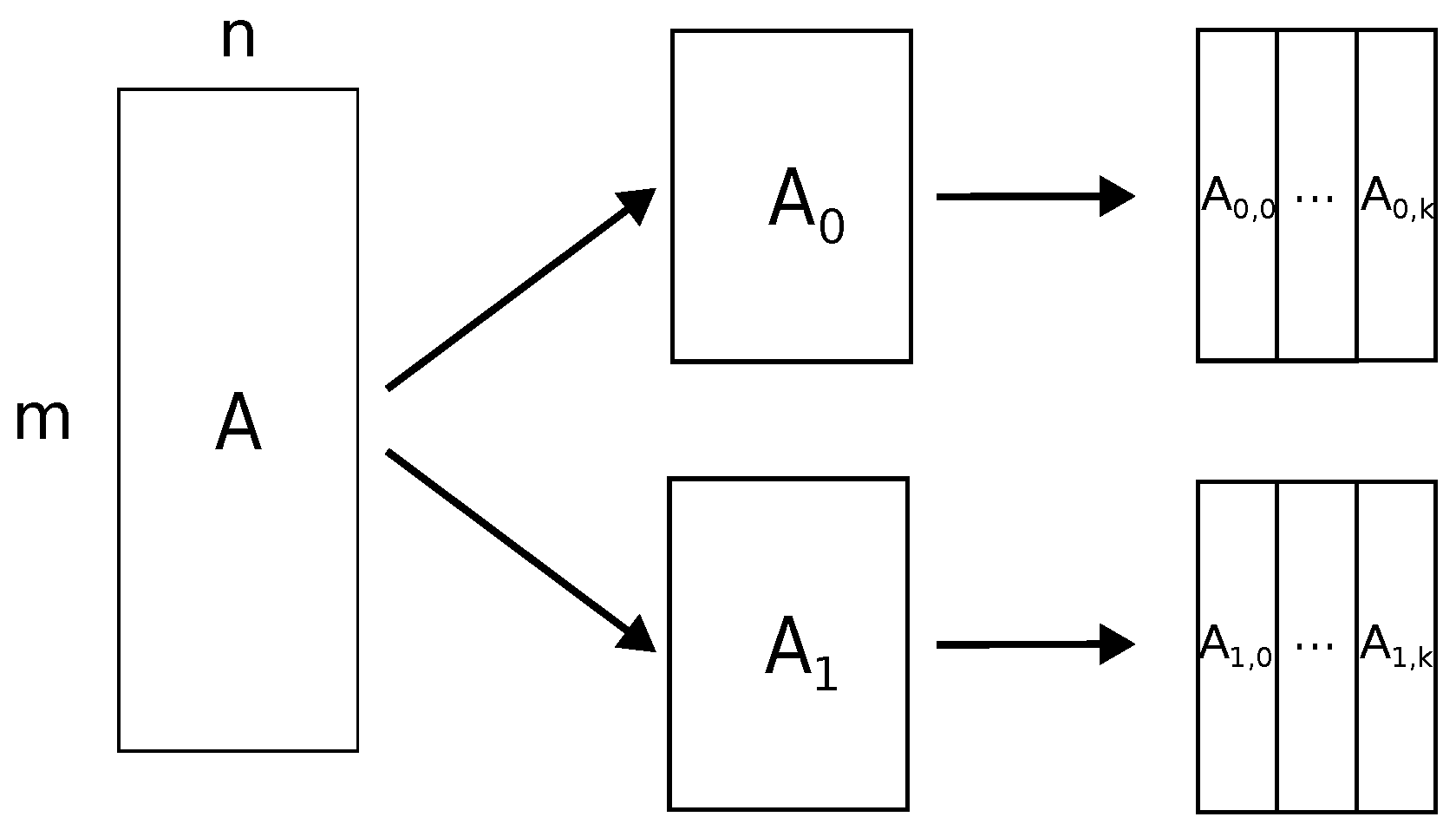
Analysing Algorithm 1, one can observe that the computationally most expensive steps (in lines 2, 4, 6 and 7) are performed on panels with full row rank, utilising level-3 BLAS kernels (matrix multiplications). Since the arithmetic intensity (i.e., the ratio between floating point operations and total data movement) of the level-3 BLAS kernels is $\mathcal{O}\left(m\right)$, where m is the dimension of a matrix, the required communication can be efficiently overlapped with effective computation (compute-bound operations). Therefore, we proposed a distributed version in which the input matrix A is partitioned and distributed among P processors in a one-dimensional block row layout (see Figure 2 middle). Each block row $A_p$ is locally partitioned into k panels $A_{p,j}$ with width $b=n/k$ columns and $j\in \{1,\dots ,k\}$. The proposed block row partitioning allows for coarse-grained parallelisation between processes (inter-node level), while partitioning into panels exploits fine-grained parallelisation at the node level.

Figure 2. Distributing and slicing of a matrix. An example with 2 processors. The assignments of blocks and panels with processors are indicated on the vertical axis.

The distributed CholeskyQR algorithm with blocked Gram–Schmidt is described in Algorithm 2. The algorithm processes the input matrix A by panels, starting from the leftmost one. The first step is to calculate the Gram matrix. Each processor computes a local Gram matrix from its current panel $A_{p,j}$ (line 2) and sums over all local matrices to obtain the final Gram matrix (line 3). Summing and distributing require collective communication (using e.g., MPI_Allreduce), after which all processors have an identical Gram matrix. The Cholesky factorisation (line 4) is computed redundantly on each processor, and to avoid additional communication overhead, each processor updates only its block row $Q_{p,j}$ of the orthogonal panel $Q_j$ (line 5). Updating the panels to the right of the current panel requires communication between processors, since the panel $Q_j$ is applied to the full row rank of the trailing matrix $A_{p,j+1:k}$ (lines 7–9). Each processor first calculates its partial product $Y_p$ (line 7), and then a collective communication (line 8) is required to sum and broadcast the global Y. Once the intermediate matrix Y has been transmitted, each block row can be updated independently (line 9).

Algorithm 2 Distributed Cholesky QR with blocked Gram–Schmidt
Input: Number of processors P, $A\in {\mathbb{R}}^{m\times n}$ partitioned into block rows and distributed among processors, panel width b
Output: $Q\in {\mathbb{R}}^{m\times n}$ orthogonal and $R\in {\mathbb{R}}^{n\times n}$ upper triangular matrix
1: for j = 1, 2, …, k do
2:       $W_{p,j}:=A_{p,j}^T{A}_{p,j}$
3:       $W_j:=\mathrm{MPI}\_\mathrm{Allreduce}\left(W_{p,j}\right)$	▹ Communication
4:       $W_j=U^{T}U$
5:       $Q_{p,j}:=A_{p,j}{U}^{-1}$
6:       $R_{j,j}:=U$
7:       $Y_p:=Q_{p,j}^T[A_{p,j+1},A_{p,j+2},\dots ,A_{p,k}]$
8:       $Y:=\mathrm{MPI}\_\mathrm{Allreduce}\left(Y_p\right)$	▹ Communication
9:       $[A_{p,j+1},\dots ,A_{p,k}]:=[A_{p,j+1},\dots ,A_{p,k}]-Q_{p,j}Y$
10:     $[R_{j,j+1},R_{j,j+2},\dots ,R_{j,k}]:=Y$
11: end for

A special case occurs when the width of the panel b is set equal to the number of columns n. This configuration eliminates the iteration over j and the panel updates, effectively removing the Gram–Schmidt component. In this case, CQRGS2 reverts to the standard CholeskyQR2 algorithm, resulting in equivalent computational and communication costs.

A detailed breakdown of the computational and communication complexity for each subroutine can be found in Table 1. The total complexity cost of the parallel CholeskyQR2 with Gram–Schmidt (CQRGS2) is dominated by the expression $4{\displaystyle \frac{m{n}^2}{P}}$ that arises from the total cost of the routines SYRK, TRSM, and UPDATE, which correspond to the construction of the Gram matrix, computation of the orthogonal matrix, and updating part of the Gram–Schmidt process, respectively. As these do not depend on the panel width b, the computational complexity of these parts can be reduced by using more processors and thus exploiting more parallelism. In contrast, the first and last terms in the total computational cost of CQRGS2, which correspond to the Cholesky factorisation and the matrix addition performed in the reduction calls, do depend on the panel width b. Therefore, b can be considered an optimisation parameter that can be adjusted to achieve either improved numerical accuracy (see Figure 3), such as increased matrix orthogonality, or faster computation. This approach, characterised by the parameter b, not only increases numerical stability but also reduces the overall computational complexity compared to the conventional CholeskyQR2 algorithm.

Table 1. Computational (up) and communication (down) complexity of CholeskyQR2 with Gram–Schmidt (GS).

Algorithm		Routine	Total Comp
CQRGS2	CQRGS	Gram	$bn{\displaystyle \frac{m}{P}}$
		Gram_reduce	$bnlo{g}_{2}P$
		Cholesky	${\displaystyle \frac{b^{2}n}{3}}$
		Construct_Q	${\displaystyle \frac{bmn}{P}}$
		GS	$2{\displaystyle \frac{mn}{P}}(n-b)$
		GS_reduce	${\displaystyle \frac{n}{2}}(n-b)lo{g}_{2}P$
		Total	${\displaystyle \frac{b^{2}n}{3}}+2{\displaystyle \frac{m{n}^2}{P}}+{\displaystyle \frac{n}{2}}(n+b)lo{g}_{2}P$
	Compute_R		${\displaystyle \frac{n^3}{3}}$
	Total		$2{\displaystyle \frac{b^{2}n}{3}}+{\displaystyle \frac{n^3}{3}}+4{\displaystyle \frac{m{n}^2}{P}}+n(n+b)lo{g}_{2}P$
			Total Comm	# of Calls
CQRGS2	CQRGS	Gram_reduce	$bnlo{g}_{2}P$	${\displaystyle \frac{n}{b}}$
		GS_reduce	${\displaystyle \frac{1}{2}}n(n-b)lo{g}_{2}P$	${\displaystyle \frac{n}{b}}-1$
	Total		$n(n+b)lo{g}_{2}P$	${\displaystyle \frac{4n}{b}}-2$

Figure 3. CQRGS2: Orthogonality of Q as a function of panel size, for ill-condition input matrices with m = 30,000, n = 3000.

4.1. Analysis of Numerical Stability

The reason numerical stability depends on the value of b is that, when the input matrix A is divided into panels, the condition number of the first panel can be significantly reduced. The dependence of numerical stability on the panel width b was formally established by the authors of [15] in their stability analysis of block Gram–Schmidt methods. Since the condition number is the ratio of the largest to the smallest singular value, the upper and lower bounds of the singular values of the submatrix (i.e., panel) $B\in {\mathbb{R}}^{m\times r}$ of the original matrix $A\in {\mathbb{R}}^{m\times n}$ with $n-r$ columns removed and $r<n$ are required.

Let ${\sigma }_1\ge {\sigma }_2\ge \dots \ge {\sigma }_{n-1}\ge {\sigma }_n$ be the singular values of A, and ${\gamma }_1\ge {\gamma }_2\ge \dots \ge {\gamma }_{r-1}\ge {\gamma }_r$ singular values of B. Then the following inequalities hold:

$${\sigma }_i\ge {\gamma }_i,i=1,2,\dots ,r$$

(2)

$${\gamma }_i\ge {\sigma }_{i+(n-r)},i\le r.$$

(3)

For a proof, see Corollary 8.6.3 in [4]. From the above inequalities, the largest and smallest singular values of B are bounded by

$${\sigma }_1\ge {\gamma }_1\ge {\sigma }_{1+(n-r)}$$

(4)

$${\sigma }_r\ge {\gamma }_r\ge {\sigma }_n$$

(5)

The condition number of B is then

$$cond\left(A\right)={\displaystyle \frac{{\sigma }_1}{{\sigma }_n}}\ge cond\left(B\right)\ge {\displaystyle \frac{{\sigma }_{1+(n-r)}}{{\sigma }_r}}.$$

(6)

In the general case, where the singular values of the original matrix A are evenly distributed, the condition number of a panel B is significantly smaller than the upper bound. This property underpins our strategy: the panel width b is chosen so that the condition number of the first panel, $\kappa \left(A_1\right)$, is sufficiently small. The objective is to ensure that its corresponding Gram matrix, $A_1^T{A}_1$, is positive definite. Since the condition number of the Gram matrix is $\kappa {\left(A_1\right)}^2$, we can select b so that this value remains below the computational limit of $\mathcal{O}\left({ϵ}^{-1}\right)$ (approximately ${10}^{15}$ in double precision arithmetic).

This strategy fails in the worst-case scenario, which occurs when the singular values are clustered around an extremely large value. In such cases, the condition number of the panel equals that of the original matrix, rendering the CQRGS2 algorithm unstable. While we acknowledge this limitation, such extreme cases are not the focus of this research and are left for future work.

The choice of panel width b directly controls the trade-off between numerical stability and computational performance. For example, with panel size $b=1500$ and condition number $\kappa \left(A\right)={10}^{13}$, the stability is maintained, but the loss of orthogonality increases significantly (see Figure 3). For highly ill-conditioned matrices, such as $\kappa \left(A\right)={10}^{15}$, maintaining numerical stability requires a small panel width (e.g., $b=300$). This strategy effectively partitions the matrix into a larger number of better-conditioned subproblems, ensuring the final loss of orthogonality remains at the desired order of $\mathcal{O}\left(ϵ\right)$. However, this improved stability comes at a significant performance cost. A small b increases the number of panels (in this case, to 10), which in turn increases the number of iterations over the main loop in Algorithm 2 (lines 2–10). Each iteration contains two collective communication steps (lines 3 and 8), making these synchronisation points a major performance bottleneck.

For well-conditioned matrices, a larger panel width can be used to reduce the number of iterations and improve performance. For example, with $\kappa \left(A\right)={10}^{13}$ and panel size $b=1500$, the algorithm is computationally stable, but this choice leads to a significant degradation in orthogonality, as illustrated in Figure 3. This trade-off is eliminated for well-conditioned matrices (e.g., $\kappa \left(A\right)<{10}^8$), where, as shown in Figure 1, additional Gram–Schmidt reorthogonalisation steps are not required. In such cases, the algorithm can be configured with $b=n$, which effectively reduces it to the standard CholeskyQR method.

4.2. Performance Analysis

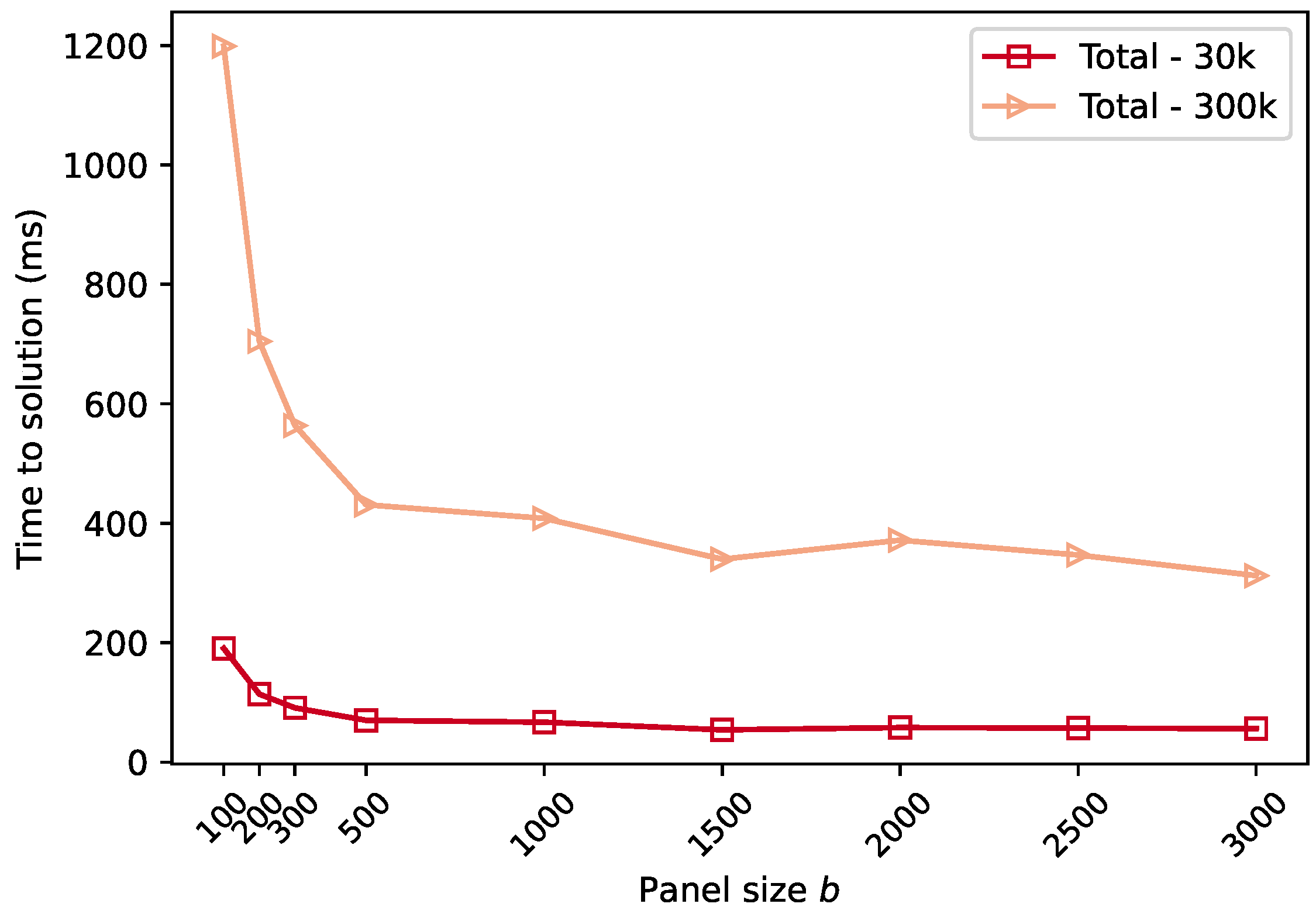
The choice of panel width introduces a performance trade-off between communication volume and communication frequency. Its effect on total execution time is shown in Figure 4, which clearly demonstrates that increasing panel width b decreases the execution time. However, as detailed in Table 1, a smaller b reduces the size of the Gram matrix constructed in each step (Algorithm 2, lines 2–3). This results in a substantial reduction in the total volume of data that must be communicated, as shown by comparing the total communication cost of the distributed CQRGS2,

$$n(n+b){log}_{2}P,$$

(7)

to the $2n^2{log}_{2}P$ cost of CholeskyQR2. The time savings from reducing and broadcasting a smaller Gram matrix more than compensate for the additional communication introduced by the Gram–Schmidt process (Algorithm 2, line 8), provided that $b\ll n$.

Figure 4. Time to solution of CQRGS2 on 4 GPUs as a function of panel size for well-conditioned input matrices ($\kappa \left(A\right)={10}^4$) with $m=\mathrm{30,000}$ and $\mathrm{300,000}$ and a fixed number of columns $n=3000$.

However, the main drawback of a small panel width is the increase in communication frequency. A smaller b results in a larger number of panels, which increases the number of collective communication calls required. The number of messages scales with ${\displaystyle \frac{4n}{b}}$; consequently, halving the panel width doubles the number of required synchronisation events. In modern distributed systems, latency costs from frequent synchronisations often dominate total execution time, outweighing the benefits of reduced flop counts and lower data volume. This effect is clearly illustrated in Figure 4: although using a smaller panel width (e.g., $b=100$) reduces the total flops, the execution time is significantly longer than when using fewer, larger panels (e.g., $b=1500$) due to the high latency overhead.

This analysis highlights the central dilemma of this approach. According to Figure 3, achieving numerical stability for matrices with condition number $\mathcal{O}\left({10}^{15}\right)$ requires a smaller panel width that creates 10 panels. Yet, as shown by the performance data, this configuration is far from optimal. The algorithm is therefore caught in a state where the parameters required for numerical robustness are detrimental to performance. This motivates the need for a modified approach that can achieve stability without relying on a prohibitively large number of panels.

5. Mixed Block Gram–Schmidt with CholeskyQR

The analysis in the previous section established a fundamental trade-off in the CQRGS2 algorithm: the large number of panels required to ensure numerical stability for ill-conditioned matrices leads to a prohibitive number of synchronisation points, which severely degrades performance. To overcome this limitation, we introduce a novel algorithm that reorders the orthogonalisation steps to achieve stability without requiring an excessive number of panels. The core of the new method is a more robust, two-pass local process for orthogonalising each panel. This approach allows the use of larger (and thus fewer) panels, directly addressing the performance bottleneck. For a given number of panels, the computational complexity and communication costs of this new algorithm are equivalent to those of CQRGS2 (Table 2); its advantage lies in its ability to achieve numerical stability with fewer panels. This provides a panelling strategy that is effective for both ill- and well-conditioned matrices and does not require additional operations for ill-conditioned matrices compared to well-conditioned.

Table 2. Summary of complexities, stability and condition for stability for parallel CholeskyQR-based algorithms and TSQR for an $m\times n$ matrix executed in parallel with P processes.

Algorithm	Complexity		Stability	Condition
	Computation	Communication
CQR2	$4m{n}^2/P$	$n^2{log}_{2}P$	$\mathcal{O}\left(ϵ\right)$	$\mathcal{O}\left(ϵ\right){\kappa }^2\left(A\right)<1$
CQRGS2	$4m{n}^2/P$	$n(n+b){log}_{2}P$	$\mathcal{O}\left(ϵ\right)$	$\mathcal{O}\left(ϵ\right){\kappa }^2\left(A_j\right)<1$
sCQR3	$6m{n}^2/P$	${\displaystyle \frac{3}{2}}{n}^2{log}_{2}P$	$\mathcal{O}\left(ϵ\right)$	$\mathcal{O}\left(ϵ\right)\kappa \left(A\right)<1$
mCQRGSI+	$4m{n}^2/P$	$n(n+b){log}_{2}P$	$\mathcal{O}\left(ϵ\right)$	$\mathcal{O}\left(ϵ\right){\kappa }^2\left(A_j\right)<1$
TSQR	$4m{n}^2/P$	$n^2{log}_{2}P$	$\mathcal{O}\left(ϵ\right)$	none

Algorithm 3 presents the proposed mixed block Gram–Schmidt algorithm (mCQRGSI+), expressed in a format consistent with Algorithms 1 and 2 and omitting distributed parallelisation specifics for clarity. Unlike CQRGS2, which improves stability by looping twice over all panels, the proposed method performs a single traversal but applies a strengthened two-pass orthogonalisation to each panel. The first panel is orthogonalised using CQR2 (line 1), forming the initial orthonormal block $Q_1$. The computation then proceeds sequentially over panels $A_j$, $j\ge 2$. $A_j$ and all panels to its right are reorthogonalised (lines 3–4) against the most recently completed block $Q_{j-1}$ using a modified Gram–Schmidt update to eliminate components already represented in the basis. Then a single CQR pass is applied on updated $A_j$ (line 6), following the panel reorthogonalisation with respect to all previously computed panels $\{Q_1,\dots ,Q_{j-1}\}$ (lines 7–8) to restore global orthogonality. The final CQR step (line 9) ensures internal orthogonality of the updated panel and consistency with the global basis. This process guarantees the complete orthogonalisation of panel $A_j$ and its orthogonality to the previously orthogonalised panels.

Algorithm 3 Mixed Block Gram–Schmidt with CholeskyQR (mCQRGSI+)
Input: $A\in {\mathbb{R}}^{m\times n}$, number of panels k
Output: $Q\in {\mathbb{R}}^{m\times n}$ orthogonal and $R\in {\mathbb{R}}^{n\times n}$ upper triangular matrix
1: $Q_1,R_{1,1}=CQR2\left(A_{:,1}\right)$	▹ Orthogonalize first panel
2: for $j=2\dots k$ do
3:       $Y:=Q_{j-1}^T{A}_{:,j:k}$	▹ Projections of orthogonal panels on non-orthogonal
4:       ${\widehat{A}}_{:,j:k}:=A_{:,j:k}-Q_{j-1}Y$	▹ Update panels $A_j,\dots A_k$
5:       $[R_{j-1,j},R_{j-1,j+1},\dots ,R_{j-1,k}]:=Y$
6:       $Q_{tmp},R_{tmp}=CQR\left({\widehat{A}}_{:,j}\right)$
7:       $Y:=Q_{1:j-1}^T{Q}_{tmp}$
8:       ${\widehat{Q}}_{tmp}:=Q_{tmp}-Q_{1:j-1}Y$	▹ Reorthogonalise current panel
9:       $Q_j,R_{j,j}=CQR\left({\widehat{Q}}_{tmp}\right)$
10:      $R_{1:j-1,j}:=R_{1:j-1,j}+Y\ast R_{tmp}$
11:      $R_{j,j}:=R_{j,j}\ast R_{tmp}$	▹ Construct final R
12: end for

The parallelisation strategy is similar to that presented in Algorithm 2, distributing the matrix A into row-blocks as depicted in Figure 2. The algorithm requires one synchronisation point in each of the inner orthogonalisation routines (CQR, lines 6 and 9) for constructing the Gram matrix. Another two synchronisation points, one for each reorthogonalisation step, are required when constructing the temporary product Y (lines 3 and 7). An example of how the matrix divided into three panels is processed by 4 MPI ranks is shown in Figure 5.

Figure 5. Schematic representation of the matrix distribution across 4 processes and the associated operations performed on local matrix data. Computations on the panels are highlighted in red, final results in green and partially updated panels in orange.

The new algorithm is denoted by mCQRGSI+, following the naming convention proposed in [16]. The suffix “I+” stands for repeated inner reorthogonalisations, compared to the suffix “2” which indicates that the algorithm is repeated twice, such as CholeskyQR2 (CQR2).

Numerical Stability Analysis

The stability and performance of the mCQRGSI+ algorithm stem from its hybrid use of both modified and classical Gram–Schmidt methods. This design is motivated by the varying numerical properties of the data at different stages of the algorithm.

The first reorthogonalisation step (lines 3–4) is the most numerically sensitive, as it operates on the trailing submatrix, which may contain ill-conditioned panels. For this reason, the robust Block Modified Gram–Schmidt (BMGS) is applied to ensure stability during this critical phase. Subsequently, an initial pass of CQR is applied to the current panel (line 6). While this does not guarantee full orthogonality of the computed matrix $Q_j$, it significantly improves its condition number, making it nearly orthogonal ($\kappa \approx 1$).

Because the panel is now well-conditioned, the second reorthogonalisation step (lines 7–8) can safely employ the more efficient Block Classical Gram–Schmidt (BCGS) to orthogonalise against the panels to the left. The key advantage of BCGS in this context is that it can be performed in a single computational step, requiring only one collective communication (Allreduce) per panel, which is a significant performance optimisation.

The overall stability of this hybrid approach can be understood through the framework established in the literature and by analysing the stability of Block Gram–Schmidt (BGS) algorithms. The authors in [16] decomposed a BGS algorithm into its high-level structure (the skeleton) and its inner panel factorisation (the muscle) and established the dependency of the final stability of the algorithm on the stability of the skeleton. The high-level structure of our algorithm (i.e. the skeleton) is a combination of BMGS and BCGS and is similar to Algorithm 4 (BCGSI+) in [16,28], albeit with some key distinctions. Given that BMGS is inherently more stable than BCGS [28,29], the stability of mCQRGSI+ is at least as good as that of the pure BCGSI+ skeleton, which was demonstrated in [29] to achieve an $\mathcal{O}\left(ϵ\right)$ loss of orthogonality provided that $\mathcal{O}\left(ϵ\right)\kappa \left(A\right)<1$.

However, the stability of the skeleton depends on the stability of the inner orthogonalisation routine, which in our case is the CholeskyQR algorithm. Following the numerical analysis in [28,30], the loss of orthogonality of mCQRGSI+ is bounded by

$$\left|\right|I-Q^{T}Q{\left|\right|}_2<\mathcal{O}\left(ϵ\right)$$

(8)

under the condition that for each panel $A_j$

$$\mathcal{O}\left(ϵ\right){\kappa }^2\left(A_j\right)<1.$$

(9)

In other words, this condition requires that the condition number of each panel is small enough (<10⁸ in double precision arithmetic) to ensure the numerical stability of the inner CholeskyQR (CQR) routine. When this assumption holds, the inner orthogonalisation is stable, and our algorithm, like BCGSI+ from [30], achieves a final loss of orthogonality close to machine precision.

A comparison of the execution cost and numerical stability of mCQRGSI+ with other algorithms is provided in Table 2. Note that CQRGS2 and mCQRGSI+ exhibit the same complexity and comparable stability under similar conditions. However, CQRGS2 requires an increased number of panels to control the loss of orthogonality for very ill-conditioned matrices (see Figure 3 for $\kappa \left(A\right)>{10}^{10}$), whereas mCQRGSI+ maintains stable performance without increasing the panel count. TSQR is a Householder-based algorithm that achieves the machine-precision stability (i.e., minimal loss of orthogonality) regardless of condition number and thus serves as a baseline for evaluating numerical stability.

6. Scalability Analysis

In this section, the strong and weak scaling performance of the Modified CholeskyQR2 with Gram–Schmidt (mCQRGSI+) is analysed and compared with the ScaLAPACK and SLATE counterparts. In our benchmarks, the 3-panel strategy in mCQRGSI+ is used for all test cases, as it has been shown to achieve the required numerical stability $\mathcal{O}\left(ϵ\right)$ even for extremely ill-conditioned matrices. For the GPU version, the NCCL library was used for collective communication instead of CUDA-aware MPI, as NCCL achieves much better performance by significantly reducing communication overhead.

6.1. Strong Scalability

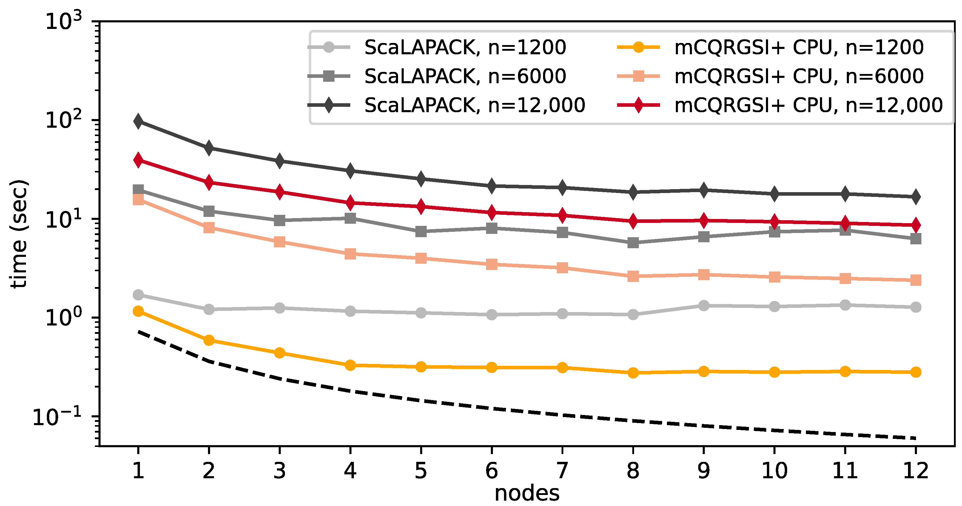
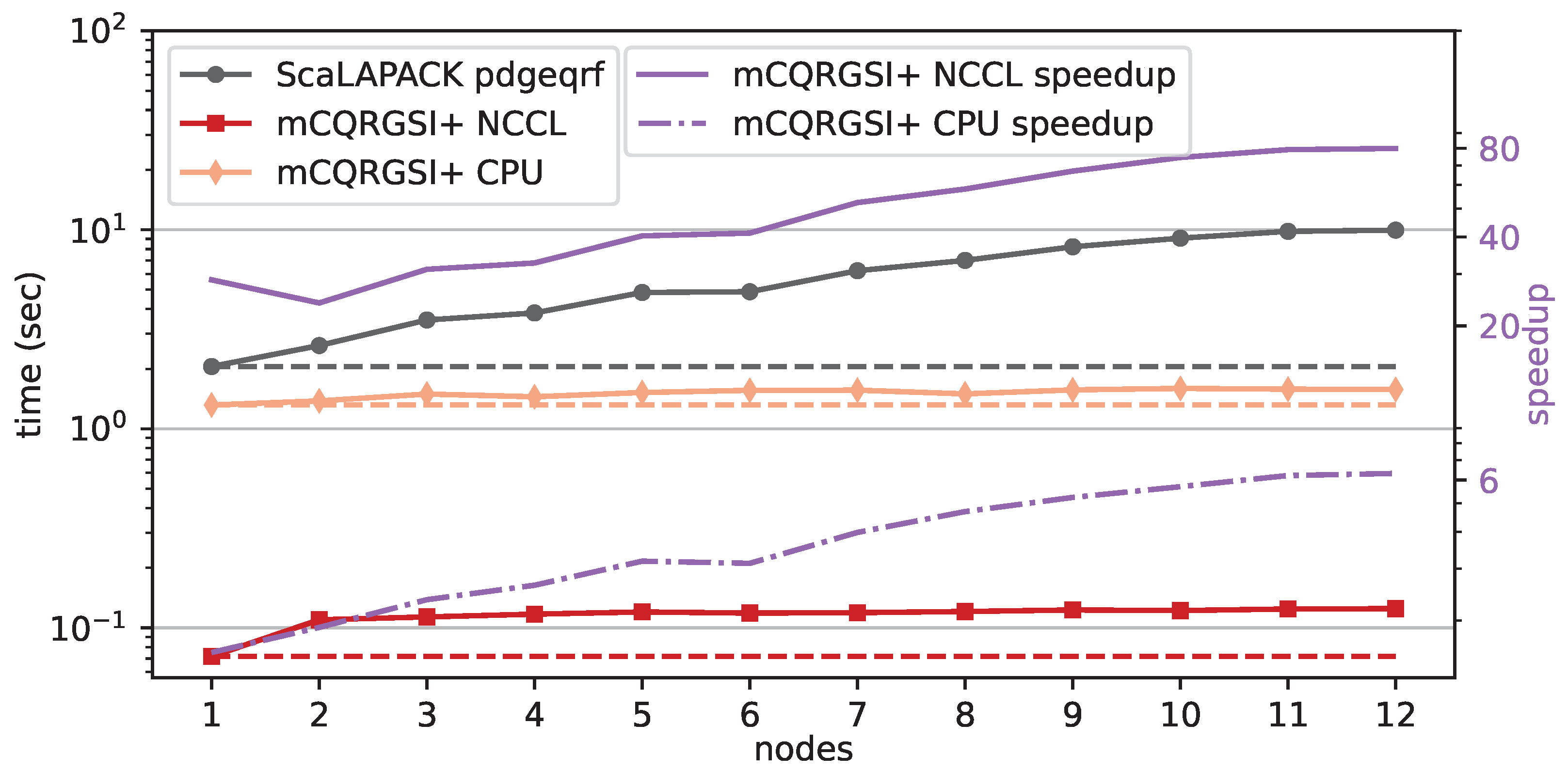
Strong scalability was tested on the three artificial matrices (see Section 3) with condition number $\kappa \left(A\right)={10}^4$ and dimensions 120k × 1.2k, 120k × 6k and 120k × 12k (the panel sizes are $400,2000$, and 4000, respectively). Figure 6 illustrates the strong scaling behaviour of the CPU-only version of mCQRGSI+ and ScaLAPACK PDGEQRF. The mCQRGSI+ CPU outperforms ScaLAPACK by up to $4.7\times$ ($9.4\times$ for PDORGQR + PDGEQRF) on all test matrices. Figure 7 shows the corresponding results for the GPU version based on NCCL and SLATE CQR2.

Figure 6. Strong scaling of mCQRGSI+ and ScaLAPACK’s pdgeqrf with artificial matrices $m=120\mathrm{k}$, $n=\{1.2\mathrm{k},6\mathrm{k},12\mathrm{k}\}$ w.r.t. the number of nodes. The dashed line is the ideal scaling.

Figure 7. Strong scaling of mCQRGSI+ NCCL with artificial matrices $m=120\mathrm{k}$, $n=\{1.2\mathrm{k},6\mathrm{k},12\mathrm{k}\}$ w.r.t the number of nodes. The dashed line is the ideal scaling.

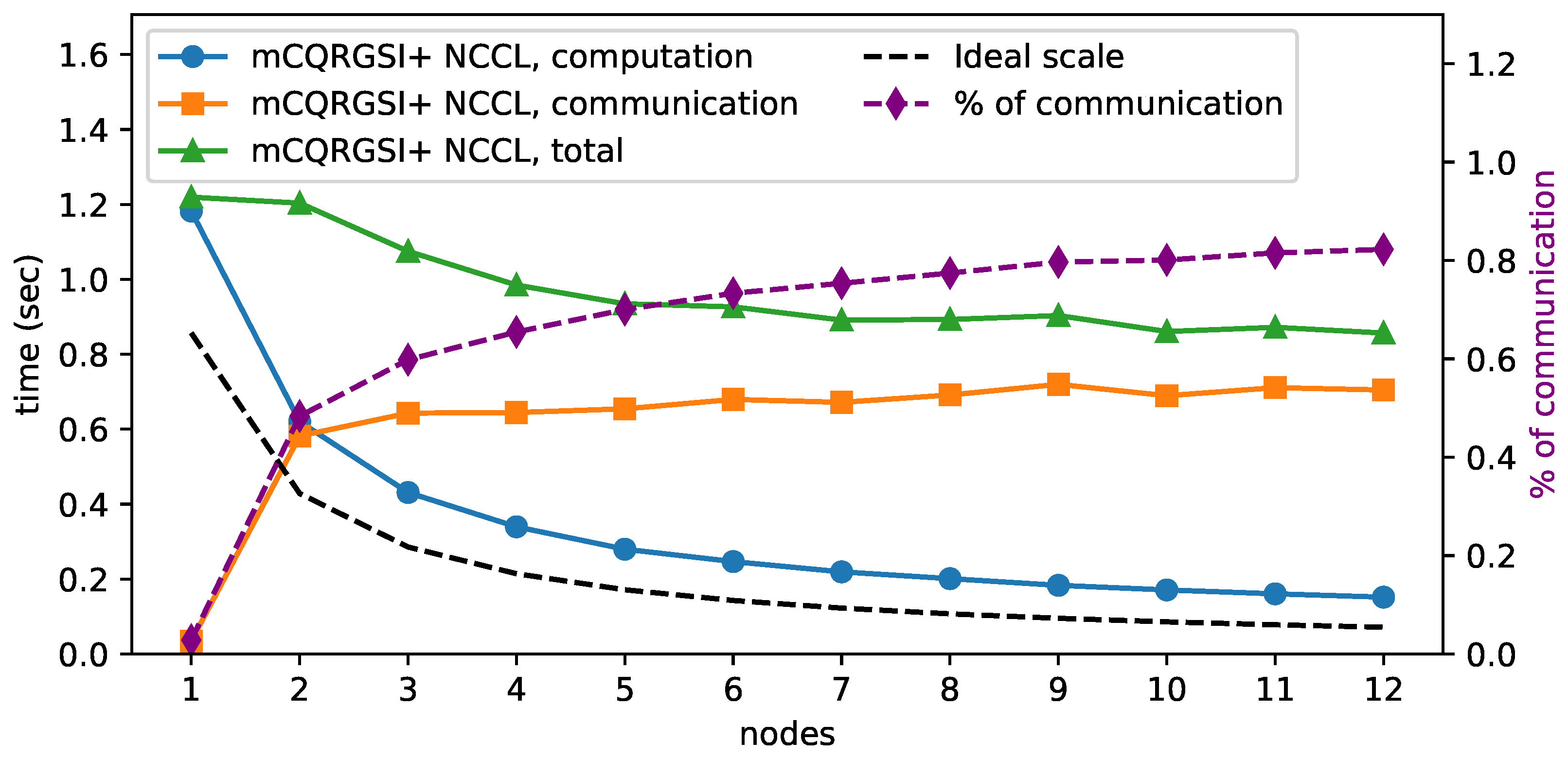
The scalability of mCQRGSI+, however, decreases with the number of nodes. This is due to the Allreduce operation required in constructing the Gram matrix performed in CQR calls (Algorithm 3, lines 6 and 9), which does not scale with the number of nodes. In strong scaling tests, the width of the panel is fixed, resulting in a constant load in Gram reduction operations, while the communication load increases with the number of nodes, as shown in Figure 8 (orange line). Although the computation scales close to the ideal line, the communication time slightly increases with the number of nodes, resulting in lower overall scalability. In our test cases, starting from 3 nodes, communication becomes dominant and reaches up to $80\%$ of the total execution time (purple line) on 12 nodes. This also explains the stagnation of speedup from 3 nodes onwards, when communication starts to dominate, which also occurs for matrices with 6000 and 12,000 columns. For larger matrices with $m=300$k, communication becomes dominant on 12 nodes and accounts for ≈55% of total execution time.

Figure 8. Total execution time (green), computation (blue) and communication (yellow) of mCQRGSI+ on GPU. The percentage of the communication in the total execution time is given in purple. Matrix size is $120\mathrm{k}\times 12\mathrm{k}$.

Figure 9 shows the speedup of mCQRGSI+ MPI for a varying number of columns over the SLATE CQR2 implementation. Both algorithms use MPI for communication and exploit all available GPUs. The execution time of mCQRGSI+ is, for nearly all numbers of nodes, lower than that of SLATE CQR2. However, since the SLATE implementation was not specifically designed for tall-and-skinny matrices, the performance difference decreases with an increased number of columns (e.g., $30\mathrm{k}$). The lack of scaling observed in these results can be attributed to the communication performance described above, which is further exacerbated when distributed GPU nodes are used.

Figure 9. mCQRGSI+ speedup over SLATE CQR2 on GPUs for matrix sizes $m=300\mathrm{k}$, $n=\{3\mathrm{k},15\mathrm{k},30\mathrm{k}\}$. mCQRGSI+ is using the 3-panel strategy.

6.2. Weak Scalability

Weak scaling experiments demonstrate the potential of the novel algorithm to perform computations on large matrices while maintaining a constant load per process or node. The tests were conducted for the CPU-only version and both GPU versions (using MPI and NCCL communicators) of mCQRGSI+. The first analysis compared our algorithm with the ScaLAPACK implementation. The ScaLAPACK configuration used 16 tasks (MPI processes) per node and 8 threads per task, with the block height set to the number of rows divided by the number of MPI processes and the block width set to 32. This configuration achieved the best performance in our “sweet spot” analysis.

Figure 10 shows that the weak scaling is nearly optimal for both the CPU and GPU versions of mCQRGSI+, with the total execution time ranging from $71.78$ ms on one node to 124 ms on 12 nodes for the GPU version. A steep increase in time from one to two nodes ($1.53\times$) is due to the NCCL communication overhead, which was not observed when all NCCL processes were on the same node. Although the introduction of inter-node communication is significant when switching to two nodes, it remains almost constant as more nodes are added. Note that the performance of ScaLAPACK decreases as the number of nodes increases. Since the number of columns is fixed, the matrices become increasingly thin as the number of nodes increases (i.e., a fixed number of rows per process/node), resulting in significant performance degradation for ScaLAPACK, which is optimised for general and square matrices rather than tall-and-skinny matrices. Although communication in mCQRGSI+ is significant compared to the total execution time (see Figure 8), both the GPU and CPU versions of the code achieve substantial speedup compared to ScaLAPACK, with the CPU variant achieving a $6\times$ speedup and the GPU variant with the NCCL communicator an $80\times$ speedup. However, if both ScaLAPACK’s routines PDORGQR and PDGEQRF are considered (for details, see Section 2), the speedup gains double to $12\times$ and $160\times$, respectively. Figure 10 also demonstrates that the superior performance of our algorithm does not result from the use of GPUs but from the careful design of the algorithm tailored to the special matrix shape and condition.

Figure 10. Weak scaling of mCQRGSI+ CPU, mCQRGSI+ and SCALAPACK (pdgeqrf only) with block row $40\mathrm{k}\times 3\mathrm{k}$. Dashed lines are the ideal scaling.

Similarly, before the scaling analysis, a parametric study of the SLATE runtime options was performed to identify the optimal runtime configuration. The combination with OMP_NUM_THREADS=8, square SLATE tile sizes of $min(n,4096)$ where n is the number of columns of the matrix, Lookahead = 2, and a linear arrangement of MPI processes (SLATE parameters p, q), where p is the number of nodes and q = 1, was identified as optimal for our case. The optimal tile size of 4096 double-precision floating-point numbers allows 320 tiles to fit in the 40 GB memory of a single A100 GPU and 32 tiles in its L2 cache. All SLATE jobs were run with a single MPI process per node, eight OpenMP threads, and the maximum four GPUs per node. The Cray Parallel Application Launch Service (PALS) was invoked with the ‘–ppn 1 -d 8 –cpu-bind depth’ flags.

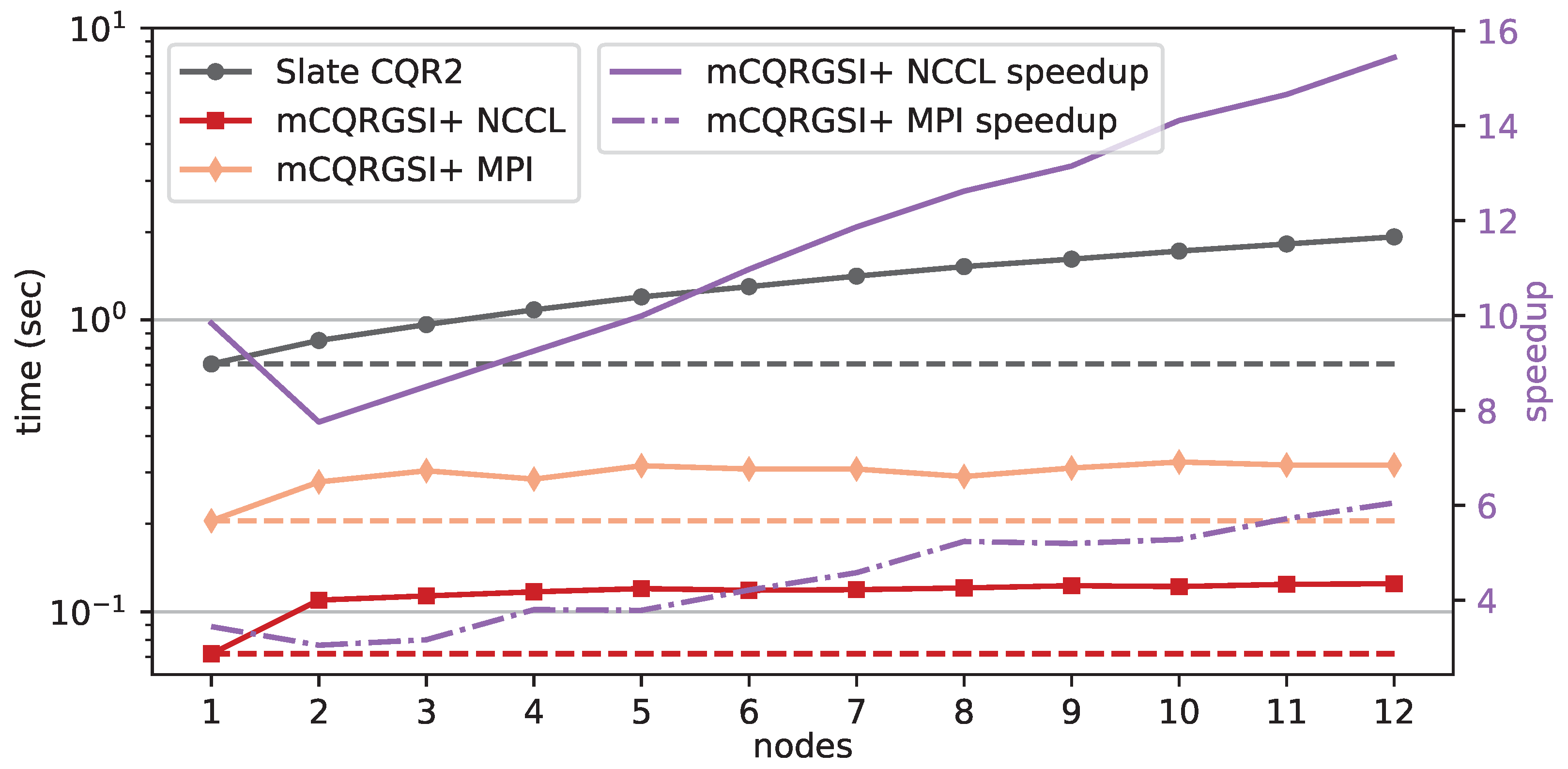
The results in Figure 11 show that the implementation of CQR2 in SLATE is $3.75$ to 6 times slower than mCQRGSI+ using MPI. Given that communication overhead dominates the algorithm execution time when MPI is used, especially as the number of nodes increases (as shown in Figure 8), the observed difference mainly arises from the different communication routines used by the two implementations. SLATE is a general-purpose linear algebra library that supports arbitrary-sized tile handling, including sending and receiving tile data across distributed computers via a custom implementation of a hypercube broadcast pattern using MPI send and receive routines (MPI_Irecv and MPI_Isend). The total communication volume in the SLATE Cholesky QR implementation (called twice in CQR2) depends on the tile size, the n_lookahead parameter, and the number of OMP threads. In contrast, the mCQRGSI+ implementation simply uses Allreduce calls (Algorithm 2) that communicate matrices with dimensions equal to the panel width. Furthermore, the input matrix is statically scattered once, at the start of the algorithm, among all available GPUs to preserve data locality.

Figure 11. Weak scaling of mCQRGSI+ and Slate CholeskyQR2 with block row $40\mathrm{k}\times 3\mathrm{k}$. Dashed lines are the ideal scaling.

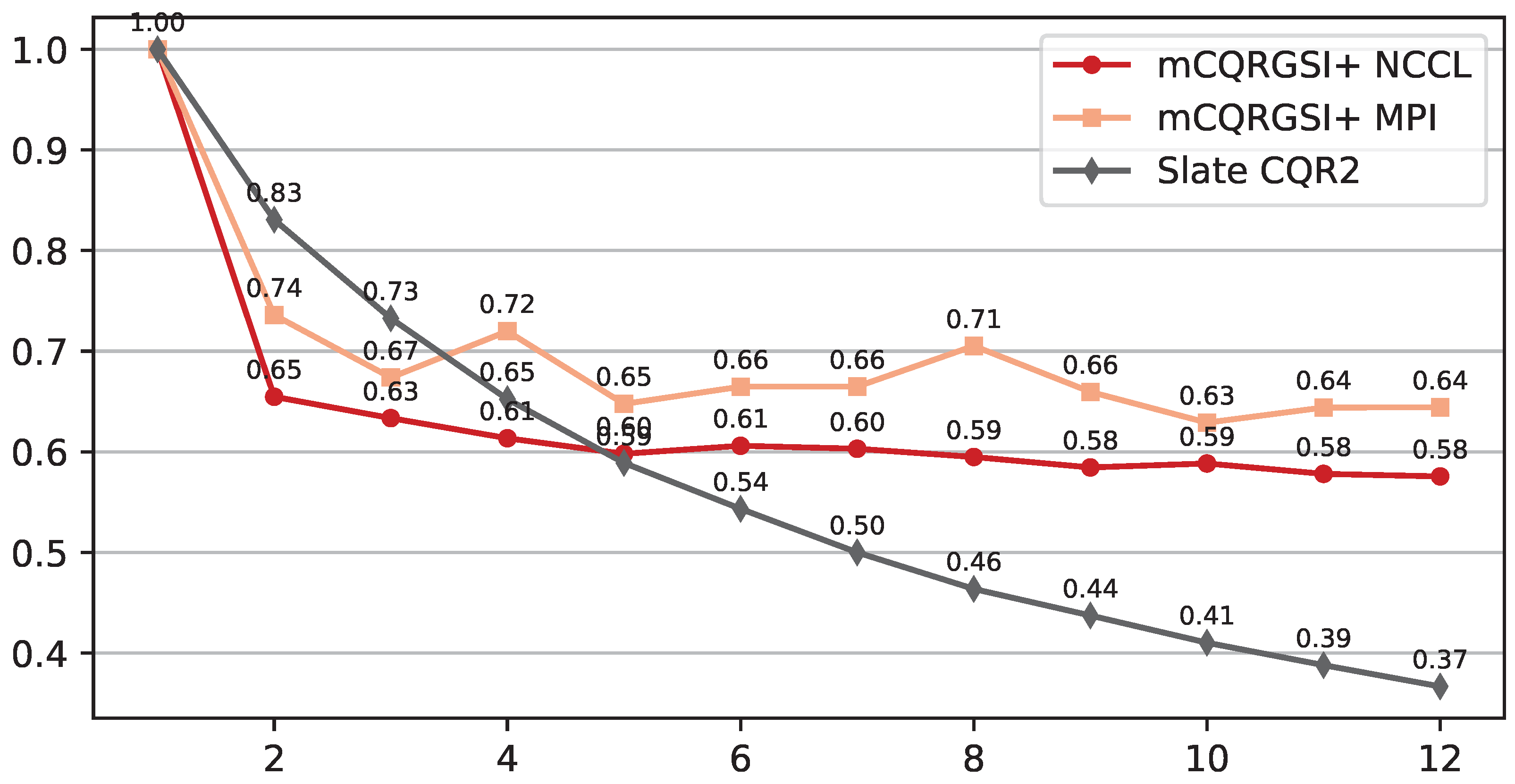
Figure 12 shows the parallel efficiency of the mCQRGSI+ variants and SLATE CQR2. Both the MPI and NCCL versions of mCQRGSI+ demonstrate good parallel efficiency as the problem size and node count increase, indicating that the algorithm’s performance scales predictably at larger scales. A notable feature is the significant initial overhead incurred when moving from one to two nodes, due to the introduction of inter-node communication. After this initial drop, the efficiency remains steady, consistent with the scalability trends shown in Figure 11. This indicates that despite its known communication overhead, our approach is well-suited for processing large-scale input matrices. In contrast, the SLATE CQR2 implementation is not well-suited for increasing problem sizes, as its communication overhead grows with system size, significantly limiting its scalability.

Figure 12. Parallel efficiency in weak scaling of mCQRGSI+ MPI, mCQRGSI+ NCCL and SLATE CQR2 with block row $40\mathrm{k}\times 3\mathrm{k}$.

A further characteristic is that the NCCL-based variant of mCQRGSI+ achieves lower weak scaling efficiency than its MPI-based counterpart, despite being consistently faster in absolute time. This behaviour is explained by their single-node performance: the mCQRGSI+ NCCL implementation has almost no communication overhead on a single node. Therefore, moving to two nodes introduces a large relative increase in communication cost, resulting in a steeper drop in efficiency than that observed for the MPI communicator, which has a non-zero communication overhead even on a single node.

7. Conclusions

This paper introduces mCQRGSI+, a novel Mixed Block Gram–Schmidt algorithm with CholeskyQR, designed to compute the QR factorisation of extremely ill-conditioned, tall-and-skinny matrices on distributed CPU and multi-GPU systems. The importance of mCQRGSI+ for the HPC and computational science communities lies in its demonstrated superior scalability and performance relative to state-of-the-art distributed QR factorisation algorithms, including those available in ScaLAPACK and SLATE. Its performance advantage arises from expressing all core computational steps as highly efficient level-3 BLAS operations, while simultaneously ensuring numerical robustness for very ill-conditioned tall-and-skinny matrices. Notably, mCQRGSI+ achieves stability without resorting to TSQR or other unconditionally stable Householder-based QR variants, which typically incur higher communication overheads and increased computational cost. The novelty of the algorithm lies in its strategy of ensuring complete orthogonalisation of the working panel before its use in the subsequent Gram–Schmidt step, thereby achieving greater numerical stability than methods such as CholeskyQR2.

The key findings demonstrate that mCQRGSI+ successfully maintains numerical stability close to machine precision for matrices with condition numbers as high as ${10}^{16}$. Furthermore, our algorithm proved to be significantly faster than established library implementations, outperforming the Householder-based QR factorisation from ScaLAPACK by a factor of 12 on distributed CPU systems and the CholeskyQR2 implementation from the SLATE library by up to 16× on GPU systems. This work presents a method that achieves both distributed parallelisability and numerical robustness.

However, the research also identified key limitations. The primary performance bottleneck is the collective communication required for Gram matrix construction, the cost of which scales with the number of compute nodes. Furthermore, the current panelling strategy, while effective for matrices with well-distributed singular values, is unable to ensure stability in cases involving highly clustered singular values.

Future work will proceed in two main directions. First, to address the performance bottleneck, we will investigate methods to reduce communication cost and explicitly overlap communication with computation. Second, to broaden the applicability of the algorithm, we will extend it with a shifting strategy to ensure numerical stability for matrices with challenging singular value distributions. Ultimately, mCQRGSI+ represents a significant advance in developing QR factorisation algorithms that achieve both numerical robustness and scalable performance on modern high-performance computing systems.

The source code of mCQRGSI+ is available on GitHub [31] and Zenodo [32]. Both repositories include instructions on how to compile and execute the code. Although we do not share the specific input matrix used for testing, the GitHub repository provides a simple matrix generator written in Python that constructs matrices with desired condition numbers and stores them in a format compatible with our experimental codes.