PINN Based on Domain Adaptation for Solving Fornberg–Whitham-Type Equations

Abstract

The Fornberg–Whitham equation, which contains high-order nonlinear derivatives, is widely recognized as a prominent model for describing shallow water dynamics. We explore physics-informed neural networks (PINsN) in conjunction with transfer learning technology to investigate numerical solutions for the FW equation. The proposed domain adaptation in transfer learning for PINN transforms the complex problem defined over the entire spatiotemporal domain into simpler problems defined over smaller subdomains. Training a neural network on these subdomains provides extra supervised learning data, effectively addressing optimization challenges associated with PINNs. Consequently, it enables the resolution of anisotropic and long-term predictive issues in these types of equations. Moreover, it enhances prediction accuracy and accelerates loss convergence by circumventing local optima in the specified scenarios. The method efficiently handles both forward and inverse FW equation problems, excelling in cost-effective accurate predictions for inverse problems. The efficiency and accuracy of our proposed approaches are demonstrated through examples and results.

1. Introduction

Partial differential equations (PDEs) play a critical role in modeling diverse physical phenomena in applied sciences and engineering. Solving the nonlinear PDEs linked with these phenomena is essential for a thorough understanding of certain problems in nature. It is noteworthy that many nonlinear PDEs demonstrate traveling wave solutions known as solitary wave solutions. An important instance is the Fornberg–Whitham equation, which depicts features of wave breaking behavior, fluid mechanical dynamics, and water propagation. The FW equation is stated in the form

$${\displaystyle \frac{\partial \varphi }{\partial t}}+{\displaystyle \frac{\partial \varphi }{\partial x}}-{\displaystyle \frac{\partial {\varphi }^3}{\partial x^2\partial t}}+\varphi {\displaystyle \frac{\partial \varphi }{\partial x}}=3{\displaystyle \frac{\partial \varphi }{\partial x}}{\displaystyle \frac{{\partial }^2\varphi }{\partial x^2}}+\varphi {\displaystyle \frac{{\partial }^3\varphi }{\partial x^3}},$$

(1)

which is proposed to model the behavior of wave breaking [1]. The variable $\varphi (x,t)$ is explicitly defined as the wave profile, with x and t representing the spatial and temporal coordinates. A generalized Fornberg–Whitham equation takes the form

$${\displaystyle \frac{\partial \varphi }{\partial t}}+{\displaystyle \frac{\partial \varphi }{\partial x}}-{\displaystyle \frac{\partial {\varphi }^3}{\partial x^2\partial t}}+\lambda \varphi {\displaystyle \frac{\partial \varphi }{\partial x}}=3{\displaystyle \frac{\partial \varphi }{\partial x}}{\displaystyle \frac{{\partial }^2\varphi }{\partial x^2}}+\varphi {\displaystyle \frac{{\partial }^3\varphi }{\partial x^3}},$$

(2)

where $\lambda$ is a constant.

Equations (1) and (2) describe the standard and parameterized Fornberg–Whitham models, respectively. To further investigate the decisive role of nonlinear effects on wave behavior, a modified Fornberg–Whitham equation is introduced. This model mathematically originates from the enhancement of the nonlinear convective term, replacing $\varphi {\displaystyle \frac{\partial \varphi }{\partial x}}$ with ${\varphi }^2{\displaystyle \frac{\partial \varphi }{\partial x}}$. It provides an ideal mathematical model for studying higher-amplitude waves, more intense wave–wave interactions, and potential wave singularities. The modified Fornberg–Whitham equation is as follows:

$${\displaystyle \frac{\partial \varphi }{\partial t}}+{\displaystyle \frac{\partial \varphi }{\partial x}}-{\displaystyle \frac{\partial {\varphi }^3}{\partial x^2\partial t}}+{\varphi }^2{\displaystyle \frac{\partial \varphi }{\partial x}}=3{\displaystyle \frac{\partial \varphi }{\partial x}}{\displaystyle \frac{{\partial }^2\varphi }{\partial x^2}}+\varphi {\displaystyle \frac{{\partial }^3\varphi }{\partial x^3}}.$$

(3)

The structure of the solutions has so far been analyzed in depth for the FW Equation [2]. The global existence of a solution to the viscous Fornberg–Whitham equation has been demonstrated in [3], while the investigation of boundary control was discussed in [4]. There is a pressing need for further exploration both mathematically and numerically in this area. Developing a stable, higher-order-accurate, and authentic numerical scheme poses significant challenges and difficulties. In addition to the computationally intensive nonlinear term $\varphi {\varphi }_x$, two less explored third-order derivative terms are present, the mixed space and time linear term ${\varphi }_{txx}$ and the nonlinear dispersion term $\varphi {\varphi }_{xxx}$, which have the potential to spread localized waves. Direct and simple approximations of these third-order dispersion terms must be avoided to ensure a more precise and accurate numerical representation of wave steepening and spreading. The study by Hornik et al. [5] demonstrated that deep neural networks serve as approximators for universal functions. Additionally, the work presented in reference [6] introduced automatic differentiation techniques for neural networks capable of handling high-order differential operators and nonlinear terms. Hence, it is plausible to explore the application of neural networks in solving the FW equation.

Deep learning has emerged as a groundbreaking technology in various scientific domains [7,8,9]. Its exceptional capacity for nonlinear modeling has garnered significant interest in computational mechanics [10,11] in recent years. However, training deep neural networks (DNNs) for black-box surrogate modeling typically necessitates a substantial amount of labeled data, a limitation frequently encountered in scientific applications. In 1998, Lagaris et al. [12] pioneered the utilization of machine learning techniques to address partial differential Equations (PDEs) by employing artificial neural networks (ANNs). By formulating an appropriate loss function, the output generated by the network satisfies the prescribed equation and boundary conditions. Building upon this foundation, Raissi et al. [13] harnessed automatic differentiation techniques and introduced physics-informed neural networks (PINNs), where the residual of the PDE is integrated into the loss function of fully connected neural networks as a regularizer. This incorporation effectively restricts the solution space to physically feasible solutions. PINNs exhibit a favorable characteristic of being able to operate effectively with limited data, a property that can be seamlessly integrated into the loss function for optimal performance.

Shin et al. [14] conducted a theoretical study on the solution of partial differential equations using PINNs, suggesting that the solution obtained by PINNs can converge to the true solution of the equation under specific conditions. Mishra et al. [15] provided an abstract analysis of the sources of generalization errors in PINNs when studying PDEs. PINNs have found widespread applications in solving various types of PDEs, including fractional PDEs [16,17] and stochastic PDEs [18,19], even when facing with limited training data. The loss function of PINNs typically comprises multiple terms, leading to a scenario where these terms compete during training, making it challenging to minimize all terms simultaneously. An effective strategy to enhance training performance is to adjust the weights assigned to the supervised and residual terms in the loss function [20,21]. A significant drawback of PINNs is the high computational cost associated with training, which can detrimentally impact their performance. Jagtap et al. [22] proposed strategies for both spatial and temporal parallelization to mitigate training costs more efficiently. Additionally, Mattey and Ghosh [23] highlighted that the accuracy of PINNs may be compromised in the presence of strong nonlinearity and higher-order partial differential operators. The FW equation contains high-order differential operators and nonlinear terms, thus requiring improvements to the PINN method for better solving it.

In some studies on continuous-time PINN methods, the clarity of time–space variables is compromised [24]. For evolutionary PDEs, accurate initial predictions are essential for PINN effectiveness. Additionally, missing time-dependent properties can cause training issues due to non-convex optimization challenges. Similar problems may arise in broader spatiotemporal domains. Therefore, in the design and implementation of PINN methods, it is crucial to address the treatment of spatiotemporal variables. Incorporating additional supervised data points aligns with the principles of label propagation methodology [25], enhancing the efficacy of training performance significantly. In this scenario, the application of transfer learning principles should be considered to address this issue. Transfer learning is inspired by the human ability to leverage previously acquired knowledge to address new problems with improved solutions [26,27]. This approach may potentially mitigate non-convex properties, leading to efficient and accurate optimization in PINNs [28,29]. Domain adaptation is a mature research direction in transfer learning, with the core goal of transferring knowledge learned from a “source domain” to a related but differently distributed “target domain” through techniques such as feature alignment and distribution matching [30].

In this study, we explore the utilization of PINNs for resolving Fornberg–Whitham-type equations. To improve the precision of predictions and the resilience of training, we introduce a new methodology named domain adaptation for PINNs (DA-PINN). It is capable of efficiently resolving large-scale spatiotemporal issues and demonstrates superior predictive accuracy compared to the PINN method, as validated through tests on Equation (1). The method efficiently addresses Equation (2) with minimal computational cost, while maintaining satisfactory prediction accuracy for unknown coefficients in noisy data environments. Additionally, DA-PINN is adept at solving anisotropic problems. Compared to the variational iteration methods [31], it exhibits enhanced predictive accuracy, with computational efficacy confirmed for Equation (3).

This study is organized in the following manner. Section 2 introduces the background and domain adaptation for PINNs. Section 3 describes details about the proposed method. In Section 4, various examples are showcased to illustrate the effectiveness of the DA-PINN approach. The final conclusions are drawn in Section 5.

2. Background

In this section, we discuss fully connected neural networks and the issues of the baseline PINN.

2.1. Fully Connected Neural Networks

The feed-forward neural network, featuring $(L-1)$ hidden layers, is characterized by

$${\mathcal{N}}^k(\mathbf{x},\theta )={\mathbf{W}}^k\Phi \left({\mathcal{N}}^{k-1}(\mathbf{x},\theta )\right)+{\mathbf{b}}^k\in {\mathbb{R}}^{N_k},2\le k\le L$$

and ${\mathcal{N}}^1(\mathbf{x},\theta )={\mathbf{W}}^1\mathbf{x}+{\mathbf{b}}^1$. In the terminal layer, an identity activation function is applied. By defining $\theta =\left\{{\mathbf{W}}^k,{\mathbf{b}}^k\right\}\in \mathcal{V}$ encompassed within $\mathcal{V}$ as the complete set of weights and biases, and taking $\mathcal{V}$ as the parameter space, we can write the output of the neural network as

$${\varphi }_{\theta }\left(\mathbf{x}\right)={\mathcal{N}}^L(\mathbf{x};\theta ),$$

in the presented framework, ${\mathcal{N}}^L(\mathbf{x};\theta )$ underscores the reliance of the output generated by the neural network, ${\mathcal{N}}^L\left(\mathbf{x}\right)$, on the parameter set $\theta$. Typically, the initialization of weights and biases is conducted through predefined probability distributions to ensure a balanced onset for the training process. Construct the following objective function

$$\underset{\theta }{min}\left|\right|{\varphi }_{\theta }\left({\mathbf{x}}_{\mathbf{i}}\right)-{\varphi }_i{\left|\right|}_2.$$

The parameters of the neural network can be solved based on the least square principle. Training with labeled data enables learning of optimal parameters that minimize the objective function.

2.2. Physics-Informed Neural Networks

The solution of the equation is constructed as follows

$$\varphi (t,\mathbf{x})\sim ANN(\mathbf{x},\theta ),$$

where $\varphi (t,\mathbf{x})$ is the solution to the equation, $ANN(\mathbf{x},\theta )$ is the approximate solution to the equation, $\mathbf{x}$ is a variable, and $\theta$ denotes network parameters.

We define $F(t,\mathbf{x})$ to be given by the left-hand side of Equation (1); i.e.,

$$F:=\mathcal{D}\left[\varphi \right]-f,$$

(4)

and a deep neural network is used to approximate $\varphi (t,\mathbf{x})$. Coupled with Equation (4), this approach leads to the formulation of a physics-informed neural network denoted as $F(t,\mathbf{x})$. This network is developed by employing the chain rule to differentiate function compositions through automatic differentiation. It utilizes the same parameters as the network that models $\varphi (t,\mathbf{x}),$ though it features distinct activation functions as a result of the influence exerted by the differential operator $\mathcal{D}$. Empirical evidence suggests that this structured methodology acts as a regularization mechanism, enabling the utilization of comparatively straightforward feed-forward neural network architectures while training with limited data volumes. The objective function is as follows:

$$\mathcal{J}=w_{\varphi }MS{E}_{\varphi }+w_{f}MS{E}_f,$$

(5)

where

$$MS{E}_{\varphi }={\displaystyle \frac{1}{N_{\varphi }}}\sum _{i=1}^{N_{\varphi }}{\left|ANN\left(t_{\varphi }^i,{\mathbf{x}}_{\varphi }^i,\theta \right)-{\varphi }^i\right|}^2$$

and

$$MS{E}_f={\displaystyle \frac{1}{N_f}}\sum _{i=1}^{N_f}{\left|F\left(t_f^i,{\mathbf{x}}_f^i\right)\right|}^2,$$

here, ${\left\{t^i,{\mathbf{x}}^i,{\varphi }^i\right\}}_{i=1}^{N_{\varphi }}$ denotes the initial condition training data on $\varphi (t,\mathbf{x})$, and ${\left\{t_f^i,{\mathbf{x}}_f^i\right\}}_{i=1}^{N_f}$ specifies the collocation points for $F(t,\mathbf{x})$. The loss $MS{E}_{\varphi }$ corresponds to the initial and boundary data, while $MS{E}_f$ enforces the structure imposed by Equation (4) at a finite set of collocation points. $w_{\varphi }$ and $w_f$ are predetermined parameters that can accelerate loss convergence.

3. Proposed Method

When mathematicians study Fornberg–Whitham-type equations, a central objective is to seek their traveling wave solutions, which take the form $u(x,t)=\varphi (x-ct)$, where c represents the wave speed. For such solutions, it is conventionally assumed that the wave profile decays at infinity, i.e., $\varphi \left(\xi \right)\to 0$ as $\xi \to \pm \infty$. This asymptotic behavior acts as a boundary condition—referred to as the far-field boundary condition. Although not imposed at finite spatial points, it constrains the solution behavior at the boundaries of the unbounded domain. According to the characteristics of FW model equations, we use the PINN framework with different skills to solve these problems. For the FW equation, its boundary condition is specified as the far-field boundary condition, and it is appropriate to use transfer learning based on spatial variables. By using multi-scale neural networks to capture high-frequency information, more accurate solutions can be obtained.

3.1. Mscale-DNN

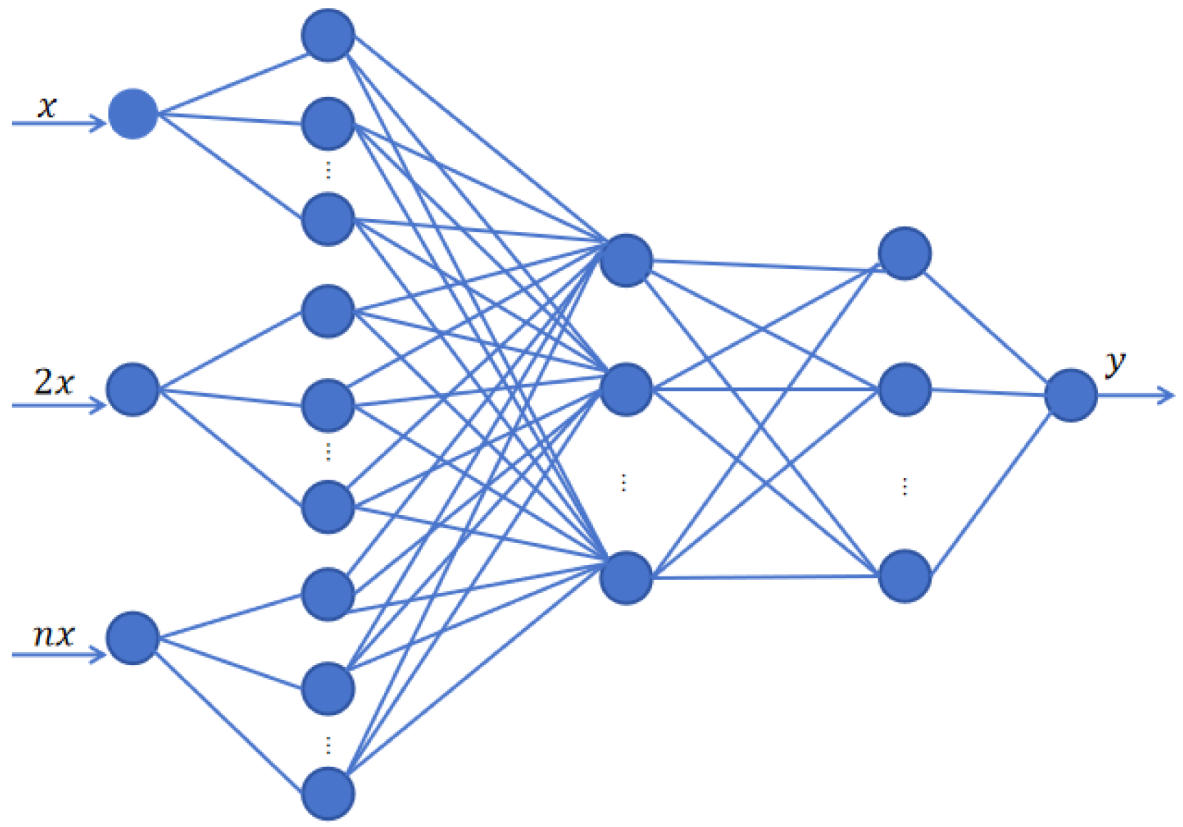
The F-Principle elucidates the phenomenon where neural networks are susceptible to high-frequency catastrophes, which pose significant challenges to training and generalization that are not readily mitigated by mere adjustments of parameters [32]. Employing a sequence of $a_i$ values, extending from 1 to a big number, allows for the construction of a Mscale-DNN framework. This structure is instrumental in enhancing the convergence pace for solutions that span a broad spectrum of frequencies, maintaining consistent precision across these frequencies. The Mscale-DNN network structure is shown in Figure 1.

Figure 1. Mscale-DNN.

3.2. Domain Adaptation in Transfer Learning for PINN

As a well-established research branch in machine learning, domain adaptation essentially addresses the problem of “cross-domain knowledge transfer”. Specifically, when the “source domain” and “target domain” are correlated but differ in data distribution, it enables the knowledge trained on the source domain to be effectively adapted to the target domain through methods such as feature alignment and distribution matching. This logical framework is perfectly applicable to our work: each subproblem we handle can be clearly defined as the ”source domain” and ”target domain” within this framework. In the context of solving partial differential equations (PDEs), to avoid solution discontinuities (e.g., jumps in the solution field at the boundary of source and target domains), we introduce a source domain supervision term into the target domain’s loss function. This facilitates the transfer and alignment of features or knowledge of solutions between subdomains, thereby stabilizing training and improving the overall solution accuracy.

The main idea of domain adaptation in transfer learning for PINNs is to transform the anisotropic problem into several small-scale subproblems. The solving process is divided into two stages. In the initial stage, a traditional PINN is used to obtain the solution to the initial subproblem. In particular, Equation (1) undergoes training over the temporal interval $[0,T_p]$ or the spatial domain $[x_0,x_1]$, employing the conventional PINN approach. The duration of the training interval for the source domain is an adjustable parameter, with its determination being contingent upon the specific problem at hand. In the transfer learning stage, the traditional PINN containing the training information from the previous step is used to solve the problem step by step in a time domain expansion or spatial domain expansion manner. This improved PINN can avoid the problem of traditional PINNs getting stuck in local optima. In the source domain training phase, the dataset $S_p$ is composed of pairs $\{o_{ip},o_{rp}\}$, defined as

$$\begin{array}{cc}\hfill o_{ip}& ={\left\{\left(x_i,\mathcal{I}\left(x_i\right)\right)\mid x_i\in \Omega \right\}}_{i=1}^{N_{ip}},\hfill \\ \hfill o_{rp}& ={\left\{\left(t_i,x_i\right)\mid \left(t_i,x_i\right)\in \left(0,T_p\right]\times \Omega \right\}}_{i=1}^{N_{rp}},\hfill \\ \hfill or{o}_{ip}& ={\left\{\left(x_i,\mathcal{I}\left(x_i\right)\right)\mid x_i\in {\Omega }_p\right\}}_{i=1}^{N_{ip}},\hfill \\ \hfill o_{rp}& ={\left\{\left(t_i,x_i\right)\mid \left(t_i,x_i\right)\in \left(0,T\right]\times {\Omega }_p\right\}}_{i=1}^{N_{rp}},\hfill \end{array}$$

where $N_{rp}$ and $N_{ip}$ are the numbers of residual data and boundary data in the source domain training step, respectively. The formulation of the optimization problem for training in the source domain is restated as follows:

$${\theta }_p=arg\underset{\theta }{min}\mathcal{J}\left(\theta ;S_p\right),$$

(6)

The parameter $\theta$ is typically initialized randomly in the process of solving Equation (5). During formal training, the inclusion of additional supervised information can enhance the performance of the PINN [33]. The solution derived from training within the source domain during the initial phase is utilized as additional supervised learning data for subsequent formal training sessions. The loss function is delineated as follows:

$$\mathcal{J}\left(\theta ;S,{\theta }_p,o_{sp}\right)=\mathcal{J}(\theta ;S)+w_{sp}{\mathcal{J}}_{sp}\left(\theta ;{\theta }_p,o_{sp}\right),$$

(7)

where $w_{sp}$ represents the weight of the extra supervised learning component. The dataset S is composed of pairs $\{o_i,o_r\}$ and defined as

$$\begin{array}{cc}\hfill o_i& ={\left\{\left(x_i,\mathcal{I}\left(x_i\right)\right)\mid x_i\in \Omega \right\}}_{i=1}^{N_i},\hfill \\ \hfill o_r& ={\left\{\left(t_i,x_i\right)\mid \left(t_i,x_i\right)\in \left(0,T\right]\times \Omega \right\}}_{i=1}^{N_r},\hfill \end{array}$$

${\mathcal{J}}_{sp}$ denotes the loss function of supervised learning, defined as

$${\mathcal{J}}_{sp}\left(\theta ;{\theta }_p,o_{sp}\right)={\displaystyle \frac{1}{N_{sp}}}\sum _{i=1}^{N_{sp}}{\left|{\varphi }_{\theta }\left(t_i,x_i\right)-{\varphi }_{{\theta }_p}\left(t_i,x_i\right)\right|}^2$$

with the dataset $o_{sp}$ defined by

$$o_{sp}={\left\{\left(t_i,x_i,{\varphi }_{{\theta }_p}\left(t_i,x_i\right)\right)\mid \left(t_i,x_i\right)\in \left(0,T\right]\times {\Omega }_p\right\}}_{i=1}^{N_{sp}}$$

or

$$o_{sp}={\left\{\left(t_i,x_i,{\varphi }_{{\theta }_p}\left(t_i,x_i\right)\right)\mid \left(t_i,x_i\right)\in \left(0,T_p\right]\times \Omega \right\}}_{i=1}^{N_{sp}},$$

and $N_{sp}$ represents the number of points in the dataset. The optimization problem

$$\overline{\theta }=arg\underset{\theta }{min}\mathcal{J}\left(\theta ;S,{\theta }_p,o_{sp}\right)$$

is solved to derive a numerical solution ${\varphi }_{\overline{\theta }}(t,x)$ for Equation (1) within the domain $\Omega \times (0,T]$. The specific steps of the algorithm can be found in Algorithm 1.

Remark 1. 

The concept of incorporating additional supervised data is closely linked to the label propagation technique [25], and the augmentation of supervised learning contributes to enhancing training performance. This technique demonstrates greater prominence in addressing complex problems, a phenomenon validated by the numerical examples in this study.

Algorithm 1: Domain adaptation for PINNs

Input: Neural network structure; source task; target task. Step 1: Set training steps K, Neural network parameters initialization; Step 2: Incorporate physical laws into the design of the neural network’s loss function $\mathcal{J}\left({\theta }_p,t,x\right)$ based on (5). Solve the source task optimization problem (6) in the first stage. Output the neural network parameters ${\theta }_p$; Step 3: Domain adaptation: Generate the supervised learning data $o_{sp}$ and the training set $S_p$ in next interval; Employ the parameter ${\theta }_p$ of the neural network, obtained upon the conclusion of the preceding training phase, as the initial estimate for the optimization of Equation (7). $\overline{\theta }=arg{min}_{\theta }\mathcal{J}\left(\theta ;S,{\theta }_p,o_{sp}\right)$. output: The approximate solution $ANN(t,x,\overline{\theta })$ of PDE.

3.3. Optimization Method

We seek to find ${\theta }_q$, which minimizes the loss function $\mathcal{J}\left({\theta }_q\right)$. Numerous optimization algorithms exist for minimizing the loss function, with gradient-based optimization techniques commonly utilized in the parameter training process. In the basic form, given an initial value of parameters ${\theta }_q$, $q=1,2,\cdots ,N_{sd}$ is the number of training subintervals. The parameters are updated as

$${\theta }_q^{m+1}={\theta }_q^m-{\left.{\eta }_l{\displaystyle \frac{\partial \mathcal{J}\left({\theta }_q\right)}{\partial {\theta }_q}}\right|}_{{\theta }_q={\theta }_q^m},$$

stochastic Gradient Descent (SGD) represents a prevalent optimization method, where subsets of data points are randomly chosen to approximate the gradient direction in each iteration. This method proves effective in circumventing poor local minima during the training of deep neural networks, particularly under the one-point convexity condition.

3.4. Error Analysis

Define F as the set of functions representing a specified neural network architecture, and let $\varphi$ denote the exact solution to the partial differential equation under consideration. Then, we define ${\varphi }_a=arg{min}_{f\in F}∥f-\varphi ∥$ as the best approximation to the exact solution $\varphi$. Let ${\varphi }_t=arg{min}_{\theta }\mid \mathcal{J}\left(\theta \right)\mid$ be the solution obtained by the training net and ${\varphi }_g=arg{min}_{\theta }\mathcal{J}\left(\theta \right)$ be the solution of the net at the global minimum. Therefore, the total error consists of an approximation error ${\mathcal{E}}_{\mathrm{app}}=∥\varphi -{\varphi }_a∥,$ the generalization error ${\mathcal{E}}_{\mathrm{gen}}=∥{\varphi }_g-{\varphi }_a∥,$ and the optimization error ${\mathcal{E}}_{\mathrm{opt}}=∥{\varphi }_t-{\varphi }_g∥.$ Enhanced network expressivity in a deep neural network can effectively reduce the approximation error, yet it may lead to a substantial generalization error, characterized by the bias–variance trade-off. Within the PINN framework, the number and distribution of residual points play pivotal roles in determining the generalization error, potentially influencing the loss function configuration—especially when employing a sparse set of residual points near steep solution changes. The optimization error stems from the intricate nature of the loss function, with factors such as network structure (depth, width, and connections) exerting significant influence. Fine-tuning hyperparameters like learning rate and number of iterations can further refine and mitigate optimization errors in the network. We have

$${\mathcal{E}}_{PINN}:=∥{\varphi }_t-\varphi ∥\le ∥{\varphi }_t-{\varphi }_g∥+∥{\varphi }_g-{\varphi }_a∥+∥{\varphi }_a-\varphi ∥.$$

3.5. Advantages of PINN Method for Transfer Learning

• In this method, the incorporation of an additional supervised learning component enhances training performance and contributes to a reduction in computational time.
• The methods can decrease the approximation error by employing multi-scale neural networks, which capture high-frequency information.
• This improved PINN avoids the problem of traditional PINNs getting stuck in local optima, thereby reducing optimization errors.

4. Numerical Examples

In this section, we provide multiple numerical illustrations encompassing the Fornberg–Whitham and the modified Fornberg–Whitham equations to show the effectiveness of domain adaptation in transfer learning for PINNs. To demonstrate the feasibility of the proposed algorithm, the baseline PINN method is first used to solve the forward and inverse problems of the Fornberg–Whitham equation, and hyperparameters are analyzed. Then, the improved PINN method is used to improve the boundary error of the region, and the proposed method is tested to have good effects on anisotropic problems. Next, the modified Fornberg–Whitham equation is tested, and the proposed method can obtain higher accuracy numerical results in a shorter time.

To evaluate the performance of our methods, we adopt the relative $L_2$ error. The methodology is implemented within TensorFlow version 1.3, with variables of the float32 data type. Throughout the experiments, the Swish activation function is utilized. For the Adam optimizer, an exponential decay in the learning rate is set to occur every 50 steps with a decay rate of 0.98. The configuration and termination conditions for the L-BFGS optimizer adhere to the recommendations provided in [34]. Prior to initiation of the training phase, neural network parameters are randomly determined following the Xavier initialization method, as outlined in [35].

$${\parallel \epsilon \parallel }_2={\displaystyle \frac{\sqrt{{\sum }_{i=1}^N{\left|{\varphi }_{\theta }\left(t_i,x_i\right)-\varphi \left(t_i,x_i\right)\right|}^2}}{\sqrt{{\sum }_{i=1}^N{\left|\varphi \left(t_i,x_i\right)\right|}^2}}},$$

where $\varphi \left(t_i,x_i\right)$ represents either the actual solution or the reference solution, and ${\varphi }_{\theta }\left(t_i,x_i\right)$ denotes the prediction made by the neural network for a point within the test data ${\left.\left\{\left(t_i,x_i\right)\in (0,T]\times \Omega \right)\right\}}_{i=1}^N$. The test data are formulated through the stochastic sampling of points from the spatiotemporal domain. The performance of the neural network is evaluated using the $L_1$-error

$$\begin{array}{cc}& {\parallel e\parallel }_1={\displaystyle \frac{1}{N}}\sum _{i=1}^N\left|{\varphi }_{\theta }\left(t_i,x_i\right)-\varphi \left(t_i,x_i\right)\right|.\hfill \end{array}$$

4.1. Fornberg–Whitham Equation

Consider Equation (1) with the following initial condition:

$$\varphi (x,0)={\displaystyle \frac{4}{3}}{e}^{\left({\displaystyle \frac{1}{2}}x\right)}.$$

We have the exact solution:

$$\varphi (x,t)={\displaystyle \frac{4}{3}}{e}^{({\displaystyle \frac{1}{2}}x-{\displaystyle \frac{2}{3}}t)}.$$

The computation is carried out in the domain of $-5\le x\le 5$ and $0\le t\le 0.1$. In this assessment, a four-layer fully connected network architecture is employed, featuring 50 neurons in each layer and utilizing the Swish activation function. We also investigate the performance of PINNs with respect to the number of sampling points and boundary points. Specifically, the number of points selected for the trials shown is $N_0=1000,N_f=2000$. We also determine the optimization strategy. Applying the Adam optimizer to optimize the initial trainable parameters in the neural network. Subsequently, the L-BFGS-B optimizer is deployed to fine-tune the neural network, aiming to achieve higher accuracy. The termination of the L-BFGS-B training process is automatically governed by a predefined increment tolerance. Unless otherwise specified, all experiments in this study adopt the following unified setup and parameter configurations to ensure consistency and reproducibility of results.

4.1.1. Baseline PINN

In this section, we evaluate the performance of the baseline PINN method in data-driven solutions of the Fornberg–Whitham equation and data-driven discovery of Fornberg–Whitham equation. We systematically analyze various hyperparameters within the PINN framework to better understand their influence on the predictive accuracy and overall performance of the model.

Firstly, consider the issue of data-driven solutions to the FW equation. Figure 2 encapsulates our findings regarding the data-driven solution to the FW equation. We see that the predicted solution is consistent with the true solution, and the error between the predicted solution and the true solution is small enough. It is feasible to solve the FW equation by the PINN method. With merely a limited set of initial data, the physics-informed neural network effectively grasps the complex nonlinear dynamics inherent in FW equation. This aspect is famously challenging to resolve with precision using conventional numerical techniques, necessitating a meticulous spatial and temporal discretization of the equation. To further evaluate the efficacy of our proposed method, we conduct a series of systematic investigations to measure its predictive accuracy across varying numbers of training and collocation points, as well as different neural network architectures. The relative $L_2$ errors associated with different quantities of initial and boundary training data $N_{\varphi }$ and various numbers of collocation points $N_f$ are detailed in Table 1. The observed trend clearly demonstrates an improvement in predictive accuracy with an augmentation in the quantity of training data $N_{\varphi }$, contingent upon an adequate count of collocation points $N_f$. This finding accentuates a principal advantage of physics-informed neural networks: the incorporation of the inherent structure of the physical laws via collocation points $N_f$ facilitates a learning algorithm that is both more precise and efficient in terms of data utilization. Finally, Table 2 presents the relative $L_2$ errors derived from varying the number of hidden layers and the number of neurons per layer, whilst maintaining constant the number of initial training points and collocation points at $N_{\varphi }=1000$ and $N_f=2000$, respectively.

Figure 2. (Left): Plot of the approximation $\varphi (x,t)$ via the PINN. (Middle): Plot of the exact $\varphi (x,t)$. (Right): Error graph between the exact solution and the predicted solution.

Table 1. The relative $L_2$ norm error between the predicted ${\varphi }_{\theta }$ and the exact solution $\varphi$ across various quantities of initial and boundary training data $N_{\varphi }$, and differing numbers of collocation points $N_f$.

	2000	5000	10,000
200	2.530 $\times {10}^{-3}$	1.101 $\times {10}^{-3}$	1.765 $\times {10}^{-3}$
1000	9.259 $\times {10}^{-5}$	1.030 $\times {10}^{-3}$	3.465 $\times {10}^{-4}$
2000	8.745 $\times {10}^{-4}$	1.277 $\times {10}^{-4}$	6.421 $\times {10}^{-4}$
5000	7.241 $\times {10}^{-4}$	1.385 $\times {10}^{-3}$	4.621 $\times {10}^{-3}$

Table 2. The relative $L_2$ norm discrepancy between the predicted output and the exact $\varphi$ is evaluated in the context of varying numbers of hidden layers and neurons per layer, while maintaining a constant total of training and collocation points at $N_{\varphi }=2000$ and $N_f=3000$, respectively.

	20	30	40	50
1	2.986 $\times {10}^{-4}$	2.903 $\times {10}^{-3}$	3.275 $\times {10}^{-3}$	6.885 $\times {10}^{-4}$
2	4.904 $\times {10}^{-4}$	8.799 $\times {10}^{-5}$	2.814 $\times {10}^{-4}$	7.358 $\times {10}^{-4}$
3	3.961 $\times {10}^{-4}$	4.903 $\times {10}^{-4}$	5.168 $\times {10}^{-4}$	1.778 $\times {10}^{-3}$
4	2.808 $\times {10}^{-4}$	4.339 $\times {10}^{-4}$	4.687 $\times {10}^{-4}$	9.252 $\times {10}^{-5}$

4.1.2. Multiple DA-PINN

Although the PINN method has shown feasibility in solving the forward problem of the FW equation, it may not always achieve the necessary accuracy, especially at the termination time of T = 0.1. Therefore, we attempt to use DA-PINN to solve the above problems, as described in Section 3 as a more appropriate approach to tackle this issue. Specifically, in the DA-PINN process, set the source domain to ($T=0.1$, $x_1=-3$, $x_2=3$) and the target domain to ($T=0.1,x_1=-5,x_2=5$).

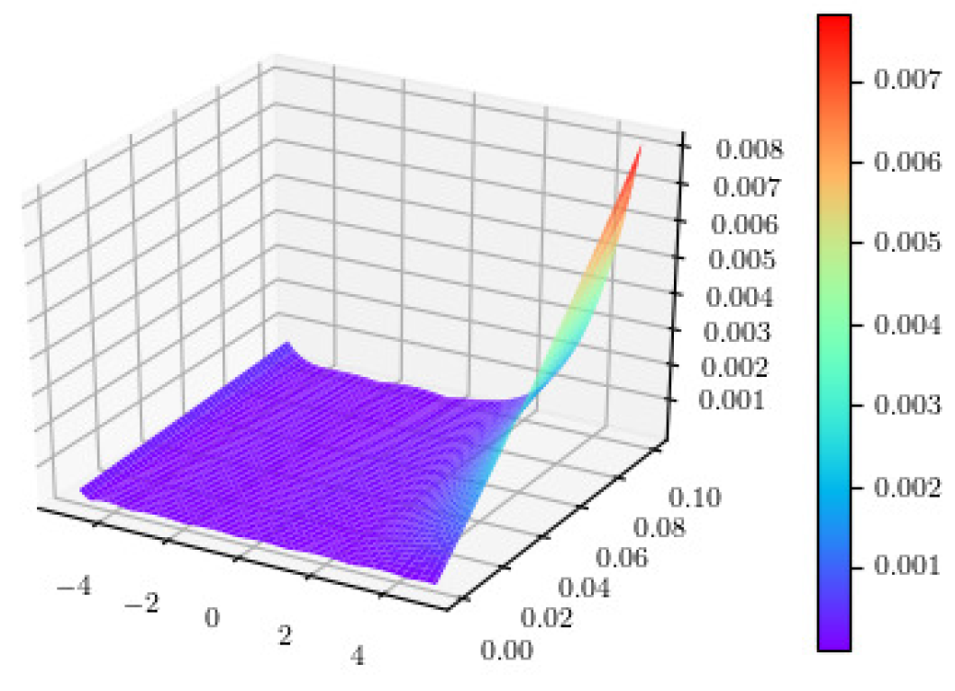
The results obtained demonstrate that the relative $L_2$ error of DA-PINN on the test set is 4.051218 $\times {10}^{-5}$, which is significantly lower compared to the relative $L_2$ error of 8.7981 $\times {10}^{-5}$ obtained when using the PINN method. Furthermore, Figure 3 and Figure 4 illustrate error distribution of two methods. Specifically, the data from the figures reveal that the errors at T = 0.1 generated by DA-PINN are substantially smaller than the corresponding errors at T = 0.1 obtained using the PINN. This underscores the superior precision and effectiveness of the DA-PINN method for addressing the FW equation compared to the standard PINN approach. The $L_1$ Error of the numerical solution of Equation (1) solved by DA-PINN under different spatiotemporal slices is shown in Table 3.

Figure 3. Distribution of absolute errors of the numerical solution by PINN for Fornberg–Whitham equation.

Figure 4. Distribution of absolute errors of the numerical solution obtained by DA-PINN.

Table 3. $L_1$ Errors of the numerical solution for Equation (1) solved by DA-PINN under different spatiotemporal slices.

	x = −5	x = 0	x = 2.5	x = 5
t = 0.02	2.212 $\times {10}^{-4}$	3.411 $\times {10}^{-5}$	3.411 $\times {10}^{-5}$	8.665 $\times {10}^{-5}$
t = 0.04	3.807 $\times {10}^{-4}$	5.254 $\times {10}^{-5}$	3.214 $\times {10}^{-5}$	8.321 $\times {10}^{-5}$
t = 0.06	6.207 $\times {10}^{-4}$	6.578 $\times {10}^{-5}$	7.214 $\times {10}^{-5}$	4.621 $\times {10}^{-4}$
t = 0.08	7.303 $\times {10}^{-4}$	6.374 $\times {10}^{-5}$	7.413 $\times {10}^{-5}$	3.411 $\times {10}^{-4}$
t = 0.1	8.236 $\times {10}^{-4}$	7.417 $\times {10}^{-5}$	8.912 $\times {10}^{-5}$	1.665 $\times {10}^{-3}$

Next, consider the following issues: $x_1=-10$, $x_2=10$, and $T=0.1$. To maintain the precision of the source task, it is essential that the length of the source task interval remains reasonably short. Yet, in more challenging scenarios, a sole source target accompanied by a brief pre-training period might fall short of offering an adequate preliminary estimate for the substantive training phase. To address this issue, we introduce a strategy encompassing multiple instances of transfer learning. This strategy entails the implementation of various transfer learning phases, as outlined below:

$$\left[-x_1,x_1\right],\left[-x_2,x_2\right],\cdots ,\left[-x_{k+1},x_{k+1}\right],\mathrm{with}{x}_1<x_2<\cdots <x_{k+1}=x.$$

in the first transfer learning interval $\left[-x_1,x_1\right]$, the standard transfer learning step is reused. The resulting parameters of the neural network are indicated by ${\theta }_p^{\left(1\right)}$. The transfer learning dataset for the i-th interval is represented by $S_p^{\left(i\right)}$. In any transfer learning interval $\left[-x_i,x_i\right]$, $i>1$, consider the following optimization problem:

$${\theta }_p^{\left(i\right)}=arg\underset{\theta }{min}\mathcal{J}\left(\theta ;S_p^{\left(i\right)},{\theta }_p^{(i-1)},o_p^{(i-1)}\right).$$

The training set of two methods is listed in Table 4.

Table 4. The training sets of the PINN, the 1-interval DA-PINN, and the 2-interval DA-PINN for Equation (1).

Method	Spatial Domain	Nr, Ni, Nsp
PINN	$\left[-10,10\right]$	2000, 1000, -
DA-PINN(1-interval)	$\left[-3,3\right],\left[-10,10\right]$	10,000, 1000, 2000
DA-PINN(2-interval)	$\left[-3,3\right],\left[-5,5\right],\left[-10,10\right]$	10,000, 1000, 2000

In this study, we encounter a problem with $x_1=-10,x_2=10$, and $T=0.1$. To solve this issue, we employ Multiple DA-PINN. However, when using the PINN, we observe a relative $L_2$ error of 6.05 $\times {10}^{-1}$, which indicates that the solution is invalid. In contrast, Multiple DA-PINN produces a relative $L_2$ error of 1.51 $\times {10}^{-3}$, indicating that the solution is valid. Therefore, we conclude that Multiple DA-PINN is a reliable method for solving this particular problem. Our findings demonstrate the effectiveness of Multiple DA-PINN in solving large space issues with high accuracy.

4.1.3. Prediction Results over a Long Time Interval

Given the computational instability encountered when utilizing the standard PINN for long-term evolution simulations, we investigate the potential improvements offered by DA-PINN. The spatial domain for this study is set as [−5, 5], with a time span of T = 20. The relative $L_2$ error for the PINN method in solving this particular problem is measured at 1.27 $\times {10}^{-2}$. In contrast, the relative $L_2$ error for the DA-PINN method in addressing the same issue is notably lower at 2.25 $\times {10}^{-3}$, indicating the effectiveness of the DA-PINN approach in mitigating the aforementioned challenges.

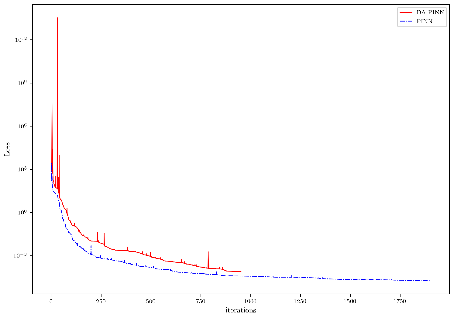
We next evaluate the convergence speed of the proposed method. Figure 5 illustrates the loss convergence of both the PINN and DA-PINN methods. Figure 6 illustrates the relative $L_2$ error of both the PINN and DA-PINN methods. Our results demonstrate that the DA-PINN approach exhibits a faster relative $L_2$ error convergence rate and significantly reduces errors in comparison to the standard PINN method. These findings suggest that DA-PINN provides an effective solution to addressing the numerical instability encountered when utilizing PINNs for long-term evolution simulations. The improved convergence speed of DA-PINN may facilitate better modeling accuracy and reduce computational cost, thus offering a promising avenue for addressing the aforementioned challenges in numerical simulations.

Figure 5. The loss convergence process of PINN and DA-PINN.

Figure 6. The L2 error convergence process of PINN and DA-PINN.

4.2. Data-Driven Discovery of the FW Equation

In this segment of our research, we focus on the task of data-driven discovery of partial differential equations [13]. When the observed partial flow field data of Equation (2) is known and the parameter $\lambda$ is unknown, we can employ the PINN method to reconstruct the complete flow field and infer the unknown parameter $\lambda$. Our approach involves approximating $\varphi (t,x)$ through a deep neural network. Under this framework, together with Equation (2), we derive a physics-informed neural network $f(t,x)$. This derivation is facilitated by employing the chain rule to differentiate function compositions via automatic differentiation. Notably, the differential operator parameters $\lambda$ are assimilated as parameters within the physics-informed neural network $f(t,x)$. Numerical results obtained with the PINN are displayed in Figure 7.

Figure 7. (Top): Plot of the approximation $\varphi (x,t)$ via the PINN. (bottom): Snapshots of the approximation $\varphi (x,t)$ vs. the exact solution at various time points through the temporal evolution.

The objective of our study is to estimate the unknown parameter $\lambda$ even in the presence of noisy data, utilizing the PINN. Table 5 summarizes our findings for this case. Our results demonstrate that the physics-informed neural network accurately identifies the unknown parameter $\lambda$ with high precision, even in the presence of noisy training data. Specifically, the estimation error for $\lambda$ is 0.44% under noise-free conditions and 0.55% when training data are corrupted by 1% uncorrelated Gaussian noise.

Table 5. Relative $L_2$ errors of the approximate solution for Equation (2) with clean data and noisy data.

	Error $\mathit{\varphi }$	Error $\mathit{\lambda }$
Clean data	2.983 $\times {10}^{-5}$	0.02298%
Noise data	6.782 $\times {10}^{-4}$	0.91528%

The Mscale-PINN method is an improved version of the PINN method that enhances solution accuracy by introducing an adaptive scale parameter in the first layer of the network structure. To conduct the comparison, both the Mscale-PINN model and the traditional PINN model are trained using the same dataset and training procedure, with the $L_2$ error serving as the evaluation metric. A summary of our results for this example is presented in Table 6. Experimental results demonstrate that the Mscale-PINN method achieves lower relative $L_2$ error compared to the traditional PINN method when solving Equation (2). Further analysis reveals that the Mscale-PINN method, by dynamically adjusting the scale parameter, adapts better to the physical processes at different scales, thereby providing more accurate solutions.

Table 6. Comparison of relative $L_2$ errors between Mscale-PINN and PINN in solving Equation (2).

	Error $\mathit{\varphi }$	Error $\mathit{\lambda }$
Mscale-PINN	2.623 $\times {10}^{-5}$	0.00026%
PINN	2.982 $\times {10}^{-5}$	0.02298%

4.3. Modified Fornberg–Whitham Equation

In this section, we compare the proposed DA-PINN method with the variational iteration method (VIM) [31], as well as the baseline PINN. The VIM is an analytical approximation technique that solves nonlinear differential equations iteratively by constructing correction functionals to establish a reference from traditional numerical methods. As a well-established numerical scheme, the VIM provides solutions with high accuracy within its convergence region and is often used to validate newly proposed numerical methods. Its results can be regarded as a ‘quasi-exact’ solution, allowing for a fair assessment of the accuracy of different numerical approaches. For this example, consider Equation (3) subject to the following initial condition:

$$\varphi (x,0)={\displaystyle \frac{3}{4}}(\sqrt{15}-5){sech}^2\left(cx\right),$$

where c is the wave speed given by

$$c={\displaystyle \frac{1}{20}}\sqrt{\left(10(5-\sqrt{15})\right)},$$

and the corresponding exact solution is

$$\varphi (x,t)={\displaystyle \frac{3}{4}}(\sqrt{15}-5){sech}^2\left(c(x-(5-\sqrt{15})t)\right).$$

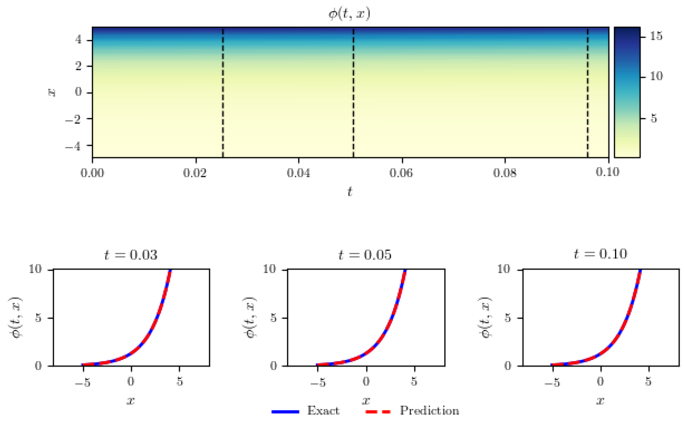
The solution region for this problem is [−5, 5], with T = 0.1. The efficacy and applicability of DA-PINN for the current problem are presented in Table 7, showing the absolute error of $\varphi$ for different values of t and x. The data presented in the tables demonstrate that the absolute errors produced by DA-PINN are considerably lower than those generated using the VIM [31]. The characteristics of both exact and approximated solutions are depicted in Figure 8 and Figure 9.

Table 7. $L_1$ error for VIM, PINN, and DA-PINN for Equation (3) when x = 2.5.

	VIM	PINN	DA-PINN
t = 0.02	1.180 $\times {10}^{-4}$	2.911 $\times {10}^{-5}$	1.305 $\times {10}^{-5}$
t = 0.04	2.363 $\times {10}^{-4}$	3.614 $\times {10}^{-5}$	1.842 $\times {10}^{-5}$
t = 0.08	4.731 $\times {10}^{-4}$	4.413 $\times {10}^{-5}$	2.034 $\times {10}^{-5}$
t = 0.1	5.914 $\times {10}^{-4}$	3.912 $\times {10}^{-5}$	2.265 $\times {10}^{-5}$

Figure 8. Contrast exact solution (middle) $\varphi (t,x)$ for Equation (3) with the result obtained by DA-PINN (left) based on the numerical error (right).

Figure 9. Visual representations of the approximation $\varphi (x,t)$ compared to the high-fidelity solution are depicted at various time points throughout its temporal evolution for Equation (3).

4.3.1. The Problem of Large Space–Time Domain

In the subsequent analysis, we expand our research to a larger spatiotemporal domain, namely $[-20,20]\times [0,10]$. This expansion enables us to assess the performance of Multiple DA-PINN in handling problems of increasing complexity. By applying Multiple DA-PINN to this extended domain, we aim to ascertain its efficacy in capturing spatiotemporal dynamics in larger-scale problems. The relative error of solving this problem with the multiple DA-PINN method is 8.578 $\times {10}^{-4}$, which is 82% lower than that calculated with the baseline PINN method.

We see in Figure 10 that the DA-PINN prediction is very accurate and indistinguishable from the exact solution. For the test problem, the absolute errors are conveyed in Table 8 for different values of t and x.

Figure 10. Figure of numerical and exact solutions of Equation (3) solved by DA-PINN in the spatiotemporal domain $[-20,20]\times [0,10]$.

Table 8. $L_1$ errors of Equation (3) estimated by DA-PINN at various time scales.

	x = −5	x = 2.5	x = 5
t = 2	6.212 $\times {10}^{-4}$	1.411 $\times {10}^{-4}$	1.665 $\times {10}^{-5}$
t = 4	1.207 $\times {10}^{-3}$	3.214 $\times {10}^{-4}$	4.621 $\times {10}^{-4}$
t = 8	1.303 $\times {10}^{-3}$	4.413 $\times {10}^{-4}$	1.411 $\times {10}^{-4}$
t = 10	7.236 $\times {10}^{-3}$	3.912 $\times {10}^{-4}$	4.665 $\times {10}^{-4}$

4.3.2. Ablation Analysis Experiments

To systematically evaluate the contribution of each component in the proposed DA-PINN method and its sensitivity to key hyperparameters, a series of ablation and sensitivity experiments are conducted in this section. All experiments are performed on the Fornberg–Whitham equation introduced in Section 4.2. The primary goal of these experiments is to isolate the two core components of the DA-PINN framework—domain adaptation and the multi-scale structure (Mscale-DNN)—to verify their necessity. 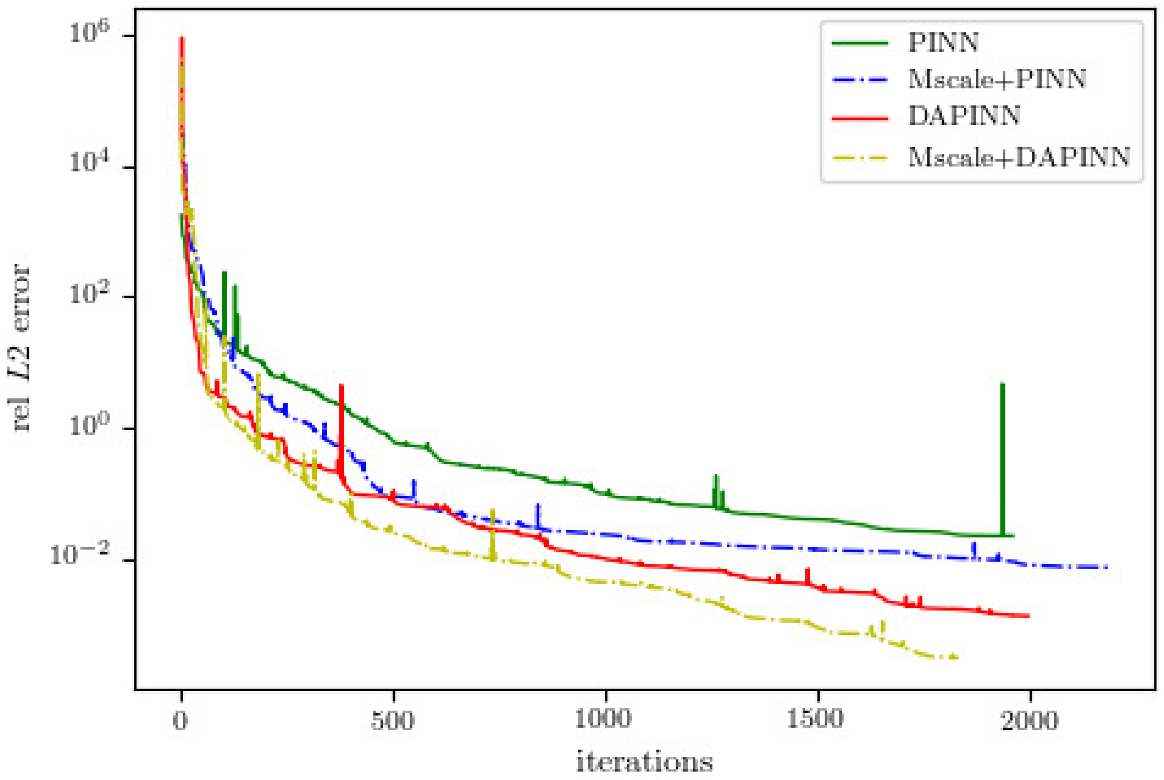Under the settings of spatiotemporal domain $[-30,30]\times [0,15]$, four model configurations are compared: (a) Baseline PINN: The standard PINN method. (b) PINN + Mscale: Utilizing only the multi-scale network structure without domain adaptation. (c) DAPINN (ours): Employing domain adaptation with a standard fully connected neural network structure. (d) DAPINN + Mscale: Our complete proposed model, integrating both domain adaptation and the multi-scale network structure.

The relative $L_2$ error is adopted as the evaluation metric, and the results are presented in Table 9. The convergence process of relative L2 error is shown in Figure 11.

Table 9. Ablation study on relative $L_2$ errors of different model configurations.

Model Configurations	PINN	PINN + Mscale	DAPINN	DAPINN + Mscale
Relative $L_2$ Error	6.05 $\times {10}^{-2}$	4.82 $\times {10}^{-2}$	2.51 $\times {10}^{-3}$	9.74 $\times {10}^{-4}$
Time (s)	1603	1723	1689	1556

Figure 11. The descending curves of $L_2$ errors under the four configurations in the spatiotemporal domain $[-30,30]\times [0,15]$.

It is evident from the results that introducing transfer learning yields an order-of-magnitude improvement in accuracy. This indicates that for problems with a certain spatial scale, decomposing complex tasks via domain adaptation strategies is crucial for enhancing PINN performance. Regarding the multi-scale structure, its standalone application brings limited improvements. However, when combined with transfer learning, it further enhances accuracy. This suggests that Mscale-DNN effectively improves the model’s expressive capacity, enabling better fitting of high-frequency components of the solution, thus forming a strong complement to the domain adaptation strategy.

5. Conclusions

In this study, we propose the domain adaptation in transfer learning for PINN (DA-PINN) method for solving Fornberg–Whitham type equations. This study represents the inaugural endeavor to employ neural networks for solving the FW equation. Our results demonstrate the feasibility of using the neural networks to solve the FW equation, particularly excelling in inverse FW problems. The integration of transfer learning strategies within the PINN framework significantly enhances training effectiveness. For larger spatiotemporal scales, DA-PINN serves as a viable solution when PINNs fail. Our method effectively alleviates the issue of becoming trapped in local optima during optimization, thus enhancing predictive accuracy. Moreover, it is effective in accelerating loss convergence and reducing computational time for long-term predictive scenarios. Compared to traditional VIM methods, DA-PINN exhibits higher accuracy in solving the modified FW equation, highlighting the potential of our proposed approach in numerically solving the FW equation.