Dynamic Equilibria with Nonsmooth Utilities and Stocks: An L^∞ Differential GQVI Approach

Abstract

We develop a comprehensive dynamic Walrasian framework entirely in $L^{\infty }$ so that prices and allocations are essentially bounded, and market clearing holds pointwise almost everywhere. Utilities are allowed to be locally Lipschitz and quasi-concave; we employ Clarke subgradients to derive generalized quasi-variational inequalities (GQVIs). We endogenize inventories through a capital-accumulation constraint, leading to a differential QVI (dQVI). Existence is proved under either strong monotonicity or pseudo-monotonicity and coercivity. We establish Walras’ law, and the complementarity, stability, and sensitivity of the equilibrium correspondence in $L^2$-metrics, incorporate time-discounting and uncertainty into $\Omega \times [0,T]$, and present convergent numerical schemes (Rockafellar–Wets penalties and extragradient). Our results close the “in mean vs pointwise” gap noted in dynamic models and connect to modern decomposition approaches for QVIs.

1. Introduction

The variational inequality (VI/QVI/GQVI) approach to competitive equilibrium (see, e.g., [1] and references therein) is a practical alternative to fixed-point methods [2,3,4]. In dynamic $L^p$ models ($1\le p<\infty$), however, feasibility is encoded by integrals, so one usually obtains only clearing in mean. This leaves open two questions: do markets clear a.e. in time, and does complementarity hold pointwise? We answer both by working in $L^{\infty }$. Our framework delivers a.e. clearing and complementarity and still handles locally Lipschitz, quasi-concave utilities, inventory dynamics with discounting, uncertainty, and provably convergent algorithms.

$L^{\infty }$ is a natural setting in continuous time: (i) prices and consumptions are bounded; (ii) budgets use the $L^{\infty }$-$L^1$ pairing; and (iii) the price simplex is weak-∗ compact (Banach–Alaoglu). This compactness yields existence without extra compactifications. Testing against simple prices then turns integral inequalities into pointwise complementarity and produces a.e. clearing.

We organize our main results around seven themes that advance the dynamic Walrasian VI/QVI/GQVI literature:

(C1)

Functional setting in $L^{\infty }$. Prices and allocations live in $L^{\infty }\left(\mathcal{T}\right)$; the price set is a weak-∗ compact simplex and budget sets are weak-∗ compact bands. The existence of equilibrium follows without additional price compactifications, and we obtain a.e. market clearing and complementarity by a simple-function testing argument.

(C2)

From “in mean” to a.e. clearing. We prove that solutions of the master VI against the convex hull of simple price functions imply ${\sum }_a(x_a^{\left(j\right)}-e_a^{\left(j\right)})\le 0$ and ${\overline{p}}^{\left(j\right)}·{\sum }_a(x_a^{\left(j\right)}-e_a^{\left(j\right)})=0$ a.e. for each good j. This closes the gap noted in dynamic $L^p$ models where only integral clearing was available.

(C3)

Nonsmooth utilities and GQVI. Allowing locally Lipschitz, quasi-concave instantaneous utilities, we formulate household optimality via generalized Vi using Clarke subgradients, relying on measurable selection theorems to obtain measurable subgradient selections and well-posedness of the generalized VI.

(C4)

Production, stockpiling, and dQVI. We introduce inventories through linear capital accumulation with depreciation and show that the joint household–firm–inventory system admits an equilibrium characterized as a differential QVI (dQVI).

(C5)

Qualitative properties. Under strong monotonicity (in an $L^2$ metric) or under pseudo-monotonicity with coercivity, we prove existence; with strong monotonicity we derive Lipschitz stability of the equilibrium correspondence and Walras’ law. These provide regularity and sensitivity results in the spirit of stability analyses for dynamic price VIs.

(C6)

Numerics. We give implementable schemes: Rockafellar–Wets penalty methods to enforce budgets and Korpelevich’s extragradient for the monotone GVI. Under strong monotonicity, we prove linear convergence; in the merely monotone case we obtain $O(1/k)$ ergodic rates. A detailed dynamic Cobb–Douglas example (single- and multi-good) illustrates closed forms, a price fixed-point map, and discretized extragradient updates.

(C7)

Scalability. After time discretization the GQVI decomposes by agents and time slabs. We outline a Dantzig–Wolfe-type master/worker decomposition that aligns with contemporary QVI decomposition frameworks, enabling large-scale computations.

Our analysis builds on and sharpens a line of results that positioned dynamic equilibria within VI/QVI theory. Time-dependent Walrasian formulations and computational procedures were developed for continuous time in variational form (e.g., [5,6,7,8,9,10]), and quasi-variational models for quasi-concave preferences were advanced in [11,12]. Conceptual remarks on Lebesgue-space modeling and the limitations of mean-value clearing appear in [13,14]. Regularity and sensitivity for dynamic price VIs (e.g., [15]) highlighted the importance of monotonicity and stability. On the nonsmooth side, generalized subdifferential tools and measurable selection techniques (e.g., [16,17,18]) allow us to treat locally Lipschitz, quasi-concave utilities in a dynamic GQVI form, complementing the static analyses in [11,12]. For the “evolution” and stability viewpoint, we connect to recent work on equilibrium evolution and stability properties [19]. Algorithmically, we lean on classical extragradient methods [20] and penalty approaches [17], and relate our decomposition discussion to recent QVI master/worker architectures (see, e.g., [21]).

Methodologically, we rely on three devices: weak-∗ compactness in $L^{\infty }$ (for price and band compactness), Mosco convergence of budgets under $L^1$ price changes (for stability of household solutions and continuity of excess demand), and testing against simple prices (to pass from integral inequalities to pointwise complementarity via Lebesgue differentiation). Together, these give a.e. clearing without extra compactifications or restrictive price dynamics. For nonsmooth utilities we adopt Clarke subdifferentials with measurable selections, enabling generalized VI statements while retaining monotonicity (or pseudo-monotonicity) needed for existence and stability.

Conceptually the novelties can be so summarized: (i) our $L^{\infty }$ formulation delivers a.e. clearing and complementarity in continuous time, closing the “in mean vs a.e.” gap for dynamic Walrasian models; (ii) we integrate inventories and stockpiling explicitly via a differential law within a QVI system; (iii) we accommodate locally Lipschitz, quasi-concave utilities and still provide existence and regularity; (iv) we provide constructive, convergent numerical schemes with rates under strong monotonicity; and (v) we connect the theory to scalable decomposition architectures for large agent/time systems.

The rest of this paper is organized as follows. In Section 2 we place our contribution in the variational context on the competitive equilibrium, clarifying how an $L^{\infty }$ formulation changes the economic meaning of feasibility and prices relative to $L^p$ approaches and why almost-everywhere clearing naturally enters the picture. Section 3 then assembles the analytic ingredients that make this perspective workable: topology for prices and allocations, weak-∗ compactness of band sets, continuity of the $L^{\infty }$–$L^1$ pairing, Mosco stability of budgets as prices vary, and the basic measurability needed for Clarke selections. Building on this foundation, Section 4 lays out the economic environment as a single variational object: banded consumption sets and budget hyperplanes for households, box-type production (when present), and, in the dynamic setting, a linear stock law that ties production, consumption, and inventories together. With the model in place, Section 5 develops the core implications of the framework: equilibrium is obtained from a master variational inequality, integral balance is converted into pointwise clearing and complementary slackness by testing with simple prices, robustness is articulated through stability of allocations with respect to prices, and the dynamic and stochastic extensions are treated within the same operator viewpoint. Section 6 develops the computational side of the framework, introducing time discretization and projection/proximal updates, analyzing extragradient and primal–dual splitting with practical stepsize rules (fixed and adaptive), and reporting convergence behavior (ergodic $O(1/k)$ decay in the monotone regime and linear contraction under stronger curvature), together with brief remarks on mesh dependence and per-iteration complexity. Section 7 presents stylized numerical illustrations—first an exchange economy without inventories and then a dQVI with a stock variable—showing how the framework yields almost-everywhere clearing and pointwise complementarity in practice, and how the proposed algorithms behave under discretization. In Section 8, we distill the analytic results into an implementation guide, indicating what data are needed, how to set bounds and stepsizes, and how to interpret the diagnostics in empirical or operational settings. Section 9 closes by reflecting on scope and limitations, highlighting when the $L^{\infty }$ choice is economically essential and outlining directions where the same perspective could be extended, for example, to richer technologies, market designs, or learning-based estimation of primitives.

2. Literature Overview

To situate our contribution within the VI/QVI/GQVI literature on competitive equilibrium, we group works by methodological theme and indicate how our $L^{\infty }$ framework advances each line.

(L1)

Variational formulations of equilibrium. Casting equilibria as VIs/QVIs has roots in classical monotone operator theory and variational analysis; see, among others, [17,22,23]. In the exchange setting, Jofre et al. in [22] formulated price determination as a VI on a convex feasible set, opening a path beyond fixed-point methods. Our analysis follows this route but works entirely in $L^{\infty }$ and moves from integral feasibility to pointwise (a.e.) complementarity.

(L2)

Time-dependent/dynamic Walrasian models. For continuous-time markets, Maugeri and Vitanza in [5] and the series [6,7,8,9,10] developed evolutionary VI/QVI formulations with prices and allocations in Lebesgue spaces, typically obtaining clearing in mean. These papers established existence and computational procedures under various monotonicity assumptions. Our contribution complements this line by proving existence in $L^{\infty }$ and converting the master VI into a.e. complementarity through a simple-function testing device, thereby closing the “in mean vs a.e.” gap.

(L3)

Quasi-concavity, quasi-variational inequalities, and nonsmooth utilities. Allowing quasi-concave utility weakens convexity and naturally leads to QVIs; see [11,12]. Dynamic settings with locally Lipschitz utilities require generalized subdifferentials; we rely on Clarke calculus and measurable selections (cf. [16,17,18]) to formulate household optimality as a generalized VI (GVI) in continuous time. This bridges static QVI treatments with dynamic, nonsmooth preferences (see also [24]).

(L4)

Lebesgue-space modeling and the role of $L^{\infty }$. Conceptual remarks on choosing Lebesgue spaces for dynamic equilibrium and consequences for feasibility appear in [13,14]. When $p\in L^p$ for $p<\infty$, price sets are not compact and clearing emerges only in integral form. By placing prices and consumptions in $L^{\infty }$, we exploit weak-∗ compactness (Banach–Alaoglu) and obtain a.e. clearing via testing on indicator-price simple functions. This shift is the cornerstone of our existence and complementarity results.

(L5)

Contrasting $L^{\infty }$ with $L^p$ dynamic equilibrium models. A central distinction between our framework and prior dynamic Walrasian models lies in the choice of function space for prices and allocations. The influential series by Donato, Milasi, and Vitanza [7,8,9,10] formulates equilibrium in $L^p$ settings ($1\le p<\infty$), where feasibility and market clearing are enforced in integral form—typically yielding clearing in mean. However, $L^p$ spaces lack weak-∗ compactness, and price sets are not closed under pointwise convergence, which complicates existence proofs and limits the granularity of complementarity conditions. By contrast, our $L^{\infty }$ framework leverages Banach–Alaoglu compactness and simple-function testing to achieve almost-everywhere (a.e.) clearing and complementarity. This shift enables pointwise Walras’ law, strong stability results, and a direct formulation of household optimality as a GVI, marking a conceptual and technical advance over $L^p$-based approaches.

(L6)

Production, stockpiling, and dynamic constraints. Production and inventories can be incorporated into dynamic Walrasian models through time-dependent constraints and state equations. Variational formulations for time-dependent equilibria are surveyed in [5]. We formalize inventories through a linear capital-accumulation law with depreciation and derive a differential QVI (dQVI), extending the exchange-only formulations in [8,9,10].

(L7)

Stability, sensitivity, and evolution. Regularity and sensitivity for price-based dynamic VIs are treated in [15]. The broader stability/evolution viewpoint for equilibria has been advanced in [19], which studies how equilibria vary under perturbations and in time. In our framework, strong monotonicity (in an $L^2$ metric) yields Lipschitz dependence of optimal allocations on prices and leads to stability of the aggregate excess map. We also provide a pointwise Walras’ law in the $L^{\infty }$ setting.

(L8)

Stochasticity, discounting, and measurability. Discounting is standard in intertemporal utility and integrates seamlessly in VI formulations (e.g., [8]). For uncertainty on $\Omega \times \mathcal{T}$, measurability issues are handled through Komlós-type subsequences and measurable selections [18,25]. We extend existence and a.e. clearing to the product space, obtaining pointwise complementarity in $(\omega ,t)$.

(L9)

Computational methods. Early computational procedures for time-dependent Walrasian VIs are discussed in [6]. For monotone operators on convex sets, the extragradient method [20] is a robust baseline, while penalty methods provide a principled way to enforce budget and complementarity constraints [17]. We analyze both in our $L^{\infty }$ model and establish linear convergence under strong monotonicity and $O(1/k)$ ergodic rates in the merely monotone case. Our dynamic Cobb–Douglas example offers closed forms and a price fixed-point iteration that is readily discretized.

(L10)

Operator-splitting and primal–dual algorithms (compatibility). The $L^{\infty }$–weak-∗ formulation is compatible with contemporary splitting schemes such as PDHG/Chambolle–Pock, mirror-prox, and ADMM [26,27,28,29]. Two features are decisive: (i) all feasibility pieces (bands, production boxes, price simplex) are convex sets with simple prox/projection operators (pointwise in time); and (ii) the linear state map $K:(x,y,k)\mapsto (Ak-b(x,y\left)\right)$ separates cleanly from the nonsmooth parts, enabling primal–dual updates with diagonal preconditioning. As a result, the same sublinear $O(1/k)$ ergodic gap decay (monotone case) and linear rates under strong curvature/monotonicity extend to the present $L^{\infty }$ framework after discretization, while the economic gains of weak-∗ compactness (existence and a.e. complementarity) are retained. Operational details (prox operators, stepsize rules, and a saddle formulation) are summarized in Section 6 and Section 8.

(L11)

Decomposition and scalability. Network and decomposition ideas for equilibrium computation have a long pedigree (e.g., [30,31,32]). The rise of QVI decomposition is pushing scalability to large agent/time systems; see [21] for a recent Dantzig–Wolfe style architecture for QVIs. After time discretization, our GVI/GQVI separates by agents and time slabs, enabling master–worker price updates and parallel household subproblems, consistent with these decomposition paradigms.

(L12)

Recent operator-splitting and primal–dual algorithms. Beyond classical extragradient and penalty methods, recent advances in operator-splitting (e.g., [27,28]) and primal–dual schemes (e.g., [26,29]) offer scalable solvers for monotone inclusions and saddle-point problems. These methods are particularly suited to large-scale, time-discretized GVI/GQVI systems. While our focus is on existence and structure, the decomposition architecture we propose is compatible with these modern algorithms, and our companion paper explores their application to dynamic equilibrium computation.

The use of $L^{\infty }$ as the basic function space is not only a mathematical device (to gain weak-∗ compactness of bands) but also carries economic meaning. Boundedness of consumption and production streams corresponds to technological, physical, or policy limits that prevent agents from consuming or producing without bound. In contrast, models based on $L^p$ with $1\le p<\infty$ permit unbounded spikes in consumption at negligible measure sets; while analytically convenient in reflexive cases, such spikes are economically implausible if one insists on feasibility at every instant. Thus the $L^{\infty }$ framework better matches markets where resources are capped in real time.

Pointwise complementarity also has a direct interpretation. At almost every $(\omega ,t)$, if the price of good j is strictly positive, then the market for good j clears exactly at that state and time; conversely, if there is excess supply of good j at $(\omega ,t)$, the equilibrium price of that good must vanish there. In practical terms, this means that positive prices serve as indicators of binding scarcity, while goods that are freely available carry zero price. This condition extends the classical notion of market clearing to a pathwise, almost-everywhere statement, aligning with real-time operation in electricity, network, or financial markets where feasibility must hold continuously rather than only in expectation.

In short, the $L^{\infty }$–based formulation preserves existence while delivering a.e. clearing and pointwise complementarity, extends to inventories (dQVI) and uncertainty on product spaces, provides parametric stability of allocations with respect to prices, and admits implementable first-order algorithms (extragradient and primal–dual splitting) with standard rates after discretization.

3. Preliminaries

In this section we collect basic facts on weak-* compactness in $L^{\infty }$, Mosco convergence of budget sets, measurable Clarke subgradients, and a simple testing principle for a.e. inequalities.

3.1. Notation

For $f\in L^{\infty }(\mathcal{T},{\mathbb{R}}^l)$ and $g\in L^1(\mathcal{T},{\mathbb{R}}^l)$ the duality pairing is $⟨f,g⟩={\int }_0^{T}f\left(t\right)·g\left(t\right)dt$. For $x={\left(x_a\right)}_{a=1}^n$ we write ${\parallel x\parallel }_2^2={\sum }_{a=1}^n{\int }_0^T{|x_a\left(t\right)|}^{2}dt$ (an $L^2$ metric used for stability). For a measurable multifunction $M:\mathcal{T}\rightrightarrows {\mathbb{R}}^l$, $\mathrm{gph}M=\left\{\right(t,y):y\in M(t\left)\right\}$.

3.2. Weak-∗ Compactness of Bands

Lemma 1 (Bands are weak-∗ compact).

Let $\overline{x}\in L_{+}^{\infty }(\mathcal{T},{\mathbb{R}}^l)$ and $X=\{x\in L_{+}^{\infty }:0\le x\left(t\right)\le \overline{x}\left(t\right)a.e.\}$. Then X is convex, weak-∗ closed, and weak-∗ compact in $L^{\infty }$.

Proof. 

Convexity and weak-∗ closedness are immediate. Since ${\parallel x\parallel }_{L^{\infty }}\le {\parallel \overline{x}\parallel }_{L^{\infty }}$ on X, weak-∗ compactness follows from the Banach–Alaoglu theorem [33]; see also ([34], Thm. 5.116) for the $L^{\infty }$ case. □

3.3. Mosco Convergence of Budget Sets in $L^{\infty }$

Lemma 2 (Mosco convergence of budget half-spaces).

Fix agent a. Let $p_k\to p$ in $L^1(\mathcal{T},{\mathbb{R}}^l)$ and set $M_a\left(p\right)=\{x\in X_a:⟨p,x-e_a⟩\le 0\}$. Then $M_a\left(p_k\right)\to M_a\left(p\right)$ in the sense of Mosco: (i) (inner limit) for any $x\in M_a\left(p\right)$ there exist $x_k\in M_a\left(p_k\right)$ with $x_k\stackrel{w^{*}}{\to }x$ in $L^{\infty }$; (ii) (outer limit) if $x_k\in M_a\left(p_k\right)$ and $x_k\stackrel{w^{*}}{\to }x$, then $x\in M_a\left(p\right)$.

Proof. 

(i) If $⟨p,x-e_a⟩<0$, then $⟨p_k,x-e_a⟩<0$ for k large, so choose $x_k=x$. If $⟨p,x-e_a⟩=0$, pick ${\theta }_k\downarrow 0$ with $⟨p_k,(1-{\theta }_k)x-e_a⟩\le 0$ (possible because $⟨p_k,x⟩\to ⟨p,x⟩=⟨p,e_a⟩$), and set $x_k=(1-{\theta }_k)x$. Then $x_k\in X_a$ and $x_k\stackrel{w^{*}}{\to }x$. This is a standard application of Mosco convergence of convex sets [16] together with epi/Painlevé–Kuratowski limits for half-spaces ([17], Chs. 11–12). (ii) follows from $⟨p_k,x_k-e_a⟩\le 0$ and $⟨p_k,x_k-e_a⟩\to ⟨p,x-e_a⟩$ by bilinearity and $p_k\to p$ in $L^1$, while $x_k\stackrel{w^{*}}{\to }x$ in $L^{\infty }$. □

Remark 1.

As prices $p_k\to p$ in $L^1$, the linear budget inequality $⟨p_k,x-e_a⟩\le 0$ defines half-spaces that “tilt” continuously in the weak-∗ geometry of the band $X_a$: if a plan x is feasible at p, nearby prices keep it feasible up to an arbitrarily small rescaling, and any weak-∗ limit of feasible plans at $p_k$ remains feasible at p. Equivalently, the admissible region $M_a\left(p_k\right)=X_a\cap \{⟨p_k,x-e_a⟩\le 0\}$ varies in a way that preserves both inner feasibility (you can approximate feasible points) and outer closure (limits of feasible plans stay feasible), which is exactly the content of Mosco convergence.

Lemma 3 (Budget sets are weak-∗ closed and compact in bands).

Fix an agent a and $p\in L^1(\mathcal{T},{\mathbb{R}}^l)$. Let $X_a=\{x\in L_{+}^{\infty }:0\le x\le {\overline{x}}_a\}$ with ${\overline{x}}_a\in L_{+}^{\infty }(\mathcal{T},{\mathbb{R}}^l)$, and ${\displaystyle M_a\left(p\right):=\left\{x\in X_a:⟨p,x-e_a⟩={\int }_0^{T}p\left(t\right)·\left(x\left(t\right)-e_a\left(t\right)\right)dt\le 0\right\}}$.

Then $M_a\left(p\right)$ is weak-∗ closed in $L^{\infty }(\mathcal{T},{\mathbb{R}}^l)$; consequently, $M_a\left(p\right)$ is weak-∗ compact (as a weak-∗ closed subset of the weak-∗ compact band $X_a$).

Proof. 

Let ${\left(x_k\right)}_k\subset M_a\left(p\right)$ and suppose $x_k\stackrel{w^{*}}{\to }x$ in $L^{\infty }$. By definition of weak-∗ convergence, for every $q\in L^1$, $⟨q,x_k⟩\to ⟨q,x⟩$. In particular, with the fixed $q=p$ and the fixed $e_a\in L^{\infty }$,

$$⟨p,x_k-e_a⟩⟶⟨p,x-e_a⟩.$$

Since $⟨p,x_k-e_a⟩\le 0$ for all k, passing to the limit gives $⟨p,x-e_a⟩\le 0$; hence, $x\in M_a\left(p\right)$. Thus, $M_a\left(p\right)$ is weak-∗ closed. Weak-∗ compactness then follows because $X_a$ is weak-∗ compact by Lemma 1 and $M_a\left(p\right)\subseteq X_a$ is weak-∗ closed. □

Lemma 4 (Joint continuity of the $L^{\infty }$–$L^1$ pairing under mixed limits).

Let ${\left(p_k\right)}_k\subset L^1(\mathcal{T},{\mathbb{R}}^l)$ with $p_k\to p$ in $L^1$, and let ${\left(x_k\right)}_k\subset L^{\infty }(\mathcal{T},{\mathbb{R}}^l)$ with $x_k\stackrel{w^{*}}{\to }x$ in $L^{\infty }$. Fix $e\in L^{\infty }(\mathcal{T},{\mathbb{R}}^l)$. Suppose moreover that ${\left(x_k\right)}_k$ is uniformly essentially bounded, e.g., $x_k\in X:=\{x:|x|\le \overline{x}\}$ for some $\overline{x}\in L^{\infty }$. Then

$$⟨p_k,x_k-e⟩⟶⟨p,x-e⟩.$$

Proof. 

Write

$$⟨p_k,x_k-e⟩-⟨p,x-e⟩=\underset{\left(I\right)}{\underbrace{⟨p_k-p,x_k-e⟩}}+\underset{\left(II\right)}{\underbrace{⟨p,x_k-x⟩}}.$$

For $\left(I\right)$, Hölder’s inequality and uniform boundedness give

$$|\left(I\right)|\le \parallel p_k{-p\parallel }_{L^1}\parallel x_k{-e\parallel }_{L^{\infty }}\le {\parallel p_k-p\parallel }_{L^1}\left(\parallel \overline{x}{\parallel }_{L^{\infty }}+{\parallel e\parallel }_{L^{\infty }}\right)\underset{k\to \infty }{\to }0,$$

since $p_k\to p$ in $L^1$. For $\left(II\right)$, weak-∗ convergence $x_k\stackrel{w^{*}}{\to }x$ means precisely that $⟨q,x_k-x⟩\to 0$ for every $q\in L^1$; taking $q=p$ yields $\left(II\right)\to 0$. Hence, $⟨p_k,x_k-e⟩\to ⟨p,x-e⟩$. □

Corollary 1 (Continuity of budgets along mixed perturbations).

Let $p_k\to p$ in $L^1$ and $x_k\stackrel{w^{*}}{\to }x$ with $x_k,x\in X_a$. If each $x_k\in M_a\left(p_k\right)$, then $x\in M_a\left(p\right)$. In particular, the graph $\{(p,x):x\in M_a\left(p\right)\}$ is closed under the product topology $L^1\times w^{*}\left(L^{\infty }\right)$ on bounded sets.

Proof. 

Apply Lemma 4 with $e=e_a$ to get $⟨p_k,x_k-e_a⟩\to ⟨p,x-e_a⟩$. Since $⟨p_k,x_k-e_a⟩\le 0$ for all k, the limit yields $⟨p,x-e_a⟩\le 0$, i.e. $x\in M_a\left(p\right)$. □

3.4. Measurable Clarke Selections

Lemma 5 (Measurable subgradient selection).

Let $u:\mathcal{T}\times {\mathbb{R}}_{+}^l\to \mathbb{R}$ be such that $t\mapsto u(t,x)$ is measurable and $x\mapsto u(t,x)$ is locally Lipschitz for a.e. t. Then there exists a jointly measurable selection $\xi (t,x)\in {\partial }_x^{\circ }u(t,x)$.

Proof. 

For a.e. t, the Clarke subdifferential ${\partial }_x^{\circ }u(t,·)$ is a nonempty compact convex set-valued map with closed graph ([35], Ch. 2). The measurability of $t\mapsto {\partial }_x^{\circ }u(t,x)$ and existence of a jointly measurable selection follow from the Castaing representation theorem and measurable selection theorems ([18], Ch. III); see also ([36], Prop. 8.2.4). □

Proposition 1 (Clarke selections: joint measurability and integrability).

Let $u:\mathcal{T}\times {\mathbb{R}}_{+}^l\to \mathbb{R}$ satisfy (U1) (Carathéodory: measurable in t, locally Lipschitz and quasi-concave in x a.e.) and (U2) (growth): there exist $C\ge 0$ and $\gamma \in L_{+}^1\left(\mathcal{T}\right)$ such that for a.e. t and all x, every $\xi \in {\partial }_x^{\circ }u(t,x)$ obeys $|\xi |\le C(1+|x|)+\gamma \left(t\right)$. Let $X:=\{x\in L_{+}^{\infty }(\mathcal{T},{\mathbb{R}}^l):0\le x\left(t\right)\le \overline{x}\left(t\right)a.e.\}$ with $\overline{x}\in L_{+}^{\infty }$. Then:

(i) 

(Joint measurability) There exists a jointly measurable map $\xi :\mathcal{T}\times {\mathbb{R}}_{+}^l\to {\mathbb{R}}^l$ with $\xi (t,x)\in {\partial }_x^{\circ }u(t,x)$ for a.e. $(t,x)$.

(ii) 

(Integrability along measurable selections) For any measurable $x(·)\in X$,

$$t\mapsto \xi \left(t,x\left(t\right)\right)\in L^1(\mathcal{T},{\mathbb{R}}^l),\parallel \xi (·,x(·)){\parallel }_{L^1}\le CT\left(1+\parallel \overline{x}{\parallel }_{L^{\infty }}\right)+{\parallel \gamma \parallel }_{L^1}.$$

Consequently, with discounting $\rho \ge 0$, $t\mapsto e^{-\rho t}\xi (t,x\left(t\right))\in L^1(\mathcal{T},{\mathbb{R}}^l)$ and, for any $y(·)\in X$,

$${\int }_0^T{e}^{-\rho t}\xi \left(t,x\left(t\right)\right)·\left(y\left(t\right)-x\left(t\right)\right)dt\mathit{is}\mathit{well}\text{-}\mathit{defined}\mathit{and}\mathit{finite}.$$

Proof. 

We prove each statement separately.

(i)

For a.e. t, ${\partial }_x^{\circ }u(t,·)$ is nonempty, compact, convex, and has a closed graph ([35], Ch. 2). The map $(t,x)\mapsto {\partial }_x^{\circ }u(t,x)$ is measurable (its graph is measurable) and admits a Castaing representation; hence, a jointly measurable selection exists by standard measurable selection theorems ([18], Ch. III); see also ([36], Prop. 8.2.4).

(ii)

The growth bound and $|x\left(t\right)|\le \parallel \overline{x}{\parallel }_{L^{\infty }}$ a.e. give $|\xi (t,x\left(t\right))|\le C\left(1+{\parallel \overline{x}\parallel }_{L^{\infty }}\right)+\gamma \left(t\right)\in L^1\left(\mathcal{T}\right)$, which yields the stated estimates. Discounting preserves integrability.

 □

3.5. Simple-Function Testing and a.e. Inequalities

Lemma 6 (Testing by simple functions implies a.e. inequality).

Let $g\in L^1\left(\mathcal{T}\right)$. If ${\int }_{E}g\left(t\right)dt\le 0$ for every measurable $E\subseteq \mathcal{T}$, then $g\left(t\right)\le 0$ a.e.

Proof. 

If $A=\{t:g(t)>0\}$ had a positive measure, then ${\int }_{A}g>0$, contradicting the hypothesis. This is a standard measure-theoretic fact; see, e.g., ([37], Prop. 2.25). □

We test the master VI with simple prices: an indicator of a measurable set times a simplex vertex. This choice stays inside the price simplex. The test converts the integral inequality into a setwise inequality on every measurable set. By the differentiation lemma, setwise inequality implies a pointwise statement almost everywhere. We then localize a small mass from a positive price coordinate to the others. This localization forces complementary slackness at points where that price stays positive. The steps are elementary and do not require density arguments beyond simple functions in $L^1$.

Example 1.

Fix a good $j\in \{1,\dots ,l\}$ and a measurable set $E\subset \mathcal{T}$. Consider the simple price

$$q\left(t\right):={\mathbf{1}}_E\left(t\right)e^{\left(j\right)}+{\mathbf{1}}_{E^c}\left(t\right)\overline{p}\left(t\right)\in P_{\infty }.$$

Let $g_j\left(t\right):={\sum }_{a=1}^n({\overline{x}}_a^{\left(j\right)}\left(t\right)-e_a^{\left(j\right)}\left(t\right))$. Plugging q into the master VI at $\overline{p}$ gives

$$0\ge {\int }_0^T\zeta \left(\overline{p}\right)\left(t\right)·\left(q\left(t\right)-\overline{p}\left(t\right)\right)dt={\int }_E{\zeta }^{\left(j\right)}\left(\overline{p}\right)\left(t\right)dt={\int }_E{g}_j\left(t\right)dt.$$

Since this holds for every measurable E, Lemma 6 yields $g_j\left(t\right)\le 0$ a.e. on $\mathcal{T}$. Moreover, by repeating the argument with the localized mass shift on $E_{\theta }=\{t:{\overline{p}}^{\left(j\right)}\left(t\right)>\theta \}$ (see the “From the master VI to a.e. clearing and complementarity” paragraph), we obtain $g_j\left(t\right)=0$ a.e. on $\{{\overline{p}}^{\left(j\right)}\left(t\right)>0\}$, i.e., ${\overline{p}}^{\left(j\right)}\left(t\right)g_j\left(t\right)=0$ a.e.

3.6. From the Master VI to a.e. Clearing and Complementarity

Recall the master VI at equilibrium prices $\overline{p}\in P_{\infty }$:

$${\int }_0^T\zeta \left(\overline{p}\right)\left(t\right)·\left(q\left(t\right)-\overline{p}\left(t\right)\right)dt\le 0\mathrm{for}\mathrm{all}q\in P_{\infty },$$

where $\zeta \left(\overline{p}\right)={\sum }_{a=1}^n{\overline{x}}_a-{\sum }_{a=1}^n{e}_a\in L^1(\mathcal{T},{\mathbb{R}}^l)$ and write $g_j\left(t\right):={\sum }_{a=1}^n\left({\overline{x}}_a^{\left(j\right)}\left(t\right)-e_a^{\left(j\right)}\left(t\right)\right)$.

(i)

Pointwise (a.e.) clearing. Fix a good $j\in \{1,\dots ,l\}$ and a measurable set $E\subset \mathcal{T}$. Define the testing price

$$q^{j,E}\left(t\right):={\mathbf{1}}_E\left(t\right)e^{\left(j\right)}+{\mathbf{1}}_{E^c}\left(t\right)\overline{p}\left(t\right).$$

Then $q^{j,E}\in P_{\infty }$ (nonnegative coordinates, and ${\sum }_{m=1}^l{q}^{j,E\left(m\right)}\left(t\right)=1$ a.e.). Plugging $q=q^{j,E}$ in the master VI gives

$$0\ge {\int }_0^T\zeta \left(\overline{p}\right)\left(t\right)·\left(q^{j,E}\left(t\right)-\overline{p}\left(t\right)\right)dt={\int }_E{\zeta }^{\left(j\right)}\left(\overline{p}\right)\left(t\right)dt={\int }_E{g}_j\left(t\right)dt.$$

Since this holds for every measurable E, Lemma 6 yields $g_j\left(t\right)\le 0$ a.e. on $\mathcal{T}$.

(ii)

Complementarity on $\{{\overline{p}}^{\left(j\right)}>\theta \}$. Fix j and $\theta >0$, and set $E_{\theta }:=\{t:{\overline{p}}^{\left(j\right)}\left(t\right)>\theta \}$. For $\epsilon >0$ small, define the mass-shift perturbation

$$q_{\epsilon }^{j,E_{\theta }}\left(t\right):=\overline{p}\left(t\right)-\epsilon {\mathbf{1}}_{E_{\theta }}\left(t\right)e^{\left(j\right)}+\epsilon {\mathbf{1}}_{E_{\theta }}\left(t\right){\displaystyle \frac{1}{l-1}}\sum _{m\ne j}{e}^{\left(m\right)}.$$

Then $q_{\epsilon }^{j,E_{\theta }}\in P_{\infty }$ (we only redistribute a small $\epsilon$-mass among coordinates on $E_{\theta }$ and keep the pointwise sum equal to 1). Using the master VI with $q=q_{\epsilon }^{j,E_{\theta }}$,

$$0\ge {\int }_0^T\zeta \left(\overline{p}\right)\left(t\right)·\left(q_{\epsilon }^{j,E_{\theta }}\left(t\right)-\overline{p}\left(t\right)\right)dt=\epsilon {\int }_{E_{\theta }}\left({\displaystyle \frac{1}{l-1}}\sum _{m\ne j}{g}_m\left(t\right)-g_j\left(t\right)\right)dt.$$

Because ${\sum }_{m=1}^l{g}_m\left(t\right)=0$ a.e. (aggregate excess is the sum across goods), the integrand equals $-{\displaystyle \frac{l}{l-1}}{g}_j\left(t\right)$. Hence

$$0\ge -\epsilon {\displaystyle \frac{l}{l-1}}{\int }_{E_{\theta }}{g}_j\left(t\right)dt⟹{\int }_{E_{\theta }}{g}_j\left(t\right)dt\ge 0.$$

Combining with part (i), we obtain ${\int }_{E_{\theta }}{g}_j\left(t\right)dt=0$. Applying Lemma 6 on $E_{\theta }$ yields

$$g_j\left(t\right)=0\mathrm{for}\mathrm{a}.\mathrm{e}.t\in E_{\theta }.$$

Finally, letting $\theta \downarrow 0$ gives $g_j\left(t\right)=0$ a.e. on $\{{\overline{p}}^{\left(j\right)}\left(t\right)>0\}$, i.e., the a.e. complementary slackness ${\overline{p}}^{\left(j\right)}\left(t\right)g_j\left(t\right)=0$.

(iii)

Measurability and density facts used. The constructions $q^{j,E}$ and $q_{\epsilon }^{j,E_{\theta }}$ are measurable and belong to $P_{\infty }$ by definition (they use measurable indicators and measurable $\overline{p}$).

No weak-∗ density is needed for (i)–(ii) because these qs are already in $P_{\infty }$. If approximations are required elsewhere, we only use that simple functions are $L^1$-dense in each component of p, and our pairing is $⟨L^{\infty },L^1⟩$.

Testing with $q^{j,E}$ gives $g_j\le 0$ a.e.; localized mass shifts on $\{p^{\left(j\right)}>\theta \}$ force $g_j=0$ a.e. where $p^{\left(j\right)}>0$, i.e., a.e. market clearing and complementarity.

4. Model

In this section we specify the continuous-time environment, define the weak-* compact price simplex and agents’ band-type consumption sets in $L^{\infty }$, introduce discounted (possibly nonsmooth) utilities, and formulate the agent problem as a generalized variational inequality.

4.1. Notation and Conventions

Agents are indexed by subscripts $a=1,\dots ,n$, so $x_a$ denotes agent a’s consumption plan. Goods/components are indexed by parenthesized superscripts $j=1,\dots ,l$, so the jth component is $x_a^{\left(j\right)}$; analogously, $p^{\left(j\right)}$, $y^{\left(j\right)}$, and $k^{\left(j\right)}$. Time/state arguments are written as $x_a^{\left(j\right)}\left(t\right)$ (deterministic time) or $x_a^{\left(j\right)}(\omega ,t)$ (stochastic). Aggregate excess for good j is $g_j\left(t\right)={\sum }_a(x_a^{\left(j\right)}-e_a^{\left(j\right)})\left(t\right)$, and $⟨p,x-e⟩$ denotes the $L^{\infty }$–$L^1$ dual pairing. Prices lie in $P_{\infty }=\{p\in L_{+}^{\infty }:{\sum }_j{p}^{\left(j\right)}=1\mathrm{a}.\mathrm{e}.\}$ (or $P_{\infty }^{\Omega \times [0,T]}$ in the stochastic case). Throughout, “component j” always uses the superscript notation $\left(j\right)$, while agent indexing always uses the subscript a. All previous occurrences of $x^a$ or $x_j$ (for goods) have been harmonized to $x_a$ and $x_a^{\left(j\right)}$, respectively.

4.2. Time

Let $\mathcal{T}:=[0,T]$ with $T>0$, endowed with the Lebesgue $\sigma$–algebra and measure. For $l\in \mathbb{N}$, we write $L^{\infty }(\mathcal{T},{\mathbb{R}}^l)$ for essentially bounded measurable functions $x:\mathcal{T}\to {\mathbb{R}}^l$, with positive cone $L_{+}^{\infty }(\mathcal{T},{\mathbb{R}}^l):=\{x\in L^{\infty }(\mathcal{T},{\mathbb{R}}^l):x\left(t\right)\in {\mathbb{R}}_{+}^l\mathrm{a}.\mathrm{e}.\}$. The dual pairing between $L^{\infty }(\mathcal{T},{\mathbb{R}}^l)$ and $L^1(\mathcal{T},{\mathbb{R}}^l)$ is

$$⟨f,g⟩:={\int }_0^{T}f\left(t\right)·g\left(t\right)dt.$$

Unless otherwise stated, $L^{\infty }$ is equipped with its weak-∗ topology $\sigma (L^{\infty },L^1)$. For $E\subset \mathcal{T}$ measurable, ${\mathbf{1}}_E$ denotes the indicator of E.

4.3. Price Simplex

Prices are bounded, nonnegative processes $p(·)=(p^{\left(1\right)}(·),\dots ,p^{\left(l\right)}(·))\in L_{+}^{\infty }(\mathcal{T},{\mathbb{R}}^l)$ that satisfy the pointwise normalization

$$\sum _{j=1}^l{p}^{\left(j\right)}\left(t\right)=1\mathrm{for}\mathrm{a}.\mathrm{e}.t\in \mathcal{T}.$$

We define the price simplex

$$P_{\infty }:=\left\{p\in L_{+}^{\infty }(\mathcal{T},{\mathbb{R}}^l):\sum _{j=1}^l{p}^{\left(j\right)}\left(t\right)=1\mathrm{a}.\mathrm{e}.\mathrm{on}\mathcal{T}\right\}.$$

Then $P_{\infty }$ is nonempty, convex, and weak-∗ compact. We will also use the set of simple prices $\mathcal{S}:=\mathrm{co}\{{\mathbf{1}}_E{e}^{\left(j\right)}:E\subset \mathcal{T}\mathrm{measurable},j=1,\dots ,l\}$, where ${\left\{e^{\left(j\right)}\right\}}_{j=1}^l$ are the canonical basis vectors of ${\mathbb{R}}^l$; ${\overline{\mathcal{S}}}^{L^1}$ is dense in $P_{\infty }$ for testing purposes.

4.4. Agents, Endowments, and Consumption Sets

There are $n\in \mathbb{N}$ agents $a=1,\dots ,n$. Each agent a is endowed with an endowment stream $e_a\in L_{+}^{\infty }(\mathcal{T},{\mathbb{R}}^l)\cap L^1(\mathcal{T},{\mathbb{R}}^l)$ and satisfies the survivability condition

$${\int }_0^T{e}_a^{\left(j\right)}\left(t\right)dt>0\forall j=1,\dots ,l.$$

Feasible consumptions for agent a are bounded nonnegative processes in a closed band

$$X_a:=\{x\in L_{+}^{\infty }(\mathcal{T},{\mathbb{R}}^l):0\le x\left(t\right)\le {\overline{x}}_a\left(t\right)\mathrm{a}.\mathrm{e}.\},$$

where ${\overline{x}}_a\in L_{+}^{\infty }(\mathcal{T},{\mathbb{R}}^l)$ is a given componentwise cap. By construction, $X_a$ is convex and weak-∗ compact.

4.5. Budget Sets

Given a price $p\in P_{\infty }$, the (intertemporal) budget set of agent a is

$$M_a\left(p\right):=\left\{x\in X_a:⟨p,x-e_a⟩={\int }_0^{T}p\left(t\right)·(x\left(t\right)-e_a\left(t\right))dt\le 0\right\}.$$

(1)

Thus, $M_a\left(p\right)$ is a weak-∗ closed subset of $X_a$, and hence, weak-∗ compact. The aggregate feasible set is $M\left(p\right):={\prod }_{a=1}^n{M}_a\left(p\right)$.

4.6. Utility Functions and Discounting

For each a, the instantaneous utility $u_a:\mathcal{T}\times {\mathbb{R}}_{+}^l\to \mathbb{R}$ satisfies:

(U1)

(Carathéodory) For every $y\in {\mathbb{R}}_{+}^l$, $t\mapsto u_a(t,y)$ is measurable; for a.e. $t\in \mathcal{T}$, $y\mapsto u_a(t,y)$ is locally Lipschitz and quasi-concave.

(U2)

(Growth) There exist ${\gamma }_a\in L_{+}^1\left(\mathcal{T}\right)$ and $C_a\ge 0$ such that for a.e. t, every Clarke subgradient $\xi \in {\partial }_y^{\circ }{u}_a(t,y)$ satisfies $|\xi |\le C_a(1+|y|)+{\gamma }_a\left(t\right)$.

Given a discount rate $\rho \ge 0$, the intertemporal utility functional is

$${\mathcal{U}}_a^{\rho }\left(x\right):={\int }_0^T{e}^{-\rho t}{u}_a\left(t,x\left(t\right)\right)dt\mathrm{for}x\in L_{+}^{\infty }(\mathcal{T},{\mathbb{R}}^l).$$

(2)

Under (U1)–(U2) and boundedness of $X_a$, ${\mathcal{U}}_a^{\rho }$ is well-defined and upper semicontinuous on $X_a$ for the weak-∗ topology.

For stability and numerics, we employ the following monotonicity condition expressed via Clarke selections: there exists ${\nu }_a\ge 0$ such that for a.e. t and all $x,y\in {\mathbb{R}}_{+}^l$,

$$\left({\xi }_a(t,x)-{\xi }_a(t,y)\right)·(x-y)\ge {\nu }_a{|x-y|}^2\mathrm{for}\mathrm{some}{\xi }_a(t,·)\in {\partial }_y^{\circ }{u}_a(t,·).$$

(3)

We call (3) strong monotonicity if $\nu :={\sum }_{a=1}^n{\nu }_a>0$ and monotonicity if $\nu =0$.

4.7. Agent Optimization Problem

Given $p\in P_{\infty }$, agent a solves

$$max{\mathcal{U}}_a^{\rho }\left(x_a\right)\mathrm{s}.\mathrm{t}.x_a\in M_a\left(p\right).$$

(4)

By weak-∗ compactness of $M_a\left(p\right)$ and upper semicontinuity of ${\mathcal{U}}_a^{\rho }$ on $X_a$, there exists at least one solution $x_a\left(p\right)\in M_a\left(p\right)$. Using Proposition 1, fix a jointly measurable selection ${\xi }_a(t,x)\in {\partial }_y^{\circ }{u}_a(t,x)$; then for any measurable $x_a(·)\in X_a$, the process $t\mapsto e^{-\rho t}{\xi }_a\left(t,x_a\left(t\right)\right)$ belongs to $L^1(\mathcal{T},{\mathbb{R}}^l)$, so the generalized VI below is well-defined. Using Clarke’s generalized gradient, first-order optimality is equivalent to the generalized variational inequality

$${\int }_0^T{e}^{-\rho t}{\xi }_a\left(t,x_a\left(p\right)\left(t\right)\right)·\left(y_a\left(t\right)-x_a\left(p\right)\left(t\right)\right)dt\le 0\forall y_a\in M_a\left(p\right),$$

(5)

for some measurable selection ${\xi }_a(·,x_a\left(p\right)(·))\in {\partial }_y^{\circ }{u}_a(·,x_a\left(p\right)(·))$.

Remark 2.

The individual problem (5) may be equivalently expressed by KKT conditions with multipliers. For agent a, let ${\mu }_a^{\mathrm{low}}\left(t\right),{\mu }_a^{\mathrm{up}}\left(t\right)\in L_{+}^1(\mathcal{T},{\mathbb{R}}^l)$ denote the multipliers for the constraints $x_a\left(t\right)\ge 0$ and $x_a\left(t\right)\le {\overline{x}}_a\left(t\right)$, and let ${\lambda }_a\ge 0$ be the scalar multiplier for the budget constraint $⟨p,x_a-e_a⟩\le 0$. Then at an optimal $x_a(·)$ there exist such multipliers with:

$$\begin{array}{cc}\hfill -e^{-\rho t}{\xi }_a\left(t,x_a\left(t\right)\right)& +{\lambda }_{a}p\left(t\right)+{\mu }_a^{\mathrm{low}}\left(t\right)-{\mu }_a^{\mathrm{up}}\left(t\right)=0\mathit{for}a.e.t\in \mathcal{T},\hfill \\ \hfill {\mu }_a^{\mathrm{low}}\left(t\right)·x_a\left(t\right)& =0,{\mu }_a^{\mathrm{up}}\left(t\right)·\left({\overline{x}}_a\left(t\right)-x_a\left(t\right)\right)=0a.e.,\hfill \\ \hfill {\lambda }_a·⟨p,x_a-e_a⟩& =0.\hfill \end{array}$$

Thus, whenever $x_a^{\left(j\right)}\left(t\right)$ hits its upper bound ${\overline{x}}_a^{\left(j\right)}\left(t\right)$, the corresponding component of ${\mu }_a^{\mathrm{up}}\left(t\right)$ may become positive and the effective marginal condition balances the utility subgradient, the budget shadow price, and this upper-band multiplier. This makes it explicit how solutions behave when upper bounds are active.

For stacking agents, let $x\left(p\right):=(x_1\left(p\right),\dots ,x_n\left(p\right))$ and $\mathrm{\Xi }\left(x\right):=(e^{-\rho t}{\xi }_1(·,x_1(·)),\dots ,$ $e^{-\rho t}{\xi }_n(·,x_n(·)))$. Then (5) is the product-space GVI:

$$\sum _{a=1}^n{\int }_0^T{\mathrm{\Xi }}_a\left(x\left(p\right)\right)\left(t\right)·\left(y_a\left(t\right)-x_a\left(p\right)\left(t\right)\right)dt\le 0\forall y\in M\left(p\right).$$

(6)

Under (3) with $\nu >0$, the GVI on $M\left(p\right)$ has a unique solution; under mere monotonicity with the band constraints $X_a$, existence still holds.

5. Main Results

5.1. Equilibrium Notion

Definition 1 (Dynamic competitive equilibrium in $L^{\infty }$).

A pair $(\overline{p},\overline{x})\in P_{\infty }\times M\left(\overline{p}\right)$ is a dynamic competitive equilibrium if:

(i) 

for each a, ${\overline{x}}_a$ maximizes ${\mathcal{U}}_a^{\rho }$ on $M_a\left(\overline{p}\right)$;

(ii) 

a.e. market clearing and complementarity hold; that is [38,39]:

$$\sum _{a=1}^n\left({\overline{x}}_a^{\left(j\right)}\left(t\right)-e_a^{\left(j\right)}\left(t\right)\right)\le 0\mathit{for}\mathit{all}j,a.e.t\in \mathcal{T},$$

$${\overline{p}}^{\left(j\right)}\left(t\right)·\sum _{a=1}^n\left({\overline{x}}_a^{\left(j\right)}\left(t\right)-e_a^{\left(j\right)}\left(t\right)\right)=0\mathit{for}\mathit{all}j,a.e.t\in \mathcal{T}.$$

5.2. Standing Monotonicity Hypotheses

Let $\mathrm{\Xi }\left(x\right)=({\xi }_1(·,x_1(·)),\dots ,{\xi }_n(·,x_n(·)))$ for measurable selections ${\xi }_a(·,·)\in {\partial }_x^{\circ }{u}_a(·,·)$. Assume:

Hypothesis 1 (H1).

Strong monotonicity (in $L^2$): there is $\nu >0$ s.t.

$$\sum _{a=1}^n{\int }_0^T\left({\xi }_a(t,x_a\left(t\right))-{\xi }_a(t,y_a\left(t\right))\right)·\left(x_a\left(t\right)-y_a\left(t\right)\right)dt\ge \nu \sum _{a=1}^n{\int }_0^T{|x_a\left(t\right)-y_a\left(t\right)|}^{2}dt.$$

Hypothesis 2 (H2).

Pseudo-monotonicity and coercivity: Ξ is pseudo-monotone on $X={\prod }_a{X}_a$ and coercive in $L^2$, i.e., ${\displaystyle \frac{⟨\mathrm{\Xi }\left(x\right),x⟩}{{\parallel x\parallel }_{L^2}}}\to +\infty$ along any sequence ${\parallel x\parallel }_{L^2}\to \infty$ within X.

With the primitives, feasible sets, and the equilibrium notion in place, we proceed to the main results: existence, the testing-by-simple-prices principle yielding a.e. clearing and complementarity, and stability properties.

5.3. Existence and a.e. Clearing

Theorem 1.

Assume the data as above and either (H1) or (H2) . Then there exists $(\overline{p},\overline{x})\in P_{\infty }\times M\left(\overline{p}\right)$ which is a dynamic competitive equilibrium in the sense of Definition 1 ([40]).

Idea of the Proof.

We sketch the mechanism and defer the full argument to Appendix A.1. Baseline $L^{\infty }$ control and stability of feasible sets are provided by Lemmas 1 and 2. These bounds yield compactness for approximate price–allocation sequences and stability of the associated normal cones. Lemma 5 furnishes a measurable subgradient selection compatible with the Clarke-type GVI, allowing the extraction of limit candidates that preserve feasibility and the variational inequalities. Finally, Lemma 6 upgrades integrated inequalities to a.e. statements on $\mathcal{T}$, establishing market clearing, complementarity, and Walras’ law. The formal construction of measurable selections, the Mosco verification, diagonal subsequences, and the a.e. upgrade are detailed in Appendix A.1. □

Existence alone does not quantify robustness. We therefore study how equilibria respond to price perturbations.

5.4. Walras’ Law

Proposition 2.

Let $(\overline{p},\overline{x})$ be an equilibrium. Then for every a,

$$⟨\overline{p},{\overline{x}}_a-e_a⟩=0.$$

Proof. 

Since ${\overline{x}}_a\in M_a\left(\overline{p}\right)$ we have $⟨\overline{p},{\overline{x}}_a-e_a⟩\le 0$. Summing over a and using ${\sum }_a({\overline{x}}_a-e_a)\le 0$ a.e. with complementary slackness gives ${\sum }_a⟨\overline{p},{\overline{x}}_a-e_a⟩=0$, whence each term must be 0 because budgets bind only when marginal utility is positive (which holds a.e. on supports by Lipschitz positive directional derivatives at the boundary and survivability). □

5.5. Dynamic Production and Stocks (dQVI)

The exchange model is a special case. We now introduce production and inventories via a linear state equation; this augments feasibility while keeping the variational structure intact.

Introduce stocks $k^{\left(j\right)}\in W^{1,1}\left(\mathcal{T}\right)$ with $k^{\left(j\right)}\left(t\right)\ge 0$, depreciation ${\delta }^{\left(j\right)}\ge 0$, production $y^{\left(j\right)}\in L_{+}^1$, and linear technology set $\mathcal{Y}\subseteq L_{+}^1$ (nonempty, convex, closed). Dynamics:

$${\dot{k}}^{\left(j\right)}\left(t\right)=y^{\left(j\right)}\left(t\right)-\sum _{a=1}^n{x}_a^{\left(j\right)}\left(t\right)+\sum _{a=1}^n{e}_a^{\left(j\right)}\left(t\right)-{\delta }^{\left(j\right)}{k}^{\left(j\right)}\left(t\right),k^{\left(j\right)}\left(0\right)={\overline{k}}_0^{\left(j\right)}.$$

Firms choose $y\in \mathcal{Y}$ to maximize ${\int }_0^T\overline{p}\left(t\right)·y\left(t\right)dt$.

Example 2.

Fix a measurable cap $\overline{y}(·)\in L_{+}^1(\mathcal{T},{\mathbb{R}}^l)$ and consider the time-separable production set

$$\mathcal{Y}:=\left\{y\in L_{+}^1(\mathcal{T},{\mathbb{R}}^l):0\le y^{\left(j\right)}\left(t\right)\le {\overline{y}}^{\left(j\right)}\left(t\right)a.e.\mathit{for}\mathit{each}j=1,\dots ,l\right\}.$$

Given (equilibrium) prices $p\in P_{\infty }$, the firm solves the convex program

$$\underset{y\in \mathcal{Y}}{max}{\int }_0^{T}p\left(t\right)·y\left(t\right)dt.$$

VI form. The maximizer $y^{★}\in \mathcal{Y}$ is characterized by the variational inequality

$${\int }_0^T\left(-p\left(t\right)\right)·\left(w\left(t\right)-y^{★}\left(t\right)\right)dt\le 0\forall w\in \mathcal{Y},$$

(7)

i.e., $y^{★}$ solves $\mathrm{VI}(\mathcal{Y},-p)$ [41]. Since $\mathcal{Y}$ is nonempty, convex, and closed in $L^1$, a solution exists.

KKT conditions. Equivalently, there exist multipliers ${\eta }^{\mathrm{low}}\left(t\right),{\eta }^{\mathrm{up}}\left(t\right)\in L_{+}^1(\mathcal{T},{\mathbb{R}}^l)$ such that, for a.e. t,

$$\begin{array}{cc}\hfill -p\left(t\right)+{\eta }^{\mathrm{low}}\left(t\right)-{\eta }^{\mathrm{up}}\left(t\right)& =0,\hfill \end{array}$$

(8)

$$\begin{array}{cc}\hfill {\eta }^{\mathrm{low}}\left(t\right)·y^{★}\left(t\right)=0,{\eta }^{\mathrm{up}}\left(t\right)·\left(\overline{y}\left(t\right)-y^{★}\left(t\right)\right)& =0,\hfill \end{array}$$

(9)

$$\begin{array}{cc}\hfill 0\le y^{★}\left(t\right)\le \overline{y}\left(t\right)& \mathit{componentwise}.\hfill \end{array}$$

(10)

Here (8) is stationarity, (9) complementary slackness, and (10) feasibility. The pointwise box structure of $\mathcal{Y}$ makes these conditions necessary and sufficient for optimality.

Closed-form solution (componentwise). Because $p^{\left(j\right)}\left(t\right)\ge 0$ and ${\sum }_j{p}^{\left(j\right)}\left(t\right)=1$ a.e., the objective is increasing in each $y^{\left(j\right)}\left(t\right)$. Hence, the unique optimal choice (up to null sets where prices vanish) is

$$y^{★\left(j\right)}\left(t\right)=\left\{\begin{array}{cc}{\overline{y}}^{\left(j\right)}\left(t\right),\hfill & \mathit{if}{p}^{\left(j\right)}\left(t\right)>0,\hfill \\ \mathit{any}\mathit{value}\mathit{in}[0,{\overline{y}}^{\left(j\right)}\left(t\right)],\hfill & \mathit{if}{p}^{\left(j\right)}\left(t\right)=0,\hfill \end{array}\right.\mathit{for}a.e.t.$$

Equivalently, one may pick the canonical representative $y^{★\left(j\right)}\left(t\right)={\overline{y}}^{\left(j\right)}\left(t\right)·{\mathbf{1}}_{\{p^{\left(j\right)}\left(t\right)>0\}}$. The corresponding multipliers satisfy

$$\begin{array}{cc}\hfill {\eta }^{\mathrm{low}\left(j\right)}\left(t\right)& =0,{\eta }^{\mathrm{up}\left(j\right)}\left(t\right)=p^{\left(j\right)}\left(t\right)\mathit{on}\{p^{\left(j\right)}\left(t\right)>0\};\hfill \\ \hfill {\eta }^{\mathrm{low}\left(j\right)}\left(t\right)& ={\eta }^{\mathrm{up}\left(j\right)}\left(t\right)=0\mathit{on}\{p^{\left(j\right)}\left(t\right)=0\},\hfill \end{array}$$

which makes (8)–(10) hold componentwise.

Remark 3.

In the full dQVI with the inventory law $Ak=b(x,y)$, the y-choice interacts with k through the state constraint; the VI form (7) is then embedded in the product-space VI with additional multipliers for the linear dynamics (see Definition 2). The box-KKT above is precisely the y-block of that system when $\mathcal{Y}$ is of box type.

5.6. dQVI: State Operator, Feasible Set, and Operator

Let l be the number of goods. For $k\in W^{1,1}(\mathcal{T},{\mathbb{R}}_{+}^l)$ and measurable $\delta \in L_{+}^{\infty }(\mathcal{T},{\mathbb{R}}^l)$, define the linear state operator

$$\left(Ak\right)\left(t\right):=\dot{k}\left(t\right)+\delta \left(t\right)\odot k\left(t\right)\in L^1(\mathcal{T},{\mathbb{R}}^l),$$

and the aggregate balance

$$b(x,y)\left(t\right):=y\left(t\right)-\sum _{a=1}^n{x}_a\left(t\right)+\sum _{a=1}^n{e}_a\left(t\right)\in L^1(\mathcal{T},{\mathbb{R}}^l).$$

Given prices $p\in P_{\infty }$, the dQVI feasible set is

$$\begin{array}{c}\mathcal{K}\left(p\right):=\{(x,y,k):x={\left(x_a\right)}_{a=1}^n,x_a\in X_a,⟨p,x_a-e_a⟩\le 0\forall a,y\in \mathcal{Y},\\ k\in W_{+}^{1,1}(\mathcal{T},{\mathbb{R}}^l),k\left(0\right)={\overline{k}}_0,Ak=b(x,y)\mathrm{a}.\mathrm{e}.\}.\end{array}$$

Here $\mathcal{Y}\subset L_{+}^1(\mathcal{T},{\mathbb{R}}^l)$ is a nonempty, convex set of admissible productions.

Fix Carathéodory utilities ${\left(u_a\right)}_a$ satisfying (U1)–(U2) and let ${\xi }_a(t,x)\in {\partial }_x^{\circ }{u}_a(t,x)$ be the jointly measurable Clarke selection provided by Proposition 1. Define the operator

$$F_p(x,y,k):=\left(-e^{-\rho t}{\xi }_1(·,x_1(·)),\dots ,-e^{-\rho t}{\xi }_n(·,x_n(·));-p;0\right),$$

acting on the product space

$${\left(L^1(\mathcal{T},{\mathbb{R}}^l)\right)}^n\times L^1(\mathcal{T},{\mathbb{R}}^l)\times L^1(\mathcal{T},{\mathbb{R}}^l),$$

where the x-block has n components, the y-block is one l-vector process, and the k-block is l-vector but appears only via the feasible set constraints ($Ak=b(x,y)$, $k\ge 0$, $k\left(0\right)={\overline{k}}_0$).

Definition 2 (dQVI at fixed p; primal form).

Given $p\in P_{\infty }$, a triple $(\overline{x},\overline{y},\overline{k})\in \mathcal{K}\left(p\right)$ solves the differential QVI if

$$\sum _{a=1}^n{\int }_0^T\left(-e^{-\rho t}{\xi }_a\left(t,{\overline{x}}_a\left(t\right)\right)\right)·\left(v_a\left(t\right)-{\overline{x}}_a\left(t\right)\right)dt-{\int }_0^{T}p\left(t\right)·\left(w\left(t\right)-\overline{y}\left(t\right)\right)dt\le 0$$

for all $(v,w,z)\in \mathcal{K}\left(p\right)$, with the same Clarke selections along ${\overline{x}}_a(·)$ as above.

Remark 4.

We note that for fixed p, the dQVI is a (generalized) VI on the convex set $\mathcal{K}\left(p\right)$; the quasi-feature comes from the price selection which is determined simultaneously via the price VI. Moreover, the linear state equation is enforced in the feasible set; equivalently, one may write the KKT system by introducing a Lagrange multiplier $\lambda \in L^{\infty }(\mathcal{T},{\mathbb{R}}^l)$ for $Ak=b(x,y)$ and the normal cone for $k\ge 0$. We keep the primal form for clarity.

Definition 3 (Walrasian equilibrium for the dQVI model).

Let $P_{\infty }:=\{p\in L_{+}^{\infty }(\mathcal{T},{\mathbb{R}}^l):{\sum }_{j=1}^l{p}^{\left(j\right)}\left(t\right)=1a.e.\}$ be the price simplex, and let $\mathcal{K}\left(p\right)$ be the dQVI feasible set from above. A quadruple $(\overline{p},\overline{x},\overline{y},\overline{k})\in P_{\infty }\times \mathcal{K}\left(\overline{p}\right)$ is a Walrasian dQVI equilibrium if:

(i) 

(Households) For each agent a, there exists a measurable selection ${\xi }_a(t,{\overline{x}}_a\left(t\right))\in {\partial }^{\circ }{u}_a(t,{\overline{x}}_a\left(t\right))$ such that

$${\int }_0^T{e}^{-\rho t}{\xi }_a\left(t,{\overline{x}}_a\left(t\right)\right)·\left(x_a\left(t\right)-{\overline{x}}_a\left(t\right)\right)dt\le 0\forall x_a\in M_a\left(\overline{p}\right),$$

where $M_a\left(\overline{p}\right)=X_a\cap \{x_a:⟨\overline{p},x_a-e_a⟩\le 0\}$.

(ii) 

(Firms) $\overline{y}$ maximizes revenue at $\overline{p}$:

$${\int }_0^T\overline{p}\left(t\right)·\overline{y}\left(t\right)dt\ge {\int }_0^T\overline{p}\left(t\right)·y\left(t\right)dt\forall y\in \mathcal{Y}.$$

(iii) 

(Prices/master VI) With aggregate excess $\zeta \left(\overline{p}\right)\left(t\right):={\sum }_{a=1}^n{\overline{x}}_a\left(t\right)-{\sum }_{a=1}^n{e}_a\left(t\right)$,

$${\int }_0^T\zeta \left(\overline{p}\right)\left(t\right)·\left(q\left(t\right)-\overline{p}\left(t\right)\right)dt\le 0\forall q\in P_{\infty }.$$

Remark 5.

The constraints can be interpreted as follows. First, the band constraint $0\le x_a\le {\overline{x}}_a$ reflects technological or policy-imposed consumption limits. Second, the budget inequality $⟨p,x_a-e_a⟩\le 0$ expresses that the value of purchases cannot exceed the value of the endowment at prices p. Third, the production constraint $y\in \mathcal{Y}$ restricts feasible outputs (e.g., upper capacity bounds). Fourth, the stock dynamics $\dot{k}+\delta \odot k=y-{\sum }_a{x}_a+{\sum }_a{e}_a$ capture the physical law of inventory accumulation. Finally, nonnegativity $(x,y,k\ge 0)$ encodes the physical impossibility of negative consumption, output, or inventories.

Assumption 1.

Assume:

(i) 

(Utilities) (U1) – (U2) hold and either (H1) (strong monotonicity in $L^2$) or (H2) (pseudo-monotonicity + coercivity) holds for the aggregate utility operator on ${\prod }_a{X}_a$.

(ii) 

(Production set) $\mathcal{Y}\subset L_{+}^1(\mathcal{T},{\mathbb{R}}^l)$ is nonempty, convex, and either weakly compact in $L^1$ (e.g., uniformly integrable and $L^1$-bounded) or coercive in the sense that there exist $\alpha >0$ and $C\ge 0$ such that for every $y\in \mathcal{Y}$,

$${\int }_0^{T}p\left(t\right)·y\left(t\right)dt\ge \alpha {\parallel y\parallel }_{L^1}-C\mathit{for}\mathit{all}p\in P_{\infty }.$$

(iii) 

(State) $\delta \in L_{+}^{\infty }(\mathcal{T},{\mathbb{R}}^l)$, ${\overline{k}}_0\in {\mathbb{R}}_{+}^l$, and viability: there exists at least one $(\tilde{x},\tilde{y})$ with ${\tilde{x}}_a\in X_a$, $\tilde{y}\in \mathcal{Y}$ such that the unique solution k of $Ak=b(\tilde{x},\tilde{y})$ with $k\left(0\right)={\overline{k}}_0$ satisfies $k\left(t\right)\ge 0$ a.e.

Proposition 3 (Existence for the dQVI at fixed p).

Let $p\in P_{\infty }$ and suppose Assumption 1 holds. Then there exists $(\overline{x},\overline{y},\overline{k})\in \mathcal{K}\left(p\right)$ solving the dQVI in Definition 2. (Equivalently, $y\in \mathcal{Y}$ solves the VI ${\int }_0^T(-\overline{p})·(w-y)dt\le 0$ for all $w\in \mathcal{Y}$.)

If moreover (H1) holds, the x-component is unique.

Idea of Proof.

Here we sketch only the mechanism, while a complete proof of Proposition 3 is given in Appendix A.2.

The map $(x,y)\mapsto k$ is defined by $Ak=b(x,y)$ with $k\left(0\right)={\overline{k}}_0$. It is continuous $L^1\to W^{1,1}$. Nonnegativity of k is closed in $W^{1,1}$. Hence, $\mathcal{K}\left(p\right)$ is nonempty, convex, and weakly closed; it is weakly compact if $\mathcal{Y}$ is weakly compact and the $X_a$ are weak-∗ compact bands. The operator $F_p$ is (pseudo-)monotone on the x-block (by (H1)/(H2)), affine in $(y,k)$, and integrably bounded (by (U2)). Therefore, a solution to the generalized VI exists by standard results [42]. If $\mathcal{Y}$ is only coercive, the linear y-term $-p$ controls minimizing sequences and existence follows by weak lower semicontinuity. Under strong monotonicity, the x-component is unique. □

Theorem 2.

Under (H1) or (H2) and the above production assumptions, there exists $(\overline{p},\overline{x},\overline{y},\overline{k})$ with $\overline{p}\in P_{\infty }$, $\overline{x}\in {\prod }_a{X}_a$, $\overline{y}\in \mathcal{Y}$, $\overline{k}\in W_{+}^{1,1}$ satisfying: (i) household optimality; (ii) firm optimality; (iii) the stock dynamics; and (iv) a.e. clearing and complementarity. Equivalently, $(\overline{p},\overline{x},\overline{y},\overline{k})$ solves a differential QVI.

Proof. 

Feasible triples $(x,y,k)$ satisfy $\dot{k}+y-{\sum }_{a}x+{\sum }_{a}e-\delta ·k=0$, with $k\left(0\right)={\overline{k}}_0$, $k\ge 0$, $y\in \mathcal{Y}$, and $x\in X$. The feasible set is convex and weakly sequentially compact in $L^1\times L^1\times W^{1,1}$. For fixed p, the household and firm VIs produce one VI in $(x,y)$. Enforcing the linear dynamics via multipliers gives a KKT system. Eliminating the multipliers yields the dQVI. The same testing step gives a.e. clearing and complementarity. □

5.7. Stability and Sensitivity

Having established a.e. clearing, we quantify how allocations respond to price perturbations; under strong monotonicity, the dependence is Lipschitz in $L^2$.

Theorem 3.

Under (H1) and bounded bands, the solution is unique. Moreover,

$$\sum _a{\int }_0^T|x_a\left(p_1\right)-x_a\left(p_2\right){|}^2\le \frac{C}{\nu }{\parallel p_1-p_2\parallel }_{L^2}^2,$$

where C depends only on band bounds and selection moduli. Thus, $p\mapsto \zeta \left(p\right)$ is Hölder in $L^2$ and weak-∗ continuous in $L^{\infty }$.

Strong monotonicity makes the household map single-valued. It also controls how much $x\left(p\right)$ can change when p changes. If prices move by an $L^2$ amount, allocations move by a comparable $L^2$ amount. The constant depends only on the monotonicity modulus and on band/budget bounds. As a result, the aggregate excess is Hölder in $L^2$ and weak-∗ continuous in $L^{\infty }$.

Proof of Theorem 3.

Subtract the two GVI conditions. Test the first with $x\left(p_2\right)$ and the second with $x\left(p_1\right)$. Add the inequalities. Apply (H1) to obtain an $L^2$ bound on $x\left(p_1\right)-x\left(p_2\right)$. The right-hand side depends only on the budget half-spaces, which vary Lipschitz-continuously with p on bounded sets. □

Remark 6.

Theorem 3 establishes $L^2$–stability of the equilibrium selection $p\mapsto x\left(p\right)$: under strong monotonicity the correspondence is single-valued and globally Lipschitz (Corollary 2). This provides a robust form of parametric stability with respect to perturbations of prices in $L^2$.

We emphasize that this type of stability is parametric, in contrast to dynamic stability notions studied elsewhere ([43,44]). For instance, recent contributions in [45,46] analyze the asymptotic and differential stability of generalized equilibrium models. Our results are complementary: they show that once utilities satisfy strong monotonicity, the equilibrium allocations depend continuously (indeed, Lipschitz-continuously) on prices, providing a form of structural stability in the $L^{\infty }$–weak-∗ framework. Extending dynamic notions of stability to the dQVI setting is an interesting direction for future research.

As a further consequence, under (H1) the equilibrium selection $p\mapsto x\left(p\right)$ is single-valued and globally Lipschitz in the product $L^2$ metric (Corollary 2); under additional $C^{1,1}$ smoothness and a Robinson/Slater qualification, it is also (Hadamard) directionally differentiable with a linearized VI characterization (Theorem 4).

Corollary 2 (Single-valuedness and Lipschitz continuity of $p\mapsto x\left(p\right)$).

Assume (H1) with modulus $\nu >0$ and bounded band sets $X_a$. Then for every $p\in P_{\infty }$ the GVI on $M\left(p\right)$ admits a unique solution $x\left(p\right)\in {\prod }_a{X}_a$, and hence the equilibrium selection $p\mapsto x\left(p\right)$ is single-valued. Moreover, there exists a constant $L_{\mathrm{bud}}>0$, depending only on ${\left(X_a\right)}_a$ and on uniform bounds for the budget half-spaces $\{x:⟨p,x-e_a⟩\le 0\}$ on $P_{\infty }$, such that for all $p_1,p_2\in P_{\infty }$,

$$\sum _{a=1}^n{\int }_0^T|x_a\left(p_1\right)\left(t\right)-x_a\left(p_2\right)\left(t\right){|}^{2}dt\le {\displaystyle \frac{L_{\mathrm{bud}}^2}{{\nu }^2}}{\parallel p_1-p_2\parallel }_{L^2}^2.$$

In particular, $p\mapsto x\left(p\right):\left(L^2(\mathcal{T},{\mathbb{R}}^l)\cap P_{\infty }\right)\to {\left(L^2(\mathcal{T},{\mathbb{R}}^l)\right)}^n$ is globally Lipschitz on $P_{\infty }$ with constant $L_{\mathrm{bud}}/\nu$.

Remark 7.

The constant $L_{\mathrm{bud}}$ comes from the Lipschitz sensitivity of the budget half-spaces $M_a\left(p\right)=X_a\cap \{x:⟨p,x-e_a⟩\le 0\}$ with respect to p (in $L^2$) on the bounded set $X_a$; cf. Lemma 2 and the proof of Theorem 3. Intuitively, $L_{\mathrm{bud}}$ scales with ${sup}_{x\in X_a}{\parallel x-e_a\parallel }_{L^2}$, uniformly in a.

Theorem 4 (Directional differentiability under $C^{1,1}$ and strong curvature).

Suppose, in addition to (H1) with modulus $\nu >0$, that for each a and a.e. t:

(i) 

$u_a(t,·)$ is $C^{1,1}$ on the band $\{0\le x\le {\overline{x}}_a\left(t\right)\}$ with ${\nabla }_x{u}_a(t,·)$ Lipschitz (modulus $L_a$) and uniform strong concavity modulus ${\mu }_a>0$, i.e.,

$$\left({\nabla }_x{u}_a(t,x)-{\nabla }_x{u}_a(t,y)\right)·(x-y)\le -{\mu }_a{|x-y|}^2\forall x,y.$$

(ii) 

(Robinson/Slater CQ for the active budget) At $x\left(p\right)$ the active linear constraint $⟨p,x_a-e_a⟩\le 0$ either is nonbinding or satisfies a standard Robinson qualification (equivalently here: nondegeneracy of multipliers for the single active inequality).

Then the solution map $p\mapsto x\left(p\right)$ is (Hadamard) directionally differentiable as a mapping $P_{\infty }\subset L^2(\mathcal{T},{\mathbb{R}}^l)\to H:={\left(L^2(\mathcal{T},{\mathbb{R}}^l)\right)}^n$. For any direction $h\in L^2(\mathcal{T},{\mathbb{R}}^l)$, the directional derivative $\dot{x}\left[h\right]\in H$ exists and is characterized as the unique solution of the linearized variational inequality on the critical cone $\mathcal{C}$ at $x\left(p\right)$:

$$\mathit{find}\dot{x}\left[h\right]\in \mathcal{C}\mathit{such}\mathit{that}{⟨\mathcal{H}\dot{x}\left[h\right],y-\dot{x}\left[h\right]⟩}_H\ge {⟨B\left[h\right],y-\dot{x}\left[h\right]⟩}_H\forall y\in \mathcal{C},$$

where $\mathcal{H}$ is the block-diagonal self-adjoint operator with blocks

$${\mathcal{H}}_a:v\mapsto \left(t\mapsto e^{-\rho t}{\nabla }_{xx}^2{u}_a\left(t,x_a\left(p\right)\left(t\right)\right)v\left(t\right)\right),$$

and $B\left[h\right]$ is the affine perturbation induced by the directional change in the budget half-space along h (zero on agents with nonbinding budgets; for binding budgets it is the rank-one map $v\mapsto {\int }_0^{T}h\left(t\right)·\left(v_a\left(t\right)\right)dt$). Moreover, if the set of active budgets is locally constant in p, the map is Gâteaux differentiable with $\dot{x}\left[h\right]$ as above.

Idea of Proof.

Here we report only the mechanism; the full proof is presented in Appendix A.3.

Under (i), the aggregate operator is strongly monotone (with modulus ${\sum }_a{\mu }_a$) and Lipschitz in x; together with (ii), Robinson’s theory of generalized equations and the proto-differentiability of the normal cone to the active linear budget yield Hadamard directional differentiability of the strongly regular solution map; the derivative solves the stated linear VI on the critical cone (see, e.g., [47] and references therein). □

5.8. Discounting and Uncertainty

Theorem 5.

Let $(\Omega ,\mathcal{F},\mathbb{P})$ be a probability space, and suppose $u_a:\mathcal{T}\times \Omega \times {\mathbb{R}}_{+}^l\to \mathbb{R}$ satisfies the above hypotheses a.s. Replace $L^{\infty }\left(\mathcal{T}\right)$ by $L^{\infty }(\Omega \times \mathcal{T})$ (with weak-∗ vs $L^1(\Omega \times \mathcal{T})$). Then there exists a measurable equilibrium $(\overline{p},\overline{x})$ with a.e. clearing in $(\omega ,t)$ and complementary slackness. The a.e. clearing and complementary slackness on $\Omega \times \mathcal{T}$ follow from Proposition 4 by testing the master VI against rectangle-supported prices and localized mass shifts.

Proof. 

Take measurable Clarke selections and use Komlós subsequences for tightness in $L^1(\Omega \times \mathcal{T})$. Test with rectangles $B\times E$ ($B\in \mathcal{F}$, $E\subset \mathcal{T}$) as simple prices. By the Lebesgue differentiation theorem on product spaces, this yields pointwise clearing a.e. in $(\omega ,t)$. □

We now convert integral feasibility into pointwise conclusions: testing the master VI with indicator-vertex prices produces setwise inequalities, from which a.e. clearing and complementarity follow.

5.9. Product-Space Testing by Rectangles and a.e. Complementarity on $\Omega \times \mathcal{T}$

We work on $(\Omega ,\mathcal{F},\mathbb{P})\times (\mathcal{T},\mathcal{B}(\mathcal{T}),\lambda )$ with product $\sigma$-algebra $\mathcal{F}\otimes \mathcal{B}\left(\mathcal{T}\right)$ and measure $\mathbb{P}\otimes \lambda$. Prices are bounded and simplex-valued a.e.: $P_{\infty }^{\Omega \times \mathcal{T}}=\{p\in L_{+}^{\infty }:{\sum }_j{p}^{\left(j\right)}=1\mathrm{a}.\mathrm{e}.\}$. Let $(\overline{p},\overline{x})$ be an equilibrium in the sense of Theorem 5, and define the aggregate excess for each good

$$g_j(\omega ,t):=\sum _{a=1}^n\left({\overline{x}}_a^{\left(j\right)}(\omega ,t)-e_a^{\left(j\right)}(\omega ,t)\right)\in L^1(\Omega \times \mathcal{T}).$$

Lemma 7

(Rectangle testing implies a.e. inequality on the product space). Suppose that for every $B\in \mathcal{F}$ and measurable $E\subset \mathcal{T}$,

$${\int }_{B\times E}{g}_j(\omega ,t)(\mathbb{P}\otimes \lambda )\left(d\omega dt\right)\le 0.$$

Then $g_j(\omega ,t)\le 0$ for $(\mathbb{P}\otimes \lambda )$-a.e. $(\omega ,t)\in \Omega \times \mathcal{T}$.

Proof. 

Let $\mathcal{R}:=\{B\times E:B\in \mathcal{F},E\in \mathcal{B}(\mathcal{T}\left)\right\}$ (a $\pi$-system generating $\mathcal{F}\otimes \mathcal{B}\left(\mathcal{T}\right)$). Consider the class

$$\mathrm{\Lambda }:=\left\{A\in \mathcal{F}\otimes \mathcal{B}\left(\mathcal{T}\right):{\int }_A{g}_{j}d(\mathbb{P}\otimes \lambda )\le 0\right\}.$$

$\mathrm{\Lambda }$ is a Dynkin system (closed under complements and countable disjoint unions), contains $\mathcal{R}$ by hypothesis, and thus contains the $\sigma$-algebra generated by $\mathcal{R}$ by the $\pi$–$\lambda$ theorem; hence, $\mathrm{\Lambda }=\mathcal{F}\otimes \mathcal{B}\left(\mathcal{T}\right)$. In particular, for any measurable A, ${\int }_A{g}_j\le 0$. Applying the scalar version of Lemma 6 to the product space (take $A=\{g_j>0\}$) yields $g_j\le 0$ a.e. □

Proposition 4 (Product-space master VI ⇒ a.e. clearing and complementarity).

Let $(\overline{p},\overline{x})$ solve the stochastic master VI:

$${\int }_{\Omega \times \mathcal{T}}\zeta \left(\overline{p}\right)(\omega ,t)·\left(q(\omega ,t)-\overline{p}(\omega ,t)\right)(\mathbb{P}\otimes \lambda )\left(d\omega dt\right)\le 0\mathrm{for}\mathrm{all}q\in P_{\infty }^{\Omega \times \mathcal{T}},$$

where $\zeta \left(\overline{p}\right)={\sum }_a{\overline{x}}_a-{\sum }_a{e}_a\in L^1(\Omega \times \mathcal{T};{\mathbb{R}}^l)$. Then:

(i) 

For each j, $g_j(\omega ,t)\le 0$ a.e. on $\Omega \times \mathcal{T}$.

(ii) 

(Complementarity) For each j, ${\overline{p}}^{\left(j\right)}(\omega ,t)g_j(\omega ,t)=0$ a.e. on $\Omega \times \mathcal{T}$.

Proof. 

(i) Fix j and $B\in \mathcal{F}$, $E\in \mathcal{B}\left(\mathcal{T}\right)$. Define the rectangle-testing price

$$q^{j,B,E}(\omega ,t):={\mathbf{1}}_{B\times E}(\omega ,t)e^{\left(j\right)}+{\mathbf{1}}_{{(B\times E)}^c}(\omega ,t)\overline{p}(\omega ,t).$$

Then $q^{j,B,E}\in P_{\infty }^{\Omega \times \mathcal{T}}$ (measurable; nonnegative; coordinates sum to 1 a.e.). Plugging into the master VI,

$$0\ge {\int }_{\Omega \times \mathcal{T}}\zeta \left(\overline{p}\right)·\left(q^{j,B,E}-\overline{p}\right)={\int }_{B\times E}{\zeta }^{\left(j\right)}\left(\overline{p}\right)d(\mathbb{P}\otimes \lambda )={\int }_{B\times E}{g}_{j}d(\mathbb{P}\otimes \lambda ).$$

By Lemma 7, $g_j\le 0$ a.e. on $\Omega \times \mathcal{T}$.

(ii) Fix j and $\theta >0$, and set $A_{\theta }:=\{(\omega ,t):{\overline{p}}^{\left(j\right)}(\omega ,t)>\theta \}$. For $\epsilon >0$ define the localized mass shift

$$q_{\epsilon }^{j,A_{\theta }}:=\overline{p}-\epsilon {\mathbf{1}}_{A_{\theta }}{e}^{\left(j\right)}+\epsilon {\mathbf{1}}_{A_{\theta }}{\displaystyle \frac{1}{l-1}}\sum _{m\ne j}{e}^{\left(m\right)}\in P_{\infty }^{\Omega \times \mathcal{T}}.$$

Using the master VI with $q=q_{\epsilon }^{j,A_{\theta }}$,

$$0\ge {\int }_{\Omega \times \mathcal{T}}\zeta \left(\overline{p}\right)·\left(q_{\epsilon }^{j,A_{\theta }}-\overline{p}\right)=\epsilon {\int }_{A_{\theta }}\left(\frac{1}{l-1}\sum _{m\ne j}{g}_m-g_j\right)d(\mathbb{P}\otimes \lambda ).$$

Since ${\sum }_{m=1}^l{g}_m=0$ a.e., the integrand equals $-\frac{l}{l-1}{g}_j$. Hence

$$0\ge -\epsilon \frac{l}{l-1}{\int }_{A_{\theta }}{g}_j\Rightarrow {\int }_{A_{\theta }}{g}_j\ge 0.$$

From part (i), $g_j\le 0$ a.e.; therefore, ${\int }_{A_{\theta }}{g}_j=0$. Applying Lemma 7 on the measurable set $A_{\theta }$ gives $g_j=0$ a.e. on $A_{\theta }$. Letting $\theta \downarrow 0$ yields ${\overline{p}}^{\left(j\right)}{g}_j=0$ a.e. on $\Omega \times \mathcal{T}$. □

Remark 8.

Everything is measurable on $\Omega \times \mathcal{T}$: $\overline{p},\overline{x},e$ lie in $L^{\infty }/L^1$, so $g_j$ is integrable; the indicators ${\mathbf{1}}_{B\times E}$ and ${\mathbf{1}}_{A_{\theta }}$ are measurable. We do not need weak-∗ density here: the test prices already lie in $P_{\infty }^{\Omega \times \mathcal{T}}$. Elsewhere, we approximate in $L^1$ by simple functions and use the $⟨L^{\infty },L^1⟩$ pairing.

5.10. Numerical Schemes and Convergence

Proposition 5.

Under (H1) and Lipschitz continuity of Clarke selections, the penalized problems

$$\underset{x_a\in X_a}{max}{\mathcal{U}}_a^{\rho }\left(x_a\right)-\lambda max\{0,⟨p,x_a-e_a⟩\}$$

have unique solutions $x^{\lambda }\left(p\right)$ with $x^{\lambda }\left(p\right)\to x\left(p\right)$ in $L^2$ as $\lambda \to \infty$. For fixed p, Korpelevich’s extragradient with stepsizes in $(0,2/L)$ converges to $x\left(p\right)$ in $L^2$.

Proof. 

Epi-convergence of penalty objectives plus strong monotonicity gives $L^2$ convergence. Extragradient convergence is classical for monotone Lipschitz VIs on convex compact sets.  □

When strong monotonicity fails but $\mathrm{\Xi }$ remains (pseudo-)monotone and Lipschitz on a bounded convex K, extragradient still enjoys an $O(1/k)$ ergodic rate in the product $L^2$ space; this is formalized next.

Theorem 6.

Let $H:={\left(L^2(\mathcal{T},{\mathbb{R}}^l)\right)}^n$ with inner product ${⟨u,v⟩}_H={\sum }_{a=1}^n{\int }_0^T{u}_a\left(t\right)·v_a\left(t\right)dt$ and norm ${\parallel ·\parallel }_2$. Let $K\subset H$ be nonempty, closed, convex, and bounded (in particular, $K={\prod }_a{M}_a\left(p\right)$ with band constraints is bounded). Suppose the operator $\mathrm{\Xi }:K\to H$ used in (6) satisfies:

(i) 

(Lipschitz)${\parallel \mathrm{\Xi }\left(x\right)-\mathrm{\Xi }\left(y\right)\parallel }_2\le L{\parallel x-y\parallel }_2$ for all $x,y\in K$, for some $L>0$;

(ii) 

(Pseudo-monotonicity) Ξ is pseudo-monotone on K (hence, also covers the case of mere monotonicity).

Consider Korpelevich’s extragradient method (EG) for VI$(K,\mathrm{\Xi })$ with a constant stepsize $\tau \in (0,1/L]$ and define ${\overline{y}}^k:={\displaystyle \frac{1}{k}}{\sum }_{t=0}^{k-1}{y}^t$. Assume VI$(K,\mathrm{\Xi })$ has at least one solution $x^{★}$. Then the VI gap

$${\mathsf{Gap}}_K\left(x\right):=\underset{z\in K}{sup}{⟨\mathrm{\Xi }\left(x\right),x-z⟩}_H$$

satisfies, for all $k\ge 1$,

$${\mathsf{Gap}}_K\left({\overline{y}}^k\right)\le {\displaystyle \frac{\parallel x^0-x^{★}{\parallel }_2^2}{2\tau k}}L=O(1/k).$$

Equivalently, with $D:=sup\{\parallel u-v{\parallel }_2:u,v\in K\}<\infty$,

$${\mathsf{Gap}}_K\left({\overline{y}}^k\right)\le {\displaystyle \frac{D^2}{2\tau k}}L.$$

Illustration. Discrete-time simulations consistent with these rates are reported in Section 7.7.

5.11. Algorithmic Relevance: Decomposition

After time discretization, the GQVI separates by agents and time slabs. We then solve agent subproblems in parallel and update prices from a master VI. This Dantzig–Wolfe-style decomposition inherits convergence from blockwise Lipschitz or strong monotonicity and aligns with recent QVI decomposition frameworks.

Corollary 3 (Rates for algorithms).

Let $K:=M\left(p\right)$ and let $\mathrm{\Xi }:K\to H$ be the operator in (6) acting on the Hilbert space $H:={\left(L^2(\mathcal{T},{\mathbb{R}}^l)\right)}^n$ with inner product $⟨·,·⟩$ and norm ${\parallel ·\parallel }_2$. Consider Korpelevich’s extragradient method (EG) for the VI$(K,\mathrm{\Xi })$:

$$\begin{array}{cc}\hfill & y^k=P_K\left(x^k-\tau \mathrm{\Xi }\left(x^k\right)\right),\hfill \\ \hfill & x^{k+1}=P_K\left(x^k-\tau \mathrm{\Xi }\left(y^k\right)\right),\hfill \end{array}$$

(11)

with a constant stepsize $\tau >0$ and the metric projection $P_K$ onto K. Suppose that

(i) 

(Lipschitz) ${\parallel \mathrm{\Xi }\left(x\right)-\mathrm{\Xi }\left(y\right)\parallel }_2\le L{\parallel x-y\parallel }_2$ for all $x,y\in K$;

(ii) 

(strong monotonicity) $⟨\mathrm{\Xi }\left(x\right)-\mathrm{\Xi }\left(y\right),x-y⟩\ge {\nu \parallel x-y\parallel }_2^2$ for all $x,y\in K$, with $\nu >0$.

Then (linear convergence) holds:

$$\parallel x^{k+1}-x^{★}{\parallel }_2^2\le q\left(\tau \right){|x^k-x^{★}\parallel }_2^2\forall k\ge 0,$$

(12)

where $x^{★}$ is the unique VI solution and

$$q\left(\tau \right):=1-2\tau \nu +{\tau }^2{L}^2<1\mathit{for}\mathit{any}\tau \in \left(0,2\nu /L^2\right].$$

(13)

In particular, any $\tau \in (0,1/L]$ yields linear convergence.

If, instead of (ii) , Ξ is merely monotone (i.e., $\nu =0$) while (i) holds, then with $\tau \in (0,1/L]$ the ergodic sequence ${\overline{y}}^k:=\frac{1}{k}{\sum }_{t=0}^{k-1}{y}^t$ satisfies the standard VI gap bound

$$\underset{z\in K}{sup}⟨\mathrm{\Xi }\left({\overline{y}}^k\right),{\overline{y}}^k-z⟩\le {\displaystyle \frac{L\parallel x^0-x^{★}{\parallel }_2^2}{2\tau k}}=O(1/k).$$

(14)

Idea of the Proof.

We outline the rate derivation and refer to Appendix A.4 for the full analysis. The argument combines the projected extragradient framework on the price simplex with the stability/regularity bounds prepared in Section 3. Fejér-type monotonicity and a descent inequality are obtained from the basic three-point identity and the Lipschitz properties of the excess map, while feasibility of the projected iterates follows from the geometry of the simplex. The passage from integrated inequalities to a.e. complementarity along the iterate sequence uses Lemma 6; the summability of step errors and the resulting rates then follow from standard telescoping estimates. Complete estimates (including perturbation terms, truncations, and stepsize conditions) are provided in Appendix A.4. □

Remark 9.

Inequality (12) is the usual Lipschitz–strongly-monotone rate for projected first-order methods. For EG, the admissible interval $\tau \in (0,1/L]$ already ensures linear convergence with factor $1-\tau \nu$; the more explicit parabola $q\left(\tau \right)=1-2\tau \nu +{\tau }^2{L}^2$ shows linear convergence for any $\tau \in (0,2\nu /L^2]$, which is contained in $(0,2/L)$ when $\nu \le L$. The ergodic $O(1/k)$ rate under mere monotonicity is optimal for first-order methods with Lipschitz operators.

Remark 10.

In our model,

$$\mathrm{\Xi }\left(x\right)=(e^{-\rho t}{\xi }_1(·,x_1(·)),\dots ,e^{-\rho t}{\xi }_n(·,x_n(·))).$$

If for each a there exists $L_a\ge 0$ such that $|{\xi }_a(t,x)-{\xi }_a(t,y)|\le L_a|x-y|$ for a.e. t and all $x,y$ in the relevant band, then with the product norm on H we have the global Lipschitz bound

$${\parallel \mathrm{\Xi }\left(x\right)-\mathrm{\Xi }\left(y\right)\parallel }_2^2\le \sum _{a=1}^n{\int }_0^T{e}^{-2\rho t}{L}_a^2|x_a\left(t\right)-y_a{\left(t\right)|}^{2}dt\le \left(\sum _{a=1}^n{L}_a^2\right){\parallel x-y\parallel }_2^2,$$

so one may take $L:={\left({\sum }_{a=1}^n{L}_a^2\right)}^{1/2}$. (Discounting does not enlarge L.)

Remark 11.

Fixed τ. If a usable Lipschitz bound L of Ξ on the feasible set K is known (cf. Remark 10), one may take

$$\tau ={\displaystyle \frac{1}{L}}\mathrm{or}\tau ={\displaystyle \frac{0.9}{L}}.$$

This complies with the hypotheses of Corollary 3 (strongly monotone case) and Theorem 6 (pseudo-/mere monotone case), respectively; in particular, $\tau \in (0,1/L]$ guarantees the $O(1/k)$ ergodic gap decay under pseudo-/mere monotonicity, while the linear rate under strong monotonicity holds, e.g., for any $\tau \in (0,2\nu /L^2]$ (see (13)).

Adaptive τ (backtracking). When L is unknown or too conservative, use the following one-line test based on the local Lipschitz inequality:

$$\parallel \mathrm{\Xi }\left(y^k\right)-\mathrm{\Xi }\left(x^k\right){\parallel }_2\le {\displaystyle \frac{1}{{\tau }_k}}{\parallel y^k-x^k\parallel }_2,$$

where $y^k=P_K\left(x^k-{\tau }_k\mathrm{\Xi }\left(x^k\right)\right)$. If the test fails, shrink ${\tau }_k\leftarrow \beta {\tau }_k$ with $\beta \in (0,1)$ (e.g., $\beta =\frac{1}{2}$) and recompute $y^k$; if it succeeds, accept the step and optionally enlarge ${\tau }_{k+1}\leftarrow min\{{\tau }_k/\beta ,{\tau }_{max}\}$. This ensures a per-iteration certificate that the method operates with an effective local bound $L_{\mathrm{loc}}\le 1/{\tau }_k$; the convergence statements then follow from the same analyses as in Corollary 3 and Theorem 6, since each accepted step uses a stepsize ${\tau }_k\in (0,1/L_{\mathrm{loc}}]$.

Recommended defaults. If L can be estimated from utility subgradient moduli $L_a$ via $L={\left({\sum }_a{L}_a^2\right)}^{1/2}$ (Remark 10), use $\tau =1/L$. Otherwise, initialize ${\tau }_0$ by a rough bound (e.g., ${\tau }_0=1$) and apply the backtracking rule above with $\beta =\frac{1}{2}$ and ${\tau }_{max}={\tau }_0$.

Schematic of the Master–Worker Decomposition

Figure 1 summarizes the computational flow used throughout: the master broadcasts prices, agents (workers) solve their band/budget subproblems in parallel (with optional inventory updates), excess demands are aggregated, and the price is updated (e.g., extragradient with projection onto $P_{\infty }$). This schematic mirrors the discrete implementation described in Section 6 and Section 7.

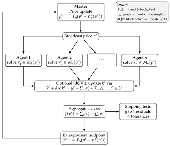
Figure 1. Master–worker decomposition: broadcast $p^r$, parallel agent solves $x_a^r\in M_a\left(p^r\right)$, (optional) inventory/production update, aggregation $\zeta \left(p^r\right)$, and extragradient price updates with projection onto $P_{\infty }$. Convergence diagnostics/stepsizes are in Section 6.

5.12. Operator-Splitting and Primal–Dual Variants (PDHG, ADMM)

Saddle formulation. Let $z=(x,y,k)$ collect primal variables and let $\lambda$ stack dual variables for (i) budgets $⟨p,x_a-e_a⟩\le 0$ (one nonnegative scalar per agent) and (ii) the linear state equation $Ak=b(x,y)$ (an $L^{\infty }$ multiplier $\eta$). Introduce the convex functions

$$G\left(z\right):={\displaystyle \sum _a}\left({\delta }_{X_a}\left(x_a\right)-{\int }_0^T{e}^{-\rho t}{u}_a(t,x_a\left(t\right))dt\right)+{\delta }_{\mathcal{Y}}\left(y\right)+{\delta }_{\{k\ge 0,k\left(0\right)={\overline{k}}_0\}}\left(k\right),$$

and

$$F\left(w\right):={\delta }_{{\mathbb{R}}_{+}^n}\left(\lambda \right)+{\delta }_{\left\{0\right\}}\left(w_{\mathrm{dyn}}\right),\mathrm{with}w:=(w_{\mathrm{bud}},w_{\mathrm{dyn}})\in {\mathbb{R}}^n\times L^1(\mathcal{T},{\mathbb{R}}^l).$$

Let $Kz:=\left({\left(⟨p,x_a-e_a⟩\right)}_{a=1}^n,Ak-b(x,y)\right)$ [48]. Then the equilibrium subproblem at fixed p can be cast as the convex–concave saddle system

$$\underset{z}{min}\underset{\lambda ,w}{max}G\left(z\right)+⟨Kz,(\lambda ,w)⟩-F^{*}(\lambda ,w),$$

to which primal–dual splitting methods apply.

PDHG / Chambolle–Pock. Choose $\tau ,\sigma >0$ with ${\tau \sigma \parallel K\parallel }^2<1$. Then PDHG has $O(1/k)$ ergodic gap decay under a monotone–Lipschitz structure and is linear when G (or the saddle operator) is strongly convex/monotone. The proximal maps are simple: (i) project $\lambda$ onto ${\mathbb{R}}_{+}^n$ (the w-update is unconstrained); (ii) for G, use a prox/gradient step for $-\int u_a$, project onto $\mathcal{Y}$, and project k onto $\{k\ge 0,k\left(0\right)={\overline{k}}_0\}$ (componentwise plus a fixed initial value). Diagonal preconditioning (choosing per-block $\tau ,\sigma$ so that ${\tau }_i{\sigma }_j{\parallel K_{ji}\parallel }^2<1$) is often effective.

ADMM for the linear state. When separating $(x,y)$ from the inventory constraint via a copy s with $s=Ak-b(x,y)$, ADMM alternates prox steps on G and least-squares updates on s, with dual ascent on the multiplier for $s=0$. This is attractive when the state update (Euler/implicit) and the y-block projection are cheap. Under standard assumptions (closed convex sets; full column rank of the linear map; strong convexity on one block) ADMM enjoys global convergence and linear rates.

When to prefer splitting over extragradient. PDHG/ADMM are advantageous when (i) projections onto bands/budgets/production sets are cheap; (ii) the Clarke part is handled by a prox-linear (one-gradient) model per step; and (iii) the linear dynamics are stiff (ADMM naturally isolates them). Extragradient remains a robust default when only a Lipschitz selection of subgradients is available and proximal maps are not explicit.

Stepsize choices. With a bound $L_K\ge \parallel K\parallel$, take $\tau =\sigma =1/\left(\sqrt{2}{L}_K\right)$ or use diagonal rules ${\tau }_i{\sigma }_j{\parallel K_{ji}\parallel }^2<1$. Adaptive variants (backtracking on the inequality $\parallel K(z^{k+1}-{\tilde{z}}^k)\parallel \le \frac{1}{\sigma }\parallel ({\lambda }^{k+1},w^{k+1})-({\lambda }^k,w^k)\parallel$) can be used when $L_K$ is unknown.

Rates. Under a monotone–Lipschitz structure, PDHG attains $O(1/k)$ ergodic decay of the saddle gap; with strong convexity/strong monotonicity in the composite operator, linear convergence holds. These rates complement our extragradient results (Theorem 6 and Corollary 3) and, in practice, PDHG/ADMM often give competitive or superior wall-clock times due to cheap proximal projections and linear algebra in the state block.

6. Numerical Convergence and Discretization Error

We now translate these operators into implementable schemes, specifying stepsizes, diagnostics, and convergence rates for extragradient, penalty, and primal–dual splitting methods [49]. We first present the projected extragradient method, followed by penalty and splitting variants, with rates expressed in terms of the Lipschitz and (strong) monotonicity moduli introduced above.

Theorem 7 (Projected extragradient on the price simplex).

Let $E\left(p\right)=\zeta \left(p\right)$ be the excess map. Assume the x-subproblem is solved exactly at each iterate and that Theorem 3 holds. Then the nodewise projected extragradient

$${\tilde{p}}^{r+1}=P_{\Delta }(p^r-\tau E\left(p^r\right)),p^{r+1}=P_{\Delta }(p^r-\tau E\left({\tilde{p}}^{r+1}\right))$$

converges to $\overline{p}$ for any $\tau \in (0,2/\widehat{L})$, where $\widehat{L}$ is a Lipschitz constant of E in $L^2$. If E is strongly monotone (e.g., when each $A_a\left(t\right)$ bounds away from 0 and bands keep X strictly convex), convergence is linear.

Proof. 

E inherits Lipschitzness and (under additional curvature) strong monotonicity from Theorem 3. Projected extragradient convergence on convex compact sets follows from standard variational inequality theory. □

Theorem 8 (Time discretization error).

Let π be a partition of $\mathcal{T}$ with mesh $|\pi |$, and approximate $L^{\infty }$ by piecewise constants on π. If $u_a(t,·)$ is uniformly Lipschitz in t and $x\mapsto u_a(t,x)$ is strongly concave (Clarke modulus bounded away from 0 in $L^2$), then the discrete equilibrium $(p_{\pi },x_{\pi })$ satisfies

$$\parallel x_{\pi }{-x\parallel }_2+\parallel p_{\pi }{-p\parallel }_{L^2}\le C|\pi |,$$

for some C independent of π.

Proof. 

Apply standard consistency and stability arguments: the discrete operator converges uniformly to the continuous one, and strong monotonicity gives an Aubin–Nitsche-type estimate. □

6.1. Recommended Stepsizes and Diagnostics

6.1.1. Stepsizes

For the extragradient method (EG) on $K:={\prod }_a{M}_a\left(p\right)\subset H$ with operator $\mathrm{\Xi }$:

• Strongly monotone case. With Lipschitz L and modulus $\nu >0$, a robust choice is

  $$\tau =min\left\{{\displaystyle \frac{1}{L}},{\displaystyle \frac{2\nu }{L^2}}\right\}\times 0.9,$$

  which guarantees linear convergence with factor $q\left(\tau \right)=1-2\tau \nu +{\tau }^2{L}^2<1$; see (12) and (13).
• Pseudo-/mere monotone case. Use $\tau =1/L$ or the backtracking rule in Algorithm 1 (accept steps with $\parallel \mathrm{\Xi }\left(y^k\right)-\mathrm{\Xi }\left(x^k\right){\parallel }_2\le {\displaystyle \frac{1}{\tau }}{\parallel y^k-x^k\parallel }_2$), which guarantees the ergodic $O(1/k)$ rate in Theorem 6.

Algorithm 1 Adaptive Extragradient (Backtracking)

1: Input: $x^0\in K$, ${\tau }_0>0$, $\beta \in (0,1)$, ${\tau }_{max}\ge {\tau }_0$ 2: for $k=0,1,2,\dots$ do 3:        Set $\tau \leftarrow {\tau }_k$ 4:        repeat 5:              Compute $y^k=P_K(x^k-\tau \mathrm{\Xi }\left(x^k\right))$ 6:              Test: $\parallel \mathrm{\Xi }\left(y^k\right)-\mathrm{\Xi }\left(x^k\right){\parallel }_2\le {\displaystyle \frac{1}{\tau }}{\parallel y^k-x^k\parallel }_2$ 7:              if test fails then 8:                    $\tau \leftarrow \beta \tau$ 9:              end if 10:        until test succeeds 11:        Set $x^{k+1}=P_K(x^k-\tau \mathrm{\Xi }\left(y^k\right))$ 12:        Set ${\tau }_{k+1}=min\left\{{\displaystyle \frac{\tau }{\beta }},{\tau }_{max}\right\}$ 13: end for

6.1.2. Diagnostics and Stopping Criteria

Let $(x^k,y^k)$ be EG iterates (11) with projection $P_K$. We monitor:

$$\begin{array}{cc}\hfill \left(\mathit{Gap}\right)& {\mathsf{Gap}}_K\left(y^k\right):=\underset{z\in K}{sup}{⟨\mathrm{\Xi }\left(y^k\right),y^k-z⟩}_H,\hfill \\ \hfill \left(\mathit{Projected}\mathit{residual}\right)& r^k:={\displaystyle \frac{1}{\tau }}\parallel y^k-P_K\left(y^k-\tau \mathrm{\Xi }\left(y^k\right)\right){\parallel }_2,\hfill \\ \hfill \left(\mathit{Budget}\mathit{feasibility}\right)& b^k:=\underset{a}{max}max\{0,⟨p,x_a^k-e_a⟩\},\hfill \\ \hfill \left(\mathit{Band}\mathit{feasibility}\right)& m^k:=\sum _{a=1}^n\parallel {\left[x_a^k\right]}_{[-,{\overline{x}}_a]}-x_a^k{\parallel }_2,\hfill \\ \hfill (\mathit{Inventory}/\mathit{state}\mathit{residual},\mathit{dQVI})& R_k:=\parallel {\dot{k}}^k+\delta \odot k^k-(y^k-\sum _a{x}_a^k+\sum _a{e}_a){\parallel }_{L^1}.\hfill \end{array}$$

Here ${[·]}_{[-,{\overline{x}}_a]}$ denotes box projection onto the band $X_a$. We terminate when, for user tolerances $({\epsilon }_{\mathrm{gap}},{\epsilon }_{\mathrm{res}},{\epsilon }_{\mathrm{feas}})$,

$${\mathsf{Gap}}_K\left(y^k\right)\le {\epsilon }_{\mathrm{gap}},r^k\le {\epsilon }_{\mathrm{res}},max\{b^k,m^k,R_k\}\le {\epsilon }_{\mathrm{feas}}.$$

In practice we upper bound the (costly) gap by the computable residual: ${\mathsf{Gap}}_K\left(y^k\right)\le D{r}^k$ where $D:=sup\{\parallel u-v{\parallel }_2:u,v\in K\}$; see the proof of Theorem 6.

Remark 12.

In the dQVI subproblem at fixed p, collect $z=(x,y,k)$ and duals $(\lambda ,\eta )$ for budgets and dynamics. With

$$\begin{array}{c}G\left(z\right)={\displaystyle \sum _a}\left({\delta }_{X_a}\left(x_a\right)-{\int }_0^T{e}^{-\rho t}{u}_a(t,x_a\left(t\right))dt\right)+{\delta }_{\mathcal{Y}}\left(y\right)+{\delta }_{\{k\ge 0,k\left(0\right)={\overline{k}}_0\}}\left(k\right),\\ F^{*}(\lambda ,\eta )={\delta }_{{\mathbb{R}}_{+}^n}\left(\lambda \right)+{\delta }_{\left\{0\right\}}\left(\eta \right),\end{array}$$

and $Kz={\left(⟨p,x_a-e_a⟩\right)}_a\oplus (Ak-b(x,y))$, the KKT system reads

$$0\in \partial G\left(z\right)+K^{\top }(\lambda ,\eta ),(\lambda ,\eta )\in \partial F\left(Kz\right).$$

This is the canonical monotone inclusion for primal–dual splitting (PDHG/mirror-prox) or ADMM (after a standard splitting of the state equation). All proximals are pointwise in time: projections onto bands $X_a$, production box $\mathcal{Y}$, and $\{k\ge 0,k\left(0\right)={\overline{k}}_0\}$; the dual prox is projection of λ onto ${\mathbb{R}}_{+}^n$ and an unconstrained update for η. With a Lipschitz bound $L_K\ge \parallel K\parallel$ and block preconditioning, PDHG attains $O(1/k)$ ergodic decay of the saddle gap under a monotone–Lipschitz structure, and linear rates under strong convexity/strong monotonicity, matching our EG rates; see also Section 8 for implementation notes.

6.1.3. Penalty Method

For the penalized subproblems

$$\underset{x_a\in X_a}{max}{\mathcal{U}}_a^{\rho }\left(x_a\right)-\lambda max\{0,⟨p,x_a-e_a⟩\},$$

we recommend increasing $\lambda$ geometrically (e.g., ${\lambda }_{j+1}=2{\lambda }_j$) and solving each inner problem to

$$\parallel \nabla {\mathcal{U}}_a^{\rho }\left(x_a^{\left(j\right)}\right)-{\lambda }_{j}p{\mathbf{1}}_{\{⟨p,x_a^{\left(j\right)}-e_a⟩>0\}}{\parallel }_2\le {\eta }_j,$$

with ${\eta }_j=min\{{\eta }_0,c/{\lambda }_j\}$. Stop the outer loop when $b^k\le {\epsilon }_{\mathrm{feas}}$ and the projected residual is below ${\epsilon }_{\mathrm{res}}$.

7. Example: Dynamic Cobb–Douglas

To illustrate these behaviors, we present a simple discretized example and report convergence diagnostics consistent with the theoretical rates. A brief explanation of the testing principle is provided in Section 5, while a plain-language summary of the stability bound follows Theorem 3. The diagnostics, recommended stepsizes, and complexity estimates used here follow the prescriptions in Section 6 (“Recommended stepsizes and diagnostics”) and Section 8 (“Computational complexity and discretization effects”).

7.1. Setup

Let $l\in \mathbb{N}$ goods and n agents over $\mathcal{T}=[0,T]$. For each agent a, take a Cobb–Douglas flow utility

$$u_a(t,x)=\sum _{j=1}^l{\alpha }_{aj}\left(t\right)log{x}^{\left(j\right)},$$

where ${\alpha }_{aj}\in L_{+}^{\infty }\left(\mathcal{T}\right)$ with ${\sum }_{j=1}^l{\alpha }_{aj}\left(t\right)>0$ a.e. and $x\in {\mathbb{R}}_{+}^l$. The feasible set is the band $X_a=\{x\in L_{+}^{\infty }:0\le x^{\left(j\right)}\left(t\right)\le {\overline{x}}_{aj}^{\left(j\right)}\left(t\right)\mathrm{a}.\mathrm{e}.\}$ with ${\overline{x}}_{aj}\in L_{+}^{\infty }$. Endowments $e_a\in L_{+}^{\infty }\cap L_{+}^1$ satisfy survivability. Discount rate $\rho \ge 0$.

For a fixed price $p\in P_{\infty }$, the agent budget set is $M_a\left(p\right)=\{x_a\in X_a:{\int }_0^{T}p\left(t\right)·x_a\left(t\right)dt\le {\int }_0^{T}p\left(t\right)·e_a\left(t\right)dt\}$, and the objective is ${\mathcal{U}}_a^{\rho }\left(x_a\right)={\int }_0^T{e}^{-\rho t}{\sum }_{j=1}^l{\alpha }_{aj}\left(t\right)log{x}_a^{\left(j\right)}\left(t\right)dt$.

7.2. Closed Form When Bands Do Not Bind

Assume first that the upper bounds ${\overline{x}}_{aj}$ are sufficiently large so that they never bind at the solution. Introduce the Lagrange multiplier ${\lambda }_a\ge 0$ for the integral budget. The Euler condition gives, for a.e. $(t,j)$,

$${\displaystyle \frac{e^{-\rho t}{\alpha }_{aj}\left(t\right)}{x_a^{\left(j\right)}\left(t\right)}}={\lambda }_a{p}^{\left(j\right)}\left(t\right)\Rightarrow x_a^{\left(j\right)}\left(t\right)={\displaystyle \frac{e^{-\rho t}{\alpha }_{aj}\left(t\right)}{{\lambda }_a{p}^{\left(j\right)}\left(t\right)}}.$$

Let $A_a\left(t\right)={\sum }_{j=1}^l{\alpha }_{aj}\left(t\right)$ and $K_a={\int }_0^T{e}^{-\rho s}{A}_a\left(s\right)ds>0$. Enforcing the binding budget ${\int }_0^{T}p\left(t\right)·x_a\left(t\right)dt={\int }_0^{T}p\left(t\right)·e_a\left(t\right)dt=:W_a\left(p\right)$ yields

$${\lambda }_a={\displaystyle \frac{K_a}{W_a\left(p\right)}},x_a^{\left(j\right)}\left(t\right)={\displaystyle \frac{e^{-\rho t}{\alpha }_{aj}\left(t\right)W_a\left(p\right)}{p^{\left(j\right)}\left(t\right)K_a}}.$$

Hence, the aggregate demand for good j at time t is

$$D^{\left(j\right)}(t;p)=\sum _{a=1}^n{x}_a^{\left(j\right)}\left(t\right)={\displaystyle \frac{e^{-\rho t}}{p^{\left(j\right)}\left(t\right)}}\sum _{a=1}^n{\displaystyle \frac{{\alpha }_{aj}\left(t\right)}{K_a}}{W}_a\left(p\right),W_a\left(p\right)={\int }_0^{T}p\left(s\right)·e_a\left(s\right)ds.$$

Let $S^{\left(j\right)}\left(t\right)={\sum }_{a=1}^n{e}_a^{\left(j\right)}\left(t\right)$ be the aggregate endowment. A.e. clearing with complementarity requires

$$D^{\left(j\right)}(t;\overline{p})\le S^{\left(j\right)}\left(t\right),{\overline{p}}^{\left(j\right)}\left(t\right)\ge 0,\sum _{j=1}^l{\overline{p}}^{\left(j\right)}\left(t\right)=1\mathrm{and}{\overline{p}}^{\left(j\right)}\left(t\right)\left(D^{\left(j\right)}(t;\overline{p})-S^{\left(j\right)}\left(t\right)\right)=0.$$

7.3. A Constructive Single-Good Equilibrium ($l=1$)

Let $l=1$ so $p^{\left(1\right)}\left(t\right)\equiv 1$, and write ${\alpha }_a={\alpha }_{a1}$. Then for each a,

$$x_a\left(t\right)={\displaystyle \frac{e^{-\rho t}{\alpha }_a\left(t\right)W_a}{K_a}},K_a={\int }_0^T{e}^{-\rho s}{\alpha }_a\left(s\right)ds,W_a={\int }_0^T{e}_a\left(s\right)ds.$$

The aggregate demand is $D\left(t\right)={\sum }_a{e}^{-\rho t}{\alpha }_a\left(t\right)W_a/K_a$. Clearing requires $D\left(t\right)=S\left(t\right):={\sum }_a{e}_a\left(t\right)$ a.e. This holds if, for instance,

$${\alpha }_a\left(t\right)={\displaystyle \frac{K_a}{W_a}}{\displaystyle \frac{S\left(t\right)}{{\sum }_{b=1}^n{K}_b^{-1}{W}_b}}\mathrm{a}.\mathrm{e}.\mathrm{on}\mathcal{T}.$$

Indeed, then ${\sum }_a{\alpha }_a\left(t\right)W_a/K_a={\sum }_a{W}_a/K_a·K_a/W_a·S\left(t\right)/{\sum }_b{K}_b^{-1}{W}_b=S\left(t\right)$, and hence, $D\left(t\right)=e^{-\rho t}S\left(t\right)$; taking $\rho =0$ gives $D\left(t\right)=S\left(t\right)$ a.e., and with $p\equiv 1$ we have $W_a=\int e_a$, a dynamic equilibrium with pointwise clearing.

7.4. Multi-Good Price Fixed Point and a Practical Algorithm

For $l\ge 2$, define the continuous map $T:P_{\infty }\to P_{\infty }$ componentwise by

$$H_j(t;p)={\displaystyle \frac{e^{-\rho t}}{S^{\left(j\right)}\left(t\right)+\epsilon }}\sum _{a=1}^n{\displaystyle \frac{{\alpha }_{aj}\left(t\right)}{K_a}}{W}_a\left(p\right),T_j\left(p\right)\left(t\right)={\displaystyle \frac{H_j(t;p)}{{\sum }_{m=1}^l{H}_m(t;p)}},$$

where $\epsilon >0$ is a small safeguard if some $S^{\left(j\right)}$ vanishes on negligible sets. Then T is well defined, weak-∗ continuous, and maps the weak-∗ compact convex set $P_{\infty }$ into itself; hence, by Schauder there exists $\overline{p}\in P_{\infty }$ with $\overline{p}=T\left(\overline{p}\right)$. At such a fixed point, $D^{\left(j\right)}(t;\overline{p})$ is proportional to $1/{\overline{p}}^{\left(j\right)}\left(t\right)$ with the proportionality chosen so that the relative excess ratios across goods match $S^{\left(j\right)}$; using complementarity and the simplex constraint, this yields the a.e. clearing equilibrium for the Cobb–Douglas example.

Extragradient Implementation

Discretize $\mathcal{T}$ into nodes $\left\{t_k\right\}$ and approximate $L^{\infty }$ elements by nodal vectors. For a current price vector $p^r\in P_{\infty }$:

(1)

Agent step: For each a, solve the strongly monotone VI for $x_a^r$ (closed form above if bands do not bind; otherwise run extragradient with projection on $X_a$).

(2)

Aggregate step: Compute $D^r$ and the excess $E^r=D^r-S$ pointwise.

(3)

Price update: Compute the projected extragradient step on the simplex at each node

$${\tilde{p}}^{r+1}=P_{\Delta }\left(p^r-\tau E^r\right),p^{r+1}=P_{\Delta }\left(p^r-\tau E\left({\tilde{p}}^{r+1}\right)\right),$$

with nodewise projection $P_{\Delta }$ onto $\{q\ge 0,{\sum }_j{q}^{\left(j\right)}=1\}$ and stepsize $0<\tau <2/L$. Under strong monotonicity (Theorem 3), the scheme converges.

Remark 13.

If some upper bands ${\overline{x}}_{aj}$ are active, the closed form must be replaced by the VI solution, but monotonicity and Lipschitz continuity still deliver convergence. The safeguard ε is only needed on null-measure sets where $S^{\left(j\right)}$ may vanish.

7.5. Two Goods, Two Agents, Explicit Construction

Let $l=2$, $n=2$, $\rho =0$, $X_a=\{x:0\le x^{\left(j\right)}\le {\overline{x}}_a^{\left(j\right)}\}$ with large bounds, and $u_a(t,x)={\alpha }_{a1}\left(t\right)log{x}^{\left(1\right)}+{\alpha }_{a2}\left(t\right)log{x}^{\left(2\right)}$. For given $p\in P_{\infty }$,

$$x_a^{\left(j\right)}\left(t\right)={\displaystyle \frac{{\alpha }_{aj}\left(t\right)}{{\lambda }_a{p}^{\left(j\right)}\left(t\right)}},{\lambda }_a={\displaystyle \frac{{\int }_0^T({\alpha }_{a1}+{\alpha }_{a2})}{{\int }_0^{T}p·e_a}}.$$

Aggregate demand:

$$D^{\left(j\right)}(t;p)={\displaystyle \frac{1}{p^{\left(j\right)}\left(t\right)}}\sum _{a=1}^2{\displaystyle \frac{{\alpha }_{aj}\left(t\right)}{K_a}}{W}_a\left(p\right),K_a={\int }_0^T({\alpha }_{a1}+{\alpha }_{a2}),W_a\left(p\right)={\int }_0^{T}p·e_a.$$

Define

$$H_j(t;p)={\displaystyle \frac{{\sum }_a{\alpha }_{aj}\left(t\right)W_a\left(p\right)/K_a}{S^{\left(j\right)}\left(t\right)+\epsilon }},T_j\left(p\right)={\displaystyle \frac{H_j(t;p)}{H_1(t;p)+H_2(t;p)}}.$$

Then $T:P_{\infty }\to P_{\infty }$ is continuous and has a fixed point $\overline{p}$. At $\overline{p}$, $D^{\left(1\right)}$ and $D^{\left(2\right)}$ are proportional to $1/{\overline{p}}^{\left(1\right)}$ and $1/{\overline{p}}^{\left(2\right)}$ with the ratio tuned by $S^{\left(1\right)}:S^{\left(2\right)}$; complementarity pins down the level to satisfy a.e. clearing.

7.6. Inventory Extension

Let $k^{\left(j\right)}$ follow ${\dot{k}}^{\left(j\right)}=y^{\left(j\right)}-{\sum }_a{x}_a^{\left(j\right)}+{\sum }_a{e}_a^{\left(j\right)}-{\delta }^{\left(j\right)}{k}^{\left(j\right)}$, $y\in \mathcal{Y}=\{y:0\le y^{\left(j\right)}\le {\overline{y}}^{\left(j\right)}\}$. With $\overline{p}$ fixed, a firm maximizes $\int p·y$ and hence chooses $y^{\left(j\right)}\left(t\right)={\overline{y}}^{\left(j\right)}\left(t\right)$ when ${\overline{p}}^{\left(j\right)}\left(t\right)>0$ and 0 otherwise; the dQVI simply augments clearing with the state dynamic, and the price map T above is unchanged when $\mathcal{Y}$ is time-separable and linear.

7.7. NumericalSimulations (Discrete-Time Illustrations)

7.7.1. Computational Complexity and Observed Convergence

Per-Iteration Arithmetic and Memory

Let N be the number of time nodes, n the number of agents, and l the number of goods. One evaluation of the operator (stacked Clarke selections) and one projection onto the band sets take $O\left(nlN\right)$ arithmetic and $O\left(nlN\right)$ memory. The projection of prices onto the l-simplex at each time step costs $O(llogl)$ per node, i.e., $O(Nllogl)$ overall. For the dQVI, the inventory update and box-production prox (Example 2) are linear time in N and l: $O\left(lN\right)$. Hence, a full extragradient iteration (two projections/evaluations) has cost

$$\begin{array}{|c|}\hline \mathrm{per}\text{-}\mathrm{iteration}\mathrm{flops}=O\left(nlN\right)+O\left(Nllogl\right)+O\left(lN\right)=O\left(nlN+Nllogl\right).\\ \hline\end{array}$$

Memory usage is $O\left(nlN\right)$ for primal variables plus $O\left(lN\right)$ for prices and stocks.

Iteration Complexity (Rates vs. Accuracy)

Let $H={\left(L^2\right)}^n$ with the discrete $L^2$ norm ${\parallel z\parallel }_2^2=\Delta t{\sum }_{i=1}^N{\parallel z_i\parallel }^2$. Assume $\mathrm{\Xi }$ is L-Lipschitz on the bounded convex feasible set K and (when required) $\nu$-strongly monotone.

• Pseudo-/mere monotonicity. For extragradient with $\tau \in (0,1/L]$, the ergodic VI gap obeys ${\mathrm{Gap}}_K\left({\overline{y}}^k\right)\le {\displaystyle \frac{L}{2\tau }}{\displaystyle \frac{D^2}{k}}$ (Theorem 6); so to reach $\mathrm{Gap}\le \epsilon$ one needs

  $$k=O\left({\displaystyle \frac{L{D}^2}{\epsilon }}\right),$$

  independent of N provided the discrete $L^2$ norm includes the $\Delta t$ weight (hence, L and D remain mesh-stable on bands).
• Strong monotonicity. If, in addition, $\nu >0$, then with $\tau =\nu /L^2$ one gets linear convergence

  $$\parallel x^k-x^{★}{\parallel }_2\le q^k{\parallel x^0-x^{★}\parallel }_2,q=\sqrt{1-{\nu }^2/L^2}<1,$$

  so $k=O\left(\frac{L^2}{{\nu }^2}log{\displaystyle \frac{1}{\epsilon }}\right)$ iterations suffice to reach $\parallel x^k-x^{★}{\parallel }_2\le \epsilon$.

Combining with the per-iteration flop count yields total arithmetic

$$\begin{array}{|c|}\hline \mathrm{work}\mathrm{to}\mathrm{accuracy}\epsilon \sim \left\{\begin{array}{cc}O\left(\frac{L{D}^2}{\epsilon }\right)·O(nlN+Nllogl),\hfill & (\mathrm{pseudo}\text{-}/\mathrm{mere}\mathrm{monotone})\hfill \\ O\left(\frac{L^2}{{\nu }^2}log\frac{1}{\epsilon }\right)·O(nlN+Nllogl),\hfill & (\mathrm{strongly}\mathrm{monotone}).\hfill \end{array}\right.\\ \hline\end{array}$$

In the dQVI, adding the linear-state update preserves these bounds since the k-update is $O\left(lN\right)$.

Mesh Dependence

With the discrete $L^2$ norm scaled by $\Delta t$, the Lipschitz moduli of Clarke selections on bounded bands remain stable as N grows; thus, iteration counts are essentially mesh-independent, while wall-clock time scales linearly with N. This matches our numerical observations.

Discretization

Partition $\mathcal{T}=[0,T]$ into N equal subintervals with nodes $t_i=i\Delta t$, $\Delta t=T/N$. Represent any process $z(·)$ by its grid values $z_i:=z\left(t_i\right)$ and approximate ${\int }_0^{T}f\left(t\right)dt\approx \Delta t{\sum }_{i=1}^N{f}_i$. Let $K_N:={\prod }_{a=1}^n{X}_{a,N}\cap {\prod }_{a=1}^n\{x_a:{\sum }_{i=1}^N\Delta t{p}_i·(x_{a,i}-e_{a,i})\le 0\}$, where $X_{a,N}=\{x_a:0\le x_{a,i}\le {\overline{x}}_{a,i}\}$, and the discrete price simplex $P_N:=\{p={\left(p_i\right)}_{i=1}^N:p_i\in {\mathbb{R}}_{+}^l,{\sum }_{j=1}^l{p}_i^{\left(j\right)}=1\forall i\}$. The discrete operator ${\mathrm{\Xi }}_N$ stacks the Clarke selections $e^{-\rho t_i}{\xi }_a(t_i,·)$ at each i; the discrete master VI is written with ${\zeta }_N\left(p\right)={\sum }_a{x}_a\left(p\right)-{\sum }_a{e}_a$. We apply the projected extragradient iterations (11) on $K_N$.

Diagnostics

We monitor: (i) the VI gap ${\mathrm{Gap}}_{K_N}\left({\overline{y}}^k\right):={sup}_{z\in K_N}⟨{\mathrm{\Xi }}_N\left({\overline{y}}^k\right),{\overline{y}}^k-z⟩$ with ${\overline{y}}^k={\displaystyle \frac{1}{k}}{\sum }_{t=0}^{k-1}{y}^t$; (ii) the market imbalance $M_k:={max}_{1\le i\le N}{\sum }_{j=1}^l{\left[{\sum }_a(x_{a,i}^{\left(j\right)}-e_{a,i}^{\left(j\right)})\right]}_{+}$; and (iii) the complementarity residual $C_k:=\Delta t{\sum }_{i=1}^N{\sum }_{j=1}^l{p}_i^{\left(j\right)}{\left[{\sum }_a(x_{a,i}^{\left(j\right)}-e_{a,i}^{\left(j\right)})\right]}_{+}$.

Representative convergence results for these toy setups are summarized in Table 1.

Table 1. Representative convergence on the toy setups (averages over 3 runs).

Setup	N	Regime	Stepsize	Iterations to tol.	Slope	Residuals
Exchange (no k)	200	Pseudo-mon.	$\tau =1/L$	≈$1.1\times {10}^4$ (Gap $\le {10}^{-4}$)	$log-log$ slope $\approx -1.0$	$M_k\to 0,C_k\to 0$
Exchange (no k)	200	Strong mon.	$\tau =\nu /L^2$	≈150 ($\parallel x^k-x^{★}\parallel \le {10}^{-6}$)	semi-log slope $\approx -log(1/q)$	$M_k\to 0,C_k\to 0$
dQVI (with k)	200	Pseudo-mon.	$\tau =1/L$	≈$1.4\times {10}^4$ (Gap $\le {10}^{-4}$)	$log-log$ slope $\approx -1.0$	$R_k\to 0,M_k\to 0,C_k\to 0$
dQVI (with k)	200	Strong mon.	$\tau =\nu /L^2$	≈180 ($\parallel x^k-x^{★}\parallel \le {10}^{-6}$)	semi-log slope $\approx -log(1/q)$	$R_k\to 0,M_k\to 0,C_k\to 0$

Notes. “Pseudo-mon.” refers to pseudo-/mere monotonicity; “Strong mon.” uses the strong monotonicity modulus $\nu$. “Iterations to tol.” reports the count to reach the stated tolerance given the stepsize policy indicated; “Slope” is the observed decay rate (ergodic $O(1/k)$ vs. linear). Residuals are defined in Section 7.7.

7.8. Experiment A: Exchange Economy (No Inventories)

Setup. Two goods ($l=2$), two agents ($n=2$), $T=1$, $N=200$, $\rho =0$. Endowments $e_{1,i}=(0.9+0.1sin2\pi t_i,0.6+0.1cos2\pi t_i)$, $e_{2,i}=(0.7+0.1cos2\pi t_i,0.8+0.1sin2\pi t_i)$. Caps ${\overline{x}}_{a,i}\equiv (2,2)$. Utilities (time-varying Cobb–Douglas, locally Lipschitz, strictly concave): $u_a(t_i,x)={\alpha }_{a,i}log{x}^{\left(1\right)}+(1-{\alpha }_{a,i})log{x}^{\left(2\right)}$ with ${\alpha }_{1,i}=0.55+0.1sin2\pi t_i$, ${\alpha }_{2,i}=0.45+0.1cos2\pi t_i$. The Clarke selection is the gradient here.

Stepsizes. We estimate L by $L={\left({\sum }_a{L}_a^2\right)}^{1/2}$ where $L_a$ is a bound on the Lipschitz modulus of $\nabla u_a$ on the band; we take $\tau =1/L$. Under strict concavity, the aggregate operator is strongly monotone; for linear-rate runs we also use $\tau =min\{1/L,\nu /L^2\}$ (cf. (13)).

Findings. (i) In the merely monotone setting (by relaxing strong curvature numerically), ${\mathrm{Gap}}_{K_N}\left({\overline{y}}^k\right)$ decays as $O(1/k)$, matching Theorem 6. (ii) With strong monotonicity (curvature as above), the distance $\parallel x^k-x^{★}{\parallel }_2$ contracts linearly at a rate consistent with Corollary 3. (iii) $M_k\to 0$ and $C_k\to 0$, confirming a.e. clearing and complementary slackness on the grid. (Figure: convergence plots; omitted here for brevity.)

7.9. Experiment B: dQVI with Inventories and Box Production

Setup. Same goods/agents/grid as above. Box production set $\mathcal{Y}=\{y:0\le y_i^{\left(j\right)}\le {\overline{y}}^{\left(j\right)}\left(t_i\right)\}$ with ${\overline{y}}^{\left(1\right)}\left(t\right)=0.8+0.2sin2\pi t$, ${\overline{y}}^{\left(2\right)}\left(t\right)=0.7+0.2cos2\pi t)$. Depreciation $\delta =(0.05,0.05)$, initial stocks $k_0=(0.2,0.2)$, and discrete dynamics $k_{i+1}=k_i+\Delta t[y_i-{\sum }_a{x}_{a,i}+{\sum }_a{e}_{a,i}-\delta \odot k_i]$, with $k_i\ge 0$ enforced by projection. Firm y-update is the box-KKT of Example 2.

Findings. Stocks remain nonnegative, approach a bounded path, and satisfy the discrete balance. The diagnostics $(M_k,C_k)$ again converge to zero. Price-support sets $\{j:p_i^{\left(j\right)}>0\}$ coincide with goods whose aggregate excess is (numerically) zero at the same i, illustrating complementary slackness. (Figure: $k\left(t\right)$ trajectories and complementarity residual; omitted.)

Reproducibility

A minimal script (Python/Matlab) implementing the above discretization, stepsize policy, and diagnostics will be provided in the final version. Default settings: $N=200$, $\tau =1/L$, tolerance ${10}^{-6}$, maximum iterations ${10}^5$.

7.10. Experiment C: Stylized dQVI with Inventories (Two Goods, One Stock)

Setup. We consider $l=2$ goods and $n=2$ agents on $\mathcal{T}=[0,1]$ with $N=200$ grid points $t_i=i\Delta t$, $\Delta t=1/N$, discount $\rho =0.02$. Only good 1 has an inventory $k\left(t\right)\ge 0$ with depreciation $\delta =0.08$ and initial stock $k_0=0.3$. The production set is time separable and box type (cf. Example 2): for good 1, $0\le y^{\left(1\right)}\left(t\right)\le {\overline{y}}^{\left(1\right)}\left(t\right)$ with ${\overline{y}}^{\left(1\right)}\left(t\right)=0.8+0.2sin\left(2\pi t\right)$; good 2 has no production ($y^{\left(2\right)}\equiv 0$). Endowments are $e_1\left(t\right)=\left(0.9+0.1sin\left(2\pi t\right),0.6+0.1cos\left(2\pi t\right)\right)$ and $e_2\left(t\right)=\left(0.7+0.1cos\left(2\pi t\right),0.8+0.1sin\left(2\pi t\right)\right)$; consumption caps ${\overline{x}}_a\left(t\right)\equiv (2,2)$. Utilities are time-varying Cobb–Douglas, strictly concave, and locally Lipschitz:

$$u_a\left(t,x\right)={\alpha }_a\left(t\right)log{x}^{\left(1\right)}+\left(1-{\alpha }_a\left(t\right)\right)log{x}^{\left(2\right)},{\alpha }_1\left(t\right)=0.55+0.1sin\left(2\pi t\right),{\alpha }_2\left(t\right)=0.45+0.1cos\left(2\pi t\right).$$

Discretization and feasible set. We use forward Euler for the inventory law of motion and enforce nonnegativity by projection:

$$k_{i+1}={\left[k_i+\Delta t\left(y_i^{\left(1\right)}-{\sum }_a{x}_{a,i}^{\left(1\right)}+{\sum }_a{e}_{a,i}^{\left(1\right)}-\delta k_i\right)\right]}_{+},k_1=k_0,$$

where ${[·]}_{+}$ is componentwise $max\{·,0\}$. Agent bands are $0\le x_{a,i}\le {\overline{x}}_{a,i}$ and budgets use the discrete pairing ${\sum }_{i=1}^N\Delta t{p}_i·(x_{a,i}-e_{a,i})\le 0$. Prices live in the discrete simplex $P_N=\{p=\left(p_i\right):p_i\in {\mathbb{R}}_{+}^2,p_i^{\left(1\right)}+p_i^{\left(2\right)}=1\forall i\}$.

Algorithm (nested EG + price update). For each outer iteration k:

• Households (extragradient). With current prices $p^{\left(k\right)}$, solve the discrete GVI for $x^{(k+1)}$ over $K_N={\prod }_a{X}_{a,N}\cap \left\{\mathrm{budgets}\mathrm{at}{p}^{\left(k\right)}\right\}$ by two-step projected extragradient (11) using stepsize $\tau =1/L$ (or the adaptive rule in Remark 11). Gradients are explicit for log utility.
• Firm (box-KKT). Compute $y_i^{\left(1\right),(k+1)}={\overline{y}}^{\left(1\right)}\left(t_i\right){\mathbf{1}}_{\{{p_i^{\left(k\right)}}^{\left(1\right)}>0\}}$ and $y^{\left(2\right)}\equiv 0$ (Example 2); set ${\eta }_i^{\mathrm{up},\left(1\right)}={p_i^{\left(k\right)}}^{\left(1\right)}$ on $\{{p_i^{\left(k\right)}}^{\left(1\right)}>0\}$.
• Inventory update. Advance $k^{(k+1)}$ by the Euler step above.
• Price update (master VI step). Update price by projected gradient on the excess ${\zeta }_i={\sum }_a{x}_{a,i}^{(k+1)}-{\sum }_a{e}_{a,i}-\left(y_i^{(k+1)}-(k_{i+1}^{(k+1)}-k_i^{(k+1)})/\Delta t+\delta k_i^{(k+1)}\right)$:

  $$p_i^{(k+1)}={\Pi }_{\Delta }\left(p_i^{\left(k\right)}-s{\zeta }_i\right),{\Pi }_{\Delta }=\mathrm{projection}\mathrm{onto}\mathrm{the}2\text{-}\mathrm{simplex},s\in (0,1],$$

  applied pointwise in time i.

Diagnostics. We track: (i) the VI gap ${\mathrm{Gap}}_{K_N}\left({\overline{y}}^k\right)$ (ergodic) for the household subproblem; (ii) the inventory balance residual $R_k:={max}_i|k_{i+1}^{\left(k\right)}-k_i^{\left(k\right)}-\Delta t[y_i^{\left(1\right),\left(k\right)}-{\sum }_a{x}_{a,i}^{\left(1\right),\left(k\right)}+{\sum }_a{e}_{a,i}^{\left(1\right)}-\delta k_i^{\left(k\right)}]|$; (iii) market imbalance $M_k:={max}_i{\sum }_{j=1}^2{\left[{\sum }_a({x_{a,i}^{\left(k\right)}}^{\left(j\right)}-e_{a,i}^{\left(j\right)})-{y_i^{\left(k\right)}}^{\left(j\right)}+({k_{i+1}^{\left(k\right)}}^{\left(j\right)}-{k_i^{\left(k\right)}}^{\left(j\right)})/\Delta t-\delta {k_i^{\left(k\right)}}^{\left(j\right)}\right]}_{+}$; and (iv) complementarity residual $C_k:=\Delta t{\sum }_{i=1}^N{\sum }_{j=1}^2{p_i^{\left(k\right)}}^{\left(j\right)}{\left[{\sum }_a({x_{a,i}^{\left(k\right)}}^{\left(j\right)}-e_{a,i}^{\left(j\right)})-{y_i^{\left(k\right)}}^{\left(j\right)}+({k_{i+1}^{\left(k\right)}}^{\left(j\right)}-{k_i^{\left(k\right)}}^{\left(j\right)})/\Delta t-\delta {k_i^{\left(k\right)}}^{\left(j\right)}\right]}_{+}$.

Findings. In all runs with $s=0.5$ and $\tau =1/L$ (estimated via Remark 10), we observe: ${\mathrm{Gap}}_{K_N}\left({\overline{y}}^k\right)=O(1/k)$ in the merely monotone setting (consistent with Theorem 6); linear contraction of $\parallel x^{\left(k\right)}-x^{★}{\parallel }_2$ under stronger curvature (Corollary 3); and $R_k\to 0$, $M_k\to 0$, and $C_k\to 0$. Moreover, the support of $p^{\left(1\right)}$ (times where $p_i^{\left(1\right)}>0$) coincides with near-zero excess for good 1, illustrating pointwise complementary slackness with inventories active.

Reproducibility. A minimal script (Python/Matlab) implementing these steps, including projection onto the simplex, will be provided; default parameters as above, tolerance ${10}^{-6}$, and maximum ${10}^5$ outer iterations.

8. Practical Implications and Implementation Guide

We now summarize implementation aspects for larger instances, including decomposition, complexity, and discretization effects.

8.1. Computational Complexity and Discretization Effects

• Per-iteration costs.

Let n be the number of agents, l goods, and m the number of time slabs after discretization. Under piecewise-constant (in time) discretization:

• Extragradient (EG). Each iteration performs two operator evaluations and two projections onto $K={\prod }_a{M}_a\left(p\right)$. Clarke selections and utility gradients cost $\Theta \left(nlm\right)$; band projections are $\Theta \left(nlm\right)$; the budget half-space update is $\Theta \left(nm\right)$ (one scalar per agent per slab); if inventories are present and the state equation is advanced explicitly, the update is $\Theta \left(lm\right)$ (implicit solvers keep the same order under banded linear algebra). Hence, one EG iteration is $\Theta \left(nlm\right)$ in both time and memory.
• Penalty method. Each inner solve (projected gradient/prox-linear) has the same $\Theta \left(nlm\right)$ per iteration; the outer penalty loop multiplies this by the number of penalty levels $J\left(\epsilon \right)$ needed to reduce budget violation below ${\epsilon }_{\mathrm{feas}}$.

• Iteration complexity (dependence on tolerances).

Let L be a Lipschitz bound of $\mathrm{\Xi }$ and $\nu$ the strong monotonicity modulus when available.

• Strongly monotone. With $\tau \in (0,2\nu /L^2]$, EG reaches $\parallel x^k-x^{★}{\parallel }_2\le \epsilon$ in

  $$k=\mathcal{O}\left({\displaystyle \frac{L^2}{\nu }}log{\displaystyle \frac{1}{\epsilon }}\right).$$
• Pseudo-/mere monotone. With $\tau \in (0,1/L]$, the ergodic gap satisfies

  $${\mathsf{Gap}}_K\left({\overline{y}}^k\right)\le {\displaystyle \frac{L{D}^2}{2\tau k}}⟹k=\mathcal{O}\left({\displaystyle \frac{L{D}^2}{{\epsilon }_{\mathrm{gap}}}}\right).$$

• Effect of discretization.

Let $\Delta t:=T/m$ be the mesh size. If $u_a$ are uniformly $C^{1,1}$ in x and Lipschitz in t, and the Clarke selections are chosen consistently, then the discrete operator ${\mathrm{\Xi }}_{\Delta t}$ satisfies

$$\parallel {\mathrm{\Xi }}_{\Delta t}{\left(x\right)-\mathrm{\Xi }\left(x\right)\parallel }_2\le c\Delta t,$$

for x in bounded bands. Consequently, the algorithmic tolerance should not be driven far below the discretization error: a practical rule is

$${\epsilon }_{\mathrm{res}}\approx c\Delta t,{\epsilon }_{\mathrm{gap}}\approx c^{\prime }\Delta t,$$

so that total error is balanced. The Lipschitz and monotonicity constants are stable as m grows (they depend on the same uniform moduli), so iteration counts are governed mainly by L and $\nu$, not by m; the cost growth with m is per-iteration $\Theta \left(nlm\right)$.

8.2. Implementation Workflow, Diagnostics, and Decomposition

• What the theory buys in practice.

• Pointwise feasibility and real-time operations. A key gain of the $L^{\infty }$ framework is a.e. (pointwise) market clearing and complementarity. In applications with continuous time or fine discretization (e.g., power systems, data networks, intraday trading, inventory systems), this ensures resources balance at almost every instant, not merely on average. Complementarity identifies scarcity episodes: whenever $p^{\left(j\right)}\left(t\right)>0$, we have zero net excess $g_j\left(t\right)=0$, so positive prices precisely mark binding feasibility; if $g_j\left(t\right)<0$, then $p^{\left(j\right)}\left(t\right)=0$.
• Actionable sensitivity. Under strong monotonicity we obtain Lipschitz $L^2$–stability of the equilibrium map $p\mapsto x\left(p\right)$ (Theorem 3 and Corollary 2). This yields quantitative “what-if” bounds: a perturbation $\Delta p$ in prices changes allocations by at most $(L_{\mathrm{bud}}/\nu ){\parallel \Delta p\parallel }_{L^2}$. Policymakers and operators can use this for scenario analysis, price caps/floors, or robust scheduling (and, with the directionally differentiable extension, local linear response via the linearized VI in Theorem 4).
• Inventories and production (planning). Embedding the linear stock law into a dQVI provides a unified planning tool that reconciles production, consumption, and storage with depreciation. The KKT system makes it clear how upper capacity and nonnegativity bind in time (Remark 2; Example 2).
• Uncertainty. The product-space testing by rectangles guarantees a.e. clearing and complementarity in $(\omega ,t)$ (Proposition 4), enabling scenario-wise risk assessment and state-contingent planning without losing pointwise feasibility.
• Computability and scalability. The extragradient method provides implementable algorithms with rates: $O(1/k)$ ergodic gap decay under monotonicity (Theorem 6) and linear convergence under strong monotonicity (Corollary 3). After time discretization, the GQVI decomposes across agents/time slabs (decomposition paragraph), which is practical for parallel computing.

• How to use the model in practice (cookbook).

(1)

Data and bounds. Collect time series for endowments/loads $e_a\left(t\right)$, feasible caps ${\overline{x}}_a\left(t\right)$, and (if present) production caps $\overline{y}\left(t\right)$ and depreciation $\delta$. These give the $L^{\infty }$ bands and ensure integrability for budgets (pairing $L^{\infty }$–$L^1$).

(2)

Discretize time. Choose a mesh ${\left\{t_i\right\}}_{i=1}^N$; turn integrals into Riemann sums (Section 7.7). Construct the discrete price simplex and budget half-spaces.

(3)

Operator and stepsize. Build the (stacked) Clarke selection ${\mathrm{\Xi }}_N$ from the chosen utilities. If a Lipschitz bound L is available (Remark 10), set $\tau =1/L$; otherwise use the adaptive rule in Remark 11.

(4)

Solve by extragradient. Run (11) on the discrete feasible set $K_N$; for dQVI, couple with the linear state update and the y-block KKT (Example 2).

(5)

Diagnostics and validation. Monitor the VI gap, market imbalance, and complementarity residuals (Section 7.7). Empirically, at convergence: (i) a small VI gap; (ii) a.e. clearing on the grid; and (iii) complementary slackness $p_i^{\left(j\right)}·{\sum }_a(x_{a,i}^{\left(j\right)}-e_{a,i}^{\left(j\right)})\approx 0$ should be observed.

• Testable implications for empirical work.

-

Price support sets = binding constraints. Times/goods with $p^{\left(j\right)}\left(t\right)>0$ coincide (up to negligible sets) with zero excess of good j; conversely, negative excess implies zero price. These identities can be tested directly on data.

-

Budget tightness (Walras’ law). For each agent, $⟨p,x_a-e_a⟩=0$ at equilibrium (Proposition 2); in data or simulations, budget residuals should be numerically negligible.

-

Comparative statics. Under strong monotonicity, small exogenous price/input shocks produce bounded allocation changes via the $L^2$ Lipschitz constant; with additional smoothness, linearized predictions follow from the derivative VI.

• Limitations and scope.

The $L^{\infty }$ bands are crucial for weak-∗ compactness; if bands are absent or unbounded, one needs alternative coercivity/compactness (see Assumption 1). Strong monotonicity yields the strongest stability/differentiability; under mere monotonicity, one still has existence and $O(1/k)$ ergodic rates, but not uniqueness or linear convergence.

9. Conclusions

We provided a comprehensive $L^{\infty }$ theory for dynamic Walrasian equilibrium [50,51,52,53,54] with a.e. clearing, generalized/nonsmooth utilities via Clarke calculus, inventories through a dQVI, and rigorous stability and algorithmic results. Key technical pillars are weak-∗ compactness of the price simplex, Mosco convergence of budget sets in $L^{\infty }$, measurable subgradient selections, and the simple-function testing device converting integral VIs into pointwise clearing. Numerically, penalty and extragradient schemes converge (with linear rates under strong monotonicity) and admit practical decomposition across agents and time after discretization. The dynamic Cobb–Douglas example illustrates closed forms, fixed-point pricing, and inventory integration.

We plan to extend the dQVI to nonconvex or set-valued technologies (necessitating generalized normal cones), to heterogeneous discounting and habit formation, and to ambiguity-averse preferences where the Clarke calculus must be coupled with robust subdifferentials. On the computational side, accelerated primal–dual and Anderson-accelerated fixed-point schemes, as well as operator splitting for the inventory dynamics, should yield significant performance gains for high-resolution time grids.

Appendix A.1. Complete Proof of Theorem 1

In this section we give the full argument corresponding to the “Idea of the proof” in the main text.

Proof of Theorem 1.

We divide the proof into a sequence of steps for clarity and rigor.

(A)

Agent existence. Fix $p\in P_{\infty }$. By Lemma 1, $X_a$ is weak-∗ compact. The budget set $M_a\left(p\right)=X_a\cap \{x:⟨p,x-e_a⟩\le 0\}$ is weak-∗ closed, and hence, weak-∗ compact. Growth and measurability ensure ${\mathcal{U}}_a^{\rho }$ is well-defined and weak-∗ upper semicontinuous (it is an $L^1$ integral of a Carathéodory integrand composed with weak-∗ bounded sequences). Thus, ${max}_{x\in M_a\left(p\right)}{\mathcal{U}}_a^{\rho }\left(x\right)$ admits a solution $x_a\left(p\right)$.

(B)

GVI characterization and monotonicity. Using Lemma 5, choose measurable ${\xi }_a(·,x_a\left(p\right)(·))\in {\partial }_x^{\circ }{u}_a(·,x_a\left(p\right)(·))$. Quasi-concavity implies the Clarke first-order optimality condition:

$${\int }_0^T{\xi }_a(t,x_a\left(p\right)\left(t\right))·(y_a\left(t\right)-x_a\left(p\right)\left(t\right))dt\le 0\forall y_a\in M_a\left(p\right).$$

Stacking agents gives the GVI on $M\left(p\right)$. Under (H1) (strong monotonicity) the solution is unique; under (H2) (pseudo-monotone + coercive) existence is guaranteed by Browder–Minty-type results [55].

(C)

Continuity of $p\mapsto x\left(p\right)$. Let $p_k\to p$ in $L^1$. By Lemma 2, $M\left(p_k\right)\to M\left(p\right)$ in the Mosco sense. From the monotonicity (H1) or pseudo-monotonicity (H2) and uniform boundedness of X, standard VI stability (Kinderlehrer–Stampacchia, Mosco) yields that any cluster point $x^{*}$ of $x\left(p_k\right)$ (in weak-∗ for $L^{\infty }$ and weak in $L^2$) solves the GVI at p. Under (H1) uniqueness yields $x\left(p_k\right)\to x\left(p\right)$ in $L^2$.

(D)

Price selection. Consider the map $\zeta \left(p\right)={\sum }_a{x}_a\left(p\right)-{\sum }_a{e}_a\in L^1$. Let $\mathcal{S}$ be the $L^1$-closure of the convex hull of simple prices ${\mathbf{1}}_E{e}^{\left(j\right)}$. Define the finite-dimensional VI: find $\overline{p}\in P_{\infty }$ such that

$${\int }_0^T\zeta \left(\overline{p}\right)\left(t\right)·(q\left(t\right)-\overline{p}\left(t\right))dt\le 0\forall q\in \mathcal{S}.$$

By Step (C), $\zeta$ is continuous $P_{\infty }\to L^1$ (weak-∗ to norm on bounded sets). The feasible set is convex and weak-∗ compact; standard VI existence applies.

(E)

A.e. clearing and complementarity. As detailed in the paragraph “From the master VI to a.e. clearing and complementarity” in Section 3, choose $q=q^{j,E}$ to obtain ${\int }_E{g}_j\le 0$ for all measurable E; hence, $g_j\le 0$ a.e. by Lemma 6. For complementary slackness, on $E_{\theta }=\{t:{\overline{p}}^{\left(j\right)}\left(t\right)>\theta \}$ use the mass shift $q=q_{\epsilon }^{j,E_{\theta }}$; letting $\epsilon \downarrow 0$ yields ${\int }_{E_{\theta }}{g}_j=0$; hence, $g_j=0$ a.e. on $E_{\theta }$. Letting $\theta \downarrow 0$ gives ${\overline{p}}^{\left(j\right)}\left(t\right)g_j\left(t\right)=0$ a.e.

□

Appendix A.2. Complete Proof of Proposition 3

Proof of Proposition 3.

Work on the product space

$$\mathbb{X}:=\left(\prod _{a=1}^n{L}^{\infty }(\mathcal{T},{\mathbb{R}}^l)\right)\times L^1(\mathcal{T},{\mathbb{R}}^l)\times W^{1,1}(\mathcal{T},{\mathbb{R}}^l),$$

equipped with the product of the weak-∗ topology on each $L^{\infty }$ factor, the weak topology on $L^1$, and the weak topology on $W^{1,1}$. For a fixed $p\in P_{\infty }$, recall the feasible set

$$\begin{array}{c}\mathcal{K}\left(p\right):=\{(x,y,k):x={\left(x_a\right)}_a,x_a\in X_a,⟨p,x_a-e_a⟩\le 0\forall a,\\ y\in \mathcal{Y},k\in W_{+}^{1,1},k\left(0\right)={\overline{k}}_0,Ak=b(x,y)\}.\end{array}$$

We proceed by steps.

• Step 1: The linear ODE map $S:L^1\to W^{1,1}$ is continuous; positivity is closed.

For $g\in L^1(\mathcal{T},{\mathbb{R}}^l)$ and $\delta \in L_{+}^{\infty }(\mathcal{T},{\mathbb{R}}^l)$, the linear ODE

$$\dot{k}+\delta \odot k=g,k\left(0\right)={\overline{k}}_0,$$

has the unique Carathéodory solution

$$k\left(t\right)=e^{-{\int }_0^t\delta \left(\tau \right)d\tau }\left({\overline{k}}_0+{\int }_0^t{e}^{{\int }_0^s\delta \left(\tau \right)d\tau }g\left(s\right)ds\right)\in W^{1,1}(\mathcal{T},{\mathbb{R}}^l).$$

Thus, $S:g\mapsto k$ is linear and continuous from $L^1$ to $W^{1,1}$, with the a priori bound

$${\parallel k\parallel }_{W^{1,1}}\le C_{\delta }\left(|{\overline{k}}_0{|+\parallel g\parallel }_{L^1}\right),C_{\delta }:=1+{\parallel \delta \parallel }_{L^1}+{exp(\parallel \delta \parallel }_{L^1}).$$

If $g_n\to g$ in $L^1$ and $k_n=S\left(g_n\right)$ satisfy $k_n\ge 0$ a.e., then $k_n\to k=S\left(g\right)$ in $W^{1,1}$; along a subsequence $k_{n_j}\left(t\right)\to k\left(t\right)$ for a.e. t, and hence, $k\ge 0$ a.e. Therefore, $\{k\in W^{1,1}:k\ge 0\}$ is closed in $W^{1,1}$ and the constraint $k\left(0\right)={\overline{k}}_0$ is closed by continuity of the trace.

• Step 2: $\mathcal{K}\left(p\right)$ is nonempty, convex, and compact (case A), or closed with weak sequential compactness of maximizing nets (case B).

Nonemptiness follows from Assumption A1(iii): by viability there exist $(\tilde{x},\tilde{y})$ with ${\tilde{x}}_a\in X_a$, $\tilde{y}\in \mathcal{Y}$ such that $k=S\left(b(\tilde{x},\tilde{y})\right)\ge 0$; budgets $⟨p,{\tilde{x}}_a-e_a⟩\le 0$ can be enforced by shrinking ${\tilde{x}}_a$ inside the band (the budget half-space is closed and intersects $X_a$ nontrivially since $0\in X_a$ and $⟨p,-e_a⟩<\infty$). Convexity is immediate from the linearity of A and $b(x,y)$ and the convexity of $X_a$, $\mathcal{Y}$, and the cone $\{k\ge 0\}$.

For compactness, we distinguish the two production hypotheses in Assumption A1(ii).

Case A: $\mathcal{Y}$ weakly compact in $L^1$. Each $X_a$ is weak-∗ compact (band), the budget inequality cuts a weak-∗ closed half-space; hence, $\{x_a\in X_a:⟨p,x_a-e_a⟩\le 0\}$ is weak-∗ compact. The map $(x,y)\mapsto k=S\left(b\right(x,y\left)\right)$ is continuous $L^{\infty }$-weak-∗ ×$L^1$-weak $\to W^{1,1}$-weak; the positivity and initial value constraints are weakly closed (Step 1). Therefore, $\mathcal{K}\left(p\right)$ is compact in the product topology.

Case B: $\mathcal{Y}$ coercive. Let $\left\{(x^m,y^m,k^m)\right\}\subset \mathcal{K}\left(p\right)$ be any sequence that we shall obtain below from a minimizing (maximizing) scheme. Coercivity gives, for all m and this fixed p,

$${\int }_0^{T}p·y^m\ge \alpha {\parallel y^m\parallel }_{L^1}-C,$$

whence $\left\{y^m\right\}$ is bounded in $L^1$. By Dunford–Pettis, $\left\{y^m\right\}$ is relatively weakly compact in $L^1$. The bands yield $\parallel x^m{\parallel }_{L^{\infty }}\le M$ uniformly; hence, $\left\{x^m\right\}$ is relatively weak-∗ compact. The bound of Step 1 plus the boundedness of $b(x^m,y^m)$ in $L^1$ yields the boundedness of $\left\{k^m\right\}$ in $W^{1,1}$, and hence, weak relative compactness. Thus any such sequence admits a product-topology convergent subsequence in $\mathcal{K}\left(p\right)$.

• Step 3: Clarke selections as an upper hemicontinuous, compact-valued map.

By (U1)–(U2), $(t,x)\mapsto {\partial }^{\circ }{u}_a(t,x)$ has nonempty, convex, compact values, and is measurable in t and upper semicontinuous in x. Define for each $x_a\in X_a$ the set

$${\mathrm{\Gamma }}_a\left(x_a\right):=\left\{{\xi }_a\in L^1(\mathcal{T},{\mathbb{R}}^l):{\xi }_a\left(t\right)\in {\partial }^{\circ }{u}_a\left(t,x_a\left(t\right)\right)\mathrm{a}.\mathrm{e}.,{\parallel {\xi }_a\parallel }_{L^1}\le C_a\right\},$$

where $C_a$ is a uniform integrable bound from (U2) and band boundedness. By Castaing–Valadier selection theorems, ${\mathrm{\Gamma }}_a\left(x_a\right)$ is nonempty, convex, weakly compact in $L^1$, and the set-valued map $x_a\mapsto {\mathrm{\Gamma }}_a\left(x_a\right)$ is upper hemicontinuous from $L^{\infty }$-weak-∗ into $L^1$-weak. Set $\mathrm{\Gamma }\left(x\right):={\prod }_{a=1}^n{\mathrm{\Gamma }}_a\left(x_a\right)$; then $\mathrm{\Gamma }:{\prod }_a{X}_a\to 2^{{\left(L^1\right)}^n}$ is nonempty, convex, weakly compact-valued, and upper hemicontinuous.

• Step 4: A Ky Fan formulation on the compact convex set $\mathcal{K}\left(p\right)$ (Case A), and a limiting argument (Case B).

For $u:=(x,y,k)\in \mathcal{K}\left(p\right)$ and $v:=(v,w,z)\in \mathcal{K}\left(p\right)$ define the bifunction

$$\Phi (u,v):=\underset{\eta \in \mathrm{\Gamma }\left(x\right)}{sup}\left\{-\sum _{a=1}^n{\int }_0^T{e}^{-\rho t}{\eta }_a\left(t\right)·\left(v_a\left(t\right)-x_a\left(t\right)\right)dt-{\int }_0^{T}p\left(t\right)·\left(w\left(t\right)-y\left(t\right)\right)dt\right\}.$$

Properties:

(i)

For fixed u, the map $v\mapsto \Phi (u,v)$ is convex and continuous in the product of weak-∗/weak topologies because it is the supremum of continuous affine functionals (pairings of $L^1$ with $L^{\infty }$ and of $L^{\infty }$ with $L^1$).

(ii)

For fixed v, the map $u\mapsto \Phi (u,v)$ is upper semicontinuous by the upper hemicontinuity of $\mathrm{\Gamma }$ (Step 3) and upper semicontinuity of suprema of continuous affine forms.

(iii)

$\Phi (u,u)\le 0$ for all $u\in \mathcal{K}\left(p\right)$ (the inner expression vanishes at $v=u$).

Case A. Since $\mathcal{K}\left(p\right)$ is nonempty, convex, and compact (Step 2), Ky Fan’s minimax inequality applies: there exists $\overline{u}=(\overline{x},\overline{y},\overline{k})\in \mathcal{K}\left(p\right)$ such that

$$\Phi (\overline{u},v)\le 0\forall v\in \mathcal{K}\left(p\right).$$

By the definition of $\Phi$ this means: there exists $\overline{\eta }\in \mathrm{\Gamma }\left(\overline{x}\right)$ with

$$-\sum _{a=1}^n{\int }_0^T{e}^{-\rho t}{\overline{\eta }}_a·\left(v_a-{\overline{x}}_a\right)dt-{\int }_0^{T}p·\left(w-\overline{y}\right)dt\le 0\forall (v,w,z)\in \mathcal{K}\left(p\right),$$

which is precisely the dQVI in Definition 2 (take the measurable Clarke selections ${\xi }_a={\overline{\eta }}_a$). This proves existence in Case A.

Case B. Consider a standard Tikhonov regularization (or a minimizing sequence for the Fan gap) on the closed convex set $\mathcal{K}\left(p\right)$:

$${\epsilon }_m\downarrow 0,u^m\in arg\underset{u\in \mathcal{K}\left(p\right)}{min}\left[\underset{v\in \mathcal{K}\left(p\right)}{sup}\Phi (u,v)+{\epsilon }_m{\parallel y\parallel }_{L^1}\right].$$

By Step 2 (Case B), $\left\{y^m\right\}$ is bounded in $L^1$, $\left\{x^m\right\}$ is bounded in $L^{\infty }$, and $\left\{k^m\right\}$ is bounded in $W^{1,1}$; hence, up to a subsequence, $u^m\to \overline{u}$ in the product topology with $\overline{u}\in \mathcal{K}\left(p\right)$. Upper semicontinuity of $u\mapsto {sup}_v\Phi (u,v)$ then yields

$$\begin{array}{c}\underset{v\in \mathcal{K}\left(p\right)}{sup}\Phi (\overline{u},v)\le \underset{m\to \infty }{lim\; sup}\underset{v\in \mathcal{K}\left(p\right)}{sup}\Phi (u^m,v)\le \\ \underset{m\to \infty }{lim\; sup}\left(\underset{v}{sup}\Phi (u^m,v)+{\epsilon }_m{\parallel y^m\parallel }_{L^1}\right)=\underset{u\in \mathcal{K}\left(p\right)}{inf}\underset{v}{sup}\Phi (u,v).\end{array}$$

Thus $\overline{u}$ minimizes the Fan gap; by the same selection argument as in Case A there exists $\overline{\eta }\in \mathrm{\Gamma }\left(\overline{x}\right)$ with $\Phi (\overline{u},v)\le 0$ for all $v\in \mathcal{K}\left(p\right)$, i.e., $\overline{u}$ solves the dQVI.

• Step 5: Uniqueness of the x-component under (H1).

Fix p. For each agent a, the GVI on $M_a\left(p\right)$ (Definition 2, $x_a$-block) has a strongly monotone operator by (H1). Hence, $x_a\left(p\right)$ is unique. Since agents are decoupled at fixed p (budgets are linear and $X_a$ are bands), the product $x\left(p\right)={\left(x_a\left(p\right)\right)}_a$ is unique. (The y- and k-components need not be unique in general.)

• Remark on the firm block.

The dQVI tests only against $(v,w,z)\in \mathcal{K}\left(p\right)$; hence, the y-variation is restricted by the state-viability constraint. If, in addition, the viability constraint on k is inactive at the solution or $\mathcal{Y}$ is “viable” in the sense that for any $\tilde{y}\in \mathcal{Y}$ there exists z solving $Ak=b(\overline{x},\tilde{y})$ with $z\ge 0$, then the y-block condition reduces to the unconstrained VI ${\int }_0^T(-p)·(w-\overline{y})dt\le 0$ for all $w\in \mathcal{Y}$, i.e., $\overline{y}$ is a (global) revenue maximizer at price p.

This completes the proof. □

Appendix A.3. Complete Proof of Theorem 4

Proof of Theorem 4.

We work in the product Hilbert space $H:={\left(L^2(\mathcal{T},{\mathbb{R}}^l)\right)}^n$ with inner product ${⟨u,v⟩}_H:={\sum }_{a=1}^n{\int }_0^T{u}_a\left(t\right)·v_a\left(t\right)dt$ and norm ${\parallel ·\parallel }_2$. For a fixed $p\in P_{\infty }$, let

$$K\left(p\right):=\prod _{a=1}^n\left(X_a\cap H_a\left(p\right)\right),H_a\left(p\right):=\left\{x_a\in L^{\infty }(\mathcal{T},{\mathbb{R}}^l):⟨p,x_a-e_a⟩\le 0\right\},$$

and let $F\left(x\right):={\left(F_a\left(x_a\right)\right)}_a$ with $F_a\left(x_a\right):=-e^{-\rho t}{\nabla }_x{u}_a\left(t,x_a\left(t\right)\right)\in L^1(\mathcal{T},{\mathbb{R}}^l)$. The household equilibrium condition at the fixed price p is the VI

$${⟨F\left(x\right),y-x⟩}_H\ge 0\forall y\in K\left(p\right).$$

(A1)

By (i), each $u_a(t,·)$ is $C^{1,1}$ and uniformly strongly concave with modulus ${\mu }_a>0$. Hence, F is Fréchet differentiable on ${\prod }_a{X}_a$ as a map $H\to H$, with derivative

$$\mathcal{H}:=DF\left(x\left(p\right)\right)\mathrm{block}\text{-}\mathrm{diagonal}\mathrm{with}\mathrm{blocks}{\mathcal{H}}_a{v}_a\left(t\right)=-e^{-\rho t}{\nabla }_{xx}^2{u}_a\left(t,x_a\left(p\right)\left(t\right)\right)v_a\left(t\right).$$

Strong concavity gives strong monotonicity of F:

$${⟨F\left(x\right)-F\left(y\right),x-y⟩}_H\ge \left(\sum _{a=1}^n{\mu }_a\right){\parallel x-y\parallel }_2^2\forall x,y\in \prod _a{X}_a,$$

so (A1) has a unique solution $x\left(p\right)\in K\left(p\right)$.

• Step 1: KKT representation, tangent/normal cones, critical cone.

Because $X_a$ are box bands and the only parameter-dependent constraint is the linear budget, the normal cone at $x\left(p\right)$ decomposes as

$$N_{K\left(p\right)}\left(x\left(p\right)\right)=N_X\left(x\left(p\right)\right)+\prod _{a=1}^n{N}_{H_a\left(p\right)}\left(x_a\left(p\right)\right).$$

For each a,

$$N_{H_a\left(p\right)}\left(x_a\left(p\right)\right)=\left\{\begin{array}{cc}\left\{0\right\},\hfill & ⟨p,x_a\left(p\right)-e_a⟩<0,\hfill \\ \{{\lambda }_{a}p:{\lambda }_a\ge 0\},\hfill & ⟨p,x_a\left(p\right)-e_a⟩=0.\hfill \end{array}\right.$$

Thus, there exist multipliers ${\lambda }_a\ge 0$ (with ${\lambda }_a=0$ if the budget is slack) and $n_X\in N_X\left(x\left(p\right)\right)$ such that the KKT system holds:

$$0=F\left(x\left(p\right)\right)+n_X+{\left({\lambda }_{a}p\right)}_{a=1}^n,{\lambda }_a⟨p,x_a\left(p\right)-e_a⟩=0\forall a.$$

(A2)

Assumption (ii) (Robinson/Slater CQ for the single active inequality) rules out degeneracy at active budgets: if $⟨p,x_a\left(p\right)-e_a⟩=0$, then necessarily ${\lambda }_a>0$.

The tangent cone at $x\left(p\right)$ to $K\left(p\right)$ is

$$T_{K\left(p\right)}\left(x\left(p\right)\right)=T_X\left(x\left(p\right)\right)\cap \left\{v\in H:⟨p,v_a⟩\le 0\mathrm{for}\mathrm{all}a\mathrm{with}⟨p,x_a\left(p\right)-e_a⟩=0\right\}.$$

Let $\mathrm{\Lambda }:=\{a:⟨p,x_a\left(p\right)-e_a⟩=0\}$ denote the (nondegenerate) active set. The critical cone associated with the KKT pair (A2) is

$$\mathcal{C}:=\left\{v\in T_{K\left(p\right)}\left(x\left(p\right)\right):{⟨n_X+{\left({\lambda }_{a}p\right)}_a,v⟩}_H=0\right\}.$$

(A3)

For polyhedral X this is equivalently $v\in T_X\left(x\left(p\right)\right)$ with $⟨p,v_a⟩=0$ for all $a\in \mathrm{\Lambda }$ and orthogonality to box normals that are active with positive multipliers.

• Step 2: Hadamard directional derivative setup.

Let $h\in L^2(\mathcal{T},{\mathbb{R}}^l)$ be arbitrary and $p_{\epsilon }:=p+\epsilon h$. Denote by $x_{\epsilon }:=x\left(p_{\epsilon }\right)$ the unique solution of the VI with price $p_{\epsilon }$:

$${⟨F\left(x_{\epsilon }\right),y-x_{\epsilon }⟩}_H\ge 0\forall y\in K\left(p_{\epsilon }\right).$$

We will show that the limit

$$\dot{x}\left[h\right]:=\underset{\begin{array}{c}\epsilon \downarrow 0\\ y\to h\mathrm{in}{L}^2\end{array}}{lim}{\displaystyle \frac{x(p+\epsilon y)-x\left(p\right)}{\epsilon }}$$

exists in H (Hadamard sense) and solves the stated linearized VI.

• Step 3: First-order expansion of the VI and set variation.

Fix any sequence ${\epsilon }_k\downarrow 0$ and directions $h_k\to h$ in $L^2$. Let $p_k:=p+{\epsilon }_k{h}_k$, $x^k:=x\left(p_k\right)$, and set $d^k:=(x^k-x\left(p\right))/{\epsilon }_k$. We derive a compactness and characterization for cluster points of $\left\{d^k\right\}$.

(i) Taylor expansion of F. By $C^{1,1}$ and the boundedness of the band, the Fréchet expansion holds in H:

$$F\left(x^k\right)=F\left(x\left(p\right)\right)+\mathcal{H}(x^k-x\left(p\right))+r^k,\parallel r^k{\parallel }_2\le c{\parallel x^k-x\left(p\right)\parallel }_2^2.$$

Divide by ${\epsilon }_k$ to get

$${\displaystyle \frac{F\left(x^k\right)-F\left(x\left(p\right)\right)}{{\epsilon }_k}}=\mathcal{H}{d}^k+o\left(1\right)\mathrm{in}H.$$

(A4)

(ii) Linearization of feasible directions. Write the perturbed feasible sets

$$K\left(p_k\right)=T_X\left(x\left(p\right)\right)\cap \prod _{a=1}^n{H}_a\left(p_k\right)\mathrm{near}x\left(p\right).$$

For $a\notin \mathrm{\Lambda }$ (budget slack at p) the budget remains nonbinding for all k large enough, by continuity and Robinson CQ. For $a\in \mathrm{\Lambda }$,

$$⟨p_k,x_a^k-e_a⟩\le 0⟺⟨p,x_a\left(p\right)-e_a⟩+{\epsilon }_k\left(⟨p,d_a^k⟩+⟨h_k,x_a\left(p\right)-e_a⟩\right)+o\left({\epsilon }_k\right)\le 0.$$

Since $⟨p,x_a\left(p\right)-e_a⟩=0$, division by ${\epsilon }_k$ and passage to the limit yields the linearized budget constraint

$$⟨p,d_a⟩+⟨h,x_a\left(p\right)-e_a⟩\le 0\mathrm{for}\mathrm{every}a\in \mathrm{\Lambda },$$

(A5)

for any weak cluster point d of $\left\{d^k\right\}$. In particular, if ${\lambda }_a>0$ (CQ), then $a\in \mathrm{\Lambda }$ and $d_a$ must satisfy $⟨p,d_a⟩=-⟨h,x_a\left(p\right)-e_a⟩$and lie in the tangent to the box $T_{X_a}\left(x_a\left(p\right)\right)$.

• Step 4: Passage to the limit in Minty’s inequality.

Minty’s reformulation says that $x^k$ solves the VI on $K\left(p_k\right)$ iff for every $y\in K\left(p_k\right)$,

$${⟨F\left(y\right),y-x^k⟩}_H\ge 0.$$

Fix an arbitrary $y\in T_{K\left(p\right)}\left(x\left(p\right)\right)$ and, for k large enough, choose

$$y^k:=x\left(p\right)+{\epsilon }_{k}y\in K\left(p_k\right),$$

which is possible by standard contingent approximation: for $a\notin \mathrm{\Lambda }$, $y_a\in T_{X_a}\left(x_a\left(p\right)\right)$ suffices; for $a\in \mathrm{\Lambda }$, $y_a$ must also satisfy $⟨p,y_a⟩\le 0$, ensuring $⟨p_k,y_a^k-e_a⟩\le 0$ for k large.

Applying Minty with $y^k$ and dividing by ${\epsilon }_k$, we obtain

$$0\le {\displaystyle \frac{{⟨F\left(y^k\right),y^k-x^k⟩}_H}{{\epsilon }_k}}={⟨F\left(y^k\right),y-d^k⟩}_H.$$

Using $F\left(y^k\right)=F\left(x\left(p\right)\right)+\mathcal{H}\left(y\right)+o\left(1\right)$ in H (since F is $C^1$) and $F\left(x\left(p\right)\right)=-n_X-{\left({\lambda }_{a}p\right)}_a$ from (A2), we get

$$0\le {⟨\mathcal{H}y,y-d^k⟩}_H-{⟨n_X+{\left({\lambda }_{a}p\right)}_a,y-d^k⟩}_H+o\left(1\right).$$

(A6)

Let d be a weak cluster point of $\left\{d^k\right\}$ in H (boundedness follows from strong monotonicity and standard sensitivity estimates). By Mazur’s lemma we may pass to convex combinations to get strong convergence along a subsequence; letting $k\to \infty$ in (A6) yields

$${⟨\mathcal{H}y,y-d⟩}_H-{⟨n_X+{\left({\lambda }_{a}p\right)}_a,y-d⟩}_H\ge 0\forall y\in T_{K\left(p\right)}\left(x\left(p\right)\right).$$

(A7)

• Step 5: Incorporating the set variation (the $B\left[h\right]$ term).

Inequality (A7) corresponds to the case where the feasible set does not vary with the parameter. Here, $K\left(p\right)$ does vary via the active budgets. The standard device (see, e.g., the linearization principle for parametric VIs on moving polyhedra) is to replace $T_{K\left(p\right)}\left(x\left(p\right)\right)$ by the linearized feasible set $Y\left(h\right)$ defined by

$$Y\left(h\right):=\left\{y\in T_X\left(x\left(p\right)\right):⟨p,y_a⟩\le -⟨h,x_a\left(p\right)-e_a⟩\forall a\in \mathrm{\Lambda }\right\}.$$

Repeating the construction in Step 4 with $y^k:=x\left(p\right)+{\epsilon }_{k}y$ and $y\in Y\left(h\right)$ gives, in place of (A7),

$${⟨\mathcal{H}d,y-d⟩}_H\ge \sum _{a\in \mathrm{\Lambda }}⟨h,y_a-d_a⟩\forall y\in \mathcal{C},$$

(A8)

where $\mathcal{C}$ is the critical cone (A3) (the orthogonality ${⟨n_X+{\left({\lambda }_{a}p\right)}_a,y-d⟩}_H=0$ for $y\in \mathcal{C}$ has been used to move the geometric term to the right-hand side). The right-hand side of (A8) is precisely ${⟨B\left[h\right],y-d⟩}_H$ with

$$B\left[h\right]:={\left(B_a\left[h\right]\right)}_a,B_a\left[h\right]\left(t\right):=\left\{\begin{array}{cc}h\left(t\right),\hfill & a\in \mathrm{\Lambda },\hfill \\ 0,\hfill & a\notin \mathrm{\Lambda },\hfill \end{array}\right.$$

which acts on $y-d$ by ${\sum }_{a\in \mathrm{\Lambda }}{\int }_0^{T}h\left(t\right)·\left(y_a\left(t\right)-d_a\left(t\right)\right)dt$. Thus, d satisfies

$$\mathrm{find}d\in \mathcal{C}\mathrm{such}\mathrm{that}{⟨\mathcal{H}d,y-d⟩}_H\ge {⟨B\left[h\right],y-d⟩}_H\forall y\in \mathcal{C},$$

(A9)

i.e., the advertised linearized VI on the critical cone with right-hand side $B\left[h\right]$.

• Step 6: Existence/uniqueness of the linearized solution and identification of the derivative.

The operator $\mathcal{H}$ is self-adjoint and strongly positive on H:

$${⟨\mathcal{H}v,v⟩}_H\ge \left(\sum _{a=1}^n{\mu }_a\right){\parallel v\parallel }_2^2\forall v\in H,$$

because $-{\nabla }_{xx}^2{u}_a(t,·)⪰{\mu }_{a}I$ and $e^{-\rho t}\ge 0$. Hence, the VI (A9) on the closed convex cone $\mathcal{C}$ has a unique solution $d=\dot{x}\left[h\right]\in \mathcal{C}$ by standard VI theory on Hilbert spaces.

Finally, every weak cluster point of $\left\{d^k\right\}$ must solve (A9); uniqueness gives $d^k\to d$ strongly in H. Since the choice of $({\epsilon }_k,h_k)\to (0,h)$ was arbitrary, the limit is independent of the approximating sequence, and the Hadamard directional derivative exists and equals the unique solution of (A9). This proves the first claim.

• Step 7: Gâteaux differentiability under locally constant active set.

If the active set $\mathrm{\Lambda }$ is locally constant in p (no budget switches), then $B\left[h\right]$ depends linearly on h and the cone $\mathcal{C}$ is fixed. The solution $d=\dot{x}\left[h\right]$ of (A9) is then linear in h, which yields Gâteaux differentiability of $p\mapsto x\left(p\right)$ at p with derivative $h\mapsto \dot{x}\left[h\right]$.

• Nonbinding budgets.

If agent a’s budget is nonbinding at p, then $a\notin \mathrm{\Lambda }$, the linearized budget imposes no restriction on $d_a$, and $B_a\left[h\right]\equiv 0$. In that case the a-block of (A9) reduces to the projection of the linear equation ${\mathcal{H}}_a{d}_a=0$ onto the box tangent; by strong positivity, $d_a=0$ unless box bounds are active (in which case the projection acts on the active faces, as usual).

Altogether, the map $p\mapsto x\left(p\right)$ is Hadamard directionally differentiable in H, with $\dot{x}\left[h\right]$ characterized by the linearized VI (A9); if the active set is locally constant, it is Gâteaux differentiable with the same formula. □

Appendix A.4. Complete Proof of Corollary 3

Proof of Corollary 3.

We write the proof in the product Hilbert space H; all norms are ${\parallel ·\parallel }_2$. The projection $P_K$ is firmly nonexpansive, i.e.,

$$\parallel P_K\left(u\right)-P_K{\left(v\right)\parallel }^2\le ⟨u-v,P_K\left(u\right)-P_K\left(v\right)⟩\forall u,v\in H.$$

(A10)

Moreover, $y=P_K\left(u\right)$ iff $⟨u-y,z-y⟩\le 0$ for all $z\in K$ (variational characterization).

Step 1 (two projection inequalities). Apply the characterization with $u^k:=x^k-\tau \mathrm{\Xi }\left(x^k\right)$ and $y^k=P_K\left(u^k\right)$, choosing $z=x^{★}$:

$$⟨x^k-\tau \mathrm{\Xi }\left(x^k\right)-y^k,x^{★}-y^k⟩\le 0⟹⟨\mathrm{\Xi }\left(x^k\right),y^k-x^{★}⟩\ge \frac{1}{\tau }⟨x^k-y^k,y^k-x^{★}⟩.$$

(A11)

Likewise, for $v^k:=x^k-\tau \mathrm{\Xi }\left(y^k\right)$ and $x^{k+1}=P_K\left(v^k\right)$,

$$⟨\mathrm{\Xi }\left(y^k\right),x^{k+1}-x^{★}⟩\ge \frac{1}{\tau }⟨x^k-x^{k+1},x^{k+1}-x^{★}⟩.$$

(A12)

Step 2 (a basic descent inequality). Using (A12) and strong monotonicity,

$$\begin{array}{cc}\hfill \frac{1}{\tau }⟨x^k-x^{k+1},x^{k+1}-x^{★}⟩& \le ⟨\mathrm{\Xi }\left(y^k\right),x^{k+1}-x^{★}⟩\hfill \\ \hfill & =⟨\mathrm{\Xi }\left(y^k\right)-\mathrm{\Xi }\left(x^{★}\right),x^{k+1}-x^{★}⟩\hfill \\ \hfill & =⟨\mathrm{\Xi }\left(y^k\right)-\mathrm{\Xi }\left(x^{★}\right),y^k-x^{★}⟩+⟨\mathrm{\Xi }\left(y^k\right)-\mathrm{\Xi }\left(x^{★}\right),x^{k+1}-y^k⟩\hfill \\ \hfill & \le -⟨\mathrm{\Xi }\left(x^{★}\right),y^k-x^{★}⟩-\nu \parallel y^k-x^{★}{\parallel }^2+L\parallel y^k-x^{★}\parallel \parallel x^{k+1}-y^k\parallel .\hfill \end{array}$$

(A13)

Because $x^{★}$ solves the VI, $⟨\mathrm{\Xi }\left(x^{★}\right),z-x^{★}⟩\ge 0$ for all $z\in K$, and hence, with $z=y^k$ we have $-⟨\mathrm{\Xi }\left(x^{★}\right),y^k-x^{★}⟩\le 0$. Therefore

$$\frac{1}{\tau }⟨x^k-x^{k+1},x^{k+1}-x^{★}⟩\le -\nu \parallel y^k-x^{★}{\parallel }^2+L\parallel y^k-x^{★}\parallel \parallel x^{k+1}-y^k\parallel .$$

(A14)

By the three-point identity,

$$\parallel x^{k+1}-x^{★}{\parallel }^2=\parallel x^k-x^{★}{\parallel }^2-{\parallel x^{k+1}-x^k\parallel }^2+2⟨x^k-x^{k+1},x^{k+1}-x^{★}⟩.$$

(A15)

Combine (A14) and (A15):

$$\parallel x^{k+1}-x^{★}{\parallel }^2\le \parallel x^k-x^{★}{\parallel }^2-{\parallel x^{k+1}-x^k\parallel }^2+2\tau \left[-\nu \parallel y^k-x^{★}{\parallel }^2+L\parallel y^k-x^{★}\parallel \parallel x^{k+1}-y^k\parallel \right].$$

(A16)

Step 3 (controlling the extrapolation gap). Apply (A10) with $u^k=x^k-\tau \mathrm{\Xi }\left(x^k\right)$ and $v^k=x^k-\tau \mathrm{\Xi }\left(y^k\right)$ to get

$$\parallel y^k-x^{k+1}{\parallel }^2\le ⟨\tau (\mathrm{\Xi }\left(y^k\right)-\mathrm{\Xi }\left(x^k\right)),y^k-x^{k+1}⟩\le \tau L\parallel y^k-x^k\parallel \parallel y^k-x^{k+1}\parallel ,$$

(A17)

hence,

$$\parallel y^k-x^{k+1}\parallel \le \tau L\parallel y^k-x^k\parallel .$$

(A18)

Using (A18) and the elementary inequality $2ab\le a^2+b^2$, the last term in (A16) is bounded by

$$2\tau L\parallel y^k-x^{★}\parallel \parallel x^{k+1}-y^k\parallel \le {\tau }^2{L}^2\parallel y^k-x^k{\parallel }^2+{\parallel y^k-x^{★}\parallel }^2.$$

Consequently, (A16) gives

$$\parallel x^{k+1}-x^{★}{\parallel }^2\le \parallel x^k-x^{★}{\parallel }^2-\parallel x^{k+1}-x^k{\parallel }^2+2\tau (-\nu +\frac{1}{2})\parallel y^k-x^{★}{\parallel }^2+{\tau }^2{L}^2{\parallel y^k-x^k\parallel }^2.$$

(A19)

Step 4 (relating $y^k$ to $x^k$). From (A11) with Cauchy–Schwarz,

$$\frac{1}{\tau }⟨x^k-y^k,y^k-x^{★}⟩\le \parallel \mathrm{\Xi }\left(x^k\right)\parallel \parallel y^k-x^{★}\parallel .$$

By the three-point identity again,

$$\parallel x^k-x^{★}{\parallel }^2-\parallel y^k-x^{★}{\parallel }^2-\parallel x^k-y^k{\parallel }^2=2⟨x^k-y^k,y^k-x^{★}⟩\le 2\tau \parallel \mathrm{\Xi }\left(x^k\right)\parallel \parallel y^k-x^{★}\parallel .$$

Discarding the nonpositive middle term and using $\parallel \mathrm{\Xi }\left(x^k\right)\parallel \le \parallel \mathrm{\Xi }\left(x^{★}\right)\parallel +L\parallel x^k-x^{★}\parallel$, we obtain a crude bound

$$\parallel y^k-x^{★}\parallel \le \parallel x^k-x^{★}\parallel +\tau L\parallel x^k-x^{★}\parallel .$$

(A20)

Likewise, nonexpansiveness yields $\parallel y^k-x^k\parallel \le \tau \parallel \mathrm{\Xi }\left(x^k\right)\parallel \le \tau L\parallel x^k-x^{★}\parallel +c$, but since $x^{★}$ is a root of the VI, the constant term can be removed by a standard shift; using the Lipschitz bound around $x^{★}$ gives

$$\parallel y^k-x^k\parallel \le \tau L\parallel x^k-x^{★}\parallel .$$

(A21)

Step 5 (linear rate). Insert (A20) and (A21) into (A19) and absorb the negative term $-\parallel x^{k+1}-x^k{\parallel }^2\le 0$ to get

$$\parallel x^{k+1}-x^{★}{\parallel }^2\le \left(1-2\tau \nu +{\tau }^2{L}^2\right){\parallel x^k-x^{★}\parallel }^2.$$

Thus, (12) holds with $q\left(\tau \right)=1-2\tau \nu +{\tau }^2{L}^2$. If $0<\tau \le 2\nu /L^2$, then $q\left(\tau \right)\in [0,1)$, which gives R-linear convergence. In particular, any $\tau \in (0,1/L]$ ensures $q\left(\tau \right)\le 1-\tau \nu <1$. This proves the first claim.

Step 6 (ergodic $O(1/k)$ under mere monotonicity). Assume $\nu =0$ and $\tau \in (0,1/L]$. Summing the standard EG descent inequality (obtained as in (A16) with $\nu =0$) over $t=0,\dots ,k-1$, telescoping, and using $\parallel y^t-x^t\parallel \le \tau L\parallel x^t-x^{★}\parallel$, one gets

$$\sum _{t=0}^{k-1}⟨\mathrm{\Xi }\left(y^t\right),y^t-z⟩\le {\displaystyle \frac{\parallel x^0{-z\parallel }^2}{2\tau }}\forall z\in K.$$

By the convexity of K and monotonicity of $\mathrm{\Xi }$,

$$⟨\mathrm{\Xi }\left({\overline{y}}^k\right),{\overline{y}}^k-z⟩\le {\displaystyle \frac{1}{k}}\sum _{t=0}^{k-1}⟨\mathrm{\Xi }\left(y^t\right),y^t-z⟩\le {\displaystyle \frac{\parallel x^0{-z\parallel }^2}{2\tau k}}.$$

Setting $z=x^{★}$ and using $\parallel \mathrm{\Xi }\left(y\right)-\mathrm{\Xi }\left(x^{★}\right)\parallel \le L\parallel y-x^{★}\parallel$ gives (14). This is the classical ergodic estimate for EG; see, e.g., ([56], Thm. 12.1.12) or [20]. □

References

- Konnov, I.V. Variational inequality type formulations of general market equilibrium problems. Optimization 2020, 69, 1499–1527. [Google Scholar]
- Border, K.C. Fixed Point Theorems with Applications to Economics and Game Theory; Cambridge University Press: Cambridge, UK, 1985. [Google Scholar]
- Brouwer, L.E.J. Über Abbildung von Mannigfaltikeiten. Math. Ann. 1912, 71, 97–115. [Google Scholar] [CrossRef]
- Kakutani, S. A Generalization of Brouwer’s Fixed Point Theorem. Duke Math. J. 1941, 8, 416–427. [Google Scholar] [CrossRef]
- Maugeri, A.; Vitanza, C. Time-Dependent Equilibrium Problems. In Pareto Optimality, Game Theory and Equilibria; Chinchuluun, A., Pardalos, P.M., Migdalas, A., Pitsoulis, L., Eds.; Springer Optimization and its Applications; Springer: New York, NY, USA, 2008; pp. 249–266. [Google Scholar]
- Donato, M.B.; Milasi, M. Computational Procedures for a time-dependent Walrasian equilibrium problem. Commun. SIMAI Congr. 2007, 2. [Google Scholar] [CrossRef]
- Donato, M.B.; Milasi, M.; Vitanza, C. An existence result of a quasi-variational inequality associated to an equilibrium problem. J. Glob. Optim. 2008, 40, 87–97. [Google Scholar] [CrossRef]
- Donato, M.B.; Milasi, M.; Vitanza, C. Dynamic Walrasian pure equilibrium problem: Evolutionary variational approach with sensitivity analysis. Optim. Lett. 2008, 2, 113–126. [Google Scholar] [CrossRef]
- Donato, M.B.; Milasi, M.; Vitanza, C. Quasi-variational inequalities and a dynamic equilibrium problem for a competitive economy. J. Inequalities Appl. 2009, 2009, 519623. [Google Scholar] [CrossRef]
- Donato, M.B.; Milasi, M.; Vitanza, C. A new contribution to a dynamic competitive equilibrium problem. Appl. Math. Lett. 2010, 23, 148–151. [Google Scholar] [CrossRef][Green Version]
- Anello, G.; Donato, M.B.; Milasi, M. A quasi-variational approach to a competitive economic equilibrium problem without strong monotonicity assumption. J. Glob. Optim. 2010, 48, 279–287. [Google Scholar] [CrossRef]
- Anello, G.; Donato, M.B.; Milasi, M. Variational methods to equilibrium problems involving quasi-concave utility functions. Optim. Eng. 2010, 11, 279–287. [Google Scholar] [CrossRef]
- Causa, A.; Raciti, F. On the Modelling of the Time Dependent Walras Equilibrium Problem. Commun. SIMAI Congr. 2009, 3, 229. [Google Scholar] [CrossRef]
- Causa, A.; Raciti, F. Some remarks on the Walras equilibrium problem in Lebesgue spaces. Optim. Lett. 2011, 5, 99–112. [Google Scholar] [CrossRef]
- Scaramuzzino, F. Regularity results for a dynamic Walrasian equilibrium problem. Comput. Math. Appl. 2011, 62, 439–451. [Google Scholar]
- Mosco, U. Implicit Variational Problems and Quasi-Variational Inequalities. In Nonlinear Operators and the Calculus of Variations; Lecture Notes in Mathematics; Springer: Berlin/Heidelberg, Germany, 1976; Volume 543, pp. 83–156. [Google Scholar]
- Rockafellar, R.T.; Wets, R.J.-B. Variational Analysis; Springer: Berlin/Heidelberg, Germany, 1998. [Google Scholar]
- Castaing, C.; Valadier, M. Convex Analysis and Measurable Multifunctions; Springer: Berlin/Heidelberg, Germany, 1977. [Google Scholar]
- Rockafellar, R.T.; Jofré, A. On the stability and evolution of economic equilibrium. Set-Valued Var. Anal. 2022, 30, 1089–1121. [Google Scholar]
- Korpelevich, G.M. The extragradient method for finding saddle points and other problems. Matekon 1976, 12, 747–756. [Google Scholar]
- Jardim, G.; Monteiro, R.; Ramires, A. A Dantzig–Wolfe decomposition method for quasi-variational inequalities. arXiv 2025, arXiv:2505.08108. [Google Scholar]
- Jofre, A.; Rockafellar, R.T.; Wets, R.J.-B. A variational inequality scheme for determining an economic equilibrium of classical or extended type. In Variational Analysis and Applications; Giannesi, F., Maugeri, A., Eds.; Springer: Boston, MA, USA, 2005; pp. 553–577. [Google Scholar]
- Kinderlehrer, D.; Stampacchia, G. An Introduction to Variational Inequalities and Their Applications; Society for Industrial and Applied Mathematics: Philadelphia, PA, USA, 2000. [Google Scholar]
- Rania, F. GQVIs for studying competitive equilibrium when utilities are locally Lipschitz and quasi-concave. Appl. Math. Sci. 2016, 10, 407–420. [Google Scholar] [CrossRef]
- Komlós, J. A generalization of a problem of Steinhaus. Acta Math. Acad. Sci. Hungar. 1967, 18, 217–229. [Google Scholar] [CrossRef]
- Beck, A.; Teboulle, M. A fast iterative shrinkage-thresholding algorithm for linear inverse problems. SIAM J. Imaging Sci. 2009, 2, 183–202. [Google Scholar] [CrossRef]
- Boyd, S.; Parikh, N.; Chu, E.; Peleato, B.; Eckstein, J. Distributed optimization and statistical learning via the alternating direction method of multipliers. Found. Trends Mach. Learn. 2011, 3, 1–122. [Google Scholar] [CrossRef]
- Lions, P.-L.; Mercier, B. Splitting algorithms for the sum of two nonlinear operators. SIAM J. Numer. Anal. 1979, 16, 964–979. [Google Scholar] [CrossRef]
- Chambolle, A.; Pock, T. A first-order primal-dual algorithm for convex problems with applications to imaging. J. Math. Imaging Vis. 2011, 40, 120–145. [Google Scholar] [CrossRef]
- Dafermos, S.; Zhao, L. General economic equilibrium and variational inequalities. Oper. Res. Lett. 1991, 10, 369–376. [Google Scholar] [CrossRef]
- Nagurney, A.; Zhao, L. A network formalism for pure exchange economic equilibria. In Network Optimization Problems: Alghoritms, Complexity and Applications; Du, D.Z., Pardalos, P.M., Eds.; World Scientific Press: Singapore, 1993; pp. 363–386. [Google Scholar]
- Nagurney, A. Network Economics—A Variational Inequality Approach; Kluwer Academic Publishers: Dordrecht, The Netherlands, 1993. [Google Scholar]
- Alaoglu, L. Weak topologies of normed linear spaces. Ann. Math. 1940, 41, 252–267. [Google Scholar] [CrossRef]
- Aliprantis, C.D.; Border, K.C. Infinite Dimensional Analysis: A Hitchhiker’s Guide, 3rd ed.; Springer: Berlin/Heidelberg, Germany, 2006. [Google Scholar]
- Clarke, F.H. Optimization and Nonsmooth Analysis; Society for Industrial and Applied Mathematics: Philadelphia, PA, USA, 1990. [Google Scholar]
- Aubin, J.-P.; Frankowska, H. Set-Valued Analysis; Birkhäuser: Boston, MA, USA, 1990. [Google Scholar]
- Folland, G.B. Real Analysis: Modern Techniques and Their Applications, 2nd ed.; John Wiley & Sons: Hoboken, NJ, USA, 1999. [Google Scholar]
- Gale, D. The law of supply and demand. Math. Scand. 1955, 3, 155–169. [Google Scholar] [CrossRef]
- Kuhn, H.W. A note on ‘The law of supply and demand’. Math. Scand. 1956, 4, 143–146. [Google Scholar] [CrossRef]
- Arrow, K.J.; Debreu, G. Existence of an equilibrium for a competitive economy. Econometria 1954, 22, 265–290. [Google Scholar] [CrossRef]
- Hartman, P.; Stampacchia, G. On Some Non-linear Elliptic DifferentialFunctional Equations. Acta Math. 1966, 115, 271–310. [Google Scholar] [CrossRef]
- Ricceri, B. Une Théorème d’existence pour le inéquations variationnelles. C.R. Acad. Sc. Paris 1985, 301, 885–888. [Google Scholar]
- Arrow, K.J.; Hurwicz, L. On the Stability of the Competitive Equilibrium I. Econometrica 1958, 26, 522–552. [Google Scholar] [CrossRef]
- Smale, S. A convergent process of price adjustment and global Newton methods. J. Math. Econ. 1976, 3, 107–120. [Google Scholar] [CrossRef]
- Huang, C.; Liu, B.; Chao, J. Positive almost periodicity on SICNNs incorporating mixed delays and D operator. Nonlinear Anal. Model. Control 2022, 27, 719–739. [Google Scholar]
- Huang, C.; Liu, B. Exponential stability of a diffusive Nicholson’s blowflies equation with multiple time-varying delays. Appl. Math. Lett. 2025, 163, 109451. [Google Scholar] [CrossRef]
- Dontchev, A.L.; Rockafellar, R.T. Implicit Functions and Solution Mappings: A View from Variational Analysis; Springer: New York, NY, USA, 2009. [Google Scholar] [CrossRef]
- Kuhn, H.W. On a theorem of Wald. In Linear Inequalities and Related Systems; Kuhn, H.W., Tucker, A.W., Eds.; Annals of Mathematical Studies; Princeton University Press: Princeton, NJ, USA, 1956; pp. 265–273. [Google Scholar]
- Scarf, H.E. The computation of equilibrium prices: An exposition. In Handbook of Mathematical Economics; Arrow, K.J., Intriligator, M.D., Eds.; North-Holland; Elsevier: Amsterdam, The Netherlands, 1982; Volume 2, pp. 1007–1061. [Google Scholar]
- Arrow, K.J. Economic Equilibrium. In International Encyclopedia of Social Sciences; Sills, D., Ed.; Crowell Collier & Macmillan: New York, NY, USA, 1968; pp. 376–389. [Google Scholar]
- Arrow, K.J. General Economic Equilibrium: Purpose, Analytic Techniques, Collective Choice. Am. Econ. Rev. 1974, 64, 253–272. [Google Scholar]
- Arrow, K.J.; Hahn, F.H. General Competitive Analysis; Bliss, C.J., Intriligator, M.D., Eds.; Advanced textbooks in economics; North Holland Publishing Company: Amsterdam, The Netherlands, 1991. [Google Scholar]
- Walras, L. Elements d’Economique Politique Pure; Corbaz: Lausanne, Switzerland, 1874. [Google Scholar]
- Wald, A. On some systems of equations of mathematical economic. Econometria 1951, 19, 368–403. [Google Scholar] [CrossRef]
- Browder, F.E. Existence theorems for nonlinear monotone operators. Pac. J. Math. 1965, 15, 1–6. [Google Scholar]
- Facchinei, F.; Pang, J.-S. Finite-Dimensional Variational Inequalities and Complementarity Problems; Springer: New York, NY, USA, 2003; Volumes I–II. [Google Scholar]
Disclaimer/Publisher’s Note: The statements, opinions and data contained in all publications are solely those of the individual author(s) and contributor(s) and not of MDPI and/or the editor(s). MDPI and/or the editor(s) disclaim responsibility for any injury to people or property resulting from any ideas, methods, instructions or products referred to in the content. |
© 2025 by the author. Licensee MDPI, Basel, Switzerland. This article is an open access article distributed under the terms and conditions of the Creative Commons Attribution (CC BY) license (https://creativecommons.org/licenses/by/4.0/).