Abstract
The Search and Rescue at Sea Manual defines several uncertainties related to the initial position and the time elapsed between an accident and the onset of SAR operations. The present article seeks an approach to address this problem through the assimilation of drifting buoy data and their use in correcting the system parameters via an ill-posed inverse problem. The results demonstrate that, in the search for objects at sea, the uncertainty of their initial position must be explicitly considered. Quantitatively, the proposed methodology reduced the uncertainty of the initial search area by approximately 55–60% compared with the traditional approach that assumes a single deterministic initial point. This outcome underscores the potential of data assimilation techniques to enhance the probabilistic accuracy of maritime search and rescue planning.
MSC:
76-10; 76A99; 49-04; 49S05
1. Introduction
Search and rescue at sea (SAR) is widely recognized as one of the most complex, urgent, and costly operations for maritime rescue organizations worldwide. Given the temporal urgency of the situation, it is imperative to recognize the decreasing probability of survival with the passage of time. Additionally, the complex dynamics of the ocean make it challenging to predict the precise position, trajectory, and direction of drifting objects with accuracy [1]. In this context, the U.S. National Search and Rescue Committee [2] underscores the significance of formulating reasonable, verifiable, and technically substantiated scenarios for decision-making in search and rescue operations at sea.
According to the IAMSAR Manual [1], the objective of the scenarios is to reduce the search area, thereby enabling the concentration of efforts in the area with the highest probability of locating a drifter. To this end, a probability map is generated in which all possible positions of the castaways are enumerated. In this stage of the operation, it is imperative to establish an initial position data set and to assess the associated uncertainty to facilitate estimation of the movement of individuals and the associated error (probable position error). According to Cooper et al. [3], the datum can be assigned to a point, a line, or an area, and then the limits of the area of uncertainty consistent with the selected scenario can be determined.
According to Kilic et al. [4], a primary challenge in search and rescue operations is the inability to determine a single position of a wreck. The IAMSAR Manual [1] indicates that the probability of locating an object at sea may be evenly distributed over the entire area or may be concentrated in sub-areas with a higher probability of containing the object. In a standard distribution, the peaks facilitate the identification of the highest probability density regions [5], which is directly related to the probability of finding a person adrift, as described in the manual. Specifically, it is indicated that “the (initial) probability distribution is assumed to be a circular normal density function, where the density is maximum at the datum and decreases with distance” [1].
Considering this, rescue organizations and maritime authorities have historically developed models to determine the most likely area where people adrift at sea can be found. The IAMSAR Manual [6] underscores the necessity of acknowledging the inherent variability in all physical variables that influence the movement of bodies in the sea and information pertaining to the maritime incident, including “wind, currents, position of the incident, time of the accident, type of search object, drift characteristics, and characteristics of the search means along with their respective uncertainties”. The incorporation of uncertainty facilitates the identification of the extent to which the search area should be expanded to maximize the probability of locating survivors [7].
In this context, one of the relevant precedents for search and rescue operations at sea is the Computer-Assisted Search Program (CASP), developed by the United States Coast Guard. CASP utilized Monte Carlo methods to generate probability distributions, thereby producing a set of particle trajectories. This was performed to estimate the object’s location as a function of time. However, it should be noted that the initial datum was not subject to error or uncertainty [8]. This assumption represents a fundamental limitation of the approach, as in real-world SAR operations, the exact position and time of an incident are rarely known with precision. Consequently, the model disregards one of the primary sources of uncertainty governing object dispersion at sea. Addressing this limitation constitutes the central motivation of the present study, which introduces an inverse-problem-based methodology capable of explicitly incorporating the stochastic nature of the initial conditions into the probabilistic search field.
In addition, significant advancement in the domain of search and rescue at sea was achieved through the findings of Allen and Plourde [9]. These researchers employed inverse problem approaches to ascertain 63 drift velocity coefficients and divergence angles from experiments conducted at sea with various objects. These coefficients were introduced into SAR planning models at sea, such as GDOC, CASP, and AP98 [10].
Another empirical approach was proposed by Spaulding et al. [11], who used a hierarchy to model stochastic particles in search and rescue procedures. This approach was applied to predict the trajectories of surface drifters using HF radar currents as the main driver. In this proposed model, it is hypothesized that the position, velocity, and acceleration of the drifting object are represented by Markovian processes. That is to say, the projection of the future states of these variables depends solely on their current state and not on previous states. Spaulding et al. [11] utilized the applications of stochastic particle models to oceanographic problems proposed by Griffa [12] as a reference point. Furthermore, the concepts of material transport in ocean gyres suggested by Berloff & McWilliams [13] were also considered.
The methodology employed by Spaulding et al. [11] was predicated on the utilization of a Lagrange model with Markov approximations, which was forced with current and wind fields. In their studies, the drift coefficients proposed by Allen and Plourde [9] were utilized, alongside the uncertainties of the objects on which drift experiments were conducted. In this study, the advection of currents and wind fields was investigated, and it was asserted that the search area is contingent on the evolution of ocean turbulence and current shear fields. The model in question can calculate the higher-order stochastic trajectory, incorporating random flight driven by surface currents derived from short- and long-range high-frequency radar systems.
Conversely, the model proposed by Breivik and Allen [7] for the Norwegian Sea and North Sea employs Monte Carlo methods to ascertain the probability density of the most probable search area over time. Perturbing parameters that influence the trajectory is another key feature, as is the assumption that the position of the drifting object behaves as a Markov or first-order autoregressive process. In this model, real-time currents were utilized to mitigate the errors exhibited by models based on climatological currents. Moreover, the employment of correlation coefficients was substituted with an approach that prioritizes wind and crosswind. In the proposed model under consideration, it is indicated that the use of assumptions such as infinite acceleration and constant speed could be accepted, depending on the passage time.
Bezgodov and Dmitrii [14] proposed a complex network model for search and rescue operations, based on simulation for floating objects in seas with irregular dynamics to express the behavior of the network. The fundamental premise of the model was that the objects being searched for have a stochastic position and orientation, and all forces act on the object in a non-constant manner. For his part, Romero-Balcucho [15] proposes a stochastic particle tracking model incorporating stochastic terms, based on the Langevin equation, revisiting the methods proposed by Griffa [12], including the particle braking process after the effects of turbulent agitation momentum.
In this context, the IAMSAR Manual Vol. II reaffirms the benefits of mathematical models for realistically representing the movement of people adrift, incorporating processes that minimize operational uncertainty and stochastic dynamics. In this sense, the present research seeks to define the area of uncertainty for planning SAR operations for people at sea. This is achieved by assimilating data from drift buoys, which are used in situ, and by optimizing the model parameters. The model parameters are applied in conjunction with the conjugate equations of an inverse problem and the theory of small perturbations [16].
The hypothesis proposed is supported by the background described above, where it is defined that the search area is a probabilistic field, whose shape, extent, and location depend on the lack of knowledge of the initial location of the object, due to errors in coordinates and/or time. The accuracy of this area (supposedly) has the potential to influence the subsequent search process. The numerical solution of this approach was achieved by implementing the hyperbolic telegraph equation, which was based on the postulates of Monin and Yaglom [17], as the primary solution model.
The telegraph equation was originally formulated to describe electrical phenomena related to power lines. Nevertheless, it has gained widespread acceptance due to its capacity to model phenomena where propagation is not instantaneous. One of the most notable studies to apply the telegraph equation in oceanic environments was conducted by Okubo [18], who justified the use of this mathematical formulation as a model for diffusion processes in the sea, thus overcoming the limitations of the classical diffusion equation that studies instantaneous propagation. Okubo has highlighted that processes in the sea are progressive and that the classical formulation can produce prediction errors in phenomena such as marine pollution, liquid dispersion, or the detection of microorganisms. Okubo also posits that the implementation of the telegraph equation facilitates the characterization of finite velocity phenomena.
In a similar vein, Westerterp et al. [19] presented a model that sought to simulate the longitudinal dispersion of pollutants in river currents and hydraulic systems, based on the telegraph equation. The findings of this study indicate that the mathematical formulation employed herein enables a more realistic reproduction of the contaminant plume’s evolution, as it circumvents the immediate infinite propagation of concentrations.
Conversely, Boudreau [20] employed a mathematical model to delineate the behavior of microbial biomass in aquatic sediments. This model employed an analogy of the telegraph equation in the analysis and transport of biomass, incorporating inertial effects or time delays (with memory) and second-order terms in the characteristic time of hyperbolic models. A salient conclusion derived from this analysis was the realization that the response of biomass is not instantaneous but rather exhibits dynamic delays that are directly related to the physical transport of sediment.
In this regard, the implementation of the hyperbolic telegraph equation in search and rescue operations at sea facilitates the delineation of the area encompassing all potential locations for drifting objects. In this instance, a normal distribution is employed, with the probability field defined by P(x, y, t). The proposed model utilizes the assimilation of drift buoy data to optimize its parameters (a: frequency of state changes, W: propagation speed of the probability field) in order to ascertain the optimal values that best reproduce the trajectories of the drifters.
The optimization of the model parameters is obtained by calculating the minimum of a functional proposed in the mathematical formulation of the model, between the measured data from drifters and the simulations performed with the model. In this instance, the process entails the resolution of both the direct problem and the inverse problem from a conjugate equation. After the completion of this step, a parameter variation is implemented to ascertain the point at which the discrepancy between the measured and simulated values yields the minimum of the functional J(a, W). Subsequent to the acquisition of the values, the probability field is calculated to ascertain a person adrift, employing Langevin’s Lagrangian equations.
2. Materials and Methods
2.1. Study Area
The search and rescue model was tested under Caribbean Sea conditions. On three occasions (7 July 2024, 28 December 2024, and 11 July 2025), drifters and a mannequin were released in order to optimize the model parameters, assimilate the data, and validate the model. Figure 1 shows the release points. Further details are provided in Section 3.
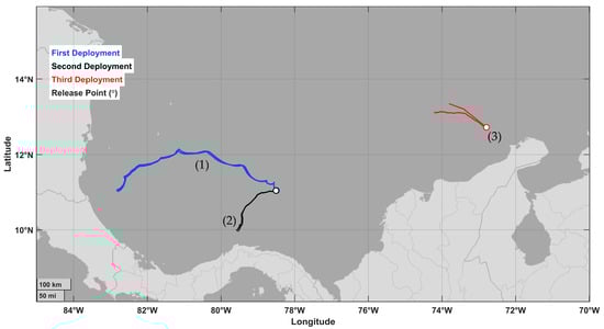
Figure 1.
Map of the Caribbean Sea showing the initial positions and trajectories of the released objects: (1) five drifters on 7 July 2024; (2) two drifters on 28 December 2024; (3) one mannequin (10 July 2025, 22:08 (UTC)) and two drifters (11 July 2025, 06:14 (UTC)).
2.2. Methodology
2.2.1. Direct and Inverse Problems
The telegraph equation is a widely recognized solution to diffusion problems, particularly those in which the propagation of a property must be constrained, a task that parabolic equations are unable to fulfill. In the case of a SAR operation, the property is defined as the initial probability field of an accident, denoted by P(x,y,t = T), within the horizontal space of the sea surface S, with coordinates x and y, and within the time interval of uncertainty T.
Therefore, the two-dimensional telegraph equation is hereby presented in the domain ⊂ {−∝ < x,y < +∝, 0 ≤ t ≤ T} as follows:
where a and W are constants that characterize the frequency of changes in the state of the diffusion process and the speed of turbulent pulsations, respectively.
Monin & Yaglom [7] mention that, in the case of a → ∞ and W → ∞, while their ratio remains finite, the hyperbolic Equation (1) reduces to a diffusion equation. The advantage of Equation (1) lies in the precise definition of the contour P = 0 in the searching field for objects at sea. It is evident that the first initial condition for (1) should be expressed as follows:
and the second is
with the value still undetermined.
According to the Second Law of Thermodynamics, the increase in the distance between the trajectories of drifters at sea should be inversely proportional to the probability of the field P. Thus, where P0 = 1 and λ represents the Lyapunov exponent. Thus, , so for t = 0 in (3),
Given the above result, Equation (1) can be rewritten as follows:
Here, δ(.) is the Dirac delta function, and is the coordinate vector with the point corresponding to the reported accident location at time t = 0. The second initial condition is now part of Equation (5), and the boundary conditions are as follows:
It is important to note, that since is a constant, .
Equation (5), along with conditions (2) and (6), is a well-posed direct problem. Let us formulate the inverse problem. To do so, we will introduce the scalar multiplication of two functions, a and b, in a Hilbert space, as follows:
Equation (5) is formally presented as
where and . The sameness of Lagrange
This leads to the conjugate equation to (8):
The above equation has operator , while expression (9) is a functional, whose dual representation is
The right-hand side defines the meaning of , assigning a specific expression to the function , while the left-hand side will be used to solve the optimization problem of the parameters a and W in (1), based on the theory of small perturbations.
It should be noted that the conjugate Equation (10) is solved in inverse time in the interval t ∈ [T,0] with the conditions
2.2.2. Parameter Optimization
The system parameters (a, W, must be re-evaluated at the onset of each SAR operation, based on observations from drifting buoys that can be deployed once the fleet reaches the approximate accident site. The uncertainty time is denoted as T, and the corresponding uncertainty area within this interval must be determined with the highest possible accuracy.
Deploying multiple drifters from the same location enables the estimation of the Lyapunov exponent . In such cases, or when only a single drifter is available, the parameters a and W can be adjusted accordingly.
Initial parameter values were obtained from a study conducted in the Caribbean Sea, where drifters were released at the coordinates specified in the following Chapter, and the Lagrangian timescale was computed from the autocorrelation of buoy velocity anomalies:
The timescale characterizes the memory of the process and is inversely related to parameter a: , where the constant must be determined. The parameter W is assumed to scale linearly with the r.m.s. of turbulent velocity fluctuations, , according to , where remains to be specified.
The parameter search was performed using a variational analysis over a physically consistent range of a and W, by minimizing the error function , where and denote the variances of current velocity oscillations obtained from the telegraph model and the buoy observations, respectively.
The optimization was performed over a temporal window of 6 h after each drifter release, corresponding to the Lagrangian decorrelation time Ti. Drifter velocity anomalies were first filtered using a second-order Butterworth low-pass filter with a cutoff of 1/Ti. The parameters a and W were co-estimated by minimizing the normalized variance misfit between modeled and observed velocity oscillations. The Lyapunov exponents were estimated following the standard procedure outlined in [17].
2.2.3. The Perturbation Theory
It should be remembered that with the right-hand side of the dual presentation (11) we define or assign the meaning of the functional J, while the left-hand side performs the calculation. The dimensions of the conjugate function P* are arbitrary and depend entirely on the choice of the handling or cost function g. The function f has clear quadratic frequency dimensions, and the units we are going to use are Hz2.
Considering that the definition of the functional
The handling function may be specified as
With the known fields P(x, y, t) from the direct problem (5), (2), and (6). In this and only this case, the functional J = (P, g) represents the rate at which the probability area increases within the interval [0, T]. The variation in the functional, δJ = F(δa, δW, ), helps to minimize the following invariant:
The unperturbed value of is calculated using the initial parameters a and W, which were previously calibrated using the above-described procedure; is the spatial variance given by buoys data, recollected hours after the accident.
Now, the theory of small perturbations is applied to the functional J,
Finally, we have
Our task is to find the optimal values of parameters
For each SAR operation, more than one drifter is available in the approximate search field. The procedure consists of solving the direct problem (5) with (2–4, 6), followed by the inverse problem (10), (12), and (13); then performing the optimization (18) using (15) and (17), and subsequently solving the direct problem again. As a result, the initial search area is obtained in a form like a Gaussian distribution, but with finite boundaries.
2.2.4. Lagrangian Model
Once the parameters (18) are adjusted by minimizing the functional (15), the initial search field is transformed into Lagrangian coordinates through the release of tracers, whose chaotic distribution corresponds to the probability value P(x,y,t = T). Tracer advection is performed using data from the Operational Mercator global ocean analysis and forecast system (sea-surface currents and sea-surface wave Stokes drift) [21] and a stochastic Lagrangian model, based on first-order autoregressive schemes, AR(1) [12]. Upon completion of the probabilistic forecast, the tracer cloud is converted into Eulerian fields P(x,y,t > T).
3. Results
3.1. Previous Experiments
On 7 July 2024, with the support of an oceanographic vessel of the Colombian Navy, five drifters were deployed at the position shown in Figure 1. The same procedure was subsequently repeated at another location. Based on these deployments, the Lyapunov exponents were calculated in order to run the direct model (2)–(6) multiple times, varying the parameters a and W over a range of real values. The buoy data were processed in such a way that the vector of currents was extracted, which in the model is defined by the combination of surface currents and Stokes drift obtained from the Copernicus platform [21]. The residual from this extraction corresponds to turbulent pulsations experienced by the drifters.
The process of varying the error functional was carried out using the drifter data, comparing the areas under the probabilistic curve P(x,y,T), and the minimum of this value was identified, as shown in Figure 2, thereby characterizing the fundamental values of a and W. Figure 3 presents the shape of the initial distribution of the search area for different values of the Lyapunov exponent.
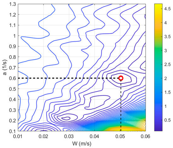
Figure 2.
Contours of as a function of parameters a and W, according to the methodology described in Section 2.2.2. The minimum of ε (red circle) is demonstrated for the parameters a = 0.6 s−1 and W = 0.05 m s−1.
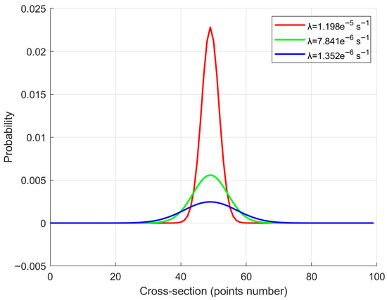
Figure 3.
Initial distribution of the search area [fields P(x,y,t = T)] and its sensitivity to the value of the Lyapunov exponent.
The identifiability of parameters a (state-change frequency) and W (propagation speed) was analyzed through a sensitivity study using synthetic perturbations of drifter velocities (±10%) and variations in the spatial variance field. The results showed that variations of ±10% in input drifter velocities lead to parameter variations of less than 7% in a and 9% in W, indicating acceptable robustness. Confidence intervals were found, showing ±0.04 s−1 for a and ±0.005 m s−1 for W. These ranges correspond to the minima of the error functional J(a, W) and represent the model’s intrinsic uncertainty in the Caribbean experiments.
Section 2.2.2 describes the methodology and refers to the constants C1 and C2, identified to relate the Lagrangian timescale Tᵢ, the pulsation velocity W, the frequency of state changes a, and the standard deviation of fluctuations σᵤ. The values obtained for these constants are C1 = 2318 and C2 = 1.22.
3.2. Data Assimilation
At 22:08 UTC on 10 July 2025, a man-overboard dummy equipped with satellite transmission was deployed in the Caribbean Sea. The deployment was carried out at coordinates 12.72° N, 72.79° W. The oceanographic vessel left the site and returned eight hours later to deploy, at the same location, two Stokes drifters manufactured by MetOcean Telematics, Canada. Based on this procedure, the search process for a floating object was simulated, representing the case of a person in the water.
- With the deployment of the two drifters, it was possible to conduct the complete procedure defined in Section 2.2.1, Section 2.2.3 and Section 2.2.4. The parameters a and W were adjusted using Equation (18), and the probabilistic search area was obtained, like that shown in Figure 3. From this area, the model was run, where the deterministic component consisted of the sum of surface current vectors and Stokes drift, provided by the Mercator operational forecasting system with hourly temporal discretization. Wind-induced leeway was not considered, as it is not relevant for a person in the water.
- Figure 4 shows the run of the AR(1) Lagrangian model and the deterministic component interpolated from the pseudo-hourly data at 10 min intervals. The transmissions from the dummy were intermittent; the timestamps of these transmissions are shown in Figure 4, numbered from 10 to 18, over a trajectory lasting 3.5 days. Consistency must be ensured between the time step (dt) of the Lagrangian model, the Lagrangian integral timescale (Ti), and the stochastic agitation prescribed within the AR(1) formulation. When dealing with a large ensemble of tracers (on the order of N = 106–109, depending on the oceanic scenario), the computational time becomes constrained by the need for a rapid model response. This leads to the practical dilemma of defining a time step dt that is sufficiently smaller than the memory scale Ti to preserve temporal coherence, yet large enough to maintain computational efficiency in SAR applications. In our simulations, a time step of dt = 0.1 Ti was adopted as a compromise between accuracy and speed, while the question regarding the optimal number of tracers N remains open and depends primarily on the available computational resources.
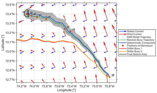 Figure 4. Trajectories of Lagrangian tracers (gray dots), their center of mass (blue line), and a particular tracer (green). Black dots show the trajectories of two drifting buoys released from the initial point (12.72° N, 72.79° W) eight hours after the release of the mannequin at hour 22:08 (UTC) (their reported positions are marked with red dots t0–t8). Red arrows represent the surface current field, while blue arrows denote the Stokes drift at the time of the mannequin release 10 July 2025, 22:08 (UTC) (Operational Mercator global ocean analysis and forecast system). The black contour represents the probability of the object’s final position, as shown in Figure 5.
 - Meanwhile, the drifters deployed hours later followed a different trajectory. However, the separation between the two drifters was minimal, only observable in the final segment shown in Figure 4.
- Figure 5 illustrates the field of the final probability distribution P(x,y) derived from the model versus the position of the dummy at the same instant.
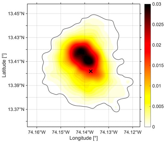 Figure 5. Final search field in terms of probability P(x,y) after 3.5 days of simulation. Point X indicates the mannequin position at the same time (corresponding to point t8 in Figure 4).
4. Discussion
First, it should be noted that, according to the results shown in Figure 5, the floating object was found within the probabilistic area despite 3.5 days of simulation and ocean current forecasting. Wind was not considered; however, its leeway factor can be readily integrated into the model according to the sail areas of each object in the case of vessels. These leeway factors are tabulated in the IAMSAR Manual [1]. An extensive report on the leeway factor for floating objects can be found in [9]. In that document, for persons in the water (PIW), this factor was evaluated for cases of a person sitting, or in a vertical or horizontal position, both with and without a diving tank. Our deployed dummy was in a vertical position, and based on the estimates summarized in [9], the wind-induced drift of a PIW in this position was determined to be approximately 0.5% of the wind speed. During the experiment, wind speeds ranged between 7 and 10 m/s, yielding a maximum drift velocity of less than 5 cm/s, which is much smaller than the effect of surface currents. However, this factor should be considered under other circumstances, where its influence may become significant.
The present study employs data assimilation at the level of parameter optimization rather than direct correction of the dynamic ocean fields. Specifically, drifter data are assimilated to update the stochastic parameters (a, W, λ) of the initial probabilistic field. In this context, the term ‘assimilation’ refers to the parameter-adjustment step that conditions the probabilistic field prior to Lagrangian advection. Conversely, if one were to assimilate the current data obtained from the drifters, Figure 4 demonstrates that this approach would fail: only eight hours after the incident, the released buoys exhibited a displacement direction completely different from that of the mannequin.
The probability field, when integrated over space, always yields a value of 1.0. The rescue strategy must therefore take into account this “zoning” obtained from the model. However, the field experiment results showed low divergence among the drifters deployed simultaneously. Essentially, Figure 4 demonstrates that the success of the operation depends almost entirely on the quality of the forecasts of surface ocean currents and Stokes drift. Two tracers corresponding to the center of mass of the particle clouds (propagation without diffusion) and any other tracer (Figure 4) indicate that their deviation is minimal, just as occurred with the drifters shown in the same figure. The drifters deployed hours later, however, exhibited markedly different trajectories due to changes in the hydrodynamic fields within only a few hours.
Figure 5 clearly illustrates the success of the experiment: the search object was located within the probabilistic field rather than outside it. However, to quantify this outcome, two diagnostic metrics were evaluated: (1) Containment probability, defined as the fraction of true drifter positions falling within the 95% iso-probability contour (value = 0.93); and (2) Brier Score, computed from the probabilistic field and observed positions, yielding BS = 0.067. Together, these metrics provide quantitative confirmation that the model’s probabilistic forecast achieves performance levels consistent with operational SAR applications.
To examine how the initial probability fields affect the forecast outcome as compared to a single initial search point, it was necessary to conduct an additional experiment with tracers released at different coordinates in the Caribbean Sea. Figure 6 presents the result of this simulation. From this figure it can be observed that, when accounting for the uncertainty of the initial position, the search area must be extended. Figure 6 shows the time history of the Lagrangian tracers as they follow the ocean currents. The width of the search area varies significantly, ranging from 1.3 nautical miles to 2.3 nautical miles (characteristic values) when applying the methodology developed in this paper.
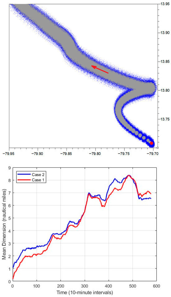
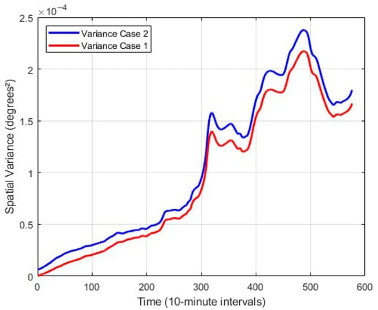
Figure 6.
(Top): Fragment of the trajectories of an object at sea, originating from a single point (red point, gray trajectory) and from a finite initial probabilistic area (blue trajectory). (Middle): Mean dimensions of the probabilistic areas along the respective trajectories. (Bottom): Spatial variance as a function of time. Case 1: single initial point; Case 2: finite initial area, computed using the proposed model.
The metrics in Figure 6 were calculated based on the distances between each tracer for every 10 min time interval, corresponding to a new probabilistic field. It can be observed that, although the finite initial area should generate a greater amplification of the field , there are time periods when the trajectories converge (negative values of the Lyapunov exponents), which is related to the hydrodynamic conditions and, likely, inertial oscillations. The first loop of these oscillations can be observed in Figure 6 in the vicinity of 13.8° N, 79.7° W.
Figure 6 shows significant differences between simulated Cases 1 and 2, where Case 1 corresponds to a single initial point of the incident, while Case 2 applies a finite initial area. The differences reach up to 1.0 nautical miles when the probabilistic field extends over 2.0 nautical miles, i.e., about 50%. Based on the variance values, the 3 r.-m.-s. value reaches 0.8 nautical miles.
5. Conclusions
The new method described in this work addressed the issue of uncertainties in the initial position of a maritime accident. At times, this position was not known with sufficient accuracy, and other factors related to hydrodynamics affected the probabilistic fields. Until now, SAR manuals had outlined the zoning of the search in an empirical manner, although they encouraged the application of numerical models to improve this process [1].
The Gaussian bell proposed by the IAMSAR Manual [1] corresponded to a normal distribution, whose nature is the solution of parabolic diffusion equations. A parabolic equation possesses an infinite propagation speed of the fields and therefore could not be used to define the initial search area; instead, a finite boundary of the probabilistic limit was required. Consequently, a hyperbolic telegraph-type equation, combining the properties of waves and diffusion, was able to define finite probability fields. This required determining the model parameters based on field experiments with drifting buoys, along with an adjustment of these parameters whenever the SAR process was carried out.
When the first part of the problem was solved through direct optimization of parameters, the second part assimilated the data and required the application of adjoint problems, the theory of small perturbations, and the use of ill-posed problems.
Figure 7 illustrates the flow of the process described here. Three options are shown, depending on the availability of drifting buoys in the SAR procedure: only with two or more drifters can the full information on the stochasticity of the processes be assimilated, allowing the three key parameters to be calibrated in detail; with a single drifting buoy, the Lyapunov exponent cannot be determined, and its value must be taken from historical data or obtained, for instance, from AVISO (aviso@info.altimetry.fr). Without the use of drifting buoys, the inverse problem does not apply, and the parameters cannot be adjusted.
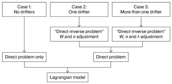
Figure 7.
Computation flowchart for the three cases of drifting buoy availability in the SAR process.
A combination of Eulerian and Lagrangian methods completed the task, demonstrating as a result that the search field, starting from an initial field, was about 50–60% larger compared with the case considering only a single initial accident point.
The SAR experiment was conducted under Caribbean Sea conditions. What could be the performance of the method under other oceanic conditions?
First of all, it should be noted that in the Caribbean, swell waves are almost never present, while sea waves are relatively short with high steepness values. This clearly affects the differences in Stokes drift and its role in the displacement of objects and PIWs. The relatively mild wind regime (despite the predominance of the trade winds in the Caribbean) differs from other oceanic regions; an increase in wind speed within frontal cyclonic systems enhances leeway drift.
In any case, this study makes it clear that the quality of the probabilistic forecast is directly correlated with the accuracy of wind, ocean current, and wave forecasts. However, the main goal of this work was to address the uncertainty of the initial search area, which is not considered in current models such as SAROPS and OpenDrift, whose use is typically based on estimating a single resultant displacement vector for the objects, rather than on non-stationary hydrodynamic fields. In a way, the present study contributes to the recommendations in manual [1] regarding the increased use of computational resources and methods in SAR operations.
Author Contributions
Conceptualization and methodology, S.L.; software, S.L. and J.N.; validation, S.L., I.P. and C.R.-B.; data curation, I.P. and C.R.-B.; writing—original draft preparation, S.L. and I.P.; writing—review and editing, S.L.; visualization, J.N.; supervision, C.R.-B.; project administration, C.R.-B.; funding acquisition, C.R.-B. All authors have read and agreed to the published version of the manuscript.
Funding
This research was conducted within the framework of Project 82863 “Optimization of the Search and Rescue (B&R) procedure at sea with naval operations”, with resources from the Ministry of Science, Technology, and Innovation, “Francisco Jose de Caldas” fund (1022-2020), within the framework of the “Call for Proposals for the implementation of R+D+I projects aimed at strengthening the ARC’s R+D+I portfolio, in accordance with its priorities and needs-2020”.
Data Availability Statement
The raw data supporting the conclusions of this article will be made available by the authors on request.
Acknowledgments
We are grateful to the Colombian Maritime Authority (DIMAR) and the crews of the oceanographic vessel ARC “Roncador” and the Colombian Navy Oceanic Patrol Vessel ARC “20 de Julio” for their support in the deployment of drifters and the manikin at sea. We also thank the Ministry of Science, Technology, and Innovation of Colombia; the Science and Technology Directorate of the Colombian Navy, especially to Rafael Hurtado Valdivieso, and Tecnalia Colombia for managing the research project.
Conflicts of Interest
The authors declare no conflicts of interest.
Abbreviations
The following abbreviations are used in this manuscript:
| SAR | Search And Rescue |
| IAMSAR | International Aeronautical and Maritime Search and Rescue |
| NSARC | National Search and Rescue Committee |
| PIW | Persons in Water |
| CASP | Computer-Assisted Search Program |
References
- International Maritime Organization & International Civil Aviation Organization. International Aeronautical and Maritime Search and Rescue Manual. Volume 1. Organization and Management; International Maritime Organization: London, UK, 2022; 164p. [Google Scholar]
- National Search and Rescue Committee [NSARC]. National Search and Rescue Supplement to the International Aeronautical and Maritime Search and Rescue Manual (NSS); United States Government Printing Office: Washington, DC, USA, 2013.
- Cooper, D.; Frost, J.; Robe, R. Compatibility of Land SAR Procedures with Search Theory; Department of Homeland Security, United States Coast Guard, Operations (G-OPR): Washington, DC, USA, 2003. [Google Scholar]
- Kilic, K.; Maity, S.; Sung, I.; Nielsen, P. Challenges and AI driven solutions in maritime search and rescue. Mar. Policy 2025, 178, 106692. [Google Scholar] [CrossRef]
- Fontanelli, O.; Mansilla, R.; Miramontes, P. Distribuciones de probabilidad en las ciencias de la complejidad: Una perspectiva contemporánea. Scielo 2020, 8, 11–37. [Google Scholar] [CrossRef]
- International Maritime Organization & International Civil Aviation Organization. International Aeronautical and Maritime Search and Rescue Manual. Volume 2. Mission Coordination; International Maritime Organization: London, UK, 2022; 548p. [Google Scholar]
- Breivik, O.; Allen, A. An operational search and rescue model for the Norwegian Sea and North Sea. Mar. Syst. 2008, 69, 99–113. [Google Scholar] [CrossRef]
- Richardson, H.; Discenza, J. The United States Coast Guard Computer Assisted Search Planning system (CASP). Nav. Res. Logist. Q. 1980, 27, 659–680. [Google Scholar] [CrossRef]
- Allen, A.; Plourde, J. Review of Leeway: Field Experiments and Implementation; Final Report, Report No. CG-D-08-99; United States Coast Guard, U.S. Department of Transportation: Washington, DC, USA, 1999.
- Breivik, O.; Allen, A.; Maissondieu, C. Wind-induced drift of object at sea: The leeeway field method. Appl. Ocean Res. 2011, 33, 100–109. [Google Scholar] [CrossRef]
- Spaulding, M.; Isaji, T.; Hall, P.; Allen, A. A Hierarchy of Stochastic Particle Models for Search and Rescue (SAR): Application to Predict Surface Drifter Trajectories Using HF Radar Current Forcing. J. Mar. Environ. Eng. 2006, 8, 181–214. [Google Scholar]
- Griffa, A. Applications of stochastic particle models to oceanographic problems. In Stochastic Modelling in Physical Oceanography; Birkhäuser: Boston, MA, USA, 1996; pp. 113–128. [Google Scholar]
- Berloff, P.; McWilliams, J. Material transport in oceanic gyres. Part II: Hierarchy of stochastic models. J. Phys. Oceanogr. 2002, 32, 797–830. [Google Scholar] [CrossRef]
- Bezgodov, A.; Dmitrii, E. Complex Network Modeling for Maritime Search and Rescue Operations. Procedia Comput. Sci. 2014, 29, 2325–2335. [Google Scholar] [CrossRef][Green Version]
- Romero-Balcucho, C. Stochastic Dynamic Model for Search and Rescue Operations at Sea. Master’s Thesis, Master’s Degree Colombian Navy Academy, Cartagena, Colombia, 11 October 2015. [Google Scholar]
- Marchuk, G.I.; Kagan, B.A. Theory of Tides: Ocean Tides. Mathematical Models and Numerical Experiments; Pergamon Press: New York, NY, USA, 1984; 292p. [Google Scholar]
- Monin, A.; Yaglom, A. Statistical Fluid Mechanics: The Mechanics of Turbulence; The Massachusetts Institute of Technology: Cambridge, MA, USA, 1973; Volume 1, 782p. [Google Scholar]
- Okubo, A. Application of the Telegraph Equation to Oceanic Diffusion: Another Mathematical Model; Chesapeake Bay Institute, The Johns Hopkins University: Baltimore, MD, USA, 1971; 43p. [Google Scholar]
- Westerterp, K.; Dil’man, V.; Kronberg, A. Wave model for longitudinal dispersion: Development of the model. AIChE J. 1995, 41, 2013–2028. [Google Scholar] [CrossRef]
- Boudreau, B. A theoretical investigation of the organic carbon–microbial biomass relation in muddy sediments. Aquat. Microb. Ecol. 1999, 17, 181–189. [Google Scholar] [CrossRef]
- European Union-Copernicus Marine Service. Global Ocean 1/12° Physics Analysis and Forecast Updated Daily [Dataset]. Mercator Ocean International. Available online: https://data.marine.copernicus.eu/product/GLOBAL_ANALYSISFORECAST_PHY_001_024/description (accessed on 10 July 2024).


Disclaimer/Publisher’s Note: The statements, opinions and data contained in all publications are solely those of the individual author(s) and contributor(s) and not of MDPI and/or the editor(s). MDPI and/or the editor(s) disclaim responsibility for any injury to people or property resulting from any ideas, methods, instructions or products referred to in the content. |
© 2025 by the authors. Licensee MDPI, Basel, Switzerland. This article is an open access article distributed under the terms and conditions of the Creative Commons Attribution (CC BY) license (https://creativecommons.org/licenses/by/4.0/).